

1. Introduction
The instability of the flow in a channel with wavy walls is used as a model for flow instabilities caused by wall roughness. Vortex–wave interaction theory has previously been used to describe nonlinear exact coherent structures but here we uncover a mechanism by which wall roughness enables the typical roll–streak–wave interaction to occur in the linear regime. We stress that we are not discussing the role of roughness in the receptivity process for classical instabilities such as Tollmien–Schlichting waves, see for example Ruban (Reference Ruban1983) or Goldstein (Reference Goldstein1983), but what is best described as a parametric instability relevant to quite arbitrary shear flows over rough walls. It is well known that curved walls lead to centrifugal instabilities in the form of Taylor or Görtler vortices; see for example Hall (Reference Hall1983). However, the instability described here is not of the centrifugal type because the coupling between rolls and streaks which constitute such instabilities is not through centrifugal effects but by a rather subtle interaction close to the wall involving waves, rolls and the local topography.
Interest in heat transfer mixing devices in laminar flow configurations provides part of the motivation for the present study. The reader is referred to, for example, Bergles & Webb (Reference Bergles and Webb1985) and Ligrani, Oliveira & Blaskovich (Reference Ligrani, Oliveira and Blaskovich2003) for a discussion of the effect on heat transfer of modifications to channel geometry. Experimental evidence for the existence of streamwise vortex instabilities in sinusoidal channels is given by Gschwind, Regele & Kottke (Reference Gschwind, Regele and Kottke1995) and Nishimura, Yoshino & Kawamura (Reference Nishimura, Yoshino and Kawamura1987). Related instabilities in pipes of periodically varying radius have been found in Navier–Stokes simulations by Loh & Blackburn (Reference Loh and Blackburn2011). On the theoretical side the papers most relevant to the present study are those of Floryan (Reference Floryan2003, Reference Floryan2015) on pressure gradient driven flows and Floryan (Reference Floryan2002) on Couette flow. In Floryan (Reference Floryan2003) a channel with walls having undulations of the same amplitude  $\epsilon$ but half a wavelength out of phase was considered. In Floryan (Reference Floryan2015) walls with undulations in phase were considered. Results were given for quite small amplitude undulations and, though no discussion of this point is given in Floryan (Reference Floryan2015), the corresponding results in Floryan (Reference Floryan2003, Reference Floryan2015) appear to be indistinguishable. Floryan (Reference Floryan2002) proposed a curve fit which has the critical Reynolds number scaling like
 $\epsilon ^{-1.29}$, and based on a comparison of the relevant figures in Floryan (Reference Floryan2003, Reference Floryan2015) work that curve fit applies equally well to both papers.
Here, we will derive an asymptotic form for the critical Reynolds number in terms of  $\epsilon$, unlike the curve fit the asymptotic solution involves powers of both
 $\epsilon$ and
 $\vert {\log \epsilon }\vert$. We will explain the similarity of the results in Floryan (Reference Floryan2003, Reference Floryan2015). In spite of the complexity of the interaction driving the instability, it turns out that we can solve the leading-order problem analytically and write down an expression for the neutral configuration. The results agree with the full numerical solutions of the above papers on Poiseuille and Couette flow and the interaction derived applies to quite arbitrary internal and external shear flows over rough walls. In the next section we will derive the asymptotic description of the instability and then in § 3 apply the results to Poiseuille and Couette flow. In § 4 we will draw some conclusions.
2. The base flow and stability problem
Consider the viscous incompressible flow in the channel  $[-1+\epsilon F(x)] \le y \le [1+\epsilon G(x)].$ Here
 $F,G$ are periodic in
 $x$ but not necessarily of the same wavelength or amplitude. The parameter
 $\epsilon$ is small and the flow is driven by a combination of a streamwise pressure gradient and the motion of the upper wall in the
 $x$ direction. If the wall undulations are to be thought of as a model of wall roughness then
 $F,G$ would also be dependent on
 $z$. That is beyond the scope of the present investigation but we believe the approach could be extended to cover that case. We write the equations of motion in the dimensionless form
 \begin{equation} \frac{\textrm{D} {{\boldsymbol{{u}}}}}{\textrm{D} t} = {-\boldsymbol{\nabla}}p + \frac{1}{R}\nabla^{2}{{\boldsymbol{u}}},\quad \boldsymbol{\nabla} \boldsymbol{\cdot} \boldsymbol{u} = 0. \end{equation}
Here u and p are the fluid pressure and density, and  $R$ is the Reynolds number and in the absence of wall undulations the basic state is a unidirectional flow in the
 $x$ direction given by
 \[ {\boldsymbol{{u}}}={\boldsymbol{{u_b}}} =(u_0 (\,y), 0,0)=([1-y^2]+U^+y, 0, 0),\quad p=p_0(x)= -\frac{2x}{R}, \]
with  $U^+$ the scaled speed of the upper wall. Suppose the above flow, with
 $\epsilon =0$, is perturbed by a small streamwise vortex disturbance of size
 ${\rm \Delta}$, spanwise wavenumber
 $k$ and growth rate
 $\sigma$ by writing
 \begin{gather*} {\boldsymbol{{u}}} ={\boldsymbol{{u_b}}}+{\rm \Delta} \left(U_0(y)\cos kz, \frac{1}{R} V_0(y)\cos kz, \frac{1}{R} W_0(y)\sin kz\right)\textrm{e}^{{\sigma t}/{R}},\\ p = p_0(x)+ \frac{{\rm \Delta} }{ R^2}P(y)\,\textrm{e}^{{\sigma t}/{R}}\cos kz. \end{gather*}
Linearising the equations of motion it is easy to show that
 \begin{gather} \left[\frac{\textrm{d}^2}{\textrm{d} y^2}- k^2 - \sigma\right]U_0 = V_0 u_0',\quad \left[\frac{\textrm{d}^2}{\textrm{d} y^2}- k^2 - \sigma\right]V_0 = \frac{\textrm{d} P_0}{\textrm{d} y}, \end{gather}
 \begin{gather}\left[\frac{\textrm{d}^2}{\textrm{d} y^2}- k^2 - \sigma\right]W_0 = -k P_0,\quad \frac{\textrm{d} V_0}{\textrm{d} y} +kW_0 =0. \end{gather}
If the walls are flat then the above equations are solved subject to no slip at  $y= \pm 1$ and we obtain two sets of stable eigenvalues. The first set corresponds to setting
 $U_0=0$ and the second set has
 $V_0=W_0=0.$ In a curved channel the equations couple through a centrifugal term proportional to
 $u_0 U_0$ in the
 $y$ momentum equation and instability is possible. We will show how the usual no-slip conditions appropriate to (2.2)–(2.3) are modified by undulations of size
 $\epsilon$ at high Reynolds numbers. The analysis is motivated by Hall & Smith (Reference Hall and Smith1991) and Hall & Sherwin (Reference Hall and Sherwin2010) who considered vortex–wave interactions in shear flows. In those papers a closed system of equations coupling rolls, streaks and waves in shear flows was derived asymptotically and used to describe with remarkable accuracy Navier–Stokes calculations of exact coherent structures. In the latter papers the crucial step was to find the asymptotic scaling for a wave system existing as a neutral mode of the streak flow able to drive the roll flow which itself drives the streak. Here, the roll–streak flow corresponds to
 ${\boldsymbol {u_0}+\boldsymbol {U_0}}$ but now
 $\boldsymbol {U_0}$ is too small to allow unstable inviscid waves and the tripartite coupling is facilitated by the wall. At this stage we assume that
 $\epsilon$ is small compared to
 $R^{-({1}/{3})}$, note that
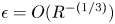 $\epsilon = O( R^{-({1}/{3})})$ is the interactive regime where the wall amplitude is comparable with the viscous boundary layer at the wall; see Smith (1982). The key point is that roll–streak flows have the roll velocities smaller by a factor of
 $R^{-1}$ than the streak so that small waves big enough to interfere with the roll thus have an
 $O(1)$ effect on the streak.
We assume the wall undulations are periodic in  $x$ and, apart from having amplitudes of the same order of magnitude as
 $\epsilon$, can be quite general. Suppose that
 $F = 2 \cos \alpha _1 x, G=2 \Gamma \cos \alpha _2 x$ with independent wavenumbers
 $\alpha _1, \alpha _2$. Thus
 $\Gamma$ is the relative size of the wall undulations. We initially assume
 $R=O(1)$ and for the moment take
 $\alpha _1=\alpha _2$ and modify the perturbed base flow to account for the presence of the wall undulations by writing
 \begin{gather} u= u_0(y) +\epsilon (u_1(y)E+{\rm c}.{\rm c}.) +\cdots +{\rm \Delta} [U_0(y)+\epsilon (U_1(y)E+{\rm c}.{\rm c}.)+\cdots]\,\textrm{e}^{{\sigma t}/{R}}\cos kz \end{gather}
 \begin{gather}v= 0+\epsilon (v_1(y)E+{\rm c}.{\rm c}.) +\cdots + {{\rm \Delta} } \left[\frac{V_0(y)}{R}+\epsilon (V_1(y)E+{\rm c}.{\rm c}.)+\cdots\right] \textrm{e}^{{\sigma t}/{R}}\cos kz \end{gather}
 \begin{gather}w= 0 + {{\rm \Delta}} \left[\frac{W_0(y)}{R}+\epsilon (W_1(y)E+{\rm c}.{\rm c}.)+\cdots\right]\textrm{e}^{{\sigma t}/{R}}\sin kz \end{gather}
 \begin{align} p &= p_0(x)+ \epsilon (p_1(y)E+{\rm c}.{\rm c}.) +\cdots)+ {{\rm \Delta} } \left[\frac{P_0(y)}{R^2}+\epsilon (P_1(y)E+{\rm c}.{\rm c}.)+\cdots\right] \nonumber\\ &\quad \times\textrm{e}^{{\sigma t}/{R} } \cos kz, \end{align}
where  $E=\textrm {e}^{\textrm {i} \alpha _1 x}$ and
 $\ldots$ denotes terms of smaller size in
 $\epsilon$. Substituting the above into the equations of motion and comparing terms of size
 $\epsilon$, eliminating
 $v_1, p_1$ it is easy to show that
 $v_1$ satisfies the Orr–Sommerfeld equation
 \[ u_0\left(\frac{\textrm{d}^2}{\textrm{d} y^2}-\alpha_1^2\right)v_1-u''_0v_1= \frac{1}{\textrm{i} \alpha_1 R} \left(\frac{\textrm{d}^2}{\textrm{d} y^2}-\alpha_1^2\right)^2v_1, \]
and the no-slip condition is satisfied at the lower wall if
 \[ v_1 (-1)=0,\quad v'_1 (-1)= \textrm{i}\alpha_1 \lambda_1. \]
Here,  $\lambda _1 = u_0'(-1)$, assumed without loss of generality to be positive, is the unperturbed wall shear at the lower boundary. For large
 $R$ the right-hand side of the equation for
 $v_1$ can be ignored but near
 $y=-1$ there is a viscous layer of thickness
 $R^{-({1}/{3})}$ and in terms of
 $\xi =( \textrm {i} \lambda _1 R)^{{1}/{3}}[1+y]$ the leading-order problem near the lower wall is
 \[ \frac{\textrm{d}^4 v_1}{\textrm{d} \xi^4}-\xi \frac{\textrm{d}^2 v_1}{\textrm{d} \xi^2}=0,\quad v_1=0,\quad v'_1= (\textrm{i} \alpha_1 \lambda_1)^{{2}/{3}} R^{-({1}/{3})},\quad \xi=0, \]
so that  $v_1= 3(\textrm {i} \alpha _1 \lambda _1)^{{2}/{3}} R^{-({1}/{3})}\int ^\xi _0 \textrm {d} \eta \int ^\infty _\eta \textrm {Ai}(\theta )\,\textrm {d}\theta ,$ where Ai is the Airy function and we deduce that
 \begin{equation} v_1 \rightarrow \frac{\textrm{i}^{{2}/{3}}}{{R}^{{1}/{3}}}v_{\infty},\quad v_{\infty}=-3 \textrm{Ai}'(0)(\alpha_1 \lambda_1)^{{2}/{3}},\quad \xi \rightarrow \infty. \end{equation}
Note that  $u_1$ is
 $O(1)$ in the wall layer but falls to
 $O(R^{-({1}/{3})})$ at the edge of the layer. This means that for
 $y=O(1)$
 $u_1,v_1$ in (2.4)–(2.5) are both
 $O(R^{-({1}/{3})})$. A similar analysis is possible for
 $U_1, V_1, W_1, P_1$ which is driven by the need for
 $U_0$ to vanish at the lower wavy wall. An analysis accounting for the
 $z$ variation gives
 \begin{equation} V_1 \rightarrow \frac{2 \,\textrm{i}^{{2}/{3}}}{3{R}^{{1}/{3}}} \frac{U_0'(-1) }{ \lambda_1 }v_{\infty},\quad \xi \rightarrow \infty. \end{equation}
Note that the extra factor of  $\frac {2}{3}$ appearing above arises because of the extra terms which force the equation for
 $V_1$ in the viscous layer. In the core region the three velocity components needed to match onto the above limiting forms must be of the same size because variations in the
 $x,y,z$ directions are on the same scale. Thus, in the high Reynolds number limit in the core region, the finite
 $R$ expansions (2.4)–(2.7) must be replaced by
 \begin{align} u &= u_0(y) +\epsilon R^{-({1}/{3})} (u_1(y)+{\rm c}.{\rm c}.) +\cdots \nonumber\\ &\quad +{\rm \Delta}[U_0(y)+\epsilon R^{-({1}/{3})} (U_1(y) {E}+{\rm c}.{\rm c}.)+\cdots]\,\textrm{e}^{{\sigma t}/{R} }\cos kz \end{align}
 \begin{align} v &= 0+\epsilon R^{-({1}/{3})} (v_1(y) {E}+{\rm c}.{\rm c}.) +\cdots \nonumber\\ &\quad + {\rm \Delta}\left[\frac{V_0(y)}{R}+\epsilon R^{-({1}/{3})}(V_1(y) {E}+{\rm c}.{\rm c}.)+\cdots\right]\textrm{e}^{{\sigma t}/{R} }\cos kz \end{align}
 \begin{align} w &= 0 + {{\rm \Delta} } \left[\frac{W_0(y)}{R}+\epsilon R^{-({1}/{3})}(W_1(y) {E}+{\rm c}.{\rm c}.)+\cdots\right]\textrm{e}^{{\sigma t}/{R} }\sin kz \end{align}
 \begin{align} p &= p_0(x)+ \epsilon R^{-({1}/{3})} ((p_1(y) {E}+{\rm c}.{\rm c}.) +\cdots) \nonumber\\ &\quad + {{\rm \Delta} }\left[\frac{P_0(y)}{R^2}+\epsilon R^{-({1}/{3})}(P_1(y) {E}+{\rm c}.{\rm c}.)+\cdots\right]\textrm{e}^{{\sigma t}/{R} } \cos kz. \end{align}
Note at this stage we are still to fix the size of  $\epsilon$ compared to
 $R$ but we have implicitly assumed above that
 $\epsilon \ll R^{-({1}/{3})}$. Substituting the above into the equations of motion and equating terms proportional to
 $\epsilon R^{-({1}/{3})}$ we find that
 $v_1$ satisfies
 \begin{equation} u_0\left(\frac{\textrm{d}^2}{\textrm{d} y^2}-\alpha_1^2\right)v_1-u''_0v_1=0,\quad v_1(-1)=\textrm{i}^{{2}/{3}}v_\infty. \end{equation}
At this stage the upper boundary condition remains unknown until the viscous layer is studied there, however, if the upper wall is flat the condition becomes simply  $v_1=0$ there. Note also that, even though (2.14) is singular at
 $y=-1$, the solution remains regular there. The leading-order approximation to the streamwise vortex terms independent of
 $x$ again yields (2.2)–(2.3) but we delay writing down the boundary conditions until later. If we now consider the leading-order streamwise vortex terms dependent on
 $x$ we obtain the inviscid system
 \begin{gather} \textrm{i} \alpha_1(U_0 u_1 +u_0 U_1)+V_1u'_0 +v_1 U'_0= -\textrm{i} \alpha_1 P_1, \end{gather}
 \begin{gather}\textrm{i} \alpha_1(U_0 v_1 +u_0 V_1) = - P'_1, \end{gather}
 \begin{gather}\textrm{i} \alpha_1 u_0 W_1 =kP_1, \end{gather}
 \begin{gather}\textrm{i} \alpha_1 U_1+V'_1-kW_1=0. \end{gather}
From the above equations we deduce that
 \begin{equation} u_0({V''_1-[\alpha_1^2+k^2]V_1)}-u''_0 V_1=-U_0(v''_1-[\alpha_1^2+k^2]v_1 )+U''_0 v_1, \end{equation}
so  $V_1$ satisfies the Rayleigh equation for an inviscid three-dimensional mode forced by a Rayleigh equation involving the known functions
 $v_1, U_0$; once again, a solution regular at
 $y=-1$ exists. The lower boundary condition on
 $V_1$ follows from (2.9).
The crucial step now is to provide closure of the systems for  ${\boldsymbol {U_0}, \boldsymbol {U_1}}$ because, as it stands, the system for
 ${\boldsymbol {U_0}}$ does not depend on the
 $x$-dependent streamwise vortex field
 ${\boldsymbol { U_1}}$. Next, we use what is essentially the vortex–wave interaction theory of Hall & Smith (Reference Hall and Smith1991) for Tollmien–Schlichting waves to achieve a coupling. We will see below that it is the behaviour of
 $W_1$ as the wall is approached which leads to the required closure. That behaviour is found by first using (2.15), (2.17), (2.18) to show that
 \[ (\alpha_1^2+k^2)P_1=\textrm{i} \alpha_1[V_1u_0'+v_1U_0'-U_0v_1'-u_0V_1']. \]
Thus, using (2.8), (2.9), we find that as the boundary is approached
 \[ (\alpha_1^2+k^2)P_1 \rightarrow \tfrac{5}{3}\textrm{i}^{{5}/{3}}\alpha_1v_{\infty}U_0'(-1), \]
and using (2.17) we deduce that
 \begin{equation} W_1 \simeq \dfrac{5 k{\rm i}^{{2}/{3}} v_{\infty} U'_0(-1)}{3 \lambda_1 [\alpha_1^2+k^2][y+1]},\quad y \rightarrow -1. \end{equation}
We now find the mean in  $x$ of the nonlinear terms in the spanwise momentum equation, that mean will depend on
 $z$. The key is to find that size of
 $\epsilon$ as it is increased when the forcing drives
 $W_0$ and thus provides closure. We first note from continuity that if
 $u,v,w$ are periodic in
 $x$ with wavelength
 ${2 {\rm \pi} }/{\alpha _1}$ then
 \[ \int_0^{{2 {\rm \pi}}/{\alpha_1}} (uw_x+v w_y+ww_ z )\,\textrm{d}\kern0.5pt x= \int_0^{{2 {\rm \pi}}/{\alpha_1}} ( [v w]_y+2w w _z)\,\textrm{d}\kern0.5pt x. \]
The first term in the integrand on the right-hand side above is  $O({\rm \Delta} )$ and so the second term which is
 $O(\Delta ^2)$ can be neglected. The dominant contribution then comes from the terms proportional to
 $v_1, W_1$ in (2.11), (2.12), respectively, and, using the already derived behaviour of those functions as the boundary is approached, we deduce that
 \[ \frac{\alpha_1}{2 {\rm \pi}}\int_0^{{2 {\rm \pi}}/{\alpha_1}} (uw_x+v w_y+ ww_ z)\,\textrm{d}\kern0.5pt x \simeq -\frac{10 {\rm \Delta} \epsilon^2 { k v^2_{\infty} U'_0(-1)} }{3 R^{{2}/{3}} \lambda_1 [\alpha_1^2+k^2] [y+1]^2} \sin kz,\quad y \rightarrow -1. \]
This singular behaviour of the nonlinear terms in the spanwise momentum equation is similar to the vortex–TS/wave interaction problem of Hall & Smith (Reference Hall and Smith1991) and means that within the  $z$ momentum equation the nonlinear terms will drive a roll flow. That
 $x$-independent flow in the
 $y-z$ plane is of size
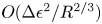 $O({{\rm \Delta} \epsilon ^2}/{R^{{2}/{3}}})$ so, if we take the
 $z$ velocity component of the induced roll flow to be
 ${\mathcal {W}}/{R}$, it follows that
 \[ \frac{\partial^2 {\mathcal{W}}}{\partial y^2}=-\frac{10{\rm \Delta} \epsilon^2 R^{{4}/{3}}k { v^2_{\infty} U'_0(-1)} } {3\lambda_1 [\alpha_1^2+k^2] [y+1]^2} \sin kz+\cdots, \]
as  $y \rightarrow -1$ so that the induced spanwise velocity has a logarithmic dependence as the wall approached.
The presence of the second derivative on the left-hand side and the factor  $(y+1)^{-2}$ on the right-hand side means that these terms remain in balance, however small we take
 $y+1$. That means that this same balance is maintained in the outer part of the viscous wall layer. In other words if we write
 $\zeta =(\lambda _1 \alpha _1 R)^{{1}/{3}} (1+y)$ and consider the form of the equation for
 $\mathcal {W}$ in the viscous wall layer then for large
 $\zeta$ it will take the same form as the above equation with
 ${\partial }/{\partial y}, y+1$ in that equation replaced by
 ${\partial }/{\partial \zeta }, \zeta$, respectively. Thus, on exiting the wall layer
 $\mathcal {W}$ will behave like
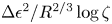 ${{\rm \Delta} \epsilon ^2}/{R^{{2}/{3}}} \log \zeta$. Now writing
 $\log \zeta = \log (1+y) +\frac {1}{3}\log (\lambda _1 \alpha _1 R)$ we deduce that the induced spanwise velocity field in the core will be of size
 ${{\rm \Delta} \epsilon ^2}/{R^{{2}/{3}}} \log (R)$ and driven by the interaction in the wall layer. Furthermore, the forcing in the core will then be negligible at leading order. We now close the problem by making the induced spanwise velocity in the core the same size as that of the assumed roll flow corresponding to
 $(V_0, W_0)$. Thus writing
 \[ \frac{\epsilon^2 \log(\lambda_1 \alpha_1 R)} {R^{{2}/{3}}}=\frac{R^*}{R^{2}} \]
means that the roll flow induced by the Reynolds stress terms in the wall layer will produce a roll flow of the same size as that assumed in (2.10)–(2.13) and we find that  $W_0$ in (2.12) must satisfy
 \begin{equation} W_0(-1)= \frac{10k R^* v^2_{\infty} U'_0(-1) }{9 \lambda_1 [\alpha_1^2+k^2]} +\cdots= \frac{10k \alpha_1^{{4}/{3}} \lambda_1^{{1}/{3}}R^* \textrm{Ai}' (0)^2 U'_0(-1) }{ [\alpha_1^2+k^2]}+\cdots, \end{equation}
and the forcing of the  $W_0$ equation is confined to the wall layer. Equation (2.21) thus connects the spanwise and streamwise velocity components of the imposed streamwise vortex
 $(U_0, V_0, W_0)$.
In Hall & Smith (Reference Hall and Smith1991) the forcing terms in the normal and streamwise momentum equations are negligible compared to that in the  $z$ direction, that is exactly the same here and so
 $U_0, V_0$ vanish at
 $y=-1$. In vortex–wave interaction theory the roll flow is sustained by a wave interacting with itself to drive the part of the flow independent of
 $x$ and the closure there is fixed by making the roll driven by that self-interaction to be comparable in size to the roll flow associated with the streak. Here, the interaction is driven by the
 $x$-dependent corrections to the unperturbed mean flow and the streamwise vortex
 $U_0$.
The analysis above can be repeated for the upper wall. If  $\alpha _1=\alpha _2$ we retain (2.10)–(2.13) without change, otherwise we need to add terms proportional to
 $\textrm {e}^{\pm \textrm {i}\, \alpha _2 x}$ of exactly the same form as those proportional to
 $\textrm {e}^{\pm \textrm {i}\,\alpha _1x}$. The analysis then goes through in exactly the same way in either case and leads to
 \begin{equation} W_0( 1)= \frac{10k \Gamma^2 \alpha_2^{{4}/{3}} \lambda_2^{{1}/{3}}R^* \textrm{Ai}' (0)^2 U'_0(-1) }{ [\alpha_2^2+k^2]}, \end{equation}
where  $\lambda _2$ is the modulus of the shear at the upper wall. From (2.21)–(2.22) we can immediately see that the relative phases of the undulations on the upper and lower walls plays no role in the interaction problem, that explains why the results of Floryan (Reference Floryan2003, Reference Floryan2015) should be identical. The functions
 $U_0, V_0$ vanish at the upper wall and so, eliminating the
 $P_0, W_0$ from (2.2)–(2.3), we have the eigenvalue problem
 \begin{gather} \left[\frac{\textrm{d}^2}{\textrm{d} y^2}- k^2 - {\sigma }\right]U_0 = V_0 u_0', \end{gather}
 \begin{gather}\left[\frac{\textrm{d}^2}{\textrm{d} y^2}- k^2 - {\sigma }\right] \left[\frac{\textrm{d}^2}{\textrm{d} y^2}- k^2 \right]V_0 = 0, \end{gather}
 \begin{gather}U_0=V_0=0,\quad y=\pm1, \end{gather}
 \begin{gather}k^{-1} V'_0(-1) = - \frac{10k \alpha_1^{{4}/{3}} \lambda_1^{{1}/{3}}R^* \textrm{Ai}' (0)^2 U'_0(-1) }{ [\alpha_1^2+k^2]}, \end{gather}
 \begin{gather}k^{-1} V'_0( 1)= - \frac{10k \Gamma^2 \alpha_2^{{4}/{3}} \lambda_2^{{1}/{3}}R^* \textrm{Ai}' (0)^2 U'_0( 1) }{ [\alpha_2^2+k^2]}. \end{gather}
The instability is the result of the interaction between surface undulations corresponding to  ${\boldsymbol {u_1}}$, a spanwise modulated wave corresponding to
 ${\boldsymbol {U_1}}$ and a streamwise vortex
 ${\boldsymbol {U_0}}$, yet this rather complex interaction reduces to the above simple eigenvalue problem. Indeed, we can solve the eigenvalue problem in closed form by first solving (2.24) subject to the required conditions on
 $V_0, V'_0$ and then solving (2.23) subject to
 $U_o(\pm 1)=0$. The solution will be a linear combination of terms proportional to
 $U'_0(\pm 1)$ and differentiating the solution and setting
 $y=\pm 1$ produces a pair of linear equations for
 $U'_0(\pm 1 )$ and, if we consider the neutral case with
 $\sigma =0$, the consistency of the equations produces a quadratic equation for
 $R^*$ so there will be two possible modes. If one wall is flat then either of the right-hand sides of (2.26), (2.27) vanishes and there is one mode of instability. Now let us examine the above prediction for some particular problems, the more general problem is solved as just indicated. The above discussion shows conclusively that in the high Reynolds number and small amplitude limit the walls act independently and there is no need to have the upper or lower walls of the same amplitude or wavelength or phase. The reason for this is that the mechanism driving the instability is the vortex–wave interaction at the edge of the viscous layers at the walls, and the crucial properties of that interaction are defined by the local geometry.
3. Results for Poiseuille and Couette flow
Let us now examine the two obvious prototype problems for the channel flow considered above. In the first case we consider Couette flow above a wavy wall and then consider Poiseuille flow with both walls having the same wavelength and amplitude.
3.1. Couette flow
We now suppose the flow under consideration is Couette flow over a small amplitude wavy wall so that  $u_0=y$. The growth rate of the vortex–wave instability considered in the previous section is determined by the eigenvalue problem (2.23)–(2.27) but with
 $\Gamma =0$ so that
 $V'_0(1)=0$. We consider the neutral case and, assuming the exchange of instabilities we set
 $\sigma =0$, solve for
 $V_0$ and then solve for
 $U_0$ vanishing at the boundaries. This gives a result of the form
 $U_0=U'_0(-1)q(y)$ where
 $q$ is a rather lengthy expression, for consistency we require
 $q'(-1)=1$, which after some algebra yields
 \begin{equation} R^*=\frac{2(\alpha^2_1+k^2)(\sinh^2 2k -4k^2)}{5 \alpha_1^{{4}/{3}} \textrm{Ai}' (0)^2 [\sinh^2 2k -8k^3 {\coth 2k }{ } ]}, \end{equation}
and then
 \begin{equation} R\simeq\frac{[2R^*]^{{3}/{4}}}{\epsilon^{{3}/{2}} [3 \vert{\log \epsilon}\vert]^{{3}/{4}}}. \end{equation}
Surprisingly, the instability which takes the form of a streamwise vortex interacting with a spanwise modulated wave and the topography has its neutral curve determined analytically. It follows immediately from (3.1) that  $R^* \simeq k^{-2}, k^2$ for small and large
 $k$ with
 $\alpha _1$ fixed and
 $R^* \simeq \alpha _1^{ -{({4}/{3})}}, \alpha _1^{{2}/{3}}$ for small and large
 $\alpha _1$ with
 $k$ fixed. Thus, there will be instability for all values of
 $\alpha _1, k$ if
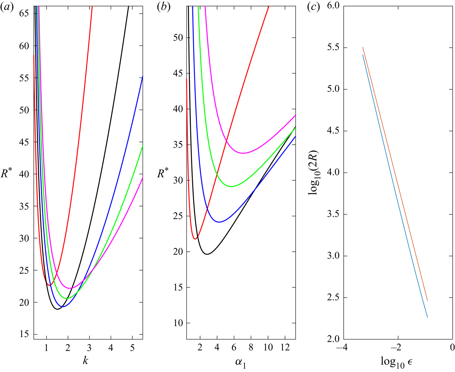
 $R^*$ is sufficiently large, and panel (a) of figure 1 shows a number of neutral curves in the
 $k$–
 $R^*$ plane for different values of
 $\alpha _1$ whilst panel (b) shows results at a fixed
 $k$. We note the branches of panel (a) approach infinity more quickly because of the asymptotic dependence on
 $\alpha _1, k$ just discussed. Our calculations found that the minimum
 $R^*=18.85$ occurs when
 $\alpha _1=2.224, k=1.58$. Floryan (Reference Floryan2002) gave the curve fit
 $\log (2 R) \simeq -1.2801 \log \epsilon +2.29539.$ Note that Floryan's Reynolds number is twice that used here. Our prediction has the 1.2801 replaced by 1.5, but the logarithmic factor in the denominator of (3.2) compensates for the slight mismatch in powers and in panel (c) of figure 1 we compare the two predictions. We see that there is good agreement between (3.2) and the formulae Floryan inferred from his numerical results. The most dangerous wavenumber in the limit of small
 $\epsilon$ given by Floryan also agrees with our predictions above.
Plane Couette flow results. The red, black, blue, green and magenta curves in (a,b) denote neutral curves in the  $k$–
 $R^*$ plane for
 $\alpha _1=1,2,3,4,5$ and in the
 $\alpha _1$–
 $R^*$ plane for
 $k=1,2,3,4,5$, respectively. Panel (c) compares asymptotic predictions of present theory (blue) with the red curve using the fit in Floryan (Reference Floryan2002).

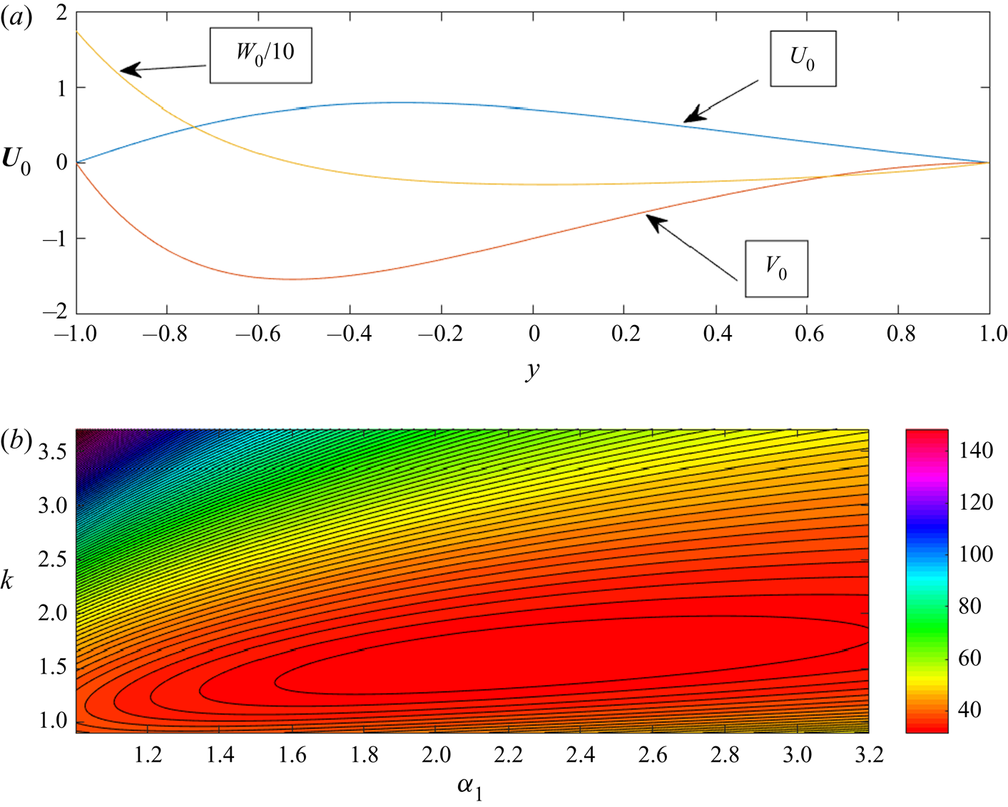
Figure 2 shows the neutral eigenfunctions  $U_0, V_0, W_0$ at
 $\alpha _1 = k = 2.$ and these agree well with the corresponding functions in Floryan (Reference Floryan2002). For the sake of brevity we do not give plots of the growth rates for non-neutral mode but they are also consistent with Floryan's results. Thus for example in figure 2 of Floryan (Reference Floryan2002) the orientation of the contours of constant growth rate is due to the different large and small behaviours of
 $R^*$ as the two wavenumbers vary; see panel (b) of figure 2 which shows curves of constant
 $R^*$ in the
 $\alpha _1, k$ plane.
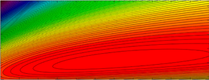
Panel (a) shows the neutral eigenfunctions  $U_0, V_0, W_0$ as functions of
 $y$ for
 $\alpha _1, k = 2.2$. Panel (b) shows contours of constant neutral values of
 $R^*$ in the
 $\alpha$–
 $k$ plane.

3.2. Poiseuille flow
Now consider the case when the flow is driven by a pressure gradient, in particular suppose that the flow is of the meandering type so that  $F=G=2\cos \alpha _1 x$. Note that our previous analysis showed that the relative phases of the walls is not important so our results also apply to the case when
 $G=2\cos \alpha _1(x+\phi )$ where
 $\phi$ is a constant. In fact the analysis applies even when the wall wavelengths differ since the vortex–wave interaction driving the instability is confined to wall layers. If there are now undulations on both walls two possible solutions exist but the fact that the unperturbed flow is even in
 $y$ shows that the two possibilities correspond to
 $U_0$ even or odd in
 $y$. Solution of the eigenvalue (2.23)–(2.27) for the even case yields
 \begin{align} R^*=\frac{3( \alpha^2_1+k^2)\left(k+\dfrac{\sinh 2k}{2}\right)}{ 2^{{1}/{3}}5 \alpha_1^{{4}/{3}} \textrm{Ai}' (0)^2\! \left[\!-\dfrac{3 \sinh2k}{2k}-3+\dfrac{3}{k} \coth k\cosh 2k+2k\coth k-\dfrac{3}{2k^2} (1+\cosh2k)\!\right]}, \end{align}
and a similar expression can be derived for the odd mode.
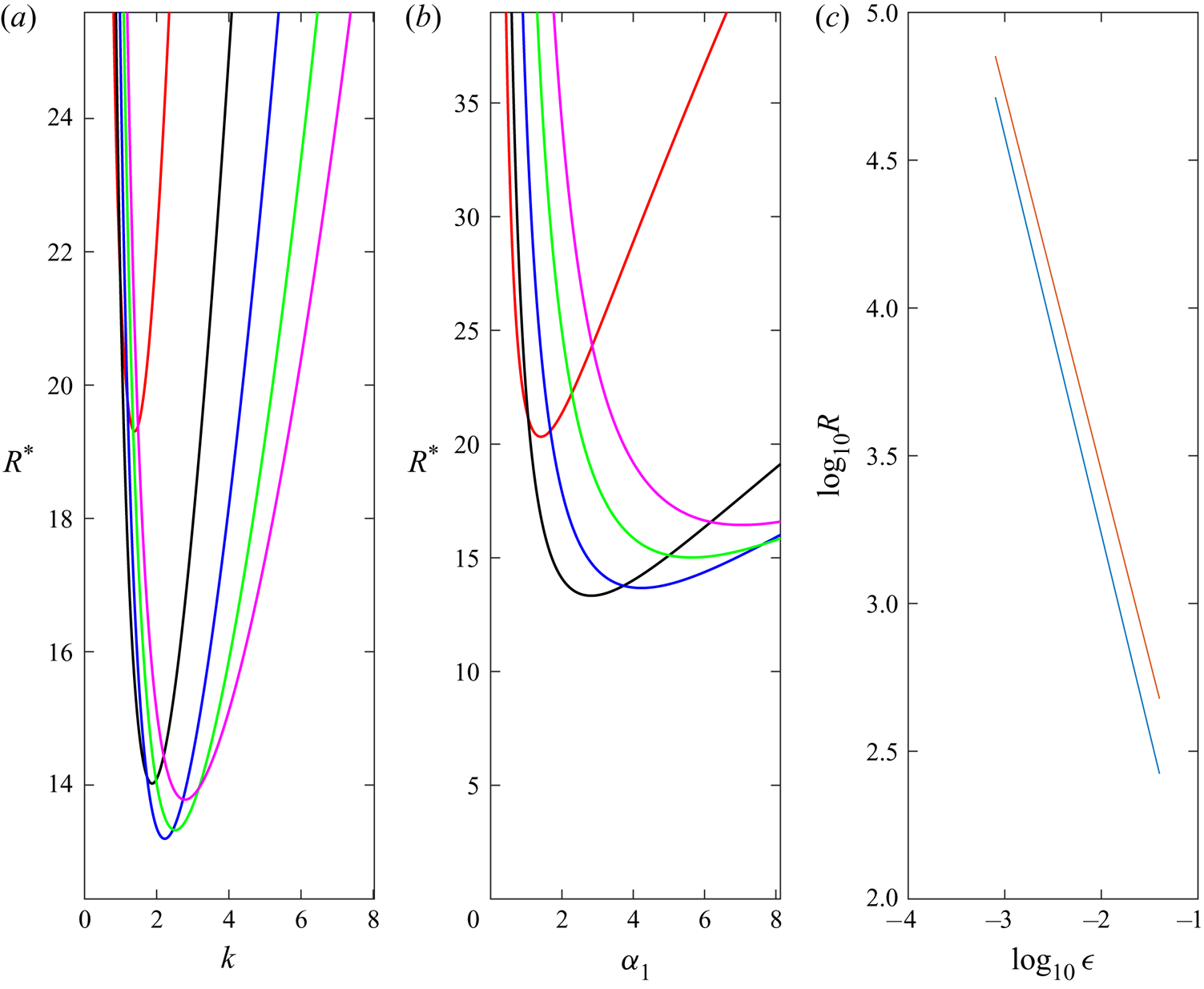
Both neutral curves have the same properties as the neutral curves for Couette flow for small and large wavenumbers. The most dangerous even and odd modes correspond to  $(\alpha _1, k, R^*) =(3.234, 2.29, 13.18), (3.85, 2.73, 14.38)$, respectively. Figure 3 shows the dependence of the Reynolds number
 $R$ as a function of the amplitude
 $\epsilon$ for the most dangerous mode. Also shown in the plot are results from Floryan (Reference Floryan2015). Once again the agreement between the asymptotic theory and the numerical study is good. The other mode is more stable and has a neutral curve displaced slightly upwards from the one shown, that is consistent with Floryan (Reference Floryan2003, Reference Floryan2015).
Plane Poiseuille flow results. The red, black, blue, green and magenta curves in (a,b) denote neutral curves in the  $k$–
 $R^*$ plane for
 $\alpha _1=1,2,3,4,5$ and in the
 $\alpha _1$–
 $R^*$ plane for
 $k=1,2,3,4,5$, respectively. Panel (c) compares asymptotic predictions of present theory (blue) with the red curve taken from Floryan (Reference Floryan2015).

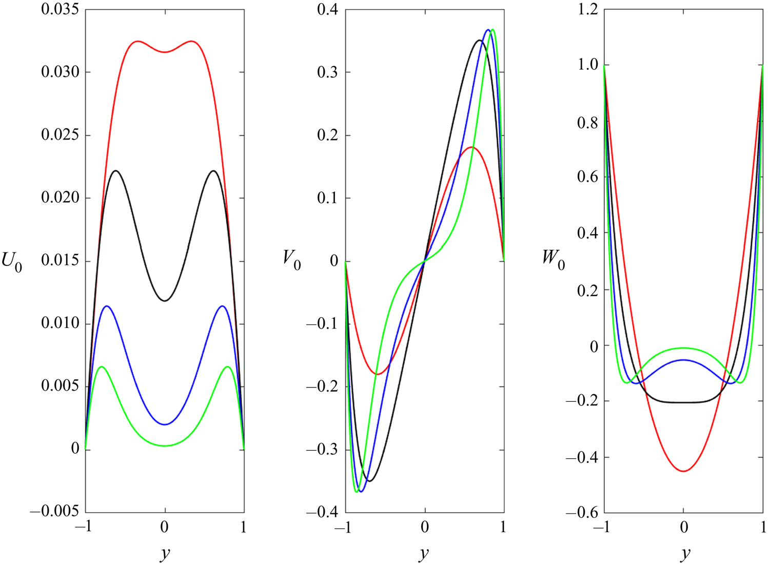
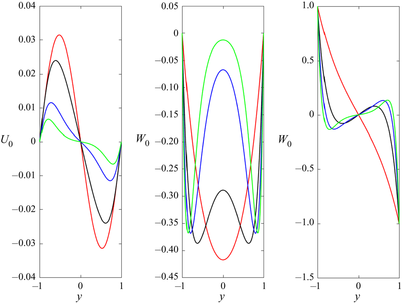
Figures 4 and 5 show the eigenfunctions  $U_0,V_0,W_0$ for
 $k=1,3,5,7$ for the even and odd modes, respectively. We have normalised the eigenfunctions such that
 $W_0(-1)=1$ in both cases and we see that as
 $k$ increases the eigenfunctions concentrate closer to the boundaries and it is easy to show that for large
 $k$ the concentration is in layers of thickness
 $O(k^{-1})$ at the walls. For progressively smaller values of
 $k$ we can derive simple expressions for the eigenfunctions and the
 $k=1$ results shown in figures 4 and 5 are already displaying that behaviour.
Eigenfunctions for the even mode in plane Poiseuille flow with  $k=1,3,5,7$ corresponding to the red, black, blue and green curves, respectively.

Eigenfunctions for the odd mode in plane Poiseuille flow with  $k=1,3,5,7$ corresponding to the red, black, blue and green curves, respectively.

4. Conclusion
The instability mechanism described here should not be confused with receptivity mechanisms. The latter describe the initiation of fluid instabilities by roughness and/or flow unsteadiness whereas here the roughness is itself part of the instability mechanism. Although we have described the instability in the context of fully developed channel flows, it is expected that the mechanism applies to developing flows with non-parallel effects taken into account asymptotically.
The instability is generated within the viscous wall layer in high Reynolds number flows and so undulations on the upper and lower walls act independently. At a given large value of the Reynolds number when the wall amplitude  $\epsilon$ is increased from zero the instability occurs before the size at which the wall layer associated with the basic flow becomes interactive. For walls with the same amplitude and wavelength the phase difference between the wall undulations has no effect on the instability. This explains why the results of the numerical investigations of stationary disturbances in meandering and converging/diverging channels by Floryan (Reference Floryan2003, Reference Floryan2015) appear somewhat indistinguishable. The agreement shown in figures 1 and 3 with Floryan's numerical investigations is, we believe, good given that the next order-correction to the neutral curves will be of relative size
 ${1}/{\log R}$. The eigenfunctions calculated are also consistent with Floryan's results.
The asymptotic approach can be used with walls having different amplitudes and wavelengths and the neutral configuration written down in closed form. The theory developed above can be applied to walls containing more than one wavelength and so by Fourier analysis it can be sensibly used to model rather arbitrary but small wall roughness. For roughness of fixed amplitude then as the Reynolds number is increased the wall wavelength corresponding to the most unstable mode will dominate and other wavelengths will not amplify structures at their wavelengths. Previous investigators have classified the instability as a centrifugal one associated with wall curvature. However, we believe that classification is not appropriate because we cannot use Rayleigh's argument about the motion of a displaced fluid particle in a curved flow to deduce instability. It is therefore perhaps more appropriate to think of the instability described here as a parametric instability or a ‘long wave/short wave’ instability.
The instability described here occurs at progressively higher Reynolds numbers as the wall wavelength approaches zero so that in the lubrication theory regime discussed in Gajjar & Hall (Reference Gajjar and Hall2020) it does not occur at finite values of the modified Reynolds numbers where the most dangerous mode takes on a quite different structure. The instability described here for channel flows will dominate when  $\epsilon$ is sufficiently large that its critical Reynolds number is less than that for Tollmien–Schlichting waves. The likely importance of the instability would be even higher if it turns out to be an absolute rather than a convective instability.
Acknowledgements
The author wishes to thank the referees for their constructive comments. This work was supported by the grant ARC-DP170104703.
Declaration of interests
The authors report no conflict of interest.