





Non-technical Summary
Understanding how animal communities responded to past environmental changes can help us predict how modern ecosystems might change in the future. In our study, we examined six extinct mammal communities from eastern Oregon, covering the past 32 million years. We collected information on what kinds of animals were present, what they likely ate, and how big they were. We used this information to reconstruct potential food webs of functional groups, which represent who was likely eating whom during that moment in time. We found some evidence that community composition changed in response to climate shifts, such as the warming and wet conditions of the mid-Miocene Climatic Optimum (about 16 million years ago) and later cooling events. These patterns were like those found elsewhere in North America. We also found that immigration events from the Eurasian continent also influenced Oregon mammalian functional diversity through time. The food webs revealed patterns that simple species lists or group counts alone could not show. For example, some communities had long and complex feeding chains and contained many omnivores and predators, which created a dense network of links between groups of organisms. Other communities were simpler and had groups of organisms that were not linked as strongly. Changes in the distribution of predators and omnivores in the community impacted the structure of the food webs, which suggests that shifts in their diversity through time may impact community stability and function. By looking at both the community structure from traits and the estimated food webs, we gained a clearer picture of how ancient Oregon ecosystems changed over time.
Introduction
Studies of past diversity dynamics provide important insights into how changes to our planet’s climate and environments can restructure animal communities. For example, large organisms are currently disappearing from the landscape, and the end-Pleistocene extinction provides a forecast of what the consequences of those continued disappearances might be (Ripple et al., Reference Ripple, Newsome, Wolf, Dirzo and Everatt2015). Another recent and equally important moment in Earth’s past was the community change that occurred during the Oligo-Miocene interval. Mammal communities transitioned to those that more closely resemble today’s modern communities (Figueirido et al., Reference Figueirido, Janis, Pérez-Claros, De Renzi and Palmqvist2012). During this time, the world saw the development and global expansion of grass-dominated habitats (Strömberg, Reference Strömberg2011) and dramatic shifts in terrestrial community composition (Figueirido et al., Reference Figueirido, Janis, Pérez-Claros, De Renzi and Palmqvist2012). The North American fossil record preserves this period well and captures browser diversity declining in both ungulates (Janis et al., Reference Janis, Damuth and Theodor2000, Reference Janis, Damuth and Theodor2002, Reference Janis, Damuth and Theodor2004) and rodents (Samuels and Hopkins, Reference Samuels and Hopkins2017). The herbivory shift during the Oligo-Miocene interval highlights how changes in vegetation and climate can select against certain functional groups and alter ecological communities.
Region-specific studies have added to this picture by investigating the variability in North American grassland expansion and the resulting community composition change over the past 20 million years. Most work has focused on the Great Plains (Stegner and Holmes, Reference Stegner and Holmes2013; Kita et al., Reference Kita, Secord and Boardman2014), the onset of C4 grasses (Feranec and Pagnac, Reference Feranec and Pagnac2013; Kita et al., Reference Kita, Secord and Boardman2014), or large herbivore ecology (Feranec and MacFadden, Reference Feranec and MacFadden2006). Local environmental factors influenced change (Chen et al., Reference Chen, Smith, Sheldon and Strömberg2015) and contributed to the heterogeneity in the timing of grassland expansion (Strömberg, Reference Strömberg2011; Strömberg and Staver, Reference Strömberg and Staver2022).
The Oregon fossil record, especially east of the Cascades, records nearly 40 million years of faunal change, is well dated in studies that make use of the widespread volcanic deposits (McLaughlin et al., Reference McLaughlin, Hopkins and Schmitz2016; Maguire et al., Reference Maguire, Samuels and Schmitz2018; Mohr et al., Reference Mohr, Famoso, Samuels, Laib and Schmitz2025) and has had hundreds of specimens collected and thoroughly studied over the past 100 years (Fremd, Reference Fremd2010). As it is today, Oregon was topographically complex and in a climatic zone that favored C3 plants over C4 plants (Ehleringer and Cerling, Reference Ehleringer, Cerling, Mooney and Canadell2002; Reuter et al., Reference Reuter, Wainwright, Hoffman, Clementz, Blumenthal and Hopkins2025) during the Oligo-Miocene, making it substantially different from many of the other regions that have been previously studied. For example, during the Oligo-Miocene, the Cascades Mountains were uplifted (Kohn and Fremd, Reference Kohn and Fremd2007; Bershaw et al., Reference Bershaw, Cassel, Carlson, Streig and Streck2019; Pesek et al., Reference Pesek, Perez, Meigs, Rowden and Giles2020; Kukla et al., Reference Kukla, Ibarra, Rugenstein, Gooley, Mullins, Kramer, Moragne and Chamberlain2021), the Columbia River flood basalts were deposited (Reidel et al., Reference Reidel, Camp, Ross, Wolff, Martin, Tolan and Wells2013; Cahoon et al., Reference Cahoon, Streck, Koppers and Miggins2020), and Basin and Range extension propagated into the state (Dickinson, Reference Dickinson2002). It has been hypothesized that the combination of these geological events and climate fluctuations during the Miocene increased habitat diversity and, therefore, species richness in Oregon (Kohn and Fremd, Reference Kohn and Fremd2007). This hypothesis aligns with work on modern and fossil assemblages that have shown that areas with complex topography have higher species richness because they provide a higher variety of habitats (Barnosky and Carrasco, Reference Barnosky and Carrasco2002; Badgley, Reference Badgley2010; Badgley et al., Reference Badgley, Smiley, Terry, Davis and DeSantis2017; Loughney et al., Reference Loughney, Badgley, Bahadori, Holt and Rasbury2021; Smiley et al., Reference Smiley, Bahadori, Rasbury, Holt and Badgley2024).
Paleosol evidence suggests that during the mid-Miocene Climatic Optimum (MMCO), a particularly warm interval ~16 Ma, Oregon received more rainfall than the Great Plains (Bestland et al., Reference Bestland, Forbes, Krull, Retallack and Fremd2008). Additional work has shown that the percentage of grass phytoliths in the Great Plains sedimentary record dramatically increased between 26 and 15 Ma (Kukla et al., Reference Kukla, Rugenstein, Ibarra, Winnick, Strömberg and Chamberlain2022), with phytolith composition indicating a mix of grassy and wooded patches in the middle Miocene and greater dominance of grasses during the latest Miocene (Strömberg, Reference Strömberg2011). In contrast to the Great Plains, the western coast had densely forested areas and saw less of a change in winter precipitation during the Miocene (Kukla et al., Reference Kukla, Rugenstein, Ibarra, Winnick, Strömberg and Chamberlain2022). These environmental differences are also reflected in the terrestrial communities. For example, the late Miocene Rattlesnake Formation shows evidence of grasslands and semiarid wooded shrublands (Retallack et al., Reference Retallack, Tanaka and Tate2002) but also contains boreal taxa, beavers, and petrified wood, indicating forested habitats (Samuels and Cavin, Reference Samuels and Cavin2013). Taken together, this suggests that although the interior of North America underwent a major biome shift toward open grasslands, Oregon maintained a more complex landscape with mixed and wooded environments well into the late Miocene. The tectonic and climatic differences from other areas of North America make Oregon an ideal place to investigate Oligo-Miocene terrestrial community change as it will substantially add to our knowledge of this moment in time.
The sheer amount of paleoecological data available because of the continued work in the John Day Fossil Beds National Monument and other similarly aged fossil sites throughout Oregon allows for a closer look at community structure than ever before (Albright et al., Reference Albright, Woodburne, Fremd, Swisher, MacFadden and Scott2008; Fremd, Reference Fremd2010; Orcutt and Hopkins, Reference Orcutt and Hopkins2011; Maguire et al., Reference Maguire, Samuels and Schmitz2018; Orcutt et al., Reference Orcutt, Schmer, Lubisich, Abrams and Famoso2024; Mohr et al., Reference Mohr, Famoso, Samuels, Laib and Schmitz2025). For example, the wealth of data allows for tentative reconstructions of food-web interactions. Food webs are networks of feeding relationships that, when compared with one another, can link community-level changes to interspecific data (Beckerman et al., Reference Beckerman, Petchey and Warren2006); they allow for the testing of hypotheses beyond those that can be answered with richness/diversity estimates (Morales-Castilla et al., Reference Morales-Castilla, Matias, Gravel and Araújo2015). Although usually estimated for extant communities, reconstructed probable food webs of extinct communities have been shown to be a powerful tool for understanding past trophic relationships (Dunne et al., Reference Dunne, Williams, Martinez, Wood and Erwin2008; Dunne and Yeakel, Reference Dunne and Yeakel2015; Wooster et al., Reference Wooster, Middleton, Wallach, Ramp and Sanisidro2024), the impact of taphonomic biases in the fossil record (Shaw et al., Reference Shaw, Coco, Wootton, Daems, Gillreath-Brown, Swain and Dunne2021), community restructuring after extinctions/invasions (Wooster et al., Reference Wooster, Middleton, Wallach, Ramp and Sanisidro2024), and how communities responded to extinctions and perturbations (Roopnarine and Angielczyk, Reference Roopnarine and Angielczyk2015; Lozano et al., Reference Lozano, Mateos and Rodríguez2016).
Past trophic networks can be estimated using a synthesis of information from both known biotic interactions and inferred interactions from taxa traits. Very rarely are biotic interactions preserved in the fossil record; this is especially true for terrestrial vertebrates. Evidence such as food material preserved in coprolites represents one of the rare cases in which direct interactions are preserved (Hunt et al., Reference Hunt, Lucas, Milàn and Spielmann2012). When direct evidence is not available, dietary proxies provide the next backbone for inferring potential interactions. Ecomorphological data (Barr, Reference Barr2018), body-mass estimates (Carbone et al., Reference Carbone, Mace, Roberts and Macdonald1999; Reuter et al., Reference Reuter, Hopkins and Price2023), and observations from predator and prey relationships in modern ecosystems provide the basis for inferring probable links and impossible links (Morales-Castilla et al., Reference Morales-Castilla, Matias, Gravel and Araújo2015). In this way, food webs of varying levels of detail and confidence can be reconstructed for extinct communities by aggregating available ecological information for each taxon found in an assemblage (Dunne et al., Reference Dunne, Williams, Martinez, Wood and Erwin2008; Roopnarine, Reference Roopnarine, Alroy and Hunt2010; Dunne and Yeakel, Reference Dunne and Yeakel2015; Morales-Castilla et al., Reference Morales-Castilla, Matias, Gravel and Araújo2015; Roopnarine and Angielczyk, Reference Roopnarine and Angielczyk2015; Shaw et al., Reference Shaw, Coco, Wootton, Daems, Gillreath-Brown, Swain and Dunne2021). The hypotheses being tested will additionally determine what detail within the food web is needed and what food-web properties will be examined.
In addition, patterns in food-web properties, quantified through network metrics, have been linked to important processes that influence ecological communities. These network metrics, such as connectance (realized possible connections) and compartmentalization (degree of modularity), can also reflect differences in community composition across ecosystems (Briand and Cohen, Reference Briand and Cohen1987). For example, forested environments often harbor a higher diversity of omnivores and frugivores (Badgley and Fox, Reference Badgley and Fox2000), which may result in more trophic roles being filled and subsequently longer food chains (Briand and Cohen, Reference Briand and Cohen1987). Furthermore, a higher proportion of smaller carnivores has been associated with increased connectance in food webs (Beaudrot et al., Reference Beaudrot, Acevedo, Gorczynski and Harris2024). Forested or patchy habitats may also promote greater compartmentalization, or modularity, in which subgroups of species are more tightly linked to each other than to the rest of the network (Baskerville et al., Reference Baskerville, Dobson, Bedford, Allesina, Anderson and Pascual2011; Macfadyen et al., Reference Macfadyen, Gibson, Symondson and Memmott2011). These compartments can buffer ecosystems by limiting the spread of perturbations, potentially enhancing long-term ecological stability (Baskerville et al., Reference Baskerville, Dobson, Bedford, Allesina, Anderson and Pascual2011). By comparing food-web metrics across fossil assemblages from different environments and periods, we can evaluate how structural properties of ecosystems responded to past environmental change (Yeakel et al., Reference Yeakel, Pires, Rudolf, Dominy, Koch, Guimarães and Gross2014; Morales-Castilla et al., Reference Morales-Castilla, Matias, Gravel and Araújo2015) and faunal changes (Wooster et al., Reference Wooster, Middleton, Wallach, Ramp and Sanisidro2024).
In this study, we compiled the trophic and body-mass information of six fossil assemblages to evaluate functional diversity and differences in potential trophic guild web structure for each fossil assemblage. We aimed to answer the following questions: (1) how has Oregon mammalian community structure changed over the past 32 Myrs; (2) are differences in community structure driven by particular trophic strategies; (3) do the changes in functional diversity and trophic structure align with our current knowledge of ecosystem change in Oregon?
Methods
Geological setting
This study focused on five well-collected and well-dated Oregon fossiliferous geologic units: The John Day Formation Turtle Cove Member (~32 to 26 Ma; Fisher and Rensberger, Reference Fisher and Rensberger1972; Albright et al., Reference Albright, Woodburne, Fremd, Swisher, MacFadden and Scott2008; Mohr et al., Reference Mohr, Famoso, Samuels, Laib and Schmitz2025), the Mascall Formation (~16 to 13 Ma; McLaughlin et al., Reference McLaughlin, Hopkins and Schmitz2016; Maguire et al., Reference Maguire, Samuels and Schmitz2018), the Juntura Formation (~12.5 to 9.5; Hooper et al., Reference Hooper, Binger and Lees2002; Camp et al., Reference Camp, Ross and Hanson2003), the Rattlesnake Formation (~7.3 to 6.9 Ma; Streck and Grunder, Reference Streck and Grunder1995; Prothero et al., Reference Prothero, Hoffman and Foss2006) and the McKay Formation (~6 to 5.5 Ma; Martin et al., Reference Martin, Hargrave and Ball2018). The Turtle Cove Member is informally split into faunally distinct upper and lower units above and below the Picture Gorge Ignimbrite, which has been dated to 29 Ma (Mohr et al., Reference Mohr, Famoso, Samuels, Laib and Schmitz2025). These formations document the environmental change that occurred in Oregon as global temperature fluctuated through the Oligo-Miocene (Fig. 1).
Stratigraphic and age context of formations included in this study. Red line represents the Benthic δ18O from Westerhold et al. (Reference Westerhold, Marwan, Drury, Liebrand and Agnini2020), which documents changes in deep ocean temperature. Map of Oregon indicates the geographic area of the fossil localities included in this study.

Figure 1. Long description
The left panel features a vertical line graph and stratigraphic column. The Y-axis represents time in Millions of years ago, ranging from 32 at the bottom to 5 at the top. The X-axis at the top measures Benthic delta 18 O per mil, ranging from 2 to 3.5. A thick red line fluctuates vertically, showing a sharp increase in delta 18 O around 16 million years ago. The stratigraphic column is divided into three epochs from bottom to top: Oligocene (32 to 23 million years ago), Early Miocene (23 to 16 million years ago), Mid Miocene (16 to 11 million years ago), and Late Miocene (11 to 5 million years ago).
In the center, six boxes label specific geological formations, with lines connecting them to the stratigraphic timeline and to specific points on the map to the right. From top to bottom, these are:
- McKay Formation (Late Miocene)
- Rattlesnake Formation (Late Miocene)
- Juntura Formation (Late Miocene)
- Mascall Formation (Mid Miocene)
- John Day Formation upper Turtle Cove Member (Oligocene)
- John Day Formation lower Turtle Cove Member (Oligocene)
The right panel is a map of Oregon showing county lines and major cities: Eugene, Bend, and John Day. Black dots representing fossil localities are concentrated in the central and eastern regions of the state. Lines from the formation boxes point to these dots, indicating their geographic distribution. The Mascall Formation points to two locations in central Oregon, while the McKay and Juntura formations point to locations further East.
Obtaining occurrence and ecological data
Faunal occurrences for the formations were compiled from the Paleobiology Database (paleobiodb.org) with additional information from the John Day Fossil Beds National Monument collections (JODA) and published formation descriptions (Maguire et al. Reference Maguire, Samuels and Schmitz2018; Orcutt and Hopkins, Reference Orcutt and Hopkins2011; Orcutt et al., Reference Orcutt, Schmer, Lubisich, Abrams and Famoso2024). Body mass was reconstructed for each extinct taxon using m1 area and regressions from Legendre (Reference Legendre1986; see Supplemental data 1 for equations used). We chose to use m1 measurements for body-mass estimation because it is the most common element that could be used for all taxa included in this study. Data for m1 area were compiled from the Paleobiology Database with additional information from published descriptions (see Supplemental data 2 for all measurement references). If a species’ m1 was not available, comparisons with other members of the genus were used to estimate mass using another species’ measurement or a genus average. Some rare species unique to these formations have no other member of their genus and are missing an m1 measurement; their body mass was therefore interpreted from their original descriptions (e.g., Watay tabutsigwii McLaughlin et al., Reference McLaughlin, Hopkins and Schmitz2016).
Diet data for extinct species were collected from both the Paleobiology Database and, when more detail was needed, primary literature reviews (see Supplemental data 5 for references). The literature reviews drew from studies that included diet inferred from dental morphology, microwear, and mesowear. Species’ diets were then categorized using seven dietary categories: carnivory, insectivory, omnivory, and herbivory, with herbivores further subdivided into browsers, grazers, and mixed feeders.
To compare our data with the modern Oregon mammalian community, we also compiled information on the extant mammals currently living in the John Day region using a similar protocol. Extant mammal species occurrences were downloaded from the IUCN via a polygon centered on the John Day River Basin (IUCN, 2017). Bats and human-associated commensal mammals were removed because they are rarely preserved in the fossil assemblages of this study. Body masses and diet categories for extant animals were compiled from the PanTHERIA Database (Jones et al., Reference Jones, Bielby, Cardillo, Fritz and O’Dell2009), and we used primary literature sources, such as species accounts, when data were not available through PanTHERIA or when further description was needed to determine the herbivorous diet type.
On initial comparison, we noted that the modern assemblage had a high number of small omnivorous taxa compared with the fossil localities. Studies that include soft-tissue data make it possible to obtain precise diets for extant small mammal species, making it easier to detect omnivorous diets. For example, the coast mole in the modern John Day dataset (Scapanus orarius True, Reference True1896) is classified as an omnivore due to its stomach contents, which were noted by Whitaker et al. (Reference Whitaker, Maser and Pedersen1979) to have plant material. It is impossible to get the same diet resolution for extinct species. In addition, many diets reported for taxa in the Paleobiology Database are assumed from family-level or order-level trends. Thus, extinct members of the families Sciuridae, Heteromyidae, Cricetidae, and Soricidae were reassigned from herbivory, the state given in the Paleobiology Database, to omnivory, which aligns with extant family diet data (Reuter et al., Reference Reuter, Hopkins and Price2023). The final dataset was then used in all analyses. All analyses and visualizations were performed using the statistical program R (R Core Team, 2024).
Functional diversity
To understand the functional structure of these formations and how they changed through time, taxa for each formation were divided into body-mass and diet-informed functional categories: extra-large herbivore (>44 kg, EH); large herbivore (8–44 kg, LH); medium herbivore (0.5–8 kg, MH); small herbivore (<0.5 kg, SH); large carnivore (>8 kg, LC); medium carnivore (0.5–8 kg, MC); small carnivore (<0.5 kg, SC); large omnivore (>8 kg, LO); medium omnivore (0.5–8 kg, MO); small omnivore (<0.5 kg, SO); medium insectivore (0.5–8 kg, MI); small insectivore (<0.5 kg, SI). These categories have been shown in the past to differ between environments and through time (Legendre, Reference Legendre1986; Barnosky and Shabel, Reference Barnosky and Shabel2005; Stegner and Holmes, Reference Stegner and Holmes2013).
We then compared the distribution of functional groups in each fossil assemblage using a correspondence analysis from the FactoMineR package (Lê et al., Reference Lê, Josse and Husson2008). In addition, pairwise Fisher’s exact tests with Monte Carlo p-value simulations (5,000 replicates) were performed to compare the distribution of functional groups between assemblages. All p-values were then adjusted using Holm p-value adjustment for multiple comparisons. This approach follows those of Stegner and Holmes (Reference Stegner and Holmes2013), who used similar methods to detect differences in Great Plains extinct communities.
Food-web reconstruction and analyses
To complement the functional diversity comparisons and to understand the trophic structure of the communities, food webs were reconstructed for each fossil assemblage. Individual plant and invertebrate species were not included as our goal was to see how the mammalian community structure changed. In addition, the invertebrate and paleobotanical records for many of these formations are incomplete, and aligning these records between each formation was beyond the scope of this project. As such, the food webs in this study represent probable links in a certain time and place among functional mammalian groups and their connections to the generalized base nodes of browse, grass, and invertebrates.
Potential community links were reconstructed using the collected body-mass data and dietary information for each taxon, along with the prey and predator body-mass relationships found in Table 1. These size–class relationships are not an exact prediction of prey and instead serve as a basis for reconstructing possible interactions while excluding impossible or highly unlikely interactions. Reconstructing theoretical networks of ecological interactions using trait information and body-mass relationships is a common approach for both extinct (Yeakel et al., Reference Yeakel, Pires, Rudolf, Dominy, Koch, Guimarães and Gross2014; Roopnarine and Angielczyk, Reference Roopnarine and Angielczyk2015) and modern communities (Beaudrot et al., Reference Beaudrot, Acevedo, Gorczynski and Harris2024) and aligns with the suggested framework of Morales-Castilla et al. (Reference Morales-Castilla, Matias, Gravel and Araújo2015) for inferring biotic interactions for ecological networks.
Body-mass rules used to reconstruct potential predator–prey relationships

Table 1. Long description
The table consists of four columns: Predator size class, Example, Sizes consumed, and Example.
* Row 1: Predators less than 4.5 kg (e.g., Martes americana) consume prey less than 2 kg (e.g., Neotoma cinerea).
* Row 2: Predators between 4.5 and 10.0 kg (e.g., Taxidea taxus) consume prey less than 4.5 kg (e.g., Lepus americanus).
* Row 3: Predators greater than 10.0 to 21.5 kg (e.g., Canis latrans) consume prey less than 9.5 kg (e.g., Erethizon dorsatum).
* Row 4: Predators greater than 21.5 to 45.0 kg (e.g., Canis lupus) consume prey between 9.5 and 120 kg (e.g., Odocoileus virginianus).
* Row 5: Predators greater than 45.0 kg (e.g., Puma concolor) consume prey greater than 9.5 kg (e.g., Cervus canadensis).
We based the body-mass relationships used in this study (Table 1) on documented predator–prey observations from modern ecological communities and metabolic-related constraints outlined in previous studies (Carbone et al., Reference Carbone, Mace, Roberts and Macdonald1999; Sinclair et al., Reference Sinclair, Mduma and Brashares2003; Owen-Smith and Mills, Reference Owen-Smith and Mills2008). In modern ecosystems, predators of certain size classes specialize on prey of predictable mass because of handling constraints and different energetic costs and benefits of hunting that prey (Carbone et al., Reference Carbone, Mace, Roberts and Macdonald1999; Sinclair et al., Reference Sinclair, Mduma and Brashares2003; Owen-Smith and Mills, Reference Owen-Smith and Mills2008). For example, Carbone et al. (Reference Carbone, Mace, Roberts and Macdonald1999) found that predators weighing under 21.5 kg tend to eat invertebrates and prey weighing 45% or less of the predator’s body mass, whereasile predators weighing over 21.5 kg eat prey 45% or more of the predator’s body mass. This transition at 21.5 kg reflects a shift in energetic needs and is grounded in metabolic scaling that is broadly conserved among mammalian carnivores (Carbone et al. Reference Carbone, Mace, Roberts and Macdonald1999) and omnivores (Reuter et al., Reference Reuter, Hopkins and Price2023). In addition, evidence from Serengeti ecosystems suggests that predator diets exhibit a nested scaling structure, where smaller carnivores consume a narrow prey-size range and larger carnivores consume a broader range that includes smaller prey opportunistically (Sinclair et al., Reference Sinclair, Mduma and Brashares2003). Therefore, body-mass relationships found in Table 1 are generous compared with those recorded for communities in Africa and define feasible prey mass ranges rather than deterministic prey assignments. Furthermore, for this study, predator behavioral details such as pack hunting were not assumed for link reconstruction, but our body-mass rules are based on many modern relationships that include species that exhibit pack hunting. We are aware that some of these predator behaviors have arisen only in very recent times (Janis and Wilhelm, Reference Janis and Wilhelm1993), and pack hunting has been suggested to allow smaller predators to kill prey much larger than themselves (Griffiths, Reference Griffiths1980). Therefore, using modern predator–prey relationships that include pack-hunting prey-size advantages would slightly overestimate the maximum size of prey for some Oligo-Miocene carnivores. However, increases in maximum prey size consumed have not been found for every pack-hunting species as this behavior also offers other non-prey-size-related advantages that may be a stronger influence on the evolution of this behavior (Lamprecht, Reference Lamprecht1981; Schmidt and Mech, Reference Schmidt and Mech1997). So it is reasonable to infer that body-size relationships between predators and prey were not fundamentally reorganized by this behavioral change exhibited in a few lineages given that mammalian body size in predator and prey species has been fairly consistent through time since the Oligocene (Smith and Lyons, Reference Smith and Lyons2011).
In addition to the predator body-mass relationships found in Table 1, we removed additional unrealistic links, which is also a recommended step in the framework suggested for inferring biotic interactions for ecological networks (Morales-Castilla et al., Reference Morales-Castilla, Matias, Gravel and Araújo2015). For example, in the initial link reconstruction, carnivores were allowed to prey on other carnivorous species as it is a common behavior to show aggression and kill smaller competitors, thus regulating the population sizes of smaller predators (Roemer et al., Reference Roemer, Gompper and Van Valkenburgh2009). However, we removed links where smaller carnivores were consuming larger carnivores; this has been done in other food-web reconstructions as smaller predators do not affect larger predator populations (Wooster et al., Reference Wooster, Middleton, Wallach, Ramp and Sanisidro2024). We also removed cannibalistic links as we are interested in structural guild relationships, and this behavior is not an important dietary source for most terrestrial mammals.
Furthermore, to account for differences in community preservation between the assemblages, the initial taxon-specific webs were then condensed into “trophic-species webs.” It is well known that the fossil record is incomplete. Time-averaging and taphonomic processes can affect preserved community structure and richness. Link-based aggregation is a common practice in ecological network studies as it can help reduce sampling differences and is useful for studying community-level patterns across environmental gradients and through time (Shaw et al., Reference Shaw, Coco, Wootton, Daems, Gillreath-Brown, Swain and Dunne2021; Gauzens et al., Reference Gauzens, Thouvenot, Srivastava, Kratina and Romero2025). For each food web, we therefore collapsed all nodes that have identical relationships in the web into a “trophic species” node that represents a functional role in the community. The resulting web represents plausible links between functional groups and not necessarily links between individual taxa within a fossil assemblage.
Next, for each reconstructed trophic-species web, we calculated some commonly used network metrics. The metrics used, their definitions, and which package was used for each metric can be found in Table 2. These metrics were selected because of our interest in understanding whether environmental differences caused network structure differences through time in Oregon.
Metrics used in this study

Table 2. Long description
The table is organized into three columns: Metric type, Metric, and Definition.
Network-level metrics include:
* Trophic species (S): Number of nodes in the trophic species web.
* Number of links (L): Total number of trophic interactions.
* Link density (L/S): Average number of links per node (L/S).
* Connectance (C): Realized proportion of all possible links (L/S super 2).
* Compartmentalization (Comp): Degree of modularity in the network (distinct subgroups).
* Characteristic path length (C P L): Average of the shortest path between all node pairs.
Node-level metrics include:
* Mean trophic level (T L): Average trophic level (T L) across all nodes (T L = 1 + mean(T L of the node’s resources)).
* Max trophic level (T L): Highest trophic level observed in the network.
* Trophic level S D: Standard deviation of trophic levels across all nodes.
* Omnivory fraction: Proportion of consumers feeding across multiple trophic levels (defined here as S D of prey T L greater than or equal to 0.5); this reflects dietary breadth across the food-web hierarchy, identifying nodes with vertically diverse diets.
Note: These were calculated in R using either the cheddar package (Hudson et al., Reference Hudson, Emerson, Jenkins, Layer, Ledger, Pichler, Thompson, O’Gorman, Woodward and Reuman2013) or the igraph package (Csardi and Nepusz, Reference Csardi and Nepusz2006).
In addition, because body mass is one of the primary traits guiding our food-web reconstruction, we evaluated the sensitivity of inferred network structure to uncertainty in dental-based mass estimations. We used a Monte Carlo framework and propagated body-mass uncertainty through the full food-web reconstruction pipeline described above. In each Monte Carlo replicate, each taxon’s estimated body mass was treated as the geometric mean of a lognormal distribution and randomly resampled from that distribution. The spread of the lognormal distribution was controlled by a coefficient of variation (CV), with values of 10%, 20%, and 30%. These CV values were converted to the corresponding log-scale standard deviation used to produce the distribution around the estimated body mass. A body mass was then randomly sampled from these distributions for each taxon. The taxa and their sampled masses were then propagated through the full reconstruction pipeline, including predator/prey size-class assignment, removal of unrealistic links, trophic-species aggregation, and network metric calculation. We did this 1,000 times per assemblage at three uncertainty levels (CV = 10%, 20%, 30%), resulting in 3,000 trophic-species webs and their associated metrics per assemblage. We then performed a principal components analysis (PCA) of the metric results to visualize food-web and community differences. Finally, to evaluate differences in overall food-web structure among formations, we performed a permutational multivariate analysis of variance (PERMANOVA; Anderson, Reference Anderson2001) on the resulting Monte Carlo dataset. Because each Monte Carlo simulation propagated uncertainty in body-mass estimates through the entire food-web reconstruction process, the PERMANOVA tested whether multivariate food-web structure differed among formations despite uncertainty in body-mass estimation and inferred trophic links. Before analysis, all network metrics were standardized (mean = 0, SD = 1) to account for differences in measurement scales. For the analysis, Euclidean distances were chosen as the distance measure, and statistical significance was assessed using 1,000 permutations. See Supplemental data 3 and 4 for the code for all analyses and Supplemental data 5 for the dataset used in reconstructing the trophic links.
Repositories and institutional abbreviations
Specimens used in this study are housed in the following institutions: University of Oregon Museum of Natural and Cultural History (UOMNH), Eugene, Oregon, USA; John Day Fossil Beds National Monument (JODA), National Park Service, Kimberly, Oregon, USA.
Results
Functional diversity
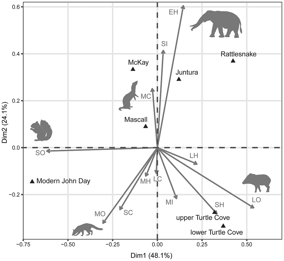
Diet and body-mass distributions for each faunal assemblage can be found in Figure 2, and a contribution plot from the correspondence analyses (CA), which displays the relative influence of each functional group, can be found in Figure 3. Raw functional group occupation counts can be found in Supplemental data 6.
Diet and body-mass distribution beeswarm plots for each faunal assemblage. B = browsers; M = mixed-feeding herbivores; G = grazers; O = omnivores; C = carnivores; I = insectivores. Colors also correspond to functional groups.

Figure 2. Long description
A multi-panel set of seven beeswarm plots. Each plot shares a y-axis representing the natural log of body mass in kilograms, ranging from negative 5 to 10. The x-axis categorizes functional groups as B for browsers, M for mixed-feeding herbivores, G for grazers, O for omnivores, C for carnivores, and I for insectivores.
Top row from left to right:
* Juntura approximately 12.5 to 9.5 millions of years ago: Shows high density in B and O groups, with B spanning the full y-axis range and O concentrated between negative 5 and 5.
* Rattlesnake approximately 7.3 to 6.9 millions of years ago: Displays a sparse G group and a cluster of O and C groups between 0 and 7.
* McKay approximately 6 to 5.5 millions of years ago: Features a wide distribution in B and a dense cluster of O below 0.
* Modern John Day: Shows a very high density of O between negative 5 and 5, with a small cluster of C around 2.
Bottom row from left to right:
* lower Turtle Cove approximately 32 to 29 millions of years ago: Shows clusters in B, M, O, and C, with O and C being particularly dense between 0 and 5.
* upper Turtle Cove approximately 29 to 26 millions of years ago: Displays a vertical spread of O from negative 7 to 5 and a small cluster of C at 5.
* Mascall approximately 16 to 13 millions of years ago: Shows a high concentration of B between 0 and 10 and a dense O group between negative 5 and 5.
Across all plots, B is dark green, M is light green, G is yellow-green, O is purple, C is red, and I is pink.
Correspondence analysis contribution plot for each faunal assemblages, represented by black triangles. Gray lettering indicates functional group: EH: >44 kg herbivores; LH: 8–44 kg herbivores; MH: 0.5–8 kg herbivores; SH: <0.5 kg herbivores; LC: >8 kg carnivores; MC: 0.5–8 kg carnivores; SC: <0.5 kg carnivores; LO: >8 kg omnivores; MO: 0.5–8 kg omnivores; SO: <0.5 kg omnivores; MI: 0.5–8 kg insectivores; SI: <0.5 kg insectivores. The length and angle of gray arrows indicate the strength of their contributions to the dimensions.

Figure 3. Long description
The Correspondence analysis contribution plot uses D i m 1 on the x-axis (48.1 percent) and D i m 2 on the y-axis (24.1 percent).
* Top-Right Quadrant: Contains the Rattlesnake and Juntura assemblages. A long vector for E H (extra-large herbivores) points toward an elephant silhouette. A shorter vector for S I (small insectivores) points upward.
* Top-Left Quadrant: Contains McKay and Mascall assemblages. A vector for M C (medium carnivores) points toward a weasel silhouette.
* Bottom-Left Quadrant: Contains the Modern John Day assemblage. Vectors for S O (small omnivores), M O (medium omnivores), S C (small carnivores), and M H (medium herbivores) radiate outward. A squirrel silhouette is on the far left and a fox-like silhouette is at the bottom.
* Bottom-Right Quadrant: Contains upper Turtle Cove and lower Turtle Cove assemblages. Vectors for L H (large herbivores), S H (small herbivores), L O (large omnivores), L C (large carnivores), and M I (medium insectivores) radiate toward a peccary silhouette.
Assemblages are marked with black triangles, while functional groups are indicated by gray arrows originating from the center (0,0) point.
The reconstructed diet and body-mass distributions showed that the fossil communities differed in their composition of functional groups. In particular, herbivore functional diversity differed among the formations (Figs. 2, 3). The modern Oregon assemblage mostly consisted of mixed-feeding herbivores, whilereas many of the fossil localities have higher proportions of large-browsing taxa. The Mascall fauna stood out for having a diverse herbivore community, with the most size and diet categories filled and the largest proportion of extra-large browsers (body mass >44 kg). By contrast, the modern, Rattlesnake, and McKay communities had a lower proportion of browsers compared with the Mascall and Turtle Cove communities.
Omnivore distributions also revealed differences among assemblages. The Turtle Cove faunas and the Rattlesnake fauna were particularly distinct, containing higher numbers of large omnivores than the McKay, Juntura, Mascall, and modern communities. The lower Turtle Cove had the highest number of large omnivores (n = 14). These are mainly canids and tayassiuds, which were low in diversity or non-existent in the modern John Day community. The McKay, Juntura, Mascall, and modern communities had high numbers of small omnivorous taxa and lower numbers of large and medium omnivorous taxa. As discussed in Methods, the modern assemblage had the highest proportion of small omnivores (n = 32), and these consist mostly of mice and squirrels.
Carnivore composition was more evenly distributed between assemblages, although some differences were notable. The lower Turtle Cove had the smallest carnivorous species, setting it apart from the other formations, and the Mascall Formation contained carnivores with the largest reconstructed body masses (i.e., the amphicyonids Amphicyon, Cynelos, and Pliocyon). Both the lower Turtle Cove and the modern John Day community showed fairly even carnivore distributions, with species in all size classes, unlike the other communities.
The CA provided more details about the community differences. The first two dimensions cumulatively explained 72.3% of the variance among communities. Omnivores and extra-large herbivores contributed the most to this variance, and the functional groups closest to the plot origin, such as large carnivores and large herbivores, contributed very little to the variance. For example, the influence of extra-large herbivores and large omnivores appeared to drive the separation of the Rattlesnake Formation in CA space (Fig. 2). In addition, fossil assemblages from the same geological epochs are clustered in ordination space, suggesting that similarly aged assemblages have similar faunal distributions.
Pairwise Fisher’s exact tests with Holm-adjusted p-values indicated that three fossil assemblages are significantly different from the modern community: the lower Turtle Cove Member, the upper Turtle Cove Member, and the Rattlesnake Formation (p = 0.02 for all). These differences appeared to be driven primarily by the abundance of small and large omnivores in these assemblages, as indicated by their position in the CA contribution plot. No fossil assemblages were found to be significantly different from one another.
Food-web structure
Table 3 summarizes the median trophic network metric values for each faunal assemblage across all 3,000 replicates. These metrics include measures of size (e.g., number of trophic species and links), complexity (e.g., connectance and link density), energy flow (e.g., mean trophic level and omnivory), and modularity (compartmentalization). Further information regarding the resulting calculated metrics and their values at different CV distributions can be found in Supplemental data 7. Overall, the faunal assemblages varied in reconstructed food-web complexity. The lower Turtle Cove assemblage had the most complex food webs, with the highest number of trophic species (median = 34) and the most links (median = 279). The lower Turtle Cove also exhibited high median link density (median LD = 8.2), extensive omnivory (median TL Omn = 0.73), and high mean trophic levels (median mean TL = 3.4), reflecting diverse interconnected trophic-species webs. By contrast, the McKay assemblage had the second-fewest trophic species (median = 20) and the lowest median link density (median = 2.9). Furthermore, all networks were found to contain two modules, but the strength of compartmentalization in the webs varied (median compartmentalization ranged from 0.29 to 0.41), with the modern Oregon food web showing the weakest compartmentalization and Mascall the strongest, suggesting differences in how interactions were distributed between and within these two modules. One representative trophic-species food web for each assemblage can be found in Supplemental Figure S2.
Median food-web metrics calculated from trophic-species webs

Table 3. Long description
The table contains 11 columns: Faunal assemblage, S, L, L forward slash S, C, Comp, Mean T L, Max T L, S D T L, T L Omn fraction, and C P L.
* Modern Oregon: S 26, L 131, L forward slash S 5.04, C 0.19, Comp 0.29, Mean T L 2.95, Max T L 4.16, S D T L 1.04, T L Omn fraction 0.63, C P L 1.40.
* McKay: S 20, L 58, L forward slash S 2.9, C 0.15, Comp 0.34, Mean T L 2.38, Max T L 3.44, S D T L 0.74, T L Omn fraction 0.29, C P L 1.25.
* Rattlesnake: S 24, L 117, L forward slash S 4.84, C 0.20, Comp 0.33, Mean T L 2.78, Max T L 3.94, S D T L 0.96, T L Omn fraction 0.55, C P L 1.40.
* Juntura: S 18, L 65, L forward slash S 3.58, C 0.20, Comp 0.29, Mean T L 2.63, Max T L 3.97, S D T L 0.94, T L Omn fraction 0.50, C P L 1.40.
* Mascall: S 25, L 112, L forward slash S 4.44, C 0.17, Comp 0.41, Mean T L 2.69, Max T L 3.73, S D T L 0.86, T L Omn fraction 0.58, C P L 1.23.
* Upper Turtle Cove: S 25, L 147, L forward slash S 5.92, C 0.24, Comp 0.32, Mean T L 3.00, Max T L 4.47, S D T L 1.12, T L Omn fraction 0.62, C P L 1.46.
* Lower Turtle Cove: S 34, L 279, L forward slash S 8.24, C 0.24, Comp 0.36, Mean T L 3.43, Max T L 5.00, S D T L 1.24, T L Omn fraction 0.73, C P L 1.50.
Note: S = median number of trophic species; L = median number of links in food web; C = median connectance; Comp = median compartmentalization; TL = median prey averaged trophic level; CPL = median characteristic path length. See Table 2 for metric definitions.
PCA of the metrics can be found in Figure 4 and further shows the differences between the communities. The first two principal components together explained 92.1% of the variance (PC1 = 77.2%; PC2 = 15.0%). PC1 captured primarily food-web complexity, with positive loadings from compartmentalization (0.017) and negative loadings from mean trophic level (–0.36), link density (–0.35), and maximum trophic length (–0.35). PC2 described variation in how links are distributed in the web, contrasting highly modular networks with more structurally integrated webs. PC2 had positive loadings from CPL (0.33) and connectance (0.23) and strong negative loadings from compartmentalization (–0.78).
Principal components analysis (PCA) of food-web metrics calculated from reconstructed trophic-species food webs generated during the Monte Carlo body-mass sensitivity analysis. Gray arrows indicate the loadings of each food-web metric (descriptions of metrics can be found in Table 2). Colors represent faunal assemblages, and the colored points represent individual trophic-species food webs produced by Monte Carlo simulations of body-mass uncertainty. Ellipses represent 95% of data for each assemblage. Representative trophic-species food webs are shown in Supplemental Figure S2.

Figure 4. Long description
A scatter plot of P C A results with P C 1 on the horizontal axis (77.2 percent variance) and P C 2 on the vertical axis (14.9 percent variance). The origin (0,0) serves as the anchor for several gray loading arrows.
* Loading Vectors: Arrows pointing into the upper-left quadrant include C P L, N, C, S D dot T L, and Max dot T L. Arrows pointing into the lower-left quadrant include Mean dot T L, T L dot Omnivory, Fraction, L forward slash S, L, and S. A single long arrow labeled Compartmentalization points straight down along the negative P C 2 axis.
* Data Clusters: Seven faunal assemblages are represented by colored points and 95 percent confidence ellipses.
* Lower Turtle Cove (dark teal) forms a distinct, isolated cluster on the far left (negative P C 1).
* Upper Turtle Cove (light teal) and Modern John Day (purple) overlap significantly in the upper-left quadrant.
* Rattlesnake (orange) is centered near the origin.
* Mascall (brown) forms an elongated diagonal cluster extending from the origin into the lower-right quadrant.
* Juntura (yellow) and McKay (olive green) form two distinct, elongated clusters in the upper-right and far-right areas respectively.
The lower Turtle Cove trophic webs had negative PC1 scores reflecting the more connected and omnivorous food webs reconstructed for the assemblage. The McKay, Juntura, and Mascall trophic webs had higher PC1 values, reflecting that they have sparser, more linear networks with shorter average trophic chains. Food webs with lower PC2 scores, such as the Mascall and lower Turtle Cove food webs, had greater compartmentalization although the amount of compartmentalization did vary; for some reconstructed webs for the Mascall, compartmentalization was similar to the estimates for lower Turtle Cove and McKay assemblages.
Monte Carlo perturbations of body mass produced only minor centroid shifts within assemblages (Fig. S1) and did not dramatically alter their relative positions in PCA space for most fossil assemblages, demonstrating that the multivariate separation among formations is robust to realistic uncertainty in body-mass estimates. In addition, PERMANOVA results indicated that overall food-web structure differed significantly among formations (PERMANOVA: F = 3,017.2, R2 = 0.896, p = 0.001). Formation explained approximately 89.6% of the variation in food-web structure, indicating that differences among assemblages are larger than the variation from Monte Carlo perturbations for each formation.
Discussion
Functional diversity and environmental change
Our work shows that herbivore and omnivore diversity changes, along with faunal immigration events, contributed to shifts in the functional composition of Oregon’s mammalian communities throughout the Oligocene and Miocene. It should be noted that differences captured by pairwise Fisher’s exact tests are driven primarily by the abundance of small and large omnivores in these assemblages, and these differences likely in part are taphonomic, reflecting sampling effort and preservation. For example, efforts to screen-wash some of these sites, such as the Rattlesnake Formation and upper Turtle Cove Member, have so far been low or have been unsuccessful, likely making the small mammal diversity much lower than that of the modern assemblage. By contrast, the broader patterns involving larger organisms are less susceptible to such biases and probably reflect real ecological change. Taking these taphonomic issues into account, the CA and Fisher’s exact test results suggest two transitions, the first occurring sometime after the deposition of the John Day Formation, likely associated with an increase in extra-large herbivores, and the second involving the disappearance of taxa larger than 44 kg after the Pleistocene and into the modern day. Shifts in functional diversity are probably driven by both environmental changes and faunal immigration events from the Eurasian continent. Faunal immigration from Eurasia has changed Oregon’s mammal communities numerous times over the past 40 Myr (Qiu, Reference Qiu2003; Samuels and Cavin, Reference Samuels and Cavin2013; Samuels et al., Reference Samuels, Albright and Fremd2015). Many taxa, such as Ekgmowechashala from the upper Turtle Cove (Samuels et al., Reference Samuels, Albright and Fremd2015) and the large bear Indarctos and the fisher Pekania from the Rattlesnake formation (Qiu, Reference Qiu2003; Samuels and Cavin, Reference Samuels and Cavin2013), contribute unique ecological roles to the assemblages and are detectable in our data.
Although global trends point to cooling, increasing aridity, and the spread of more open habitats after the MMCO (Retallack, Reference Retallack2009; Drewicz and Kohn, Reference Drewicz and Kohn2018), Oregon is tectonically complex, and its fossil record suggests persistence of wooded habitats in many areas. Many of the sites sampled for this study have evidence for mosaic open woodland environments (Samuels et al., Reference Samuels, Albright and Fremd2015) or wooded shrubland environments (Retallack et al., Reference Retallack, Tanaka and Tate2002). For example, Shotwell (Reference Shotwell1963) suggested that the Juntura Formation is a mixture between a pond bank and woodland community and that the McKay fauna was a pond bank community with nearby woodlands and grasslands (Shotwell, Reference Shotwell1956). However, interpreting the McKay site as a pond-bank community is not consistent with the coarser-grained lithology of the bluff from which the fossils weather (Martin et al., Reference Martin, Hargrave and Ball2018), highlighting the ongoing struggle to reconcile the faunal, paleobotanical, lithological, and paleopedological evidence in environmental reconstructions of these sites (Bestland et al., Reference Bestland, Forbes, Krull, Retallack and Fremd2008; Dillhoff et al., Reference Dillhoff, Dillhoff, Dunn, Myers and Strömberg2009; Orcutt et al., Reference Orcutt, Schmer, Lubisich, Abrams and Famoso2024). Given this complexity, we considered two competing expectations: (1) that Oregon would exhibit the same functional community shifts as observed elsewhere in North America or (2) that its environmental heterogeneity would buffer against broad-scale change.
Despite the evidence of some wooded communities persisting in Oregon into the late Miocene, the shift from a more browsing herbivore community to a more mixed-feeding herbivore community is still detectable in Oregon (Reuter et al., Reference Reuter, Wainwright, Hoffman, Clementz, Blumenthal and Hopkins2025) and mirrors the broader North American trend (Janis et al., Reference Janis, Damuth and Theodor2000, Reference Janis, Damuth and Theodor2002, Reference Janis, Damuth and Theodor2004). Our work shows that both the decreases in ungulate and small-mammal browsing taxa previously documented for North America hold true for Oregon (Janis et al., Reference Janis, Damuth and Theodor2000, Reference Janis, Damuth and Theodor2002, Reference Janis, Damuth and Theodor2004; Samuels and Hopkins, Reference Samuels and Hopkins2017). Specifically, the upper and lower Turtle Cove, as well as the Mascall, had higher proportions of browsing taxa than the later assemblages and the modern John Day community. The Mascall fauna, which corresponds with the MMCO, also has the greatest diversity in herbivore diets and body sizes. This diversity peak aligns with previous findings that the MMCO was a period of exceptionally high herbivore diversity (Janis et al., Reference Janis, Damuth and Theodor2000, Reference Janis, Damuth and Theodor2002, Reference Janis, Damuth and Theodor2004; Reuter et al., Reference Reuter, Wainwright, Hoffman, Clementz, Blumenthal and Hopkins2025).
In addition to herbivore diet shifts, the data suggest temporal changes in herbivore body-size structure. Specifically, we found that the proportion of herbivores larger than 44 kg first increased around the MMCO but was substantially lower in the modern community, reflecting the loss of many large-bodied herbivores following the Late Pleistocene megafaunal extinction. Most notably, the lower and upper Turtle Cove communities (~32 to 26 Ma) lack proboscideans, and the rhinocerotid Diceratherium from those assemblages is estimated to be smaller than the later rhinocerotids. This difference is reflected in our CA results, with the Oligocene lower and upper Turtle Cove assemblages clustering together and the extra-large herbivore functional group contributing the most to the later Miocene assemblages clustering together. Proboscideans first arrived in North America about 16.5 Ma, and the first documented occurrence in Oregon is about 15.7 Ma (Tedford et al., Reference Tedford, Albright, Barnosky, Ferrusquia-Villafranca, Hunt, Storer, Swisher, Voorhies, Webb, Whistler and Woodburne2004). These large-bodied herbivores are absent from the modern John Day community and the older Oligocene assemblages but were important members of Miocene ecosystems.
Our work also suggests that the same Oligo-Miocene climate shifts and immigration events that affected herbivore functional diversity also affected Oregon omnivore functional diversity. Modern omnivore diversity has been found to track temperature and precipitation patterns and to decrease as seasonality increases (Badgely and Fox, Reference Badgley and Fox2000). In addition, frugivorous species are most diverse in tropical environments where fruit is available year-round (Badgely and Fox, Reference Badgley and Fox2000). Consistent with these patterns, in the extinct Oregon communities, there is a decrease in the more plant-dependent omnivores through time. At the end of the Oligocene and into the Miocene, the presumably frugivorous Ekgmowechashala goes extinct, marking the last record of a primate in North America before humans arrive millions of years later (Samuels et al., Reference Samuels, Albright and Fremd2015). This extinction was probably caused by the cooling and drying climate that was emerging in the time of the upper John Day Formation, eliminating the forested environments Ekgmowechashala occupied (Samuels et al., Reference Samuels, Albright and Fremd2015). Coinciding with the MMCO, the Mascall Formation was again wet and humid and supported a wide variety of forest-dwelling omnivores such as Cynarctoides, which has teeth with morphological features like those found in non-canid herbivorous groups (Wang et al., Reference Wang, Tedford, Van Valkenburgh, Wayne, Macdonald and Sillero-Zubiri2004). Bassariscus antiquus Matthew and Cook, Reference Matthew and Cook1909 is also found in the Mascall assemblage and was likely a nocturnal omnivore much like the living member of the genus (Barrett et al., Reference Barrett, Finkelman, Perdue, McLaughlin, Reuter and Hopkins2020). After the MMCO, the climate cooled. The cooling is reflected in the Juntura, Rattlesnake, and McKay communities having a lower proportion of mid-sized omnivores, the position Cynarctoides and Bassariscus occupied in the Mascall community. Instead, the Juntura, Rattlesnake, and McKay communities have a higher proportion of mid-sized carnivores, such as mustelids, likely representing an increase in the reliance on small mammals in a more seasonal and open landscape.
The functional diversity changes we found for these Oregon communities broadly align with Cenozoic functional and taxonomic turnover patterns documented for North America (Figueirido et al., Reference Figueirido, Janis, Pérez-Claros, De Renzi and Palmqvist2012; Stegner and Holmes, Reference Stegner and Holmes2013) and Europe (Blanco et al., Reference Blanco, Calatayud, Martín-Perea, Domingo, Menéndez, Müller, Fernández and Cantalapiedra2021). For example, the MMCO seems to be when the fauna characteristic of the middle Miocene peaks in diversity, and afterward communities start to change taxonomically and functionally toward those more characteristic of the Pliocene (Figueirido et al., Reference Figueirido, Janis, Pérez-Claros, De Renzi and Palmqvist2012). Stegner and Holmes (Reference Stegner and Holmes2013) also found that in the Great Plains, major changes in mammalian functional group distributions occurred during the Hemphillian North American Land Mammal Age (which corresponds to the Tortonian–Zanclean Stages of the late Miocene and early Pliocene). The taxonomic and functional community change is attributed to the continued global cooling that occurred after the MMCO (Figueirido et al., Reference Figueirido, Janis, Pérez-Claros, De Renzi and Palmqvist2012; Stegner and Holmes, Reference Stegner and Holmes2013). Although our results support this general narrative of mid-Miocene faunal peak and post-MMCO change, we did not detect a comparably pronounced shift in Oregon’s communities during the Hemphillian from our dataset. The Rattlesnake (~7 Ma) and McKay faunas are both considered to be Hemphillian in age but do not cluster together in the CA results and were not found to be statistically different from the older MMCO-aligning Mascall assemblage. The lack of a community change signal in the Hemphillian could be a unique feature of Oregon, where regional environmental heterogeneity buffered global changes after the MMCO. It may also be partially reflective of sampling differences between the screen-washed assemblages in the Mascall and the McKay faunas and our less complete knowledge of the Rattlesnake assemblage. Alternatively, the lack of this pattern could be due to Oregon’s proximity to the Beringia connection, which could have resulted in a greater proportion of Pliocene fauna during the MMCO than other localities, such as the Great Plains.
Food-web structure and trophic complexity
The reconstructed trophic-species networks provide a complementary perspective and add some insight into how the functional diversity changes and faunal immigration events altered functional roles and community dynamics. While functional diversity captures differences in trait composition, the trophic webs highlight some of the potential trophic contributions to the ecological organization of communities. In our study, variation in connectance, chain length, omnivory, and compartmentalization helps illuminate how trophic structure likely changed in response to both environmental change and functional diversity shifts.
Our reconstructed trophic webs and functional diversity results suggest that differences in carnivore and omnivore diversity affect the reconstructed trophic architecture. Assemblages with greater omnivore diversity are more interconnected and less compartmentalized, which suggests that omnivores alter energy flow pathways, feedback structure, and the propagation of perturbations in ecological communities (Liao et al., Reference Liao, Bearup and Fagan2020; Baumgartner and Faria, Reference Baumgartner and Faria2022). In addition, previous research found that a higher proportion of smaller carnivores has been associated with increased connectance in food webs (Beaudrot et al., Reference Beaudrot, Acevedo, Gorczynski and Harris2024). Thus, the observed association between omnivore/carnivore diversity shifts and network complexity reflects a structural consequence of trophic architecture that likely carries ecological implications for stability and resilience (Liao et al., Reference Liao, Bearup and Fagan2020; Baumgartner and Faria, Reference Baumgartner and Faria2022; Beaudrot et al., Reference Beaudrot, Acevedo, Gorczynski and Harris2024). The shifts in food-web structure hint at how the Oregon ecosystems likely changed as functional diversity shifted in response to both climatic change and immigration events from Beringia.
For example, we initially predicted that forested ecosystems would be characterized by longer food chains, higher richness of omnivores and frugivores, and greater compartmentalization (Briand and Cohen, Reference Briand and Cohen1987; Badgley and Fox, Reference Badgley and Fox2000; Macfadyen et al., Reference Macfadyen, Gibson, Symondson and Memmott2011). The lower Turtle Cove Member closely matches this pattern. Its food web exhibits longer trophic chains, higher connectance, and a greater number of mid- to large-bodied omnivores, supporting the idea that more structurally complex habitats foster more-diverse ecological roles and interactions. The structure appears to be driven by the presence of numerous canid species, which span a range of body-mass and trophic levels within the web. By contrast, more herbivore-dominated assemblages plot toward the positive end of PC1, indicating simpler, less interconnected network architecture. Interestingly, the upper Turtle Cove Member, although initially similar in its functional diversity to the lower Turtle Cove Member, has a simpler predator guild, with fewer omnivorous canids and no small carnivores, resulting in shorter food chains and lower connectance. This pattern is consistent with small carnivores increasing connectance (Beaudrot et al., Reference Beaudrot, Acevedo, Gorczynski and Harris2024) and omnivores functioning as integrators that increase link density across trophic levels within the reconstructed webs.
In contrast to the lower Turtle Cove food web, the Mascall Formation has exceptionally high herbivore diversity, lower food-web connectivity, and more reconstructed food webs with higher compartmentalization. The high diversity of herbivores that coincided with the MMCO and the presence of extra-large herbivores in the community result in a disproportionate increase in nodes relative to links and, consequently, reduced connectance. The Mascall Formation also has the highest compartmentalization, possibly reflecting the diverse range of herbivores that make up the web. The high compartmentalization is also likely a result of the Mascall Formation having some of the largest carnivores.
After the MMCO, the Juntura and Rattlesnake food webs are similar except the Rattlesnake has a higher link density and connectance, possibly reflecting the immigration of omnivores and mid-sized carnivorans from Eurasia. The McKay community has the lowest proportion of omnivores over 0.5 kg and is instead composed of small insectivorous omnivores such as mice and squirrels. This difference in composition is reflected in the lower link density and connectance in the McKay food web, a result of the high degree of specialization in the food web.
Using the same food-web reconstruction methods, the modern community is like the upper Turtle Cove and Rattlesnake assemblages. The modern assemblage differed from the extinct communities in our CA mostly because of the high number of small omnivores in the community. Their contribution to unique positions in the trophic-species web was minimal as many of the small-bodied omnivores contribute few additional trophic links relative to their addition as nodes, resulting in limited changes to connectance, link density, and trophic-level structure after trophic-species aggregation. In addition, although the extinction of megafauna such as proboscideans and tayassuids at the end of the Pleistocene is evident in the loss of extreme body-mass classes and certain unique trophic positions, their removal does not produce a dramatic shift in trophic-web network metrics. This suggests that although their absence is visible in the body-mass structure of the modern web, their extinction did not necessarily change the topological structure of the trophic-species web. For example, tayassuids consistently occupied a distinctive role as large-bodied, low-trophic-level omnivores throughout much of the Cenozoic in Oregon. The last fossil evidence we have of tayassuids in Oregon is in the Late Pleistocene deposits of Fossil Lake (Elftman, Reference Elftman1931). Their disappearance represents the loss of a long-standing functional position, even though its removal does not strongly alter connectance or other summary metrics in the reconstructed webs. The estimated modern trophic architecture appears structurally comparable to certain extinct communities, despite the well-documented loss of megafaunal diversity.
In summary, some of our predictions were supported: forested or more structurally complex ecosystems (such as the lower Turtle Cove) tended to have longer chains, higher omnivory, and greater connectance. However, this pattern was not always consistent and was affected by various herbivore and higher-trophic-level diversity shifts due to immigration events from Eurasia. In addition, compartmentalization did not always align with forest versus open habitat expectations. Overall, our findings suggest that diversity shifts also likely affected trophic network complexity and stability. These findings reinforce the idea that habitat type and diversity interact in shaping the ecological networks over time.
Limitations and future directions
Our analyses show the importance of well-documented and curated fossil assemblages. The ability to analyze community structure, as we have done here, relies heavily on a robust understanding of site chronology, faunal composition, and depositional context. Although our Monte Carlo sensitivity analysis demonstrated that uncertainty in body-mass estimation had a small effect on reconstructed network structure, other sources of uncertainty remain because of the nature of the fossil record. For example, there are still some open questions regarding how taphonomic factors influence our results. Taphonomic biases can obscure faunal differences in the fossil record, and the Oregon communities show some potential taphonomic issues that make it difficult to completely compare their functional diversity and potential trophic interactions. The formations differ in the duration of time represented and in sampling intensity, both of which may influence recovered richness. Differences in preservation, temporal averaging, and sampling intensity might explain why we are not detecting the same faunal shifts that other studies have documented (Figueirido et al., Reference Figueirido, Janis, Pérez-Claros, De Renzi and Palmqvist2012; Stegner and Holmes, Reference Stegner and Holmes2013). As mentioned earlier, the Rattlesnake Formation has not been successfully screen-washed, and much of the deposit consists of fluvial material, suggesting a more active depositional environment. As a result, the community has a very limited assemblage of small mammals, as confirmed by the Fisher’s exact test, which found the Rattlesnake community significantly differed from the modern community. By contrast, the broader patterns involving larger organisms, such as the transition from browser-dominated herbivore communities to more mixed-feeding assemblages and the increase in large omnivores, are less susceptible to such biases and likely reflect real ecological change. Furthermore, trophic-species aggregation in the reconstruction of the food webs partially mitigates differences in taxonomic richness arising from unequal sampling intensity and temporal averaging by collapsing taxa with identical trophic interactions into shared functional roles. For example, before aggregation, the modern John Day community has the highest species richness (n = 67), but after aggregation it has similar trophic-species estimates (median S = 26) to the Mascall and upper Turtle Cove Member (median S = 25). Together, trophic-species aggregation and the Monte Carlo sensitivity analysis suggest that the reconstructed differences among assemblages are not solely artifacts of taxonomic richness or body-mass estimation uncertainty.
Beyond continuing to work to resolve taphonomic issues, future analyses could improve our food-web reconstructions by incorporating paleobotanical data and a broader suite of functional traits for the mammals. Omnivores and carnivores contributed disproportionately to link generation in the potential food webs as the producer nodes are simplified to two broad plant groups. Future work that incorporates herbivore isotopic data (Reuter et al., Reference Reuter, Wainwright, Hoffman, Clementz, Blumenthal and Hopkins2025) and paleobotanical data might be able to detect a more nuanced picture of how herbivore diversity shifts affected these communities. In addition, our study focused primarily on dietary information, but locomotor adaptations offer additional ecological insights. Diversity of locomotor adaptations within a community can be informative of ecosystem type (Lintulaakso and Kovarovic, Reference Lintulaakso and Kovarovic2016), and locomotor diversity changes have been shown to correlate with ecosystem changes through time (Janis and Wilhelm, Reference Janis and Wilhelm1993; Levering et al., Reference Levering, Hopkins and Davis2017; Samuels and Hopkins, Reference Samuels and Hopkins2017). Furthermore, including locomotor traits might help eliminate unrealistic trophic links in reconstructed food webs by accounting for spatial overlap and accessibility among taxa (Morales-Castilla et al., Reference Morales-Castilla, Matias, Gravel and Araújo2015). Basic locomotor categories could bring our theoretical food-web models into closer alignment with empirical observations from modern ecosystems and improve the accuracy of the community reconstructions. Adding even broad locomotor categories (e.g., arboreal, burrowing, cursorial) to functional diversity analyses and food-web reconstructions could provide a more ecologically grounded understanding of habitat-driven changes in extinct communities of the Pacific Northwest.
Conclusion
Our work shows that shifts in Oregon Oligo-Miocene functional diversity are likely driven by environmental changes and faunal immigration events from the Eurasian continent. These faunal changes likely had impacts on trophic-network structure and, therefore, community interconnectedness and stability. Overall, the Oregon communities we sampled went from relatively more-connected omnivore and browser-rich communities in the Oligocene to less-connected, more herbivore-rich communities in the middle Miocene. Then, after the MMCO, browser diversity fell, and omnivore diversity changed as new species from Eurasia immigrated. The final community shift was during the Late Pleistocene megafaunal extinction, when many large organisms such as proboscideans and tayassiuds went extinct or were extirpated. Although the megafaunal extinction resulted in the loss of groups that had been in Oregon for tens of millions of years, the trophic webs did not capture a large shift in network metrics. These findings highlight how combining trait-based and network-based approaches deepens our understanding of complex ancient ecosystem change.
Acknowledgments
We thank R. Terry and S. Blumenthal for manuscript edits that improved the early versions of the manuscript. We also thank the editor, along with M. Wetherell, and two anonymous reviewers whose suggestions and comments helped us improve the manuscript contents. We also thank C. Schierup and D. Flores for their assistance with the JODA collections and G. Perdue and M. Wilkins for resources in the John Day region. D.M.R. was supported by the Geoscientists-in-Parks program, which was funded by the National Park Service (NPS) and was an agreement between the NPS and Conservation Legacy. This work was also supported by a Geological Society of America graduate research grant and the University of Oregon Department of Earth Sciences Baldwin Scholarship (both to D.M.R.). D.M.R. was also partially supported by NSF Postdoctoral Research Fellowships in Biology program under Grant No. 2209402 (to D.M.R.) during manuscript writing. S.S.B.H.’s work on this project was supported in part by the National Science Foundation (award number: EAR-2322803 to P.I. Hopkins). We thank the NPS and the Bureau of Land Management (BLM) for access to specimens from their administered lands. Silhouettes in figures are from Phylopic.org.
Competing interests
The authors declare none.
Data availability statement
Data available from the Dryad and Zenodo Digital Repositories: https://doi.org/10.5061/dryad.pg4f4qs5q and https://doi.org/10.5281/zenodo.21891134.




 Open access

