1. Introduction
Micro air vehicles (MAVs) have been extensively used in the agricultural industry, and for environmental safety and national security because of their small size, light weight, low cost and portability (Shyy et al. Reference Shyy, Lian, Tang, Viieru and Liu2008). The MAV designs (Ellington Reference Ellington1999; Shyy et al. Reference Shyy, Lian, Tang, Viieru and Liu2008; Nguyen et al. Reference Nguyen, Au, Phan, Park and Park2021) have been inspired by natural flyers because of their similarities in size, weight and operating Reynolds numbers of
 $O(10^4)$
or less, resulting in a series of novel flapping-wing MAVs. However, due to these features, the flight performance of bio-inspired flapping-wing MAVs could be sensitive to external perturbations (Moulin & Karpel Reference Moulin and Karpel2007). Therefore, studying the force production and vortex dynamics of a flapping wing encountering perturbations is essential to improve the design of bio-inspired flapping-wing MAVs.
One potential advantage of flapping wings in MAV applications is high lift production at low to moderate Reynolds numbers (Eldredge & Jones Reference Eldredge and Jones2019; Liu, Wang & Liu Reference Liu, Wang and Liu2024). This high lift production is achieved through various unsteady mechanisms, including delayed or even absent stall of the leading-edge vortex (LEV), rapid pitching, wake capture and passive deformation (Dickinson, Lehmann & Sane Reference Dickinson, Lehmann and Sane1999; Sane Reference Sane2003; Wang Reference Wang2005; Shyy et al. Reference Shyy, Lian, Tang, Viieru and Liu2008; Hedrick, Cheng & Deng Reference Hedrick, Cheng and Deng2009; Chin & Lentink Reference Chin and Lentink2016; Bomphrey et al. Reference Bomphrey, Nakata, Phillips and Walker2017). The lift production of flapping wings primarily relies on the vortices, as most of the circulation is carried in the vortices instead of in the boundary layer (Ford & Babinsky Reference Ford and Babinsky2013). These shed vortices form a Kármán vortex street or a reverse Kármán vortex street in the two-dimensional (2-D) scenario, and the flapping wing is subject to drag or thrust, depending on the flapping kinematics (Lai & Platzer Reference Lai and Platzer1999). There are many parametric studies about the force production of flapping wings (Platzer et al. Reference Platzer, Jones, Young and Lai2008; Shyy et al. Reference Shyy, Aono, Chimakurthi, Trizila, Kang, Cesnik and Liu2010; Young, Lai & Platzer Reference Young, Lai and Platzer2014). A few examples are given here. For a 2-D oscillating aerofoil, the optimal propulsive efficiency is obtained when the Strouhal number ranges from 0.25 to 0.35, where a stable and strong backward jet and a reverse Kármán vortex street are formed (Triantafyllou, Triantafyllou & Grosenbaugh Reference Triantafyllou, Triantafyllou and Grosenbaugh1993). Both experimental studies and observations on natural swimming and flying animals confirmed this particular range of the Strouhal number (Triantafyllou et al. Reference Triantafyllou, Triantafyllou and Grosenbaugh1993; Anderson et al. Reference Anderson, Streitlien, Barrett and Triantafyllou1998; Taylor, Nudds & Thomas Reference Taylor, Nudds and Thomas2003). The coordination between the heaving and pitching motion significantly affects the propulsive performance of the oscillating foil (Smits Reference Smits2019; Van Buren et al. Reference Van Buren, Floryan and Smits2019). Read, Hover & Triantafyllou (Reference Read, Hover and Triantafyllou2003) demonstrated that phase angles of
 $90^{\circ }{-}100^{\circ }$
between these motions yield the optimal thrust efficiency, with higher harmonics in heave motion improving performance at high Strouhal numbers. Gupta et al. (Reference Gupta, Sharma, Agrawal, Thompson and Hourigan2023) further revealed that this optimal phase relationship remains consistent across various hydrofoil geometries. The force production mechanism for three-dimensional (3-D) flapping wings is similar to that of the 2-D scenarios but with minor differences. For example, Jardin, Farcy & David (Reference Jardin, Farcy and David2012) found that the force evaluation from the vortices considering the 3-D effects is more accurate than that from the 2-D model. Moreover, the jet-like wake in the time average flow field is made out of the two sets of vortex rings (Dong, Mittal & Najjar Reference Dong, Mittal and Najjar2006; Buchholz & Smits Reference Buchholz and Smits2006, Reference Buchholz and Smits2008) instead of a Kármán vortex street or a reverse Kármán vortex street in 2-D studies. A recent numerical study showed that for an infinite-span heaving and pitching aerofoil, the 2-D to 3-D transitions of vortices are a balance between the strength and stability of shed vortices and the flapping energy (Zurman-Nasution, Ganapathisubramani & Weymouth Reference Zurman-Nasution, Ganapathisubramani and Weymouth2020). Understanding the evolution of vortices in flapping wings is important for improving the design of flapping-wing MAVs.
Definition of vortices around a heaving and pitching wing.

Different types of vortices are generated from the flapping motion. Typically, they are the LEV and the opposite sign vortex (OSV), also known as the secondary vortex, as shown in figure 1. The OSV and the positive vorticity layer connected to it form a lambda-shaped vortical structure, also known as the secondary structure in some literature (Widmann & Tropea Reference Widmann and Tropea2015; Li et al. Reference Li, Feng, Kissing, Tropea and Wang2020). Among them, the LEV significantly contributes to force production for flapping wings (Ellington et al. Reference Ellington, van den Berg, Willmott and Thomas1996; Muijres et al. Reference Muijres, Johansson, Barfield, Wolf, Spedding and Hedenström2008), and significant efforts have been devoted to studying the LEV in flapping wings over the past decades (Eldredge & Jones Reference Eldredge and Jones2019). Moreover, the LEV has also been observed in the dynamic stall of helicopter blades and aerofoils, and is known as the dynamic stall vortex in these studies (McCroskey Reference McCroskey1982; Carr Reference Carr1988; Mulleners & Raffel Reference Mulleners and Raffel2012; Choudhry et al. Reference Choudhry, Leknys, Arjomandi and Kelso2014). The formation and detachment of the LEV are complex phenomena affected by many parameters, such as the Reynolds number (
 ${\textit{Re}}$
), reduced frequency, Strouhal number, effective angle of attack and wing acceleration (Shyy & Liu Reference Shyy and Liu2007). Among them, Baik et al. (Reference Baik, Bernal, Granlund and Ol2012) found that the effective angle of attack and reduced frequency determine the LEV’s evolution, and the Strouhal number determines the force, consistent with previous studies as the wake topologies are affected most by the Strouhal number (Anderson et al. Reference Anderson, Streitlien, Barrett and Triantafyllou1998). Moreover, heaving motion tends to create a stronger LEV and pitching motion often leads to different LEV detachment timing (Baik Reference Baik2011; Visbal & Garmann Reference Visbal and Garmann2019). Regarding the effects of
 ${\textit{Re}}$
, the LEV is found to shed more quickly at a low
 ${\textit{Re}}$
than that at a high
 ${\textit{Re}}$
from an experimental study (Jones & Babinsky Reference Jones and Babinsky2011). In terms of the LEV detachment, the instant when the leading-edge shear layer supply is severed, Rival et al. (Reference Rival, Kriegseis, Schaub, Widmann and Tropea2014) and Widmann & Tropea (Reference Widmann and Tropea2015) proposed two models to explain it: bluff-body shedding or vorticity layer eruption. The former model proposes that the LEV circulation stops growing as the LEV reattachment point (figure 1) moves beyond the trailing edge, in which the chord length of the wing governs the growth of the LEV. The latter refers to the cessation of LEV circulation growth caused by the vorticity layer eruption, a consequence of vortex–wall interaction (Doligalski, Smith & Walker Reference Doligalski, Smith and Walker1994): the vorticity accumulates in the lambda-shaped vortical structure and eventually chokes the feed of vorticity from the shear layer. As summarised by Eldredge & Jones (Reference Eldredge and Jones2019), a typical LEV detachment is likely to be the mixture of these two types of mechanisms instead of solely one of them. Here, we consider that the dominant LEV detachment mechanism can be identified by observing the locations of the reattachment point of the LEV at the detachment instant. Further experimental studies were conducted to study the LEV detachment mechanism under different flapping kinematics and leading-edge geometries (Kissing et al. 2020; Li et al. Reference Li, Feng, Kissing, Tropea and Wang2020), and found that the growth of the lambda-shaped vortical structure does not solely determine the eruption-type detachment.
The LEV detachment can be affected by the perturbations on flapping wings, leading to the change of the force generation. The perturbations are from atmospheric gusts and/or the vortical wakes from buildings and other air vehicles (Leishman Reference Leishman2002; Jones, Cetiner & Smith Reference Jones, Cetiner and Smith2022), and the perturbed flapping motion during the flapping flight of MAVs (Sum Wu, Nowak & Breuer Reference Sum Wu, Nowak and Breuer2019; Chen, Zhou & Wu Reference Chen, Zhou and Wu2020). Among all these perturbations, the transverse disturbance, perpendicular to the flight path, appears to be the most critical one, as it induces a sudden change in the effective angle of attack in the most significant way (Watkins et al. Reference Watkins, Milbank, Loxton and Melbourne2006). Most previous studies have been focused on the effects of the transverse disturbance on stationary wings. A few examples are briefly provided below. Both experiments and simulations (Corkery, Babinsky & Harvey Reference Corkery, Babinsky and Harvey2018; Andreu-Angulo et al. Reference Andreu-Angulo, Babinsky, Biler, Sedky and Jones2020; Badrya et al. Reference Badrya, Biler, Jones and Baeder2021; Biler et al. Reference Biler, Sedky, Jones, Saritas and Cetiner2021) have been performed for transverse perturbations, showing that the classical unsteady theory is inaccurate for the situation where the perturbations induce large-scale flow separations at the leading edge. Later, Sedky et al. (Reference Sedky, Gementzopoulos, Andreu-Angulo, Lagor and Jones2022) combined the experiment and theoretical tools to study the open-loop control of gust mitigation to reduce the force variation for a wing passing the gust. Recently, Wei et al. (Reference Wei, Kissing, Wester, Wegt, Schiffmann, Jakirlic, Hölling, Peinke and Tropea2019) and Wang et al. (Reference Wang, Feng, Cao and Wang2024b ) studied periodic streamwise and transverse gusts with experiments and classical theories and improved the classical tool for predicting the gust load on aerofoils. Suppressing the perturbation effects is essential to improve the flight stability and reliability in the design of air vehicles.
Animals and insects utilise different flight control strategies to mitigate the effects of perturbations and improve flight performance (Hedrick et al. Reference Hedrick, Cheng and Deng2009). For example, hummingbirds mitigate the perturbations by increasing the flapping amplitude and the stroke plane angle (Ravi et al. Reference Ravi, Crall, McNeilly, Gagliardi, Biewener and Combes2015). Similar conclusions were made by Fisher et al. (Reference Fisher, Ravi, Watkins, Watmuff, Wang, Liu and Petersen2016), where flapping wings can potentially mitigate the perturbations from the free-stream turbulence by modulating the flapping frequency. Flies mainly utilise three strategies against headwind gust perturbations, including decreasing the magnitude of the stroke angle at ventral stroke reversal, delayed rotation and making the deviation angles in upstroke and downstroke closer (Gu, Wu & Zhang Reference Gu, Wu and Zhang2020).
To understand the fundamental fluid mechanics of the perturbation effects, Jones & Yamaleev (Reference Jones and Yamaleev2016) studied lateral, downward and frontal gusts on insect-scale flapping wings and found that the aerodynamic response depends on the mutual orientation of the wing stroke plane and the gust velocity vector. Chen et al. (Reference Chen, Wu, Zhou, Hsu and Cheng2018, Reference Chen, Zhou and Wu2020) conducted simulations on a rotating wing experiencing pitching perturbations and found that pitching perturbations could reduce the required external driving torque for the rotating wing if the pitching motion is in advance of the rotating motion. Bhat et al. (Reference Bhat, Mazharmanesh, Medina, Tian, Young, Lai and Ravi2023) later combined experiments and simulations to investigate the aerodynamic performance and flow profiles of a rotating wing undergoing pitch perturbations. Despite the efforts introduced above, the effects of perturbations on the lift increment and the LEV dynamics of flapping wings are not well understood.
This work studies the lift variations and the LEV dynamics of a flapping wing under heaving or pitching perturbations analogous to the perturbed flapping flight and the transverse gust encountered by MAVs. The objectives are to reveal the relation between the lift variation and the perturbations and explain the mechanisms through the LEV dynamics. This paper is organised as follows. The physical model and the numerical method are introduced in § 2. The results and discussions are discussed in § 3. The conclusions are given in § 4.
2. Physical model and methodologies
2.1. Physical model and governing equations
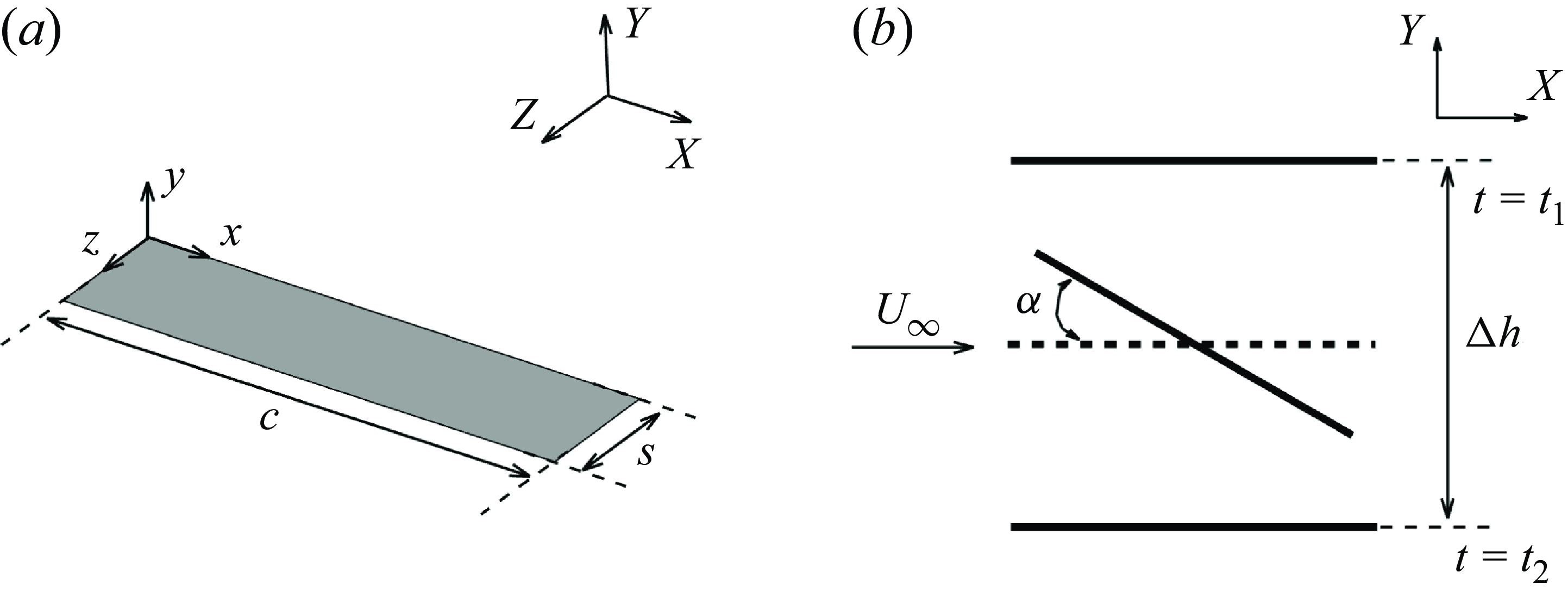
A thin flat-plate wing with a sharp leading edge is shown in figure 2(a), where the chord length and the span length are
 $c$
and
 $s$
, respectively. A practical flapping wing is simplified to this in simulations because the wing thickness and the leading-edge geometry have limited effects on the aerodynamic force and the LEV dynamics when the flow separates at the leading edge massively (Rival et al. Reference Rival, Kriegseis, Schaub, Widmann and Tropea2014; Thielicke & Stamhuis Reference Thielicke and Stamhuis2015). Coordinates
 $\textit{XYZ}$
give the orientation of the global inertial frame, and
 $xyz$
is the body-fixed coordinate frame attached to the leading edge. The spanwise direction
 $Z$
is set to be periodic to focus on the aerodynamics and LEV dynamics without the wing-tip effects. Subsequently, as shown in figure 2(b), the wing starts a one-shot heaving-down and a pitching-up motion about the centre of the chord from rest with zero angle of attack at the time
 $t_{1}$
. By time
 $t_2$
, the wing stops at the lowest point of its trajectory and returns to the zero angle of attack. This is referred to as the baseline motion in the remainder of this study. In this work, the length scale and the time scale are set to be the chord length,
 $c$
, and the convection time,
 $c/U_\infty$
, where
 $U_\infty$
is the constant free-stream velocity. Here,
 $\alpha$
is the angle of attack with respect to
 $U_\infty$
, and
 $\Delta h$
is the peak-to-peak heaving amplitude.
A flat-plate wing section: (a) top-port view of the wing section and (b) side view of the wing kinematics.

The heaving acceleration and pitching rate define the kinematics of the wing to ensure smooth heaving and pitching motion from rest. Mathematically, the baseline motion of the wing is given as follows:
 \begin{align} \ddot h_b(t) &= \begin{cases} -\Delta h_b f_b \sin (2 \pi f_b (t-t_1))H(t,a_0,t_1) H(t,-a_0,t_2), & t_1\leqslant t \leqslant t_2,\\ 0,& \text{otherwise}, \end{cases} \end{align}
 \begin{align} \dot \alpha _b(t) &= \begin{cases} \alpha _b \pi f_b \sin (2 \pi f_b (t-t_1))H(t,a_0,t_1)H(t,-a_0,t_2), & t_1\leqslant t \leqslant t_2,\\ 0,& \text{otherwise}, \end{cases} \end{align}
where
 $H$
is the smooth function at the beginning and end of the wing motion,
 $f_b$
is the dimensionless frequency of the acceleration of the baseline motion,
 $\Delta h_b$
is the dimensionless peak-to-peak heaving amplitude,
 $\alpha _b$
is the pitching amplitude of the baseline motion and
 $a_0$
is the smooth coefficient. Similar to Visbal (Reference Visbal2009),
 $H$
is defined as
 $H(t, \pm a_0, t_{1,2}) = 1 - e^{\pm a_0(t-t_{1,2})}$
. Here, the peak-to-peak heaving amplitude of the baseline motion,
 $\Delta h_b$
, is 1.0; the dimensionless frequency of the acceleration of the baseline motion,
 $f_b = 1 / (t_{2} - t_{1})$
, is 0.16; the pitching amplitude of the baseline motion,
 $\alpha _b$
, is 0.1396 radians (
 $8^\circ$
). The starting and ending times of the baseline motion,
 $t_{1}$
and
 $t_{2}$
, are set to be 1.5 and 7.75 to eliminate the start-up effects in simulations. Here,
 $t_{1}$
and
 $t_{2}$
are dimensionless, normalised by
 $c/U_\infty$
The smooth coefficient,
 $a_0$
, is 200.
For the baseline motion, the duration for the heaving-down period,
 $0.5T=1/f_b$
, is 6.25, where
 $T$
corresponds to the complete heaving-down and heaving-up cycle. Despite the one-shot motion, to aid the descriptions and discussions, the concepts of frequency and period are used. In analogy to the cyclic flapping-wing motion, the Strouhal number based on the peak-to-peak heaving amplitude,
 $St_A = ({\Delta h}/{U_\infty })( {1}/{T})$
, is 0.08, which is the upper limit of dynamic stall and the lower limit of bird flight (Baik Reference Baik2011). The maximum effective angle of attack of the baseline motion,
 $\alpha _{eff} = \alpha - \tan ^{-1}({{\rm d}h}/{{\rm d}t})$
, is approximately
 $25.60^{\circ }$
, similar to the previous studies about flapping-wing aerodynamics and the LEV dynamics (Anderson et al. Reference Anderson, Streitlien, Barrett and Triantafyllou1998; Widmann & Tropea Reference Widmann and Tropea2015; Li et al. Reference Li, Feng, Kissing, Tropea and Wang2020). Moreover, using the one-shot motion to study the LEV dynamics is reasonable as the difference in the LEV dynamics between the one-shot motion and the cyclic motion is limited (Li et al. Reference Li, Feng, Kissing, Tropea and Wang2020).
Perturbations are introduced as either the heaving-down or pitching-up motion superposed onto the baseline motion (2.1) to mimic the transverse gust and the perturbed flapping flight. The amplitude of pitching perturbations is set to be the same as the variation in
 $\alpha _{eff}$
caused by heaving perturbations. Although the moving-body method is not the same as the moving-fluid method in studying the gust (Jones et al. Reference Jones, Cetiner and Smith2022), the circulatory force variation measured in the two methods is similar (Granlund et al. Reference Granlund, Monnier, Ol and Williams2014). Mathematically, the kinematics of heaving perturbations and pitching perturbations are defined as follows:
 \begin{align} \ddot h_p(t) &= \begin{cases} -\Delta h_p \lambda ^2 f_b \sin (2 \pi \lambda f_b (t-t_{1,p}))H(t,a_0,t_{1,p}) H(t,-a_0,t_{2,p}), &\!\! t_{1,p}\leqslant t \leqslant t_{2,p},\\ 0,&\!\! \text{otherwise}, \end{cases} \end{align}
 \begin{align} \alpha _p &= \tan ^{-1}(\dot h_p + \dot h_b) - \tan^{-1}(\dot h_b), \end{align}
where
 $\Delta h_p$
is the dimensionless peak-to-peak heaving amplitude,
 $\lambda$
is the ratio between the perturbation frequency and the baseline frequency and
 $t_{1,p}$
and
 $t_{2,p}$
are the dimensionless starting and ending times of the perturbation motion. The heaving perturbation is prescribed by specifying
 $\lambda$
and
 $\Delta h_p$
. Once the heaving perturbation is determined, the pitching perturbation inducing the same variation in the effective angle of attack can be evaluated from (2.2b
). Owing to the extensive parameter space, all perturbations are synchronised at the midpoint of the baseline case in this study,
 $(t_{2} + t_{1})/2 = (t_{2,p} + t_{1,p})/2$
. To demonstrate the kinematics of the perturbed case, the heaving or pitching perturbation is superposed onto the baseline motion, as shown in figure 3. In this case,
 $\lambda$
is set to 4, and
 $\Delta h_P$
is set to be 0.125, leading to
 $T_p = 2(t_{2,p} - t_{1,p}) =3.125$
and
 $\alpha _{\textit{eff},p}=7.90^\circ$
. We study the perturbations of three different induced effective angle of attack because the effective angle of attack is considered an essential factor in studying force production of flapping wings (Hover, Haugsdal & Triantafyllou Reference Hover, Haugsdal and Triantafyllou2004), the LEV formation (Ramesh et al. Reference Ramesh, Gopalarathnam, Granlund, Ol and Edwards2014) and the gust encounter (Jones et al. Reference Jones, Cetiner and Smith2022). The parameters used in this work are summarised in table 1, which shows that the slow perturbation achieves a high
 $\alpha _{\textit{eff},p}$
with a large
 $\Delta h_p$
, and the fast perturbation achieves a high
 $\alpha _{\textit{eff},p}$
with a small
 $\Delta h_p$
.
As the Mach number for the bio-inspired flapping wings is very small, the associated flow dynamics is described by the incompressible Navier–Stokes equations
 \begin{align} \boldsymbol{\nabla }\boldsymbol{\cdot }\boldsymbol{u} &= 0 , \end{align}
 \begin{align} \frac {\partial \boldsymbol{u}}{\partial t} + \boldsymbol{ u} \boldsymbol{\cdot }\boldsymbol{\nabla }\boldsymbol{ u} &= -\boldsymbol{\nabla }p + \frac {1}{{\textit{Re}}} {\nabla} ^2 \boldsymbol{u}+ \boldsymbol{ f}, \end{align}
where
 $p$
is the dimensionless pressure,
 $\boldsymbol{u}$
is the dimensionless velocity,
 $\boldsymbol{f}$
is the dimensionless body force density and
 ${\textit{Re}}$
is the Reynolds number defined as
 ${\textit{Re}} = U_\infty c / \nu$
, with
 $\nu$
being the kinematic viscosity of the fluid.
A comparison of wing motions between the baseline case and the perturbed cases of
 $\alpha _{\textit{eff},p}=7.90^\circ$
and
 $\lambda=2$
, 4 and 8. (a) The heaving displacement, (b) the pitching amplitude and (c) the effective angle of attack.

2.2. Numerical methods
The recursive regularised lattice Boltzmann method (LBM) with a diffusive immersed boundary method (IBM) is utilised to solve the flow dynamics due to its simplicity, efficiency and intrinsic parallel nature (Chen & Doolen Reference Chen and Doolen1998; Aidun & Clausen Reference Aidun and Clausen2010; Krüger et al. Reference Krüger, Kusumaatmaja, Kuzmin, Shardt, Silva and Viggen2017). The details of this method have been well documented in our previous works (Xu et al. Reference Xu, Tian, Young and Lai2018; Jin et al. Reference Jin, Wang, Ravi, Young, Lai and Tian2024; Wang et al. Reference Wang, Liu, Jin, Huang, Young and Tian2024a ). Here, only a brief description is given. The LBM solves the discrete lattice Boltzmann equation
 \begin{equation} f_i( \boldsymbol{x}+\boldsymbol{e}_i \Delta t,t+\Delta t) - f_i( \boldsymbol{x},t) = \varOmega _i( \boldsymbol{x},t) + \Delta t G_i, \end{equation}
where
 $f_i$
is the particle distribution function,
 $\boldsymbol{e_{i}}$
is the discrete lattice velocity,
 $\varOmega _i( \boldsymbol{x},t)$
is the collision function,
 $\Delta t$
is the time step and
 $G_i$
is the discrete source term due to the body force. The force scheme proposed by Guo, Zheng & Shi (Reference Guo, Zheng and Shi2002a
) and the recursive regularised model presented by Coreixas et al. (Reference Coreixas, Wissocq, Puigt, Boussuge and Sagaut2017) are used to determine
 $G_i$
and
 $\varOmega _i$
, according to
 \begin{align} G_i&=\Big (1-\frac {1}{2\tau }\Big )\omega _i\Big (\frac {\boldsymbol{e}_i-\boldsymbol{u}}{c_s^2} + \frac {\boldsymbol{e}_i \boldsymbol{\cdot }\boldsymbol{u}}{c_s^4}\boldsymbol{e}_i\Big ) \boldsymbol{\cdot }\boldsymbol{f}, \end{align}
 \begin{align} &\qquad\qquad\quad \varOmega _i(\boldsymbol{x},t) = \frac {1}{\tau }f_i^{(1)}, \end{align}
The perturbation amplitude
 $\Delta h_p$
at different
 $\alpha _{\textit{eff},p}$
and different
 $\lambda$
.

where
 $\tau$
is the dimensionless relaxation time defined as
 $\tau = \nu / (c_s^2 \Delta t) + 1/2$
,
 $f_i^{(1)}$
is the non-equilibrium part of the particle distribution function
 $f_i$
from the recursive regularised procedure (Latt & Chopard Reference Latt and Chopard2006; Coreixas et al. Reference Coreixas, Wissocq, Puigt, Boussuge and Sagaut2017),
 $c_s$
is the ideal sound speed in the LBM model defined by
 $c_s = \Delta x / (\Delta t \sqrt {3})$
,
 $\omega _i$
is the weighted parameter and
 $\Delta x$
is the grid size. The 3-D nineteen discrete velocity (D3Q19) lattice model is used in this work. To avoid duplication and verbosity, the equations for evaluating the equilibrium part and the non-equilibrium part of the particle distribution function,
 $f_i^{(eq)}$
, and
 $f^{(1)}_i$
in the recursive regularised collision model can be found in Coreixas et al. (Reference Coreixas, Wissocq, Puigt, Boussuge and Sagaut2017). The fluid density, pressure and velocity can be evaluated from
 $f_i$
according to the following equations:
 \begin{eqnarray} \rho =\sum _{i}f_i,\quad p=\rho c_s^2, \quad \mathrm{and} \quad \boldsymbol{u}=\left (\sum _{i}\boldsymbol{e}_i f_i+\frac {1}{2}\boldsymbol{f}\Delta t\right ) \Bigg /\rho . \end{eqnarray}
The boundary condition of the wing is achieved by the feedback IBM due to its simplicity in handling boundary conditions at the fluid–structure interface involving a complex geometry and large movement (Goldstein, Handler & Sirovich Reference Goldstein, Handler and Sirovich1993; Mittal & Iaccarino Reference Mittal and Iaccarino2005; Huang & Tian Reference Huang and Tian2019; Griffith & Patankar Reference Griffith and Patankar2020). Specifically, a body force is applied near the solid boundary to achieve the no-slip boundary condition
 \begin{equation} \boldsymbol{f} = -\int \boldsymbol{F}(\boldsymbol{s},t)\delta ( \boldsymbol{x}-\boldsymbol{X}(\boldsymbol{s},t)){\rm d}A, \end{equation}
where
 $\boldsymbol{F}(\boldsymbol{s},t)$
is the Lagrangian force on the structure,
 ${\rm d}A$
is the surface area of the structure element and
 $\delta$
is the Dirac delta function. Also,
 $\boldsymbol{X}(\boldsymbol{s},t)$
is the position of the structure element at time
 $t$
, and
 $\boldsymbol{s}$
represents the curvilinear coordinates attached to the structure element. The value of
 $\boldsymbol{F}(\boldsymbol{s},t)$
is evaluated by the feedback scheme
 \begin{align} \boldsymbol{F} &= \beta (\boldsymbol{U}_{ib} (\boldsymbol{s},t) - \boldsymbol{U}(\boldsymbol{s},t)), \end{align}
 \begin{align} \boldsymbol{U}_{ib}(\boldsymbol{s},t) &= \int \boldsymbol{u}(\boldsymbol{x},t) \delta ( \boldsymbol{x}-\boldsymbol{X}(\boldsymbol{s},t)){\rm d}\boldsymbol{x}, \end{align}
where
 $\beta$
is the feedback coefficient,
 $\boldsymbol{U}_{ib}(\boldsymbol{s},t)$
is the fluid velocity on the structure element interpolated from the surrounding fluid and
 $\boldsymbol{U}(\boldsymbol{s},t)$
is the moving velocity of the structure element. In this work, the feedback coefficient
 $\beta$
is set to be 2.6 in the LBM unit, as suggested by Huang et al. (Reference Huang, Liu, Wang, Ravi, Young, Lai and Tian2022). In the simulations, the Dirac delta function
 $\delta (\boldsymbol{x})$
is replaced by the smoothed Dirac delta function
 $\delta _h (\boldsymbol{x})$
proposed by Peskin (Reference Peskin2002). For the simulations at
 ${\textit{Re}}=2$
0 000, the four-point smoothed Dirac delta function proposed by Yang et al. (Reference Yang, Zhang, Li and He2009) is used due to the better numerical stability. At
 ${\textit{Re}}=2$
0 000, the turbulent flow is modelled using the large eddy simulation where (2.3) can be considered as the filtered Navier–Stoke equations. Turbulence modelling is implemented by adding the subgrid-scale eddy viscosity
 $\nu _{\textit{sgs}}$
to the kinematic viscosity. The final effective dimensionless relaxation time is evaluated as follows (Malaspinas & Sagaut Reference Malaspinas and Sagaut2012):
 \begin{equation} \tau _{eff} = \frac {\nu + \nu _{\textit{sgs}}}{{c_s}^2 \Delta t} + \frac {1}{2}. \end{equation}
The shear-improved Smagorinsky model (Lévêque et al. Reference Lévêque, Toschi, Shao and Bertoglio2007) is used due to the existence of the homogeneous direction (
 $Z$
) in the simulations. The accuracy of the model is comparable to that of the dynamic Smagorinsky model but with a much lower computational expense. In the model, the subgrid-scale eddy viscosity is evaluated by
 \begin{equation} \nu _{\textit{sgs}} = (C \Delta x)^2 ( | {\boldsymbol{S}} | - | \langle {\boldsymbol{S}} \rangle |), \end{equation}
where
 $| {\boldsymbol{S}} |$
is the magnitude of the instantaneous strain rate tensor calculated by the second-order central difference scheme,
 $| \langle {\boldsymbol{S}} \rangle |$
is the magnitude of the spatial average strain rate tensor along the
 $Z$
-direction at every time step and
 $C=0.12$
is the Smagorinsky constant.
2.3. Simulation set-up
Multiblock mesh refinement (Filippova & Hänel Reference Filippova and Hänel2000; Yu, Mei & Shyy Reference Yu, Mei and Shyy2002; Xu et al. Reference Xu, Tian, Young and Lai2018) is used to increase the computational efficiency as well as the accuracy, where the block with a finer mesh is applied near the wing covering the moving trajectory, and coarser blocks with a coarsening ratio of 2 are applied in the far field. The whole computational domain is a rectangular box spanning from
 $(-15c, -15c, 0)$
to
 $(30c, 15c, s)$
. The periodic boundary condition is applied in the spanwise direction. In the simulations,
 $s=0.2c$
for
 ${\textit{Re}}=2000$
and
 $0.4c$
for
 ${\textit{Re}}=2$
0 000 are adopted. Here,
 $s=0.2c$
is sufficient for simulations at
 ${\textit{Re}}=2000$
because the flow is considered laminar, and the flow structures remain two-dimensional. At
 ${\textit{Re}}=2$
0 000, the computational domain in the spanwise direction needs to be large enough to resolve the flow structures of the largest spanwise wavelength. The effects of the spanwise length on the aerodynamic force and the LEV dynamics at
 ${\textit{Re}}=2$
0 000 are presented in Appendix A, showing that
 $s = 0.4c$
is enough. The Dirichlet-type velocity boundary condition,
 $\boldsymbol{u} = (U_\infty ,0,0)$
, and zero gradient pressure boundary condition are used for physical boundaries except for the outlet surface, where the Dirichlet-type pressure boundary condition,
 $p=p_0$
, and zero gradient velocity boundary condition are applied. The non-equilibrium extrapolation method evaluates
 $f_i$
at the boundary lattices (Guo et al. Reference Guo, Zheng and Shi2002b
). The absorbing layers (Xu & Sagaut Reference Xu and Sagaut2013) are applied at the lattices near the physical boundaries to minimise the reflections due to acoustic waves, where the thickness of the absorbing layer is
 $10c$
near the outlet, and
 $5c$
near other external boundaries. The whole computational domain is initialised with
 $\boldsymbol{u}=(U_\infty ,0,0)$
and
 $\rho = \rho _0$
. The in-house solver used in this work has been validated and utilised in our previous work (Jin et al. Reference Jin, Wang, Ravi, Young, Lai and Tian2024). A mesh independence study is conducted to ensure that the results reported here are independent of the mesh spacing, as shown in Appendix A.
The lift, drag and moment coefficients of the wing for describing the aerodynamic performance are defined as follows:
 \begin{equation} C_L =\frac {L}{\frac {1}{2} \rho U_\infty ^2 A} , \quad C_D =\frac {D}{\frac {1}{2} \rho U_\infty ^2 A}, \quad C_M =\frac {M}{\frac {1}{2} \rho U_\infty ^2 A c}, \end{equation}
where
 $L$
is the lift on the wing,
 $D$
is the drag on the wing and
 $M$
is the pitching moment about the pivot point.
3. Results and discussion
3.1. Overview of the lift variations at
 ${{\textit{Re}}}=2000$
and
${\textit{Re}}=20\,000$


The lift variations under heaving perturbations and pitching perturbations at both
 ${\textit{Re}}=2000$
and
 ${\textit{Re}}=2$
0 000 are first analysed to reveal the overall effects of the perturbations. The time histories of
 $C_L$
encountering slow, medium and fast perturbations (
 $\lambda=2$
, 4 and 8) at
 ${\textit{Re}}=2000$
and 20 000 are shown in figures 4 and 5, respectively. Animations showing the evolution of vortices are provided in the supplementary movies. The lines with markers are the lift component of the added mass force of a thin flat-plate wing evaluated from the potential flow theory (Leishman Reference Leishman2002; Corkery Reference Corkery2019),
 $C_{L,add} = - \rho ({\pi }/{4}) bc \dot U_n / (1/2 bc \rho U_\infty ^2) \cos {\alpha }$
, where
 $U_n$
is the wing-normal component of the acceleration of the centroid. The two vertical dashed lines refer to the starting and ending times of perturbations. Increasing
 $\lambda$
or
 $\alpha _{\textit{eff},p}$
of the perturbations, the peaks of
 $C_L$
during the perturbation increase similarly at both
 ${\textit{Re}}=2000$
and 20 000. This observation is similar to the work of Bhat et al. (Reference Bhat, Mazharmanesh, Medina, Tian, Young, Lai and Ravi2023), which considered the pitching perturbation effects on a revolving wing at low
 ${\textit{Re}}$
. Overall, the lift increase during heaving perturbations is larger than pitching perturbations when they have the same
 $\alpha _{\textit{eff},p}$
. Moreover, it can be seen that lift variations due to perturbations are not sensitive to
 ${\textit{Re}}$
, especially during the perturbation period, where the time histories of
 $C_L$
vary similarly. Perturbations dominate lift variations instead of
 ${\textit{Re}}$
because the viscous time scale,
 $c^2/\nu$
, is much larger than the acceleration time scale here,
 $(c/a)^{1/2}$
, where
 $a$
is the magnitude of the wing acceleration. This is also confirmed in our additional numerical tests on cases at
 ${\textit{Re}}=2$
00, 5000 and 10 000, in which
 $C_L$
varies similarly during the perturbation period.
The variations in
 $C_L$
encountering the heaving and pitching perturbations for
 $\lambda=2$
, 4 and 8 at
 ${\textit{Re}}=2000$
. Panels (a), (c) and (e) are for the heaving perturbations. Panels (b), (d) and ( f) are for the pitching perturbations. Lines with markers are the estimated added mass force in the vertical direction. The two vertical dash lines refer to the starting and ending times of perturbations.

The variations in
 $C_L$
encountering the heaving and pitching perturbations for
 $\lambda=2$
, 4 and 8 at
 ${\textit{Re}}=2$
0 000. Panels (a), (c) and (e) are for the heaving perturbations. Panels (b), (d) and ( f) are for the pitching perturbations. Lines with markers are the estimated added mass force in the vertical direction. The two vertical dash lines refer to the starting and ending times of perturbations.

Regarding perturbations of
 $\lambda=2$
, the added mass forces are pretty small for both heaving perturbations and pitching perturbations, as shown in figures 4(a), 4(b), 5(a) and 5(b). Increasing
 $\alpha _{\textit{eff},p}$
from
 $3.95^\circ$
to
 $15.80^\circ$
, the peak of
 $C_L$
during the perturbation increases, but the increase in the added mass force is still relatively small. This suggests that the increase in the circulatory force dominates the overall increase in
 $C_L$
at
 $\lambda=2$
. Regarding pitching perturbations of
 $\lambda=2$
, as shown in figures 4(b) and 5(b), the time when
 $C_L$
reaches its maximum value is earlier than the heaving perturbation (figures 4
a and 5
a). This is because the phase of
 $\dot \alpha$
is in advance of the phase of
 $\alpha$
. When perturbation encounters are over,
 $C_L$
quickly recovers to the baseline cases at
 ${\textit{Re}}=2000$
, regardless of
 $\alpha _{\textit{eff},p}$
and the perturbation type. However, relatively large deviations from the baseline case are observed at
 ${\textit{Re}}=2$
0 000.
When the perturbation duration becomes shorter, increasing
 $\lambda$
from 2 to 4, the added mass effects become more prominent due to the more significant wing acceleration. The phase difference between the total
 $C_L$
and the added mass force reduces, suggesting that the added mass forces start to dominate the overall lift variation. For heaving perturbations, the negative peaks in
 $C_L$
near the end of the perturbation become more pronounced, as shown in figures 4(c) and 5(c). Regarding pitching perturbations, there is just one apparent positive peak in
 $C_L$
during the perturbation, as shown in figures 4(d) and 5(d). For
 $\lambda = 4$
cases at
 ${\textit{Re}}=2000$
, the time histories of
 $C_L$
after perturbations deviate more from the baseline case than the cases of
 $\lambda=2$
. However, at
 ${\textit{Re}}=2$
0 000, this difference is not observed, where the time histories of
 $C_L$
do not differentiate significantly from the baseline case for both heaving perturbations and pitching perturbations after the perturbation period. This suggests perturbations have a notable impact on the vortex evolution around the wing at
 ${\textit{Re}}=2000$
.
Further shortening perturbations to
 $\lambda = 8$
, results in the added mass effects being more significant, as shown in figures 4(e), 4( f), 5(e) and 5( f). The added mass effects dominate the lift increment now. In terms of effects on
 $C_L$
after the perturbation,
 $C_L$
is more likely to be affected by pitching perturbations at
 ${\textit{Re}}=2000$
, comparing figures 4(e) and 4( f). However, for the perturbations at
 ${\textit{Re}}=2$
0 000,
 $C_L$
quickly recovers to the baseline case except for the largest pitching perturbation with
 $\alpha _{\textit{eff},p} = 15.80^\circ$
.
3.2. Lift increment scaling and the LEV dynamics at
${\textit{Re}}=2000$

We analyse the
 $C_L$
increment and the LEV evolution to uncover the flow physics during perturbations in this section. Without loss of generality, we only analyse the lift increment (
 $\Delta C_L$
) at
 ${\textit{Re}}=2000$
because the time histories of
 $C_L$
at
 ${\textit{Re}}=2000$
and 20 000 are similar, particularly during perturbations (see figures 4 and 5). To investigate the relationship between
 $\Delta C_L$
and the perturbation size,
 $\alpha _{\textit{eff},p}$
, the time histories of
 $\Delta C_L$
during perturbations are normalised by
 $\alpha _{\textit{eff},p}$
.
3.2.1. Heaving perturbations at
${\textit{Re}} = 2000$

The effects of heaving perturbations are analysed first in this sub-section, and the effects of pitching perturbations will be discussed in the ensuing sub-section. It can be seen that
 $\Delta C_L$
is scaled with
 $\alpha _{\textit{eff},p}$
in figure 6, in which it varies similarly despite some small difference. This implies that the increase in the perturbation size,
 $\alpha _{\textit{eff},p}$
, affects the vortex dynamics similarly during heaving perturbations.
Value of
 $\alpha _{\textit{eff},p}$
scaled
 $\Delta C_L$
for slow, medium and fast heaving perturbations at
 ${\textit{Re}}=2000$
.

Spanwise vorticity
 $\omega _z$
contour superposed by the streamlines of heaving perturbations for
 $\lambda=2$
at
 ${\textit{Re}}=2000$
.

The evolution of the circulation of the primary LEV under heaving perturbations for
 $\lambda=2$
at
 ${\textit{Re}}=2000$
. Small insets are snapshots showing the identified LEV boundaries from the vortex identification method. The two vertical dashed lines indicate the duration of the perturbation.

The flow contours of the baseline case are given in Appendix B for comparison. Figure 7 shows the effects of heaving perturbations at
 $\lambda = 2$
on the flow field, while figure 8 displays the time history of the primary LEV circulation. Here, the method proposed by Graftieaux, Michard & Grosjean (Reference Graftieaux, Michard and Grosjean2001) is used to identify the boundary of the LEV, and the circulation of the LEV is computed by integrating the vorticity in this boundary. The snapshots of the vorticity contour with the identified LEV boundary presented in the wing reference frame are inserted into the figure to help explain the variations in
 $\varGamma$
. It is noted that the peaks in figure 8 between
 $t=$
3.5 and 4.0 are due to the disconnection of the leading-edge shear layer and the primary LEV, where the LEV and the shear layer are identified as one part when the nascent LEV is still small, as shown in the insets in figure 8. Overall, the heaving perturbations of
 $\lambda = 2$
do not trigger the vorticity layer eruption, in which the bluff-body detachment mechanism still dominates the LEVs’ detachment for all three cases shown in figures 7 and 8. From figure 8, it can be observed that the LEV circulation in the cases subjected to the heaving perturbations of
 $\alpha _{\textit{eff},p}= 3.95^{\circ }$
,
 $7.90^{\circ }$
and
 $15.80^{\circ }$
no longer increases after
 $t=$
6.0, 5.8 and 5.4, respectively. Specifically, the reattachment points of the LEVs (defined in figure 1) are observed to arrive and exceed the trailing edge at
 $t=$
5.4 for these three cases at
 $\lambda = 2$
, as shown by the streamlines in figure 7. Thus, the growth of LEVs is restricted by the wing’s chord length, as in the baseline case. Consequently, the lift increments scaled by
 $\alpha _{\textit{eff},p}$
in figure 6(a) collapse onto each other with a minor difference. Moreover, a larger perturbation creates a larger distance between the wing and the LEV, as shown in figure 7. For example, we found the distance between the wing and the LEV increases 15.8 %, 33.3 % and 65.4 % on increasing
 $\alpha _{\textit{eff},p}$
from
 $\alpha _{\textit{eff},p}= 3.95^{\circ }$
to
 $15.80^{\circ }$
compared with the baseline case (0.240
 $c$
) at
 $t=$
5.4. And similarly, the circulation increases by 14.5 %, 27.3 % and 48.0 % compared with the baseline case (1.54), as shown in figure 8.
Either increased circulation or decreased vortex–wall distance generally indicates a stronger vortex–wall interaction, resulting in a more dramatic viscous response in the surface flow (Doligalski et al. Reference Doligalski, Smith and Walker1994). The increased heaving perturbation at
 $\lambda = 2$
tends to decrease the intensity of the vortex–wall interaction, as the increase in the LEV circulation is smaller than the increase in the vortex–wall distance. Therefore, increasing the perturbation size at
 $\lambda = 2$
does not lead to the eruption-type LEV detachment, caused by the stronger vortex–wall interaction, but rather a bluff-body LEV detachment.
Spanwise vorticity
 $\omega _z$
contour superposed by the streamlines of heaving perturbations for
 $\lambda=4$
at
 ${\textit{Re}}=2000$
. The contour legend as per figure 7.

The evolution of the circulation of the primary LEV under heaving perturbations for
 $\lambda=4$
at
 ${\textit{Re}}=2000$
. All the insets correspond to the
 $\alpha _{\textit{eff},p} = 15.80^{\circ }$
case. Legend and captions as per figure 8.

For heaving perturbations of
 $\lambda=4$
, shown in figures 9 and 10, the effects of perturbations on vortices are similar to those of
 $\lambda=2$
. Heaving perturbations of
 $\lambda=4$
do not trigger the vorticity eruption. As shown in figure 10, the LEV circulation no longer increases after
 $t$
around 5.8, 5.7 and 5.4 with increasing
 $\alpha _{\textit{eff},p}$
, which is slightly earlier than those observed for
 $\lambda = 2$
. From figure 9 by carefully comparing the position of the LEV reattachment point with the trailing edge of the chord, it can be seen that the LEV reattachment points have just passed the trailing edge for
 $\alpha _{\textit{eff},p}=$
 $3.95^{\circ }$
and
 $7.90^{\circ }$
at
 $t=$
5.7. For
 $\alpha _{\textit{eff},p}=$
 $15.80^{\circ }$
, the LEV reattachment point arrived at the trailing edge at
 $t=$
5.4 and passed the trailing edge at
 $t=$
5.7. Therefore, the LEV growth under heaving perturbations of
 $\lambda = 4$
is still governed by the chord length of the wing, as in the baseline cases and the cases subject to heaving perturbations of
 $\lambda = 2$
. The increase in the LEV–wall distance and the LEV circulation can also be determined from figures 9 and 10. Specifically, the increases in the LEV–wall distance are 10.0 %, 17.1 % and 41.7 % compared with the baseline case at
 $t=$
5.4. Additionally, the increases in LEV circulation at
 $t=$
5.4 are 12.1 %, 23.35 % and 44.36 %, respectively. Different to the heaving perturbations of
 $\lambda = 2$
, the increase in the LEV circulation is larger than the increase in the LEV–wall distance, which indicates that the heaving perturbations of
 $\lambda = 4$
increase the viscous response in the surface flow, but still not sufficiently to cause the vorticity eruption. Thus, as increasing
 $\alpha _{\textit{eff},p}$
of the perturbations at
 $\lambda = 4$
does not change the dominant LEV detachment mechanism, the lift increment scales well with
 $\alpha _{\textit{eff},p}$
, as shown in figure 6(b).
Spanwise vorticity
 $\omega _z$
contour superposed by the streamlines of heaving perturbations for
 $\lambda=8$
at
 ${\textit{Re}}=2000$
. The contour legend as per figure 7. A and B: entrainment of the erupted vorticity layer into the LEV; C: vorticity eruption.

The evolution of the circulation of the primary LEV under heaving perturbations for
 $\lambda=8$
at
 ${\textit{Re}}=2000$
. All the insets correspond to the
 $\alpha _{\textit{eff},p} = 7.90^{\circ }$
case. Legend and captions as per figure 8.

For vorticity contours and circulation variations of heaving perturbations at
 $\lambda=8$
, as shown in figures 11 and 12, significant changes in the LEV evolution are observed. All three perturbations change the LEV detachment mechanism from chord-length dominated to vorticity-eruption dominated. Specifically, as shown in figure 12, the LEV circulation stops growing after
 $t=$
5.1, 5.0 and 4.8 for
 $\alpha _{\textit{eff},p}=$
 $3.95^{\circ }$
,
 $7.90^{\circ }$
and
 $15.80^{\circ }$
, respectively. In addition, large, sharp peaks at
 $t \approx 4.8$
for
 $\alpha _{\textit{eff},p}=$
 $7.90^{\circ }$
and
 $15.80^{\circ }$
and a smaller peak at
 $t \approx 5$
for
 $\alpha _{\textit{eff},p}=$
 $3.95^{\circ }$
contrast with the smooth increase in circulation for the previous two cases (
 $\lambda = 2, 4$
). The vorticity eruption can be observed for
 $\alpha _{\textit{eff},p}=$
 $15.80^{\circ }$
at
 $t=4$
.9, indicated by label C in figure 11. For
 $\alpha _{\textit{eff},p}=$
 $3.95^{\circ }$
and
 $7.90^{\circ }$
, the vorticity eruption occurs later than that of
 $\alpha _{\textit{eff},p}=$
 $15.80^{\circ }$
. In each of these cases, the LEV has not passed the trailing edge of the chord when detachment occurs (by observing positions of the LEV reattachment point with respect to the trailing edge at detachment time). Moreover, it can be seen that the ejected positive vorticity begins to wrap around the LEV at
 $t=$
5.4, indicated by labels A and B. In summary, for all three heaving perturbations at
 $\lambda=8$
, the LEV detachment mechanism is the vorticity layer eruption, in contrast to the
 $\lambda = 2$
and 4 cases, which are both bluff-body detachment. Since for
 $\lambda = 8$
all three cases are triggered by the same detachment mechanism (vorticity eruption), the lift increment for them scales similarly with the increase in
 $\alpha _{\textit{eff},p}$
, as shown in figure 6(c). It can be seen that, despite the same
 $\alpha _{\textit{eff},p}$
for slow and fast heaving perturbations, the vorticity layer eruption is more likely to occur subject to the fast heaving perturbations.
Time histories of
 $C_M$
under heaving perturbations at
 ${\textit{Re}}=2000$
. Panels show (a)
 $\lambda=2$
, (b)
 $\lambda=4$
and (c)
 $\lambda=8$
.

The time histories of the pitching moment coefficient about the mid-chord position (pivot point) are shown in figure 13. Under the slow and medium perturbations, as shown in figures 13(a) and 13(b), the negative peaks of
 $C_M$
, corresponding to the occurrence of the trailing-edge stall, are not significantly affected by the perturbation. Here, the LEV travels downstream along the wing surface and then induces the formation of the trailing-edge vortex (TEV). For
 $\lambda=8$
, as shown in figure 13(c), the heaving perturbations affect
 $C_M$
significantly. There are two reasons for this. Firstly, the vorticity layer eruption caused by the fast perturbation advects the primary LEV away from the wing in the wing-normal direction due to the interaction between the LEV and the vorticity ejected from the boundary layer. The larger vertical distance between the primary LEV and the wing surface reduces the suction effects from the primary LEV as it approaches the trailing edge, leading to reduced strength of the newly formed TEV. Secondly, due to the early detachment of the primary LEV, the newly formed LEV exerts a positive pitching moment on the wing, as shown in the snapshot at
 $t=6.0$
of figure 11. Therefore, the negative peak of
 $C_M$
for the wing encountering the heaving perturbation of
 $\lambda = 8$
is reduced.
3.2.2. Pitching perturbations at
${\textit{Re}} = 2000$

Value of
 $\alpha _{\textit{eff},p}$
scaled
 $\Delta C_L$
for slow, medium and fast pitching perturbations at
 ${\textit{Re}}=2000$
.

For the pitching perturbations, there are relatively large differences in
 $\Delta C_L / \alpha _{\textit{eff},p}$
compared with the heaving perturbations, as shown in figure 14. This indicates that increasing
 $\alpha _{\textit{eff},p}$
of the pitching perturbation affects the LEV evolution differently.
Spanwise vorticity
 $\omega _z$
contour superposed by the streamlines of pitching perturbations for
 $\lambda=2$
at
 ${\textit{Re}}=2000$
. The contour legend as per figure 7.

The evolution of the circulation of the primary LEV under pitching perturbations for
 $\lambda=2$
at
 ${\textit{Re}}=2000$
. Legend and captions as per figure 8.

Consider the vorticity contours superposed by the streamlines (figure 15) and the time history of the LEV circulation (figure 16) under the pitching perturbations of
 $\lambda=2$
. Compared with figures 7 and 8, the effects of pitching perturbations are similar to those of heaving perturbations at
 $\lambda = 2$
. This indicates that the flow contours are primarily affected by the variations in
 $\alpha _{\textit{eff},p}$
when the perturbations are slow, regardless of pitching or heaving, despite the different time history of the force. Overall, the LEV detachment mechanism is bluff-body dominated, in which the growth of the LEV is limited by the chord length of the wing, as in the baseline case and the cases subject to heaving perturbations of
 $\lambda=2$
. Specifically, it can be seen that the LEV circulation, which is smooth throughout after
 $t = 4$
for all three cases, keeps increasing until its reattachment point reaches the trailing edge, as shown in figures 15 and 16. Due to the similar flow contours and the same LEV detachment mechanism among
 $\alpha _{\textit{eff},p}=$
 $3.95^{\circ }$
,
 $7.90^{\circ }$
and
 $15.80^{\circ }$
, the variations in
 $\Delta C_L$
scale with
 $\alpha _{\textit{eff},p}$
(figure 14
a).
Spanwise vorticity
 $\omega _z$
contour of the pitching perturbation for
 $\lambda=4$
and
 ${\textit{Re}}=2000$
. The contour legend as per figure 7.

The evolution of the circulation of the primary LEV under pitching perturbations for
 $\lambda=4$
at
 ${\textit{Re}}=2000$
. All the insets correspond to the
 $\alpha _{\textit{eff},p} = 15.80^{\circ }$
case. Legend and captions as per figure 8.

Consider the vorticity contours (figure 17) and the LEV circulation (figure 18) under pitching perturbations at
 $\lambda=4$
. At
 $\alpha _{\textit{eff},p} = 3.95^{\circ }$
, the growth of the LEV is similar to the baseline, whereby the LEV detaches due to the chord length of the wing. As
 $\alpha _{\textit{eff},p}$
increases, the LEV evolution varies significantly, in which the LEVs’ detachment mechanism now becomes the vorticity layer eruption dominated. It can be seen the circulation (figure 18) for
 $\alpha _{\textit{eff},p}=$
 $7.90^{\circ }$
and
 $15.80^{\circ }$
both show non-smooth behaviour with relatively sharp peaks, whereas the circulation for
 $\alpha _{\textit{eff},p}=$
 $3.85^{\circ }$
is much smoother without a sharp peak. In detail, the circulation of the primary LEV stops growing after
 $t=$
5.7 and 5.2 for
 $\alpha _{\textit{eff},p}=$
 $3.95^{\circ }$
and
 $7.90^{\circ }$
, as shown in figure 18. The reattachment point of the LEV arrives at the trailing edge at
 $t=$
5.7 for
 $\alpha _{\textit{eff},p}=$
 $3.95^{\circ }$
(figure 17). And, for
 $\alpha _{\textit{eff},p}=$
 $7.90^{\circ }$
, it just passes the trailing edge by a small amount at
 $t=$
5.7. Therefore, the detachment of the LEV for
 $\alpha _{\textit{eff},p}=$
 $3.95^{\circ }$
and
 $\alpha _{\textit{eff},p}=$
 $7.90^{\circ }$
is classified into bluff-body dominated and vorticity layer eruption dominated, respectively. Regarding
 $\alpha _{\textit{eff},p}=$
 $15.80^{\circ }$
, the vorticity layer eruption can be observed at
 $t=$
5.1 and 5.7 in figure 17, in which a thin spire of fluid containing positive vorticity is ejected from the surface flow due to the strong LEV–wall interaction. It is noted that the LEV detachment mechanism for
 $\alpha _{\textit{eff},p}=$
 $7.90^{\circ }$
is more like a mixture of bluff-body shedding and vorticity layer eruption. The eruption is not as strong as the one observed in
 $\alpha _{\textit{eff},p}=$
 $15.80^{\circ }$
, and the vorticity contours do not differentiate significantly from those of
 $\alpha _{\textit{eff},p}=$
 $3.95^{\circ }$
before
 $t=$
5.7. Thus, the lift increment scaled by
 $\alpha _{\textit{eff},p}$
are similar between
 $\alpha _{\textit{eff},p}=$
 $3.95^{\circ }$
and
 $\alpha _{\textit{eff},p}=$
 $7.90^{\circ }$
(figure 14
b). And, a relatively large difference is observed for
 $\alpha _{\textit{eff},p}=$
 $15.80^{\circ }$
.
Spanwise vorticity
 $\omega _z$
contour of the pitching perturbation for
 $\lambda=8$
and
 ${\textit{Re}}=2000$
. The contour legend as per figure 7.

The evolution of the circulation of the primary LEV under pitching perturbations for
 $\lambda=8$
at
 ${\textit{Re}}=2000$
. All the insets correspond to
 $\alpha _{\textit{eff},p} = 15.80^{\circ }$
case. Legend and captions as per figure 8.

Finally we turn to the vorticity contours (figure 19) and the LEV circulation (figure 20) under pitching perturbations at
 $\lambda=8$
. Here, the LEV’s detachment mechanism is much more clear-cut compared with
 $\lambda=4$
. For all three cases of
 $\lambda=8$
, the detachment mechanism is vorticity layer eruption. Specifically, the circulation of the primary LEV no longer increases after
 $t$
around 4.8, as shown in figure 20. The abrupt increase following the drop between
 $t=4$
.8 and 5.0 is caused by the merging of the primary LEV with the second LEV, as shown in the insets of figure 20. The corresponding vorticity layer eruption and the vortex merging are also shown in the snapshots at
 $t=4$
.8 and 5.0 of figure 19. After the merge of the two LEVs, a second time vorticity layer eruption is observed at
 $t=$
5.5. Then, the newly formed LEV from vortex merging detaches from the wing, and the third LEV forms at
 $t=$
5.8. On the whole, for all the pitching perturbations at
 $\lambda=8$
, the dominant LEV detachment mechanism is vorticity layer eruption, and it affects the vortex dynamics similarly. Therefore, the lift increment scales well with the increase in
 $\alpha _{\textit{eff},p}$
except for the period near the end of the perturbations,
 $t = 4.8 \sim 5.0$
(figure 14
c).
Time histories of
 $C_M$
under pitching perturbations at
 ${\textit{Re}}=2000$
. Panels show (a)
 $\lambda=2$
, (b)
 $\lambda=4$
and (c)
 $\lambda=8$
.

The observations on the LEV dynamics under pitching perturbations discussed above are consistent with the variations in
 $C_M$
, as shown in figure 21. For
 $\lambda=2$
, the effects of perturbations on
 $C_M$
are small (figure 21
a), where the LEV dynamics remains almost the same as that of the baseline case. The LEV detachment is governed by the chord length of the wing. For
 $\lambda=4$
, the detachment of the LEV is still governed by the chord length of the wing at
 $\alpha _{\textit{eff},p} = 3.95^\circ$
. As
 $\alpha _{\textit{eff},p}$
increases, the vorticity layer eruption happens, as shown in figure 17. Although the dominant LEV detachment mechanism is vorticity layer eruption for
 $\alpha _{\textit{eff},p} = 7.90^\circ$
, the eruption is not as strong as the one observed in
 $\alpha _{\textit{eff},p} = 15.80^\circ$
. Its influence on the following formation of the TEV is not large. Therefore, the trailing-edge stall is only absent in the case of
 $\alpha _{\textit{eff},p} = 15.80^\circ$
, as shown in figure 21(b). When
 $\lambda$
increases to 8, all the perturbations cause the early detachment of the LEV due to the strong vorticity layer eruption, where the formations of the TEV are weaker than those whose LEV detachment is governed by the chord length of the wing. Therefore, the negative peak in
 $C_M$
disappears for all three
 $\alpha _{\textit{eff},p}$
values (figure 21
c).
Overall, it can be seen that the fast pitching perturbations induce a stronger vortex–wall interaction, resulting in vorticity layer eruption. This is consistent with the observations in heaving perturbations. Compared with heaving perturbations, pitching perturbations are more likely to cause the vorticity layer eruption, as shown in the results of pitching and heaving perturbations for
 $\lambda = 4$
. In terms of accuracy of the scaling in
 $\Delta C_L$
, according to the quasi-steady model proposed by Theodorsen (Reference Theodorsen1949), lift is attributed to angle of attack, heaving velocity and pitch rate. The lift increment scales better with the increase in
 $\alpha _{\textit{eff},p}$
for heaving perturbations as there is no contribution in
 $\dot \alpha _{\textit{eff},p}$
during heaving perturbations and both the LEV strength and the LEV–wall distance increase almost linearly with the increase in
 $\alpha _{\textit{eff},p}$
(observed in heaving perturbations at
 $\lambda = 2$
and 4). For pitching perturbations,
 $\dot \alpha _{\textit{eff},p}$
, a non-smooth increase in the LEV circulation, and vortex merging, could degrade the accuracy of the scaling.
3.3. Leading-edge vortex detachment transition at
${\textit{Re}}=2000$

Due to the importance of the transition of the LEV detachment in determining the strength of the TEV and its effects on
 $C_L$
and
 $C_M$
, its transition mechanism is analysed here. For both the heaving and pitching perturbations, the fast perturbations tend to trigger the transition of the LEV detachment mechanism from bluff-body shedding to vorticity layer eruption. For example, if the perturbation duration is long enough, at
 $\lambda=2$
, even the largest perturbation would not trigger the detachment transition. However, shortening the perturbation duration tends to make the LEV detach earlier, even for the smallest perturbation (
 $\lambda=8$
). This is consistent with the previous studies in flapping-wing LEV dynamics (Baik et al. Reference Baik, Bernal, Granlund and Ol2012), where the unsteady motions with a high reduced frequency led to the detachment of the LEV before the LEV circulation reaches the maximum. Meanwhile, the pitching perturbations are more likely to trigger the vorticity layer eruption than the heaving perturbations, even with the same variation in
 $\alpha _{eff}$
.
To explain this, we analyse it from the factors governing the growth and detachment of the LEV. The shear layer flux and the viscous diffusive flux together determine the growth and detachment of the LEV (Eldredge & Jones Reference Eldredge and Jones2019) under the 2-D assumption. Also, it has been known that the viscous diffusive flux, which contributed to the OSV and the positive vorticity, is related to the chord-wise pressure gradient (Lighthill Reference Lighthill1963; Wu & Wu Reference Wu and Wu1993, Reference Wu and Wu1998)
 \begin{equation} \nu \left(\frac {\partial \omega _z}{\partial y}\right)_{w\textit{all}} = - \frac {1}{\rho } \left(\frac {\partial p}{\partial x}\right)_{w\textit{all}}. \end{equation}
Therefore, the pressure distribution on the wing, non-dimensionalised as the pressure coefficient (
 $C_p = (p-p_\infty ) / (0.5\rho U_\infty ^2)$
), could be used as a reasonable indicator of the detachment transition. The role of the lambda-shaped vortical structure under the LEV is to create a relatively stagnant zone with a pressure plateau (a region under a minor pressure variation) between the LEV and the leading-edge shear layer (Akkala & Buchholz Reference Akkala and Buchholz2017). This stagnant zone hinders the growth of the LEV by separating the LEV from the leading-edge shear layer. In other words, the breakdown of this stagnant zone would cause local chord-wise compression on the vorticity layer, leading to eruption (Doligalski et al. Reference Doligalski, Smith and Walker1994). Therefore, the stability of this stagnant zone is to keep the LEV attached to the wing instead of detaching before approaching the trailing edge. If the perturbations destroy this stagnant zone, the vorticity layer is more likely to be ejected from the boundary layer.
Pressure distribution on the wing and the vorticity contours at
 $t=4$
.9 and
 ${\textit{Re}}=2000$
. The labels A, B, C and D are described in the text. (a) Pressure distribution on the wing, (b) heaving perturbation of
 $\lambda = 8$
and
 $\alpha _{\textit{eff},p} = 15.80^{\circ }$
, (c) heaving perturbation of
 $\lambda = 4$
and
 $\alpha _{\textit{eff},p} = 15.80^{\circ }$
, (d) pitching perturbation of
 $\lambda = 4$
and
 $\alpha _{\textit{eff},p} = 15.80^{\circ }$
and (e) the baseline. The contour legend for (b), (c), (d) and (e) as per figure 7.

The
 $C_p$
distribution on the wing and the corresponding vorticity contours are shown in figure 22, in which locations on the wing under the OSV are labelled by capital letters. Several important things are observed. Firstly, for the baseline case, as shown in figures 22(a) and 22(e), a pressure plateau (indicated by D), immediately upstream of the LEV suction region, is observed. Secondly, the heaving perturbation of
 $\lambda = 4$
does not disrupt this stagnant zone, as shown in figures 22(a) and 22(c). The lambda-shaped vortical structure is not under a chord-wise compression, as seen in the region indicated by B. Thirdly, for the heaving perturbation of
 $\lambda = 8$
and pitching perturbation of
 $\lambda = 4$
, the stagnant zone is disrupted, as shown in figures 22(a), 22(b) and 22(d). This region is subject to a downstream adverse pressure again, as seen in the regions indicated by A and C. The pressure on both sides of points A and C is higher than the pressure values at points A and C, resulting in a chord-wise compression on fluids at points A and C. Consequently, this leads to the eruption of the vorticity layer in the wall-normal direction due to the fluid’s incompressibility. In general, it is found that fast pitching perturbations are more likely to disrupt this pressure plateau and trigger the eruption of the vorticity layer compared with slow perturbations of the same
 $\alpha _{\textit{eff},p}$
.
3.4. Leading-edge vortex detachment mechanism transition at
${\textit{Re}}=20\,000$

Time histories of
 $C_M$
under the heaving and pitching perturbations at
 ${\textit{Re}}=2$
0 000. Panels (a), (c) and (e) are for the heaving perturbations. Panels (b), (d) and ( f) are for the pitching perturbations.

As the differences in time histories of
 $C_L$
at Re = 2000 and 20 000 are not significant, we briefly discuss the detachment transition of the LEV at
 ${\textit{Re}}=2$
0 000. The time histories of
 $C_M$
under heaving and pitching perturbations at
 ${\textit{Re}}=2$
0 000 are shown in figure 23. Here,
 $C_M$
can be viewed as an indicator of the occurrence of the strong vorticity layer eruption, as the LEV detachment caused by the strong vorticity layer eruption would reduce the intensity of the trailing-edge stall, a smaller negative peak in
 $C_M$
. For heaving perturbations, all of the perturbations increase the negative peaks in
 $C_M$
slightly. It can be expected that the strong vorticity layer eruption does not occur for heaving perturbations at
 ${\textit{Re}}=2$
0 000 from the observation on
 $C_M$
. Regarding pitching perturbations, the results are generally similar to those at
 ${\textit{Re}}=2000$
except for
 $\lambda = 8$
. For
 $\lambda=8$
, as shown in figure 23( f), only the largest perturbation reduces the negative peak of
 $C_M$
. For both pitching and heaving perturbations, the time histories of
 $C_M$
are similar between
 ${\textit{Re}}=2000$
and 20 000 when
 $\lambda=2$
and 4, and the main difference appears in cases of
 $\lambda = 8$
.
Spanwise-averaged spanwise vorticity
 $\omega _z$
contours of the heaving perturbation for
 $\lambda=8$
and
 ${\textit{Re}}=2$
0 000. The contour legend as per figure 7.

The spanwise-averaged vorticity contours under heaving perturbations of
 $\lambda = 8$
at
 ${\textit{Re}}=2$
0 000 are presented in figure 24. Several important observations are extracted. Firstly, although the laminar vortices break down into small scales at
 ${\textit{Re}}=2$
0 000, the large-scale structures are similar to those at
 ${\textit{Re}}=2000$
(figure 11). Therefore, the time histories of
 $C_L$
are similar between the two
 ${\textit{Re}}$
values, especially during the perturbation. Secondly, the perturbation of
 $\alpha _{\textit{eff},p} = 7.90^{\circ }$
and
 $15.80^{\circ }$
causes the primary LEV to detach from the wing surface due to the vorticity layer eruption at
 $t=$
5.2. The positive vorticity begins to wrap around the LEV and chokes off the vorticity supply from the leading-edge shear layer before the LEV reattachment point arrives at the trailing edge. Comparing with
 ${\textit{Re}}=2000$
(figure 11), the perturbation of
 $\alpha _{\textit{eff},p} = 3.95^{\circ }$
does not induce the vorticity layer eruption at
 ${\textit{Re}}=2$
0 000. This might be due to the weaker viscous effects at
 ${\textit{Re}}=2$
0 000. Generally, the vorticity layer eruption is a consequence of the viscous response of the surface flow, as it occurs in the boundary layer and is caused by the vortex–wall interaction. At
 ${\textit{Re}}=2$
0 000, a weaker eruption of the vorticity layer leads to a weaker interaction between the primary LEV and the ejected OSV. Therefore, the perturbation effects on the magnitude of the negative peak in the time history of
 $C_M$
are smaller, comparing
 ${\textit{Re}}=2000$
and 20 000 (see figures 13
c and 23
e). Thirdly, in contrast to that of
 $\lambda = 8$
at
 ${\textit{Re}}=2000$
, the new LEV does not form when the primary LEV approaches the trailing edge (
 $t=$
6.0), where the leading-edge shear layer does not roll into an obvious new LEV. Therefore, the negative peaks in
 $C_M$
are not reduced due to the lack of the newly formed LEV when the TEV is forming.
Spanwise-averaged spanwise vorticity
 $\omega _z$
contours of the pitching perturbation for
 $\lambda=8$
and
 ${\textit{Re}}=2$
0 000. The contour legend as per figure 7.

The spanwise-averaged vorticity contours under pitching perturbations of
 $\lambda=8$
at
 ${\textit{Re}}=2$
0 000 are shown in figure 25. Firstly, all three perturbations initiate the formation of the secondary LEV and the vorticity layer eruption at
 $t=4$
.8, similar to those of
 ${\textit{Re}}=2000$
(figure 19). Secondly, the vortex merging between the primary LEV and the secondary LEV is observed at
 $t = 5.0$
for all cases here, which is also similar to what is observed at
 ${\textit{Re}}=2000$
. After the vortex merging, the new LEV detaches from the wing for
 $\alpha _{\textit{eff},p} = 15.80^\circ$
because of another vorticity layer eruption (
 $t=$
5.5). Regarding the other two cases of smaller
 $\alpha _{\textit{eff},p}$
, the LEV after vortex merging does not initiate an obvious eruption of positive vorticity, which differs from what is observed at
 ${\textit{Re}}=2000$
. An entrainment of positive vortices into the LEV and the leading-edge shear layer is observed. Therefore, the pitching perturbations of
 $\alpha _{\textit{eff},p} = 3.95^\circ$
and
 $7.90^\circ$
at
 ${\textit{Re}}=2$
0 000 induce the stronger TEV due to the absence of strong and obvious eruption at
 $t=$
5.5, resulting in larger negative peaks in the time history of
 $C_M$
, as shown in figure 23( f). Overall, the difference in the LEV response to perturbations is not significant between
 ${\textit{Re}}=2000$
and 20 000. Similar to the perturbations at
 ${\textit{Re}}=2000$
, fast pitching perturbations are more likely to create the vorticity eruption.
4. Conclusions
Numerical simulations are performed to investigate the aerodynamic performance and the LEV detachment mechanisms of a flapping wing encountering perturbations. It is found that the increment in the lift scales with
 $\alpha _{\textit{eff},p}$
during perturbations, especially for heaving perturbations. The LEV dynamics is not significantly affected by heaving perturbations at
 $\lambda=2$
and 4, where the LEVs still detach due to the bluff-body shedding mechanism, as in the baseline case. Regarding pitching perturbations, there are relatively large differences in
 $\Delta C_L / \alpha _{\textit{eff},p}$
due to the change of the dominant LEV detachment mechanism and the following vortex merging. For the same increase in
 $\alpha _{\textit{eff},p}$
, pitching perturbations are more likely to trigger the LEV detachment transition from bluff-body shedding dominant to vorticity layer eruption dominant. Due to the early detachment of the LEV caused by vorticity layer eruption, the negative peak in pitching moment from the formation of the TEV is reduced because of the weaker TEV formation and the leading-edge suction from the newly formed LEV. The reason for the occurrence of vorticity layer eruption is analysed by examining the pressure distribution on the wing. The perturbations leading to vorticity layer eruption disrupt the pressure plateau under the lambda-shaped vortical structure, resulting in a chord-wise compression of the surface flow. Consequently, this leads to the eruption in the wing-normal direction due to the incompressibility of the fluid.
At
 ${\textit{Re}}=20\,000$
, the overall LEV dynamics encountering perturbations is similar to that at
 ${\textit{Re}}=2000$
. Compared with
 ${\textit{Re}}=2000$
, the surface flow (boundary layer) is more resistant to the adverse pressure gradient induced by perturbations, leading to greater variability in vorticity layer eruption.
Supplementary movies
Supplementary movies are available at https://doi.org/10.1017/jfm.2025.10804.
Funding
This work was supported by the Australian Research Council (grant numbers DP200101500 and DP240100294) and conducted with the assistance of computational resources from the National Computational Infrastructure (NCI), which is supported by the Australian Government.
Declaration of interests
The authors report no conflict of interest.
Appendix A. Mesh and computational domain independence study
To guarantee that the results reported in this work are independent of the mesh spacing, a mesh-independence study is conducted at
 ${\textit{Re}}=20\,000$
. Three mesh resolutions are used here. The grid size in the finest block around the wing is
 $c/160$
,
 $c/320$
and
 $c/640$
for the coarse, medium and fine mesh set-ups, respectively. For all cases, the spanwise length of the domain is
 $0.4c$
. The choice of the spanwise length of the computational domain will be discussed later. The time histories of the aerodynamic coefficient are shown in figure 26. It can be seen that the difference in the results from the medium mesh and the fine grid is small. The variations in
 $C_D$
and
 $C_M$
are reduced when the mesh resolution is increased from medium to fine compared with the mesh resolution from coarse to medium. This shows that the medium mesh resolution is enough to study this problem at
 ${\textit{Re}}=20\,000$
. Considering the balance between the computational cost and the accuracy, the medium mesh resolution is used for all simulations in this work.
Time histories of (a) the drag coefficient, (b) the lift coefficient and (c) the pitching moment coefficient of the baseline case at
 ${\textit{Re}}=20\,000$
with different mesh resolutions.

Time histories of (a) the drag coefficient, (b) the lift coefficient and (c) the pitching moment coefficient of the baseline case at
 ${\textit{Re}}=20\,000$
with spanwise domain lengths of 0.2
 $c$
, 0.4
 $c$
and
 $0.8c$
.

Effects of the spanwise length of the computational domain on the LEV evolution at
 ${\textit{Re}}=20\,000$
.

Spanwise vorticity
 $\omega _z$
contour of the baseline cases at
 ${\textit{Re}}=2000$
and 20 000. Contours legend as per figure 7.

Regarding the selection of the spanwise length of the computational domain, the validation is conducted here to show the minimal spanwise length of the computational domain required to resolve the flow structure of the largest spanwise wavelength at
 ${\textit{Re}}=20\,000$
. The time histories of
 $C_D$
,
 $C_L$
and
 $C_M$
from simulations of spanwise lengths,
 $S=0.2c$
,
 $S=0.4c$
and
 $S=0.8c$
, are shown in figure 27. The temporal evolutions of the vortices from simulations of
 $S=0.2c$
,
 $S=0.4c$
and
 $S=0.8c$
are shown in figure 28. The overall difference between these three cases is not significant, especially during the leading-edge stall stage, when the effective angle of attack is increasing. The major difference occurs around
 $t=$
6.0 when the trailing-edge stall is going to happen. The strength of the TEV is determined by the location of the LEV relative to the trailing edge which is affected by the dynamics of the LEV. It can be seen that the LEV dynamics cannot be resolved well when
 $S = 0.2c$
, where the transition of the LEV and the interaction between the LEV and the leading-edge shear layer are unphysical. With
 $S=0.4c$
, the dynamics of the LEV is different from that of
 $S=0.2c$
, and further increasing
 $S$
to
 $0.8c$
does not show much difference here. Therefore,
 $S=0.4c$
is a proper choice for the simulations at
 ${\textit{Re}}=20\,000$
in this work considering the balance between the computational cost and the accuracy.
Appendix B. Baseline vorticity contours
For comparing vorticities in perturbed cases in the main text, the vorticity contours superposed by streamlines of the baseline cases at
 ${\textit{Re}}=2000$
and 20 000 are shown in figure 29.