





1. Introduction
In the last decades, the computational power of computers has increased exponentially. In the 1990s, the biggest supercomputers reached computing powers of around  $100$ gigaflops. With the improvement of technology, the performance of computers has increased approximately one order of magnitude every five years. Nowadays, the fastest supercomputers reach computing powers of
 $200$ petaflops. In addition, the use of thousands of processors is relatively easy and efficient. These improvements have allowed researchers to use direct numerical simulations (DNS) for the study of turbulent thermal flows during the last three decades. In fact, DNS has proven to be one of the most powerful tools to analyse these types of flows.
Regarding wall turbulence, Poiseuille and Couette flows have been successfully studied through DNS. In recent years, simulations at very high Reynolds numbers have been performed for Poiseuille channel flows. The seminal work of Kim, Moin & Moser (Reference Kim, Moin and Moser1987) was followed by several authors, increasing the Reynolds number slowly through the years (Moser, Kim & Mansour Reference Moser, Kim and Mansour1999; Del Alamo et al. Reference Del Alamo, Jiménez, Zandonade and Moser2004; Hoyas & Jiménez Reference Hoyas and Jiménez2006; Bernardini, Pirozzoli & Orlandi Reference Bernardini, Pirozzoli and Orlandi2014; Lozano-Durán & Jiménez Reference Lozano-Durán and Jiménez2014; Lee & Moser Reference Lee and Moser2015). More recently, Yamamoto & Tsuji (Reference Yamamoto and Tsuji2018) computed a  ${\textit {Re}}_\tau = 8000$ channel flow, which is, to the authors’ knowledge, the highest Reynolds number simulated.
Concerning thermal channel flows, the first DNS was performed by Kim & Moin (Reference Kim and Moin1987), for  ${\textit {Re}}_\tau = u_\tau h /\nu \approx 180$ and Prandtl numbers of values
 ${\textit {Pr}} = 0.1$,
 $0.71$ and
 $2$. Here,
 $u_\tau$ is the friction velocity,
 $h$ is the half-channel height and
 $\nu$ is the kinematic viscosity. The Prandtl number,
 ${\textit {Pr}}$, is the ratio of momentum to thermal diffusivity,
 ${\textit {Pr}}= \nu /\alpha$, where
 $\alpha$ is the thermal diffusion coefficient. In this work, first-order turbulent statistics and correlations between velocity and temperature were obtained. The thermal boundary condition consisted of an internal heat generation that was removed from both cold isothermal walls. This somehow artificial boundary condition is similar to the effect of the pressure term in the momentum equations. After this first work, several more studies of thermal Poiseuille flows were done in the following decade. Different values of Reynolds and Prandtl numbers, and different thermal boundary conditions were used. For example, Lyons, Hanratty & McLaughlin (Reference Lyons, Hanratty and McLaughlin1991) imposed a temperature difference between both walls; Kasagi, Tomita & Kuroda (Reference Kasagi, Tomita and Kuroda1992) used for the first time the mixed boundary condition (MBC). This is a more realistic thermal boundary condition where the average heat flux over both heating walls is constant and the temperature increases linearly in the streamwise direction. The MBC is the thermal condition used in this work. In both works, Lyons et al. (Reference Lyons, Hanratty and McLaughlin1991) and Kasagi et al. (Reference Kasagi, Tomita and Kuroda1992), the friction Reynolds number used was
 $150$ and the molecular Prandtl number was
 $0.71$ and
 $1$, respectively.
After these basic simulations were performed, using the main three thermal boundary conditions, the trend has been to increase the Reynolds number and to use a wider range of Prandtl numbers. This is due to the fact that the Reynolds numbers, in real life problems, are well above the values used in these works. In the case of the Prandtl number there has been an emphasis on the Prandtl number of air,  ${\textit {Pr}}=0.71$, or close to it. The main reason is that an increase of
 ${\textit {Re}}_\tau$ and
 ${\textit {Pr}}$ has a computational cost that can be approximated by
 $L_x^2 L_y {\textit {Re}}_\tau ^4 {\textit {Pr}}^{3/2}$ (Yano & Kasagi Reference Yano and Kasagi1999), i.e. to simulate water (
 ${\textit {Pr}}\approx 10$) is 50 times more costly than to simulate air. Due to this fact, the highest Reynolds numbers simulated in a DNS of a thermal channel flow using the Prandtl number of air and the MBC has been slowly increasing over time:
 ${\textit {Re}}_\tau = 395$ (Kawamura, Abe & Matsuo Reference Kawamura, Abe and Matsuo1999);
 ${\textit {Re}}_\tau = 1020$ (Abe, Kawamura & Matsuo Reference Abe, Kawamura and Matsuo2004); and
 ${\textit {Re}}_\tau = 2000$ (Lluesma-Rodríguez, Hoyas & Peréz-Quiles Reference Lluesma-Rodríguez, Hoyas and Peréz-Quiles2018). Regarding the variation of Prandtl, several works studied the behaviour of the thermal field for lower Prandtl numbers than
 $0.71$. Kasagi & Ohtsubo (Reference Kasagi and Ohtsubo1993), performed a study similar to the one in Kasagi et al. (Reference Kasagi, Tomita and Kuroda1992), but for
 ${\textit {Pr}} = 0.025$. This low Prandtl number is approximately that of mercury. Many other works included this value of
 $0.025$ as a reference of low Prandtl number. For example, Kawamura et al. (Reference Kawamura, Ohsaka, Abe and Yamamoto1998) and then Piller, Nobile & Hanratty (Reference Piller, Nobile and Hanratty2002) used friction Reynolds numbers
 $180$ and
 $150$, respectively, and studied the thermal field for a wide range of low values of
 ${\textit {Pr}}$, ranging from
 $0.025$ up to
 $0.71$ and
 $1$, respectively. Kawamura et al. (Reference Kawamura, Ohsaka, Abe and Yamamoto1998) also included an analysis of high values of Prandtl number, up to
 ${\textit {Pr}} = 5$, where the thermal field is more turbulent.
Also for thermal channel flows, but with a different thermal boundary condition, Pirozzoli, Bernardini & Orlandi (Reference Pirozzoli, Bernardini and Orlandi2016) reached  ${\textit {Re}}_\tau =4000$, using a thermal boundary condition similar to the one in Kim & Moin (Reference Kim and Moin1987). A uniform heat generation (UHG) was produced inside the computational box. This value of
 ${\textit {Re}}_\tau$ is, up to now, the highest simulated in a DNS of a thermal channel flow. Regarding other kinds of wall flows, a small number of studies have been done for Couette flows and boundary layers. The largest Reynolds numbers simulated have been published in Alcántara-Ávila, Barberá & Hoyas (Reference Alcántara-Ávila, Barberá and Hoyas2019) and Araya & Castillo (Reference Araya and Castillo2012), respectively.
One of the alternatives to increase the Reynolds number without boosting the computational cost is to reduce the stream and spanwise dimensions of the computational box. However, this computational box needs to have a minimum size to properly describe the flow. This was studied by Lozano-Durán and Jiménez for channel flows (Lozano-Durán & Jiménez Reference Lozano-Durán and Jiménez2014) and Lluesma et al. for thermal channel flows (Lluesma-Rodríguez et al. Reference Lluesma-Rodríguez, Hoyas and Peréz-Quiles2018). In both works, it was found that a computational box of only  $2{\rm \pi} h$ and
 ${\rm \pi} h$ in the streamwise and spanwise directions, respectively, is enough to properly describe the mean flow and the one-point statistics. As is explained below, due to some constraints in the number of points needed by our code, we adopted a slightly larger box of
 $3.2{\rm \pi} h\times 2h\times 1.6{\rm \pi} h$.
To summarize, in this paper, a Reynolds number of  $5000$ has been simulated for the first time using the MBC. The value of the Prandtl number used is that of air,
 $0.71$. First-order turbulent statistics and turbulent budgets have been obtained and will be discussed.
The structure of the paper is as follows. In the second section, the equations together with the numerical method and the different parameters of each simulation are described. In the third section, the statistics of the temperature fields and the turbulent budgets are discussed. Finally, the fourth section contains the conclusions.
2. Methodology
2.1. Flow configuration and computational domain
The Poiseuille flow described in this work is considered incompressible. The thermal field is treated as a passive scalar. As mentioned before, the boundary condition used for the thermal field is the MBC. For this boundary condition, a uniform heat flux heats both walls, which introduces the heat into the flow. The temperature of these walls increases linearly in the streamwise direction and does not depend on time.
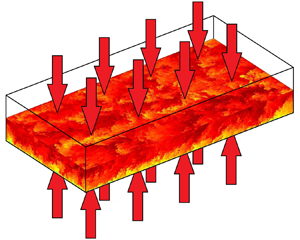
In figure 1, a schematic representation of the lower half of the computational box used can be observed. In this plot, contours of an instantaneous snapshot of the streamwise velocity are represented, coloured by the magnitude of the velocity, and the flow moves from left to right. Periodic conditions are imposed in the streamwise and spanwise boundaries. In previous simulations performed by our group at  ${\textit {Re}}_\tau = 500$,
 $1000$ and
 $2000$, the computational box dimensions were
 $2{\rm \pi} h, 2 h, {\rm \pi}h$ in the streamwise, wall-normal and spanwise directions, respectively. It was stated in Lozano-Durán & Jiménez (Reference Lozano-Durán and Jiménez2014) for the flow field, and in Lluesma-Rodríguez et al. (Reference Lluesma-Rodríguez, Hoyas and Peréz-Quiles2018) for thermal flows, that a computational box with such dimensions is big enough to accurately represent the first-order statistics of the velocity and temperature fields. In order to keep the same resolution for the different Reynolds numbers, the number of collocation points was just multiplied by a factor of two, as was the Reynolds number. However,
 ${\textit {Re}}_\tau = 5000$ is
 $2.5$ times bigger than our closest simulation at
 ${\textit {Re}}_\tau = 2000$. Increasing the number of collocation points only by a factor of two will lead to a poor quality mesh and the results will not be accurate. Since we want to obtain the same mesh resolution as in our previous simulations, the number of collocation points in the
 $x$ and
 $z$ directions is four times higher than the ones in the simulation of
 ${\textit {Re}}_\tau = 2000$. In order to adjust the mesh resolution, the streamwise and spanwise dimensions have been multiplied by a factor of
 $1.6$. Therefore, on one hand, the computational cost will increase due to the high increase in collocation points. But, on the other hand, since the domain is increased in the periodic directions, the number of statistics obtained every time step also increases. Then, the dimensions of the computational box for the present work are set to
 $3.2{\rm \pi} h$,
 $2h$ and
 $1.6{\rm \pi} h$ in the streamwise, wall-normal and spanwise directions, respectively. Coordinates in these directions are denoted by
 $x$,
 $y$ and
 $z$, respectively. The corresponding velocities are
 $U$,
 $V$ and
 $W$, or, using index notation,
 $U_i$. Temperature is represented by
 $T$. However, the transformed temperature,
 $\varTheta$ (defined below), will be used throughout the entire paper. Uppercase letters denote instantaneous flow magnitudes. Using the Reynolds decomposition, one can obtain the averaged value, denoted by an overbar, and the fluctuating part, denoted by a lowercase letter, of the flow magnitudes, i.e.
 $U = \bar {U} + u$. The superscript
 $+$ indicates normalization in wall units, using
 $\nu$ and
 $u_\tau = \sqrt {\tau _w/\rho }$, where
 $\tau _w$ is the mean shear stress and
 $\rho$ is the fluid density. The superscript
 $*$ indicates normalization in outer units, using
 $h$ and
 $U_b$, where
 $U_b$ is the bulk velocity, i.e. the average velocity in time and space.
Schematic representation of the lower half of the computational box. The flow is driven by a pressure gradient,  ${\rm \Delta} P$, from left to right. A constant heat flux,
 $q_w$, is heating both isothermal walls. Contours represent a snapshot of the streamwise velocity field.

2.2. Numerical procedure
The behaviour of turbulent flows is described by the Navier–Stokes equations, which are composed by the continuity and momentum equations,
 \begin{gather} \partial_j U^+_j =0, \end{gather}
 \begin{gather}\partial_t U^+_i + U^+_j\partial_j U^+_i ={-}\partial_i P^+{+} {\frac{1}{{\textit{Re}}_\tau}} \partial_{jj}U^+_i \end{gather}
and the energy equation,
 \begin{equation} \partial_t \varTheta^+{+} U_j^+\partial_j \varTheta^+{=} \frac{1}{{\textit{Re}}_\tau {\textit{Pr}}} \partial_{jj}\varTheta^+{+} U^+{/}\langle U^+ \rangle_{xyz}, \end{equation}
where  $\langle U^+ \rangle _{xyz}$ is the average of
 $U^+$ in time and in the three spatial directions, i.e.
 $\langle U^+ \rangle _{xyz} = U^+_b$. In the energy equation, the transformed temperature,
 $\varTheta = T_w-T$ is used. Since the MBC is used, the temperature in the channel increases linearly in the streamwise direction and periodic conditions cannot be used for
 $T$. Here
 $T_w$ contains the non-periodic part of the temperature, which makes
 $\varTheta$ periodic in the streamwise direction. This allows the use of highly efficient Fourier methods in this direction of the channel. In order to perform the simulation, a variation of the code LISO (Hoyas & Jiménez Reference Hoyas and Jiménez2006; Hoyas & Jiménez Reference Hoyas and Jiménez2008; Avsarkisov et al. Reference Avsarkisov, Hoyas, Oberlack and García-Galache2014; Gandía-Barberá et al. Reference Gandía-Barberá, Hoyas, Oberlack and Kraheberger2018) has been employed. In this variation, the energy equation was introduced and the code was validated by Lluesma-Rodríguez et al. (Reference Lluesma-Rodríguez, Hoyas and Peréz-Quiles2018). The method used in LISO to solve the system of (2.1), (2.2) and (2.3) is the same as the one employed in Kim & Moin (Reference Kim and Moin1987). For this method, the Navier–Stokes equations are transformed into equations for the wall-normal velocity,
 $\varOmega _y$, and the Laplacian of the wall-normal velocity,
 $\varPhi$. After solving them, the other variables are recovered from these two fields using continuity and vorticity equations. The spatial discretization in the
 $x$ and
 $z$ directions is a dealiased Fourier expansion, achieved using the Orszag
 $2/3$ rule (Orszag Reference Orszag1971). In the
 $y$ direction, the discretization employed is a seven-point compact finite difference scheme with fourth-order consistency and extended spectral-like resolution (Lele Reference Lele1992). On the other hand, the temporal discretization employs a third-order semi-implicit Runge–Kutta scheme (Spalart, Moser & Rogers Reference Spalart, Moser and Rogers1991).
2.3. Simulation parameters
Table 1 shows the parameters used for the simulation. Information about the dimensionless numbers, the number of collocation points of the mesh and its resolution in every direction and the time of the simulation, is collected. Regarding the resolution of the mesh in the wall-normal direction, the spacing between points has been set to be proportional to the local isotropic Kolmogorov scale  $\eta = (\nu ^3/\epsilon )^{1/4}$. The increment in
 $y$ is set to be
 ${\rm \Delta} y = 1.5\eta$. Therefore, the wall-normal resolution obtained, in physical space, is
 ${\rm \Delta} y^+_w = 0.20$ in the walls and
 ${\rm \Delta} y^+_c = 8.1$ in the centreline of the channel. On the other hand, the resolution of the mesh in the streamwise and spanwise directions are
 ${\rm \Delta} x^+ \sim 8.18$ and
 ${\rm \Delta} z^+ \sim 4.09$, respectively. These values are set to be the same as in Alcántara-Ávila et al. (Reference Alcántara-Ávila, Hoyas and Pérez-Quiles2018) and similar to many other trusted simulations (Kawamura et al. Reference Kawamura, Ohsaka, Abe and Yamamoto1998; Abe et al. Reference Abe, Kawamura and Matsuo2004; Hoyas & Jiménez Reference Hoyas and Jiménez2006; Avsarkisov et al. Reference Avsarkisov, Hoyas, Oberlack and García-Galache2014; Lluesma-Rodríguez et al. Reference Lluesma-Rodríguez, Hoyas and Peréz-Quiles2018).
Parameters of the simulation. Columns two and three show the friction Reynolds number and the molecular Prandtl number, respectively. Columns four to six show the number of collocations points on each direction of the computational box, after dealiasing in  $x$ and
 $z$. In the next four columns,
 ${\rm \Delta}$ refers to the mesh resolution on each direction and subscripts
 $w$ and
 $c$ refer to the walls and the centreline of the channel. The last column shows the time of the simulation in wash-outs.

In order to initialize the simulation, an initial file of a different case already simulated by our group, at the closest Reynolds number,  ${\textit {Re}}_\tau = 2000$, and the same Prandtl number,
 ${\textit {Pr}} = 0.71$, has been used. The mean temperature has been approximated extrapolating the temperature fields of the cases
 ${\textit {Re}}_\tau = 1000$ and
 $2000$, and the velocity field is converged by running the simulation with a coarse mesh. After the transition phase has passed, and once the values of the viscous stress have converged to a plateau, the statistics of the flow were collected. As a first rule of thumb, the simulation was run for at least 10 wash-outs, where a wash-out is the time needed for an eddy to cross the channel (Hoyas & Jiménez Reference Hoyas and Jiménez2006). The convergence procedure has been done gradually, increasing in three steps the Reynolds number and then increasing the mesh resolution in one direction at a time. For this reason, the computational cost of the convergence procedure is not negligible compared with the total time of the simulation where the flow is statistically steady.
Through all the paper, the results obtained have been compared with the simulations at the same Prandtl number and lower Reynolds number ( $2000$,
 $1000$ and
 $500$) from Alcántara-Ávila et al. (Reference Alcántara-Ávila, Hoyas and Pérez-Quiles2018). Despite the fact that in the work of Pirozzoli et al. (Reference Pirozzoli, Bernardini and Orlandi2016) a different thermal boundary condition is used, the Reynolds number used (
 ${\textit {Re}}_\tau = 4000$) is similar to the
 ${\textit {Re}}_\tau$ of this paper (
 ${\textit {Re}}_\tau = 5000$). For this reason, a comparison of both works has also been performed. Table 2 shows the colours and line styles that have been used in all figures (unless otherwise specified) to distinguish between each simulation.
Line style used to represent each simulation throughout and thermal boundary condition of the case.

In order to confirm that enough statistics have been compiled in the simulation, the heat fluxes have been calculated. These heat fluxes can be obtained from the energy balance equation, which comes from the integration of (2.3),
 \begin{equation} q^+_{total} = \overbrace{\frac{1}{{\textit{Pr}}}\frac{\textrm{d}\bar{\varTheta}^+}{{\textrm{d}y}^+}}^\textrm{{Molecular}} \overbrace{-\overline{v^+\theta^+}}^\textrm{{Turbulent}} = \overbrace{1-\frac{1}{{\textit{Re}}_\tau} \int_0^{y^+}\frac{U_1^+}{\langle U^+\rangle}_{xyz}{\textrm{d}y}}^\textrm{{Total}}. \end{equation}
Total heat flux has been compared with the molecular and turbulent heat fluxes. It has been considered that enough statistics were obtained when the difference between the left- and right-hand sides of (2.4) was below  $10^{-3}$. In figure 2(a), all three heat fluxes are represented for the case of
 ${\textit {Re}}_\tau = 5000$. The dotted line represents the difference between the total heat flux and the sum of the molecular and turbulent heat fluxes. It can be seen that this line has a value of almost zero through all the
 $y^+$ axis. This indicates that enough statistics of the flow have been gathered. In figure 2(b), the same plot is represented for
 ${\textit {Re}}_\tau = 500$,
 $1000$,
 $2000$ and
 $5000$. It is observed that the point of crossoverbetween molecular and turbulent heat flux is approximately constant for different Reynolds numbers and it is located at
 $y^+ \approx 13$. In terms of the
 $y$ coordinate, this means that the viscous layer is smaller when the Reynolds number is increased, as it should be. In the central region of the channel, the turbulent heat flux increases its maximum value when the Reynolds number is increased. The area below the turbulent heat flux line also increases. All this implies that the thermal flow will be more turbulent for higher
 ${\textit {Re}}_\tau$, as expected.
Heat fluxes for (a)  ${\textit {Re}}_\tau = 5000$ and (b)
 ${\textit {Re}}_\tau = 500$,
 $1000$,
 $2000$ and
 $5000$: total (dashed); molecular (solid); and turbulent (dash-doted) heat fluxes. The pointed line represents the difference between the left-hand side and the right-hand side of (2.4). The magenta line represents the maximum molecular heat flux. Colour lines are as in table 2.

3. Results
3.1. Temperature statistics
In the present section, the statistics of the simulation have been obtained and they have been analysed and compared with the ones in the works of Pirozzoli et al. (Reference Pirozzoli, Bernardini and Orlandi2016) and Alcántara-Ávila et al. (Reference Alcántara-Ávila, Hoyas and Pérez-Quiles2018).
The value of the mean temperature,  $\bar {\varTheta }^+$, has been obtained and it is represented in figure 3(a). As was expected, in the viscous layer, all values of
 $\bar {\varTheta }^+$ collapse with the law of the wall:
 $\bar {\varTheta }^+ = {\textit {Pr}}\cdot y^+$. Even the values from Pirozzoli et al. (Reference Pirozzoli, Bernardini and Orlandi2016), where a different boundary condition for the thermal field is used, coincide with the ones obtained in the present work. This shows the universality of turbulence near the wall. However, in the logarithmic layer and in the central region of the channel, the slope of
 $\bar {\varTheta }^+$ tends to decrease with the Reynolds number. For the UHG boundary condition used in Pirozzoli et al. (Reference Pirozzoli, Bernardini and Orlandi2016), the slope is smaller than the one obtained using the MBC.
(a) Mean temperature; the black thin line shows the law of the wall. (b) Here  $\kappa _t$ as a function of
 $Re_\tau$; magenta circles represents the data from Pirozzoli et al. (Reference Pirozzoli, Bernardini and Orlandi2016); cyan triangles are the data from Abe et al. (Reference Abe, Kawamura and Matsuo2004), where the MBC is used, as in this work. Lines are as in table 2.

One parameter that is derived from the mean temperature profile is the von Kármán constant,  $\kappa _t$. In the logarithmic layer,
 $\bar {\varTheta }^+$ can be estimated with a logarithmic equation
 \begin{equation} \bar{\varTheta}^+{=} \frac{1}{\kappa_t}\ln{(y^+)}+B. \end{equation}
The range of validity of (3.1) has been chosen to be  $y^+>70$ and
 $y^+<0.2{\textit {Re}}_\tau$, as suggested by Jiménez (Reference Jiménez2013). Therefore, in this range,
 $\kappa _t$ represents the inverse of the slope of
 $\bar {\varTheta }^+$. This von Kármán constant has been considered independent of the Reynolds number, the type of flow and the boundary conditions by many researchers (Jiménez Reference Jiménez2018). The values of
 $\kappa _t$ are represented in figure 3(b). Results at lower Reynolds numbers from the work of Pirozzoli et al. (Reference Pirozzoli, Bernardini and Orlandi2016) have also been added (magenta circles). In addition, the values of
 $\kappa _t$ obtained in Abe et al. (Reference Abe, Kawamura and Matsuo2004) are represented with cyan triangles. In the work of Abe et al. (Reference Abe, Kawamura and Matsuo2004), the same boundary condition as in this work, the MBC, was used. Results are coherent among all different works.
Here, it is seen that  $\kappa _t$ slightly increases with
 ${\textit {Re}}_\tau$, but, asymptotically, tends to a value slightly above
 $0.44$. One may think that
 $\kappa _t$ depends on the Reynolds number. However, the reason for the variations in the value of
 $\kappa _t$ is that the logarithmic region is not properly developed and it is influenced by the buffer layer and the outer region. A value of
 $\kappa _t = 0.441$ is obtained for
 ${\textit {Re}}_\tau = 5000$. This value is slightly above the von Kármán constant of the velocity field, which ranges between
 $0.38$ and
 $0.4$ (Lozano-Durán & Jiménez Reference Lozano-Durán and Jiménez2014; Lee & Moser Reference Lee and Moser2015). With respect to the UHG, the value of
 $\kappa _t$ increases to
 $0.455$, since the slope of
 $\bar {\varTheta }^+$ is lower, as it was mentioned before. Regarding the constant
 $B$ from (3.1), their values are collected in table 3. Notice that this more or less constant value of
 $B\approx 3$ obtained in all simulations is totally different when the Prandtl number changes (Alcántara-Ávila et al. Reference Alcántara-Ávila, Hoyas and Pérez-Quiles2018).

A visual way of checking how well developed the logarithmic layer is, can be by using the diagnostic function,  $\beta$, defined as
 \begin{equation} \beta = y\partial_y \bar{\varTheta}^+. \end{equation}
If (3.1) holds, then the diagnostic function will have a value of  $1/\kappa _t$ in the logarithmic layer. In figure 4(a), the diagnostic function of the mean temperature is represented. This logarithmic layer appears between the two peaks of the diagnostic function that are obtained in the buffer layer and the outer region. Regarding the peak in the buffer layer, its position is constant at
 $y^+ \approx 12$ and its magnitude continues decreasing with the increase of the Reynolds number. This peak is even lower for the UHG boundary condition. Regarding the peak in the outer region, it is positioned at a constant value in outer coordinates,
 $y/h\approx 0.5$. In the ideal case where a logarithmic region appears perfectly developed, a plateau of value
 $1/\kappa _t$ should be observed approximately between
 $y^+>70$ and
 $y/h<0.2$. This is not observed in any of the cases, since
 $\beta$ increases along the logarithmic layer. However, it is true that the slope of
 $\beta$ tends to zero as the Reynolds number increases. This indicates that higher Reynolds numbers must be simulated in order to be able to find a plateau in the logarithmic layer.


This problem was addressed by Jiménez & Moser (Reference Jiménez and Moser2007). They studied this influence of the Reynolds number in the slope of  $\beta$ on the logarithmic region for the mean velocity profile,
 $U^+$. They used a higher-order truncation in which the diagnostic function had the form
 \begin{equation} \beta = y\partial_y \bar{U}^+{=} \overbrace{\left(\frac{1}{\kappa_\infty} + \frac{\alpha_1}{{\textit{Re}}_\tau}\right)}^{1/\kappa} + \alpha_2\frac{y^+}{{\textit{Re}}_\tau}, \end{equation}
where the Reynolds number dependence is introduced in the term  $\kappa$ and a linear dependence with
 $y/h$ is introduced in the term
 $y^+/{\textit {Re}}_\tau$. This approximation was valid in the range
 $y^+ > 300$ and
 $y/h < 0.45$. The same analysis has been performed here for
 $\bar {\varTheta }^+$. Note that the case
 ${\textit {Re}}_\tau = 500$ does not appear in this analysis since the range where the approximation is valid does not exist. In figure 4(b), a zoom of the diagnostic function together with the approximations of (3.3) are represented.
Values of the parameters of the approximation are presented in table 3. The value of  $\alpha _1$ has been set to
 $150$ as in Jiménez & Moser (Reference Jiménez and Moser2007). While
 $\kappa$ and
 $\kappa _t$ seem to be more or less converged,
 $\alpha _2$ is still larger than the expected limit value of zero for high Reynolds number.
Another parameter that can be derived from the mean thermal field is the Nusselt number,  $Nu$. According to Kawamura et al. (Reference Kawamura, Ohsaka, Abe and Yamamoto1998),
 $Nu$ can be computed as

where  $\langle \varTheta ^+_m\rangle$ is defined as
 \begin{equation} \langle\varTheta^+_m\rangle = \frac{\int^1_0 U^+\varTheta^+ {\textrm{d}y}^*}{\int^1_0U^+ {\textrm{d}y}^*}, \end{equation}
and  is the convective heat transfer coefficient. In figure 5, the obtained Nusselt numbers, as a function of
 ${\textit {Re}}$, are presented. In the range of Reynolds numbers studied, the Nusselt number can be approximated with a power function of
 ${\textit {Re}}$,
 \begin{equation} Nu = 0.031 {\textit{Re}}^{0.796}\quad \textrm{for}\ {\textit{Pr}} = 0.71, \end{equation}
where the coefficient of determination is  $R^2 = 0.99976$, with
 $R^2 = 1$ representing a perfect fit. The data has been compared with results from Pirozzoli et al. (Reference Pirozzoli, Bernardini and Orlandi2016) at lower Reynolds numbers and from Abe et al. (Reference Abe, Kawamura and Matsuo2004). Also, four correlations have been used to compare them with correlation (3.6). Two of them are correlations for turbulent flows in pipes: Dittus & Boelter (Reference Dittus and Boelter1930)
 \begin{equation} Nu = 0.023 {\textit{Re}}_D^{0.8}{\textit{Pr}}^n; \end{equation}
and Gnielinski (Reference Gnielinski1976)
 \begin{equation} Nu = \frac{(f/8)({\textit{Re}}_D-1000){\textit{Pr}}}{1+12.7(f/8)^{1/2}\left({\textit{Pr}}^{2/3}-1\right)}; \end{equation}
where  ${\textit {Re}}_D$ is the diameter of the pipe,
 $n$ is a coefficient of value
 $0.4$ since the fluid is being heated and
 $f$ is proportional to the skin friction coefficient,
 $f = (0.79 \ln ({\textit {Re}}_D)-1.64)^{-2}$. On the other hand, two correlations for constant temperature walls are used. The Kays, Crawford & Weigand (Reference Kays, Crawford and Weigand1980) correlation reads
 \begin{equation} Nu = 0.021 {\textit{Re}}^{0.8}{\textit{Pr}}^{0.5} \end{equation}
and the Sleicher & Rouse (Reference Sleicher and Rouse1975) correlation
 \begin{equation} Nu = 4.8 + 0.0156 {\textit{Re}}^{0.85}{\textit{Pr}}^{0.93} \quad \textrm{for}\ {\textit{Pr}}<0.1. \end{equation}
(a) Nusselt number as a function of  ${\textit {Re}}$. (b) Zoom for the lower Reynolds numbers. Black circles represent the data from Alcántara-Ávila et al. (Reference Alcántara-Ávila, Hoyas and Pérez-Quiles2018) and from this work, magenta squares are the data from Pirozzoli et al. (Reference Pirozzoli, Bernardini and Orlandi2016) and cyan triangles are the data from Abe et al. (Reference Abe, Kawamura and Matsuo2004). Lines represent correlations: black solid (3.6); red dotted Dittus & Boelter (Reference Dittus and Boelter1930) (3.7); orange dashed Gnielinski (Reference Gnielinski1976) (3.8); green dashed Kays et al. (Reference Kays, Crawford and Weigand1980) (3.9); and blue dotted-dashed Sleicher & Rouse (Reference Sleicher and Rouse1975) (3.10).

On one hand, figure 5(a) presents a global image, with all the Reynolds numbers that are being analysed in this work, including the ones from Abe et al. (Reference Abe, Kawamura and Matsuo2004) and Pirozzoli et al. (Reference Pirozzoli, Bernardini and Orlandi2016). Figure 5(b) presents a zoom in the low Reynolds numbers for a better view of the discrepancies between different boundary conditions and correlations in this range of  ${\textit {Re}}$.
One can see that the Nusselt number obtained in Abe et al. (Reference Abe, Kawamura and Matsuo2004) follows the same trend as the ones obtained in this work, since the MBC is employed in both cases. However,  $Nu$ in Pirozzoli et al. (Reference Pirozzoli, Bernardini and Orlandi2016) is slightly higher, since the magnitude of the mean temperature is lower when the UHF thermal condition is used. In other words, the convective heat transfer is lower when the MBC is used.
Regarding the correlations, the ones from Dittus & Boelter (Reference Dittus and Boelter1930) (3.7) and Sleicher & Rouse (Reference Sleicher and Rouse1975) (3.10) overestimate the value of  $Nu$, either because it is for turbulent pipes or because the correlation is valid for lower Prandtl numbers. Correlations from Gnielinski (Reference Gnielinski1976) (3.8) and Kays et al. (Reference Kays, Crawford and Weigand1980) (3.9) adjust much better to the result obtained. They perfectly adjust to the result from Pirozzoli et al. (Reference Pirozzoli, Bernardini and Orlandi2016). Anyway, note that the exponent of
 ${\textit {Re}}$ from correlations (3.7), (3.9) and (3.10) is (or it is close to)
 $0.80$, which is also the case for the correlation proposed in this work (3.6). It is a future work to propose a correlation that also includes the effect of the Prandtl number.
Turbulent intensities are represented in figure 6. The root mean square of the temperature variance,  $\theta '^+$, and the wall-normal heat flux,
 $\overline {v^+\theta ^+}$, are represented in figures 6(a) and 6(b) as a function of outer and inner coordinates, respectively. Also, streamwise heat flux,
 $\overline {u^+\theta ^+}$, is represented in figures 6(c) and 6(d) as a function of outer and inner coordinates, respectively.
Here  $\theta '^+$ and
 $\overline {v^+\theta ^+}$ in (a) outer coordinates and (b) inner coordinates. Here also
 $\overline {u^+\theta ^+}$ in (c) outer coordinates and (d) inner coordinates. Lines are as in table 2.

The main result is that a perfect collapse of the statistics is observed in the inner layer, when the plot is represented in inner coordinates, figures 6(b) and 6(d). On the other hand, when the statistics are represented as a function of the outer coordinates, the collapse is observed in the outer region of the channel.
The maximum values of the turbulent intensities  $\theta '^+$ and
 $\overline {u^+\theta ^+}$ occur in the buffer layer. Their values can be observed in figures 7(a) and 7(b). The peaks increase with Reynolds number, which indicates a more turbulent flow, as was expected. Here
 $\theta '^+$ and
 $\overline {u^+\theta ^+}$ present a linear increase with respect to
 $\log ({\textit {Re}}_\tau )$. Values of the peaks can be obtained with the following correlations:
 \begin{gather} \theta'^+_{max} = 0.112\log({\textit{Re}}_\tau) + 1.82, \end{gather}
 \begin{gather}\overline{u^+\theta^+}_{max} = 0.508\log({\textit{Re}}_\tau) + 3.06. \end{gather}
Maximum value of (a)  $\theta '^+$ and (b)
 $\overline {u^+\theta ^+}$, both as a function of
 ${\textit {Re}}_\tau$. Black line represents correlation (3.11) in (a) and correlation (3.12) in (b). The black circles, data from this work and from Alcántara-Ávila et al. (Reference Alcántara-Ávila, Hoyas and Pérez-Quiles2018); magenta squares, Pirozzoli et al. (Reference Pirozzoli, Bernardini and Orlandi2016); and cyan triangles, Abe et al. (Reference Abe, Kawamura and Matsuo2004).

On the other hand,  $\overline {v^+\theta ^+}$ does not present this linear increase. The peak occurs in the outer region and its value increases slowly as the Reynolds number increases. This was already shown in the magenta line of figure 2(b). Actually,
 $\overline {v^+\theta ^+}$ is bounded by
 $-1$, as can be observed from (2.4). The maximum value of
 $q_{total}^+$ is
 $1$. The turbulent heat flux has its maximum in the core region of the channel. The higher the Reynolds number is, the closer to
 $1$ the value of
 $q_{total}^+$ will be in this core region. Since in this region
 $q_{total}^+ \approx -\overline {v^+\theta ^+}$, for very high Reynolds numbers
 $-\overline {v^+\theta ^+}$ will be close to
 $1$.
Regarding the UHG case, the peaks of the three intensities have a lower absolute value, which indicates a less turbulent thermal field than the one obtained using the MBC. Lower Reynolds number cases have been also represented to see how this feature happens for all simulations, obtaining the same tendency. Also, data from Abe et al. (Reference Abe, Kawamura and Matsuo2004) has been added. This has been done to verify the results, since Abe et al. (Reference Abe, Kawamura and Matsuo2004) also used the MBC. Effectively, the results are very similar, and the small differences (less than  $1\,\%$) can be due to numerical discrepancies or different mesh resolution.
In a similar way that the mean velocity and temperature are studied through the diagnostic function in the logarithmic layer, velocity intensities can be analysed through Townsend's attached eddy hypothesis (Townsend Reference Townsend1976). This hypothesis is valid for high Reynolds number flows, in a certain region of  $y$, where the velocity intensities satisfy
 \begin{gather} {u'^2}^+{=} A_1 - B_1 \log\left(y/h\right), \end{gather}
 \begin{gather}{v'^2}^+{=} A_2, \end{gather}
 \begin{gather}{w'^2}^+{=} A_3 - B_3 \log\left(y/h\right), \end{gather}
 \begin{gather}\overline{u'v'}^+{=} -1. \end{gather}
Analogously, due to the high correlation between  $u'^+$ and
 $\theta '^+$, one may think that Townsend's hypothesis is valid for the thermal field when
 $u'^+$ is replaced by
 $\theta '^+$. Doing this, the following relations are obtained:
 \begin{gather} {\theta'^2}^+{=} A_4 - B_4 \log\left(y/h\right), \end{gather}
 \begin{gather}\overline{u'\theta'}^+{=} A_5 - B_6 \log\left(y/h\right), \end{gather}
 \begin{gather}\overline{v'\theta'}^+{=} -1. \end{gather}
It has already been shown that the minimum value of  $\overline {v'\theta '}^+$ tends to
 $-1$ in a wider range of
 $y/h$ when the Reynolds number is increased (figures 6a and 6b). This is in accordance with (3.19). Regarding
 ${\theta '^2}^+$ and
 $\overline {u'\theta '}^+$, their diagnostic functions can be observed in figures 8(a) and 8(b), respectively. If Townsend's criteria can be applied to the thermal field, there should be a plateau in the
 $y^+\partial _y {\theta '^+}^2$ and
 $y^+\partial _y \overline {u^+\theta ^+}$ profiles. For these values of
 ${\textit {Re}}_\tau$ there is no evidence of this plateau, although the trends may indicate that for higher Reynolds numbers it may appear in the logarithmic layer.
Diagnostic function for (a)  ${\theta '^2}^+$ and (b)
 $\overline {u'\theta '}^+$. Lines are as in table 2.

Another important parameter for modelling of thermal flows is the turbulent Prandtl number,  ${\textit {Pr}}_t$. It is defined as the ratio between the momentum eddy diffusivity,
 $\nu _t$, to the thermal eddy diffusivity,
 $\kappa _t$,
 \begin{equation} {\textit{Pr}}_t = \frac{\nu_t}{\kappa_t}=\frac{\overline{uv}}{\bar{v\theta}} \frac{\textrm{d}\bar{\varTheta}/{\textrm{d}y}}{\textrm{d}\bar{U}/{\textrm{d}y}}. \end{equation}
In figure 9,  ${\textit {Pr}}_t$ is shown as a function of
 $y^+$. In the viscous layer, it can be seen how
 ${\textit {Pr}}_t$ is close to
 $1$ and constant for all values of Reynolds numbers. This confirms the well known law that states
 ${\textit {Pr}}_t \approx 1$ in the wall for medium molecular Prandtl numbers (Kawamura et al. Reference Kawamura, Ohsaka, Abe and Yamamoto1998; Alcántara-Ávila et al. Reference Alcántara-Ávila, Hoyas and Pérez-Quiles2018). Some differences are observed with respect to the
 ${\textit {Pr}}_t$ obtained by Pirozzoli et al. (Reference Pirozzoli, Bernardini and Orlandi2016). However, in the buffer layer and logarithmic region, all values of
 ${\textit {Pr}}_t$ seem to collapse, including the ones obtained in Pirozzoli et al. (Reference Pirozzoli, Bernardini and Orlandi2016). In the outer layer, values of
 ${\textit {Pr}}_t$ decrease. In conclusion, there have not been observed new behaviours of the turbulent Prandtl number for the Reynolds number
 ${\textit {Re}}_\tau = 5000$.
Turbulent Prandtl number. Lines are as in table 2.

3.2. Turbulent budgets
In this section, budgets of the temperature variance,  $k_\theta =1/2 \theta ^2$, the dissipation rate of the temperature variance,
 $\varepsilon _\theta = ({1}/{{\textit {Pr}}})\overline {\partial _i \theta \partial _i \theta }$ and the turbulent heat fluxes,
 $\overline {u\theta }$ and
 $\overline {v\theta }$, are presented. The equation for the budget of
 $k_\theta$ is
 \begin{equation} \frac{\textrm{D}\overline{k_\theta}}{\textrm{D} t}=P+T+V+\varepsilon_\theta, \end{equation}
where  ${\textrm {D}}/{\textrm {D} t}$ is the mean substantial derivative and
 $P$ is the production term,
 $T$ is the turbulent diffusion,
 $V$ is the viscous diffusion and
 $\varepsilon _\theta$ is the dissipation term. Each term is defined as follows:
 \begin{gather} P ={-}\overline{v\theta} \partial_y\bar{\varTheta}, \end{gather}
 \begin{gather}T ={-}\tfrac{1}{2}\partial_y \overline{\theta^2v}, \end{gather}
 \begin{gather}V = \frac{1}{2Pr}\partial^2_{yy}\overline{\theta^2}, \end{gather}
 \begin{gather}\varepsilon_\theta ={-} \frac{1}{Pr,}\overline{\partial_i \theta\partial_i \theta}. \end{gather}
For  $\varepsilon _\theta$, the following budget equation is obtained:
 \begin{equation} \frac{\textrm{D}\overline{\varepsilon_\theta}}{\textrm{D} t}=P_m+P_{mg}+P_{g}+P_{t}+T_{t}+ V_{\varepsilon_{\theta}}+\varepsilon_{\theta 1}, \end{equation}
where  $P_m$,
 $P_{mg}$,
 $P_g$ and
 $P_t$ are the mixed production, mean gradient production, gradient production and turbulent production, respectively. Here
 $T_t$,
 $V_{\varepsilon _{\theta }}$ and
 $\varepsilon _{\theta 1}$ are the turbulent diffusion, molecular diffusion and dissipation terms. Their definitions are given by
 \begin{gather} P_m ={-}\frac{2}{Pr}\overline{\partial_i v\partial_i \theta} \partial_y \bar{\varTheta}, \end{gather}
 \begin{gather}P_{mg} ={-} \frac{2}{Pr} \overline{\partial_x \theta \partial_y \theta} \partial_y\bar{U}, \end{gather}
 \begin{gather}P_{g} ={-} \frac{2}{Pr} \overline{v\partial_y \theta} \partial^2_{yy} \bar{\varTheta}, \end{gather}
 \begin{gather}P_{t} ={-} \frac{2}{Pr} \overline{\partial_i \theta \partial_j \theta \partial_j u_i }, \end{gather}
 \begin{gather}T_{t} ={-} \frac{1}{Pr} \partial_y \overline{v \partial_i \theta \partial_i \theta }, \end{gather}
 \begin{gather}V_{\varepsilon_{\theta}} =\frac{1}{Pr^2} \partial^2_{yy} \varepsilon_0, \end{gather}
 \begin{gather}\varepsilon_{\theta 1} ={-} \frac{2}{Pr^2} \overline{\partial^{2}_{kj}\theta\partial^{2}_{kj}\theta}. \end{gather}
Finally, the budget equations for the turbulent heat fluxes are
 \begin{equation} \frac{\textrm{D}\overline{u_i\theta}}{\textrm{D} t}=P_{i}+T_{i}+V_{i}+\varPi^{s}_{i}+\varPi^{d}_{i}+\varepsilon_{i}, \end{equation}
where each term, from left to right, is the production, turbulent diffusion, viscous diffusion, pressure–temperature gradient correlation, pressure diffusion and dissipation. These terms are defined as
 \begin{gather} P_{i} ={-}\overline{u_iv}\partial_{y}\bar{\varTheta} - \overline{v\theta}\partial_{y}\overline{U_i}, \end{gather}
 \begin{gather}T_{i} ={-}\partial_{x_k}\overline{u_iu_k\theta}, \end{gather}
 \begin{gather}V_{i} =\nu \partial_{x_k}\left( \overline{\theta \partial_{x_k}u_i}+\frac{1}{Pr} \overline{u_i \partial_{x_k}\theta} \right), \end{gather}
 \begin{gather}\varPi_{i}^{s} =\overline{p\partial_{x_i}\theta}, \end{gather}
 \begin{gather}\varPi_{i}^{d} ={-}\partial_{x_k}(\delta_{ki}\overline{p\theta}), \end{gather}
 \begin{gather}\varepsilon_{i} ={-}\nu \left(1+\frac{1}{Pr}\right) \overline{\partial_{x_k}u_i\partial_{x_k}\theta}, \end{gather}
where  $\delta _{ij}$ is Kronecker's delta and repeated index implies summation over
 $k=1$,
 $2$,
 $3$.
Figure 10 shows the different budget terms for all cases that use the MBC in table 2. Figure 10(a) represents the budget terms of  $k_\theta$. The term
 $\nu /u^{2}_\tau \theta ^2_\tau$ has been used to normalize the data. In figure 10(b), the budgets of
 $\varepsilon _\theta$ are represented. For these budget terms,
 $\nu ^3/u^{4}_\tau \theta ^2_\tau$ have been used for the normalization. In addition, the four production terms of
 $\varepsilon _\theta$ have been added. This summation has been represented as a single production term to facilitate the visualization and interpretation. Finally, figures 10(c) and 10(d) show the budget terms of
 $\overline {u\theta }$ and
 $\overline {v\theta }$, respectively. These data have been normalized by
 $\nu /u^{3}_\tau \theta _\tau$. The idea of this section is to study if these normalizations, proposed in Lluesma-Rodríguez et al. (Reference Lluesma-Rodríguez, Hoyas and Peréz-Quiles2018) and Kozuka, Seki & Kawamura (Reference Kozuka, Seki and Kawamura2009), work for the different
 ${\textit {Re}}_\tau$ so that the data collapse in all the channels.
Budgets of (a) temperature variance,  $\overline {k_\theta }$, (b) dissipation rate of the temperature variance,
 $\overline {\varepsilon _\theta }$, (c) streamwise heat flux,
 $\overline {u\theta }$ and (d) wall-normal heat flux,
 $\overline {v\theta }$. Symbols denote budget terms: production or sum of productions in panel (b), (triangle up); turbulent diffusion (circle); viscous diffusion (square); dissipation (triangle down); pressure strain (star); and pressure diffusion (diamond). The black line with value
 $0$ is the summation of all terms. Lines are as in table 2.

For  $k_\theta$, figure 10(a), all terms collapse for
 $y^+ > 10$. In the buffer layer, the turbulent diffusion terms present small discrepancies between all cases. Furthermore, in the viscous layer there are big differences between each viscous diffusion and the dissipation terms. The absolute values of these terms increase with the Reynolds number.
The reason for the discrepancies in the wall for the viscous diffusion and the dissipation terms can be understood by doing a Taylor series approximation as in Kawamura et al. (Reference Kawamura, Ohsaka, Abe and Yamamoto1998). Here  $\theta '^+$ can be approximated by
 \begin{equation} \theta'^+{=} {\textit{Pr}}(b_\theta y^+{+} c_\theta {y^+}^2 + \cdots). \end{equation}
Therefore, near the wall,  $\theta '^+ \approx {\textit {Pr}}\cdot b_\theta \cdot y^+$. In figure 11(a) it is shown how this is true for approximately
 $y^+ < 3$. The values of
 $b_\theta$ are collected in table 4.
(a) Here  $\theta '^+/{\textit {Pr}}$ and (b)
 $\overline {u^+\theta ^+}/{\textit {Pr}}$ in wall coordinates. Zooms of the viscous layer. Lines are as in table 2.

First column shows the case. Values of  $b_\theta$ are in second column. Third and fourth columns show the value of
 $V^+|_{y=0}$ obtained from the statistics and calculated with (3.43), respectively.

On the other hand, one can approximate the value of the viscous diffusion term,  $V$, in the wall as follows:
 \begin{equation} \left.V\right|_{y=0} = \left.\frac{1}{2 {\textit{Pr}}}\partial_{yy}\overline{\theta'^2}\right|_{y=0} . \end{equation}
Using approximation (3.41), the value of  $V$ in the wall is
 \begin{equation} \left.V^+\right|_{y=0} \approx {\textit{Pr}}\cdot b_\theta^2 . \end{equation}
The result of the approximation is almost the actual value (table 4). In all cases the error is lower than  $1\,\%$. Therefore, the reason why this term of the turbulent budget does not scale in the wall comes from the differences in the
 $b_\theta$ terms. This term represents the slope of
 $\theta '^+/{\textit {Pr}}$ near the wall. Looking at the zoom in figure 11(a), one can see that, effectively, the lines of
 $\theta '^+/{\textit {Pr}}$ are parallel, but they do not collapse. The differences in
 $V$ for cases with the same Prandtl number is due to the increase in the slope of
 $\theta '^+$ with the Reynolds number. One may think that this value of
 $b_\theta$ converges for very large Reynolds numbers, as it may look from the trend in table 4. However, it was seen in figure 6(b) that the maximum value of
 $\theta '^+$ always increases with
 ${\textit {Re}}_\tau$, at least for
 ${\textit {Re}}_\tau \le 5000$. Because the position of the peak was constant in
 $y^+$, the slope of
 $\theta '^+$ has to be higher for larger
 ${\textit {Re}}_\tau$. In other words, as long as the peak of
 $\theta '^+$ increases with
 ${\textit {Re}}_\tau$,
 $b_\theta$ will also increase and
 $V$ cannot scale at the wall. It was observed in Alcántara-Ávila & Hoyas (Reference Alcántara-Ávila and Hoyas2020), that for high Prandtl numbers, the peak value of
 $\theta '^+$ was approximately constant, which yielded an approximately constant value of
 $b_\theta$ and, therefore, a much better scaling of the viscous diffusion term near the wall. This suggests that the effect of reaching a constant behaviour of
 $\theta '^+$ in the near-wall region, and thus, a good scaling of
 $V^+$ at the wall, only depends on the thermal field. The same analysis can be done for the dissipation term, since, at the wall,
 $V = -\varepsilon _\theta$.
In the case of  $\varepsilon _\theta$ (figure 10b) the scaling failures appear in the buffer layer for the sum of production terms and the dissipation. This increase of the production terms was already reported in other works such as Abe & Antonia (Reference Abe and Antonia2009).
For the budgets of  $\overline {u\theta }$ (figure 10c), the viscous diffusion and dissipation terms do not scale near the wall, like in
 $\overline {k_\theta }$. Actually, the phenomenon is very similar and it can be studied in the same way. The streamwise velocity fluctuation and heat flux can be approximated as in Kawamura et al. (Reference Kawamura, Ohsaka, Abe and Yamamoto1998),
 \begin{gather} u'^+{=} b_1 y^+{+} c_1 {y^+}^2 + \cdots , \end{gather}
 \begin{gather}\overline{u^+\theta^+} = {\textit{Pr}}\left(b_{1\theta} {y^+}^2 + c_{1\theta} {y^+}^3 + \cdots\right). \end{gather}
Therefore, near the wall,  $u'^+ \approx b_1 y^+$ and
 $\overline {u^+\theta ^+} \approx {\textit {Pr}}\cdot b_{1\theta }\cdot {y^+}^2$. The approximation is shown for
 $\overline {u^+\theta ^+}$ in figure 11(b). It presents a good estimation up to
 $y^+<4$. A similar picture was obtained for
 $u'^+$ with good agreement for
 $y^+<3$, not shown for brevity. The viscous diffusion of
 $\overline {u\theta }$,
 $V_u$, has the following form at the wall:
 \begin{equation} \left.V_u\right|_{y=0} = \left.\nu \partial_y\left(\overline{\theta\partial_y u} + \frac{1}{{\textit{Pr}}}\overline{u\partial_y \theta}\right)\right|_{y=0} . \end{equation}
Using the chain rule, we obtain
 \begin{align} \left.V_u\right|_{y=0} &= \nu \left(\overline{\partial_y \theta \partial_y u} + \overline{\theta \partial_{yy} u} \right. \end{align}
 \begin{align} &\quad +\left.\left.\frac{1}{{\textit{Pr}}}\overline{\partial_y u\partial_y \theta} + \frac{1}{{\textit{Pr}}}\overline{u\partial_{yy} \theta}\right)\right|_{y=0} . \end{align}
Since  $\overline {\theta \partial _{yy} u} = \overline {u\partial _{yy} \theta } = 0$ at the wall, one gets
 \begin{align} \left.V_u\right|_{y=0} &= \left.\nu \frac{{\textit{Pr}} + 1}{{\textit{Pr}}} \left(\overline{\partial_y \theta \partial_y u} + \overline{\partial_y u\partial_y \theta}\right)\right|_{y=0} \end{align}
 \begin{align} &= \left.\nu \frac{{\textit{Pr}} + 1}{{\textit{Pr}}}\partial_{yy}\overline{u\theta}\right|_{y=0} . \end{align}
Using the definition from (3.45) we finally obtain
 \begin{equation} \left.V^+_u\right|_{y=0} = \left({\textit{Pr}}+1\right)b_{1\theta} . \end{equation}
For  $V^+_u|_{y=0}$ the errors are lower than
 $3\,\%$ for all cases (see table 5), proving a good accuracy of the approximation. Therefore, while
 $b_{1\theta }$ increases with the Reynolds number, the value of
 $V^+_u$ will also increase at the wall. This will occur as long as the peak of
 $\overline {u^+\theta ^+}$ keeps increasing (figure 6d).
First column shows the case. Values of  $b_{1\theta }$ are in second column. Third and fourth columns show the value of
 $V^+_u|_{y=0}$ obtained from the statistics and calculated with (3.51), respectively.

As a conclusion, the scaling failure near the wall of  $V^+$ and
 $V^+_u$ is due to the increase of the peak of
 $\theta '^+$ and
 $\overline {u^+\theta ^+}$, respectively.
Regarding the turbulent budgets of  $\overline {v^+\theta ^+}$ (figure 10d), small scaling failures appear in the buffer layer for the production and pressure strain terms. Near the wall, bigger discrepancies appear for the pressure strain and pressure diffusion terms. The pressure strain term can be written as
 \begin{equation} \varPi_{v}^{s} = \overline{p\partial_y\theta} . \end{equation}
The reason why  $\varPi _{v}^{s}$ does not scale in the wall is again because the term
 $\overline {p\partial _y\theta }$ has a peak at a constant
 $y^+$ and it continuously increases with the Reynolds number; not shown here for brevity.
As a general comment, the budgets of  $\overline {k_\theta }$ and
 $\overline {u^+\theta ^+}$ are very similar due to the high correlation between
 $u'^+$ and
 $\theta '^+$. Near the wall, the energy enters the thermal flow through viscous diffusion and it is extracted by dissipation. Also, the peak of the production term is constant for different Reynolds numbers. For
 $\overline {k_\theta }$, the value of
 $P$ is
 ${\textit {Pr}}/4$, as noted by Abe & Antonia (Reference Abe and Antonia2017). On the other hand, there is not a clear scaling with
 ${\textit {Pr}}$ for the peak of
 $P_1$. In the case of the budgets of
 $\overline {v^+\theta ^+}$, a similar picture to that of
 $\overline {u^+v^+}$ is obtained (not shown here for brevity), again, due to the high correlation between
 $u'^+$ and
 $\theta '^+$. In this case, the energy is introduced by the pressure strain and it is extracted by the pressure diffusion.
A different picture is obtained above the buffer layer, up to approximately  $y/h = 0.4$. Figure 12 shows the same turbulent budgets as before, premultiplied by
 $y^+$. In a perfectly developed logarithmic layer, the kinetic energy production scales with
 $1/y^+$ (Hoyas & Jiménez Reference Hoyas and Jiménez2008). Note that this is approximately true for the dominant budgets of
 $\overline {k_\theta }$,
 $\overline {u\theta }$ and
 $\overline {v\theta }$. Therefore, a much better comparison between the dominant budget terms above the buffer layer can be done. As in the near-wall region, production is the dominant budget term of
 $\overline {k_\theta }$, which is compensated by the dissipation term. However, in the case of
 $\overline {u\theta }$, and also for
 $\overline {v\theta }$, it is the pressure strain what compensates the production term.
Budgets of the  $y^+$-premultiplied (a) temperature variance,
 $y^+\overline {k_\theta }$, (b) dissipation rate of the temperature variance,
 $y^+\overline {\varepsilon _\theta }$, (c) streamwise heat flux,
 $y^+\overline {u\theta }$ and (d) wall-normal heat flux,
 $y^+\overline {v\theta }$. Symbols denote budget terms: production or sum of productions in (b), (triangle up); turbulent diffusion (circle); viscous diffusion (square); dissipation (triangle down); pressure strain (star); and pressure diffusion (diamond). The black line with value
 $0$ is the summation of all terms. Lines are as in table 2.

In the centre of the channel (above  $y/h=0.4$) the velocity and temperature flatten and all production terms tend to zero. Turbulent diffusion becomes the dominant budget of
 $\overline {k_\theta }$ and it is compensated by the dissipation.
As a final comment, there are no noticeable changes in the behaviour of the turbulent budgets with respect to lower Reynolds number cases. In the present study all cases analysed had the same Prandtl number. However, the value of  $b_\theta$ and
 $b_{1\theta }$ decrease drastically for
 ${\textit {Pr}} \le 0.2$ (Kawamura et al. Reference Kawamura, Ohsaka, Abe and Yamamoto1998). In Alcántara-Ávila et al. (Reference Alcántara-Ávila, Hoyas and Pérez-Quiles2018) the effects of low Prandtl numbers on the scaling were shown. A similar analysis of the turbulent budgets for high Prandtl numbers is reported in Alcántara-Ávila & Hoyas (Reference Alcántara-Ávila and Hoyas2020).
4. Conclusions
A DNS of a thermal channel flow at  ${\textit {Re}}_\tau = 5000$ has been conducted for the first time. The MBC has been used. The Prandtl number of air,
 $0.71$, was used. The results obtained are compared with other simulations using the same Prandtl number and lower Reynolds numbers:
 ${\textit {Re}}_\tau = 500$,
 $1000$ and
 $2000$. Also, the simulation with closest Reynolds number,
 ${\textit {Re}}_\tau = 4000$, is used to compare results. In that simulation the UHG boundary condition was used. A comparison between both boundary conditions is provided.
The mean temperature is calculated and its diagnostic function still does not show a plateau in the logarithmic layer. Higher Reynolds numbers are needed in order to properly study the behaviour of the thermal field in this logarithmic region. The von Kármán constant presents an asymptotic behaviour with an increasing Reynolds number and it tends to converge at a value of approximately  $0.44$. The reason why
 $\kappa _t$ is not constant is attributed to the influence of the inner and outer regions on the logarithmic region, since for these Reynolds numbers this logarithmic region is small. This effect of the Reynolds number on the logarithmic layer is also studied through a slightly different diagnostic function. For this case, a new term that contemplates the dependence of the Reynolds number is introduced. Effectively, the value of this term tends towards zero when the Reynolds number is increased.
A new correlation for the Nusselt number is provided. This correlation is valid for turbulent thermal channel flows,  ${\textit {Pr}} = 0.71$ and
 $500\le {\textit {Re}}_\tau \le 5000$. It has been compared with classical Nusselt number correlations. Regarding the turbulent Prandtl number, there are not relevant results at
 ${\textit {Re}}_\tau = 5000$ and the trends of
 ${\textit {Pr}}_t$ are the same as for lower Reynolds numbers.
Thermal intensities increase with the Reynolds number and the values of the inner peaks increase logarithmically with  ${\textit {Re}}_\tau$ for
 $\theta '^+$ and
 $\overline {u^+\theta ^+}$. Here
 $\overline {v^+\theta ^+}$ tends to have a minimum value close to
 $-1$ in a wider range of
 $y^+$ for high Reynolds numbers. This agrees with the application of Townsend's hypotheses to the thermal intensities. However,
 ${\theta '^+}^2$ and
 $\overline {u^+\theta ^+}$ do not present a logarithmic dependence at any region of
 $y$ as it indicates Townsend's hypotheses. A remarkable difference between the MBC and UHF thermal conditions is observed in the temperature intensities. Magnitudes of these intensities are higher when the MBC is used, meaning that a more turbulent flow is obtained.
Turbulent budgets are presented and scaling failures are analysed. The most relevant scaling failures are the ones that occur near the wall for the dissipation and viscous diffusion terms of  $k_\theta$ and
 $\overline {u\theta }$. These scaling failures are a direct result of the increase of the inner peak of
 $\theta '^+$ and
 $\overline {u^+\theta ^+}$, respectively. In the cases of the budgets of
 $\overline {v^+\theta ^+}$, the scaling failures occur in the pressure strain and pressure diffusion terms. In the same way, this occurs for the increase of the inner peak of the variable
 $\overline {p^+\partial _{y^+}\theta ^+}$.
Availability of data
The raw data that support the findings of this study are available from the corresponding author upon reasonable request. One point statistics can be downloaded from the web page of our group: http://personales.upv.es/serhocal/
Acknowledgements
This work was supported by RTI2018-102256-B-I00 of MINECO/FEDER. F.A.A. is partially funded by GVA/FEDER project ACIF2018. The computations of the new simulations were made possible by a generous grant of computing time from the Barcelona Supercomputing Centre, reference IM-2019-3-0021. We are grateful to Messrs Kawamura, Pirozzoli, Bernardini and Orlandi for providing us with copies of their original data.
Declaration of interests
The authors report no conflict of interest.



