1. Introduction
Vorticity in inviscid fluids governed by incompressible Euler equations has remarkable geometric and Lagrangian properties that were derived in classic works of Cauchy (Reference Cauchy1815), von Helmholtz (Reference von Helmholtz1858), Weber (Reference Weber1868), Kelvin (Reference Kelvin1868) and others. In a Hamiltonian formulation of the ideal fluid equations, these properties arise from an infinite-dimensional particle-relabelling symmetry of the action function (Salmon Reference Salmon1988) and they are intimately related to the modern geometric view of the Euler equations as governing geodesic flow on the space SDiff of volume-preserving transformations (Arnold Reference Arnold1966; Besse & Frisch Reference Besse and Frisch2017). These Lagrangian properties of vorticity have often been invoked in theories of turbulent energy dissipation, especially by Taylor (Reference Taylor1937, Reference Taylor1938) and Taylor & Green (Reference Taylor and Green1937). In these papers Taylor suggested that vortex lines which are materially advected by a turbulent flow should be lengthened by random stretching and mean-square vorticity thus enhanced by conservation of circulations. Taylor admitted, however, that vortex lines move as material lines and circulations on material loops are conserved only for ideal smooth Euler flows and these properties may be substantially modified by fluid viscosity. Subsequent works have confirmed that statistical and dynamical properties of vortex lines and material lines are quite distinct in turbulent flows. For example, Lüthi, Tsinober & Kinzelbach (Reference Lüthi, Tsinober and Kinzelbach2005), Guala et al. (Reference Guala, Lüthi, Liberzon, Tsinober and Kinzelbach2005, Reference Guala, Liberzon, Lüthi, Kinzelbach and Tsinober2006) have found in an experimental study of nearly homogeneous, isotropic turbulence that vortex stretching rates are smaller than rates of material-line stretching when both are measured along the trajectories of neutrally buoyant polystyrene particles. A closely related numerical study of isotropic turbulence by Johnson & Meneveau (Reference Johnson and Meneveau2016) has shown that these differences in stretching rates extend even to the rare fluctuations described by large-deviations theory. Johnson et al. (Reference Johnson, Hamilton, Burns and Meneveau2017) have furthermore shown that large-deviation statistics of vortex stretching rates and material line-stretching rates are also distinct in a turbulent channel flow. It might be inferred from these negative findings that the remarkable Lagrangian properties enjoyed by vorticity for smooth Euler flows have no relevance for physical turbulent flows, even at very high Reynolds numbers.
Recently, however, Constantin & Iyer (Reference Constantin and Iyer2008, Reference Constantin and Iyer2011) have shown that the deep geometric and Lagrangian properties of vorticity for Euler dynamics fully extend to viscous Navier–Stokes solutions within a stochastic framework. In the setting of their theorems, a random white noise is added to the evolution equations for Lagrangian fluid particles and this noise averaged over to represent mathematically the viscous diffusion of momentum. Constantin & Iyer (Reference Constantin and Iyer2008, Reference Constantin and Iyer2011) showed that every Navier–Stokes solution satisfies stochastic generalizations of the Weber formula (Weber Reference Weber1868), the conservation of circulations (Kelvin Reference Kelvin1868), the Cauchy formula and conserved Cauchy invariants (Cauchy Reference Cauchy1815), with all of these results reducing in the inviscid limit to those satisfied by smooth Euler solutions. Eyink (Reference Eyink2010) has shown that these properties follow from particle-relabelling symmetry in a stochastic least-action formulation of incompressible Navier–Stokes and Rezakhanlou (Reference Rezakhanlou2016) has discussed the Constantin–Iyer results in the setting of stochastic symplectic flows in phase space. It should be noted that the same stochastic Lagrangian representation of vorticity as Constantin & Iyer (Reference Constantin and Iyer2008) was obtained even earlier by Rapoport (Reference Rapoport2002, § 11), as the corollary of a more general result for Navier–Stokes equations on a compact Riemannian manifold without boundary. This level of generality is not required for most applications in fluid mechanics and, unfortunately, obscures the simplicity of the results for Navier–Stokes flows in flat Euclidean space.
The established Lagrangian properties of vorticity hold both for boundary free Navier–Stokes flows (Constantin & Iyer Reference Constantin and Iyer2008) and for wall-bounded flows with stick boundary conditions (b.c.) on the fluid velocity (Constantin & Iyer Reference Constantin and Iyer2011). In the latter case, however, Constantin & Iyer (Reference Constantin and Iyer2011) were able to show only existence of suitable boundary conditions in their Lagrangian formulation, without an explicit, concrete construction. We solve that problem here by exploiting the Kuz'min–Oseledets formulation of the incompressible Navier–Stokes equation in terms of the vortex-momentum density (Kuz'min Reference Kuz'min1983; Oseledets Reference Oseledets1989). We recall that vortex momentum is the total impulse required to set a compact vortex into motion (Batchelor Reference Batchelor2000, § 7.2) and its density can be interpreted physically as the vortex-momentum per volume when the fluid velocity field is represented by a continuous distribution of infinitesimal vortex rings. The theory of Constantin & Iyer (Reference Constantin and Iyer2008, Reference Constantin and Iyer2011) can be understood as a stochastic representation of viscosity in the Kuz'min–Oseledets formulation, which we show extends readily to wall-bounded flows. In this setting the Constantin & Iyer (Reference Constantin and Iyer2011) theory provides an infinite set of stochastic Cauchy invariants for Navier–Stokes solutions, which permit an exact representation of the vorticity at any interior point in terms of vorticity at the wall. We further discuss some relations of Constantin & Iyer (Reference Constantin and Iyer2011) with the standard Eulerian theory of vorticity generation at solid boundaries due to Lighthill (Reference Lighthill and Rosenhead1963) and Morton (Reference Morton1984), which relates inviscid generation of vorticity to tangential pressure gradients at the wall. Wall-bounded turbulence driven by an imposed pressure-gradient or free stream velocity differs from homogeneous, isotropic turbulence in that energy dissipation requires not just random stretching of vortex lines but in fact an organized, coherent transport of vorticity. Indeed it follows from the Lighthill–Morton theory that a mean pressure drop down a pipe or channel implies the production of spanwise vorticity and a mean viscous flux of such vorticity away from the wall. This exact relation has been previously exploited in developing turbulent drag-control methods aimed at modifying the boundary vorticity flux (Koumoutsakos Reference Koumoutsakos1999; Zhao, Wu & Luo Reference Zhao, Wu and Luo2004).
It is in fact a paradigm in the study of quantum fluids that effective drag in an otherwise non-dissipative superfluid is associated to cross-stream motion of quantized vortex lines by the so-called ‘Josepson-Anderson relation’; see Josephson (Reference Josephson1962), Anderson (Reference Anderson1966), Packard (Reference Packard1998) and Varoquaux (Reference Varoquaux2015) for reviews. Such a result was already anticipated for classical turbulent pipe flow by Taylor (Reference Taylor1932) and more systematically discussed in that context by Huggins (Reference Huggins1970, Reference Huggins1994) and Eyink (Reference Eyink2008). The physical basis of the relation is very general and follows just from the local conservation of momentum, rewritten as
 \begin{equation} \partial_t u_i =\tfrac{1}{2}\epsilon_{ijk} \Sigma_{jk} - \partial_i h \end{equation}
for a suitable anti-symmetric matrix  $\boldsymbol{\Sigma}$ and potential
 $h.$ For example, the incompressible Navier–Stokes equation when rewritten in this manner has these quantities given by
 \begin{equation} \Sigma_{ij} = u_i\omega_j - u_j\omega_i + \nu\left(\frac{\partial\omega_i}{\partial x_j}- \frac{\partial\omega_j}{\partial x_i}\right), \quad h = p +\frac{1}{2}|{{\boldsymbol{u}}}|^{2}. \end{equation}
Other fluid systems will have different contributions here, e.g. a body force  ${\boldsymbol {f}}$ from the stress of a polymer additive will contribute a term
 $\Sigma _{ij}=\epsilon _{ijk}\,f_k$ from the Magnus effect. Taking the curl of (1.1) in general leads to the equation for local conservation of vorticity
 \begin{equation} \partial_t \omega_j + \partial_i \Sigma_{ij} =0 , \end{equation}
where  $\Sigma _{ij}$ gives the flux of the
 $j$th component of vorticity in the
 $i$th coordinate direction. For Navier–Stokes, (1.3) is equivalent to the equation of von Helmholtz (Reference von Helmholtz1858), with contributions to the vorticity flux in (1.2a,b) arising from nonlinear advection, vortex stretching and viscous diffusion, respectively. As pointed out by Taylor (Reference Taylor1932) for a two-dimensional turbulent pipe flow and by Huggins (Reference Huggins1994) for more general statistically steady flows, the average of (1.1) implies a pointwise relation between mean vorticity transport and the mean gradient of (generalized) pressure, i.e.
 \begin{equation} \bar{\Sigma}_{ij} = \epsilon_{ijk} \partial_k \overline{\left( p+\tfrac{1}{2}|{{\boldsymbol{u}}}|^{2}\right)} , \end{equation}
with  $\partial _i \bar {\Sigma }_{ij}=0.$ There is an inward flux of spanwise vorticity not only at the wall, as predicted by the Lighthill–Morton theory, but also in the bulk of the flow, intrinsically linked to a downstream drop in pressure or in kinetic energy density. Such a vorticity flux occurs not only in pipes and channels but also in many other cases, such as turbulent free shear layers and wakes (Brown & Roshko Reference Brown and Roshko2012). The Constantin & Iyer (Reference Constantin and Iyer2011) theory provides a Lagrangian description of this interior vorticity transport in terms of the stochastic motion and deformation of vorticity vector elements.
The detailed contents of this paper are outlined as follows. In § 2 we present the stochastic Lagrangian formulation of Navier–Stokes, reviewing the Kuz'min–Oseledets formulation (2.1), explaining the Constantin–Iyer theory within this framework (2.2) and discussing the relation with the theories of Lighthill–Morton and Taylor–Huggins (2.3). In § 3 we present and evaluate a numerical implementation, elaborating our Monte Carlo Lagrangian scheme (3.1), describing the channel-flow database used in the study (3.2) and validating the numerical method (3.3). In § 4 we conclude the paper by discussing some open issues and prospects for future work. Appendix A provides some technical details on stochastic interpolation. Additional information is provided as supplemental material available at https://doi.org/10.1017/jfm.2020.491. In the partner paper by Eyink, Gupta & Zaki (Reference Eyink, Gupta and Zaki2020) (hereafter referenced as Part 2 in the text), we exploit the methods of the present work to study in detail the process of vortex-lifting in the buffer layer of turbulent channel flow.
2. Stochastic Lagrangian formulation of the Navier–Stokes equation
The stochastic Lagrangian representation of incompressible Navier–Stokes solutions due to Constantin & Iyer (Reference Constantin and Iyer2008, Reference Constantin and Iyer2011) was developed by them using the Weber (Reference Weber1868) formula. We believe that their work is better understood, however, using the closely related ‘vortex-momentum’ formalism of Kuz'min (Reference Kuz'min1983) and Oseledets (Reference Oseledets1989). Although originally derived for incompressible Euler and Navier–Stokes equations in all of Euclidean space, the Kuz'min–Oseledets formalism carries over very naturally to wall-bounded flows. We review the latter theory, first for incompressible Euler equations and then for Navier–Stokes equations at non-vanishing viscosity, both suitably generalized to flows with solid walls. Next, we explain the stochastic representations of Constantin & Iyer (Reference Constantin and Iyer2008, Reference Constantin and Iyer2011) in this framework, simplifying in particular their own discussion of boundary conditions. As we explain, their theory yields infinitely many stochastic Lagrangian conservation laws for incompressible Navier–Stokes solutions, which generalize the vorticity invariants of Cauchy (Reference Cauchy1815) for Euler solutions. These stochastic Cauchy invariants provide a precise mathematical tool with which to trace the evolution of interior vorticity back to its origins at the solid wall. Finally, we shall briefly compare this framework with analytic theories for vorticity generation at the flow boundary, in particular the theory of Lighthill (Reference Lighthill and Rosenhead1963) and Morton (Reference Morton1984) and related work of Taylor (Reference Taylor1932) and Huggins (Reference Huggins1970, Reference Huggins1994).
2.1. Kuz'min–Oseledets representation of Euler and Navier–Stokes
We begin with a few mathematical preliminaries. The Kuz'min–Oseledets theory employs essentially the Leray–Hodge projection  ${{\mathbb {P}}}$ operator on vector fields, which projects to the solenoidal component (Boyer & Fabrie Reference Boyer and Fabrie2012, § 3.3). In flow domains
 $\varOmega$ with a non-empty boundary
 $\partial \varOmega \neq \emptyset$, this projection operator is defined on a vector field
 ${{\boldsymbol {{p}}}}$ by
 \begin{equation} {{\mathbb{P}}}{{\boldsymbol{{p}}}} = {{\boldsymbol{{p}}}}-{{\boldsymbol{\nabla}}}_x\phi, \end{equation}
where  $\phi$ is the velocity potential solving the Neumann boundary-value problem:
 \begin{equation} {{\varDelta}}_x\phi ={{\boldsymbol{\nabla}}}_x\boldsymbol{\cdot}{{\boldsymbol{{p}}}}, \quad {{ \boldsymbol{x} }}\in \varOmega; \quad \frac{\partial\phi}{\partial n} =\hat{{\boldsymbol{n}}}\boldsymbol{\cdot}{{\boldsymbol{{p}}}}, \quad {{ \boldsymbol{x} }}\in \partial\varOmega.\end{equation}
Here  $\hat {{\boldsymbol {n}}}$ is the outward-pointing unit normal vector at a point on the smooth boundary
 $\partial \varOmega .$ This projection yields the Hodge decomposition
 ${{\boldsymbol {{p}}}}={{\boldsymbol {u}}}+{{\boldsymbol {\nabla }}}_x\phi ,$ where
 ${{\boldsymbol {u}}}={{\mathbb {P}}}{{\boldsymbol {{p}}}}$ satisfies
 ${{\boldsymbol {\nabla }}}_x\boldsymbol {\cdot }{{\boldsymbol {u}}}=0$ on
 $\varOmega$ and
 $\hat {{\boldsymbol {n}}}\boldsymbol {\cdot }{{\boldsymbol {u}}}=0$ on
 $\partial \varOmega$. All of the interior vorticity of the flow arises then obviously from the solenoidal component
 ${{\boldsymbol {u}}}.$ On a matter of notation, we shall use in our discussion below the convention of ‘dyadic products’ of vectors, with
 ${{\boldsymbol {a}}}{{\boldsymbol {b}}}$ representing the tensor product, usually denoted by
 ${{\boldsymbol {a}}}\otimes {{\boldsymbol {b}}}$ in the mathematical literature, so that
 $({{\boldsymbol {a}}}{{\boldsymbol {b}}})_{ij}=a_ib_j.$ This convention applies in particular to Jacobian derivatives
 ${{\boldsymbol {\nabla }}}_x{{\boldsymbol {a}}},$ so that
 $({{\boldsymbol {\nabla }}}_x{{\boldsymbol {a}}})_{ij}=\partial _i a_j.$ The reader should be aware that this differs from the convention employed by Constantin & Iyer (Reference Constantin and Iyer2008, Reference Constantin and Iyer2011), who take instead
 $({{\boldsymbol {\nabla }}}_x{{\boldsymbol {a}}})_{ij}=\partial a_i/\partial x_j$.
As observed by Kuz'min (Reference Kuz'min1983), the equation
 \begin{equation} D_t {{\boldsymbol{{p}}}} +({{\boldsymbol{\nabla}}}_x{{\boldsymbol{u}}}){{\boldsymbol{{p}}}}={{\textbf{0}}}, \quad {{\boldsymbol{u}}}={{\mathbb{P}}}{{\boldsymbol{{p}}}} \end{equation}
is equivalent to the incompressible Euler equations for  ${{\boldsymbol {u}}}$ when the flow domain is all of Euclidean space. We derive a more general result below, so that here we simply observe that in unbounded space
 \begin{equation} \phi({{ \boldsymbol{x} }},t)={-} \frac{1}{4{\rm \pi}} \int \textrm{d}^{3}x' \, \frac{1}{|{{ \boldsymbol{x} }}-{{ \boldsymbol{x} }}'|} {{\boldsymbol{\nabla}}}_{x'}\boldsymbol{\cdot}{{\boldsymbol{{p}}}}({{ \boldsymbol{x} }}',t) \end{equation}
assuming good decay of  ${{\boldsymbol {{p}}}}({{ \boldsymbol {x} }}',t)$ for
 $|{{ \boldsymbol {x} }}'|\to \infty ,$ and, thus,
 \begin{equation} {{\boldsymbol{u}}}({{ \boldsymbol{x} }},t) = {{\boldsymbol{{p}}}}({{ \boldsymbol{x} }},t) - \frac{1}{4{\rm \pi}} \int \textrm{d}^{3}x' \, \frac{{{ \boldsymbol{x} }}-{{ \boldsymbol{x} }}'}{|{{ \boldsymbol{x} }}-{{ \boldsymbol{x} }}'|^{3}} {{\boldsymbol{\nabla}}}_{x'}\boldsymbol{\cdot}{{\boldsymbol{{p}}}}({{ \boldsymbol{x} }}',t). \end{equation}
Integration by parts requires care, because of the divergence at  ${{ \boldsymbol {x} }}'={{ \boldsymbol {x} }}$. Removing a small ball
 $|{{ \boldsymbol {x} }}'-{{ \boldsymbol {x} }}|<\epsilon$ in the
 ${{ \boldsymbol {x} }}'$-integral and taking the limit
 $\epsilon \to 0$ gives
 \begin{equation} {{\boldsymbol{u}}}({{ \boldsymbol{x} }},t) = \frac{2}{3}{{\boldsymbol{{p}}}}({{ \boldsymbol{x} }},t) + \int\kern-10pt - {d}^{3}x' \, {\boldsymbol{G}}({{ \boldsymbol{x} }}-{{ \boldsymbol{x} }}') {{\boldsymbol{{p}}}}({{ \boldsymbol{x} }}',t), \quad G_{ij}({\boldsymbol{r}})= \frac{1}{4{\rm \pi}}\left(\frac{3r_ir_j}{r^{5}}-\frac{\delta_{ij}}{r^{3}}\right), \end{equation}
where the second term is a principal value integral with respect to the singular kernel. As is well known (Batchelor Reference Batchelor2000, § 7.2),  ${{\boldsymbol {u}}}_0({{ \boldsymbol {x} }})=\frac {2}{3}{\boldsymbol {P}}\,\delta ^{3}({{ \boldsymbol {x} }}-{{ \boldsymbol {x} }}_0) + {\boldsymbol {G}}({{ \boldsymbol {x} }}-{{ \boldsymbol {x} }}_0){\boldsymbol {P}}$ is the velocity field of a vortex ring with impulse
 ${\boldsymbol {P}}=(1/2) \int \textrm {d}^{3}x\,{{ \boldsymbol {x} }}{{{{\times }}}} {{{\boldsymbol {\omega }}}}({{ \boldsymbol {x} }},t)$ which is centred at
 ${{ \boldsymbol {x} }}_0$ and whose radius is taken to vanish with
 ${\boldsymbol {P}}$ fixed. The first delta-function term in the velocity
 ${{\boldsymbol {u}}}_0$ is necessary to enforce incompressibility but vanishes for
 ${{ \boldsymbol {x} }}\neq {{ \boldsymbol {x} }}_0$. Both Kuz'min (Reference Kuz'min1983) and Oseledets (Reference Oseledets1989) therefore interpreted
 ${{\boldsymbol {{p}}}}({{ \boldsymbol {x} }},t)$ physically as the ‘vortex-momentum density’ resulting from a distribution
 $\sum _{n=1}^{N} {\boldsymbol {P}}_n(t)\delta ^{3}({{ \boldsymbol {x} }}-{{\boldsymbol {X}}}_n(t))$ of infinitesimal vortex rings in the limit as
 $N\to \infty$. For finite
 $N,$ variables
 ${{\boldsymbol {X}}}_n(t),$
 ${\boldsymbol {P}}_n(t),$
 $n=1,\ldots ,N$ obey Hamiltonian equations of motion derived by Roberts (Reference Roberts1972).
Generalizing the result of Kuz'min (Reference Kuz'min1983), we now show that the equivalence of the Kuz'min–Oseledets equation (2.3a,b) with Euler extends to wall-bounded flows, where boundary conditions  $\hat {{\boldsymbol {n}}} \boldsymbol {\cdot } {{\boldsymbol {{p}}}}=\partial \phi /\partial n$ on
 ${{\boldsymbol {{p}}}}$ imply the standard conditions of no-flow through the boundary on velocity
 ${{\boldsymbol {u}}}$. Indeed, direct substitution of
 ${{\boldsymbol {{p}}}}={{\boldsymbol {u}}}+{{\boldsymbol {\nabla }}}_x\phi$ into (2.3a,b) gives
 \begin{equation} D_t{{\boldsymbol{u}}} + {{\boldsymbol{\nabla}}}_x\left(D_t\phi+\tfrac{1}{2}|{{\boldsymbol{u}}}|^{2}\right) = {{\textbf{0}}}. \end{equation}
Defining pressure  $p$ up to a space-independent constant
 $c(t)$ by
 \begin{equation} D_t\phi + \tfrac{1}{2}|{{\boldsymbol{u}}}|^{2} -p =c(t) \end{equation}
then gives
 \begin{equation} D_t{{\boldsymbol{u}}} ={-}{{\boldsymbol{\nabla}}}_x p , \end{equation}
which has the form of the incompressible Euler equations with kinematic pressure  $p.$ The constraint of incompressibility
 ${{\boldsymbol {\nabla }}}_x\boldsymbol {\cdot } {{\boldsymbol {u}}}=0$ implies the standard Poisson equation
 \begin{equation} -{{\varDelta}}_x p = \textrm{Tr}(({{\boldsymbol{\nabla}}}_x{{\boldsymbol{u}}})^{\top}({{\boldsymbol{\nabla}}}_x{{\boldsymbol{u}}})). \end{equation}
Furthermore, applying  $\partial /\partial n$ to (2.8) defining
 $p$ and using
 $\partial \phi /\partial n=\hat {{\boldsymbol {n}}}\boldsymbol {\cdot }{{\boldsymbol {{p}}}}$ gives
 \begin{equation} \left.\frac{\partial p}{\partial n}\right|_{\partial\varOmega} ={{\boldsymbol{\nabla}}}_x\hat{{\boldsymbol{n}}}: {{\boldsymbol{u}}}{{\boldsymbol{u}}} + \hat{{\boldsymbol{n}}}\boldsymbol{\cdot}[ D_t{{\boldsymbol{{p}}}}+ ({{\boldsymbol{\nabla}}}_x{{\boldsymbol{u}}}){{\boldsymbol{{p}}}}]. \end{equation}
Together with (2.3a,b) for  ${{\boldsymbol {{p}}}},$ this yields
 \begin{equation} \left.\frac{\partial p}{\partial n} \right|_{\partial\varOmega} ={{\boldsymbol{\nabla}}}_x\hat{{\boldsymbol{n}}}: {{\boldsymbol{u}}}{{\boldsymbol{u}}}, \end{equation}
which are the standard pressure b.c. for incompressible Euler arising from the condition of no-flow through the boundary. In order to impose initial conditions  ${{\boldsymbol {u}}}(t=t_0)={{\boldsymbol {u}}}_0$ for a suitable choice of
 ${{\boldsymbol {u}}}_0,$ satisfying
 ${{\boldsymbol {\nabla }}}_x\boldsymbol {\cdot } {{\boldsymbol {u}}}_0=0$ and
 $\hat {{\boldsymbol {n}}}\boldsymbol {\cdot } {{\boldsymbol {u}}}_0 |_{\partial \varOmega }=0,$ one may make an arbitrary choice of
 $\phi _0$ and take
 ${{\boldsymbol {{p}}}}_0={{\boldsymbol {u}}}_0+{{\boldsymbol {\nabla }}}_x\phi _0$ as initial data for (2.3a,b). In that case, the equation (2.8) for
 $\phi$ must be solved with the initial condition
 \begin{equation} \phi(t=t_0)=\phi_0. \end{equation}
Remarkably, initial and boundary conditions for the first-order hyperbolic partial differential equation (2.8) are unconstrained except by the requirement of a solution smooth up to the boundary. Physically, one may interpret different choices of  $\phi$ that solve this equation to correspond to different sets of image vortices outside
 $\varOmega$ that are needed to produce a net incompressible velocity
 ${{\boldsymbol {u}}}$ with zero flow though the boundary for different momentum distributions
 ${{\boldsymbol {{p}}}}$ of vortex rings inside
 $\varOmega$. In this way the initial-boundary-value problem of the Kuz'min–Oseledets equation is equivalent to the initial-boundary-value problem of incompressible Euler, except that there are infinitely many distinct choices of
 ${{\boldsymbol {{p}}}},$
 $\phi$ that correspond to the same
 ${{\boldsymbol {u}}},$
 $p$.
Using the vector calculus identity  ${{\boldsymbol {u}}}\,{\times}\,({{\boldsymbol {\nabla }}}_x\,{\times}\,{{\boldsymbol {{p}}}})=({{\boldsymbol {\nabla }}}_x{{\boldsymbol {{p}}}}){{\boldsymbol {u}}}-({{\boldsymbol {u}}}\boldsymbol {\cdot }{{\boldsymbol {\nabla }}}_x){{\boldsymbol {{p}}}},$ the Kuz'min–Oseledets equation can be rewritten as
 \begin{equation} \partial_t{{\boldsymbol{{p}}}} = {{\boldsymbol{u}}}\times({{\boldsymbol{\nabla}}}_x\times{{\boldsymbol{{p}}}}) - {{\boldsymbol{\nabla}}}_x({{\boldsymbol{{p}}}}\boldsymbol{\cdot}{{\boldsymbol{u}}}). \end{equation}
Because  ${{\boldsymbol {{p}}}}$ and
 ${{\boldsymbol {u}}}$ differ only by a gradient, they have the same curl:
 \begin{equation} {{\boldsymbol{\nabla}}}_x\times{{\boldsymbol{{p}}}} = {{\boldsymbol{\nabla}}}_x\times{{\boldsymbol{u}}}:={{{\boldsymbol{\omega}}}}. \end{equation}
Taking the curl of (2.3a,b) rewritten as (2.14) then obviously yields the standard inviscid Helmholtz equation for the vorticity:
 \begin{equation} \partial_t {{{\boldsymbol{\omega}}}} = {{\boldsymbol{\nabla}}}_x\times({{\boldsymbol{u}}}\times{{{\boldsymbol{\omega}}}}). \end{equation}
Yet another form of (2.3a,b) follows by regarding  ${p}_i$ as the components of a differential 1-form
 ${p}_i \,\textrm {d}x^{i},$ in which case the equation becomes (Oseledets Reference Oseledets1989)
 \begin{equation} \partial_t{{\boldsymbol{{p}}}} + {{\mathcal{L}}}_{{\boldsymbol{u}}}{{\boldsymbol{{p}}}} = {{\textbf{0}}}, \end{equation}
for the Lie derivative on 1-forms defined by
 \begin{equation} {{\mathcal{L}}}_{{\boldsymbol{u}}}{{\boldsymbol{{p}}}} := ({{\boldsymbol{u}}}\boldsymbol{\cdot}{{\boldsymbol{\nabla}}}_x){{\boldsymbol{{p}}}}+ ({{\boldsymbol{\nabla}}}_x{{\boldsymbol{u}}}){{\boldsymbol{{p}}}}. \end{equation}
See Tur & Yanovsky (Reference Tur and Yanovsky1993), Besse & Frisch (Reference Besse and Frisch2017) for introductions to this concept from differential geometry generalizing the standard material derivative. The form (2.17) of the Kuz'min–Oseledets equation makes manifest its remarkable geometric and Lagrangian properties. In fact, as a Lie-transported 1-form, vortex momentum  ${{\boldsymbol {{p}}}}$ can be represented in terms of its initial data
 ${{\boldsymbol {{p}}}}_0$ by the Lagrangian ‘back-to-labels’ map
 ${{\boldsymbol {A}}}({{ \boldsymbol {x} }},t)$ as
 \begin{equation} {{\boldsymbol{{p}}}}({{ \boldsymbol{x} }},t) =({{\boldsymbol{\nabla}}}_x{{\boldsymbol{A}}})\boldsymbol{\cdot} {{\boldsymbol{{p}}}}_0({{\boldsymbol{A}}}({{ \boldsymbol{x} }},t)). \end{equation}
As usual, the map  ${{\boldsymbol {A}}}({{ \boldsymbol {x} }},t)$ is defined to have zero material derivative
 $D_t{{\boldsymbol {A}}}={{\textbf {0}}}$ and satisfies
 ${{\boldsymbol {A}}}({{ \boldsymbol {x} }},t_0)={{ \boldsymbol {x} }}$ at the labelling time
 $t_0.$ Result (2.19) can be interpreted as the ‘push-forward’ of the differential 1-form under the Lagrangian flow (Besse & Frisch Reference Besse and Frisch2017) and can be verified in a pedestrian manner using the matrix differential equation
 \begin{equation} D_t({{\boldsymbol{\nabla}}}_x{{\boldsymbol{A}}}) + ({{\boldsymbol{\nabla}}}_x{{\boldsymbol{u}}})({{\boldsymbol{\nabla}}}_x{{\boldsymbol{A}}})={\boldsymbol{O}} \end{equation}
which follows by taking the gradient of  $D_t{{\boldsymbol {A}}}={{\textbf {0}}}.$ By taking a curl of (2.19), one immediately obtains the famous Cauchy formula (Cauchy Reference Cauchy1815) for the vorticity
 \begin{equation} {{{\boldsymbol{\omega}}}}({{ \boldsymbol{x} }},t) = ({{\boldsymbol{\nabla}}}_x{{\boldsymbol{A}}})^{\top\,-1} {{{\boldsymbol{\omega}}}}_0({{\boldsymbol{A}}}({{ \boldsymbol{x} }},t)) = \left.({{{\boldsymbol{\omega}}}}_0({{\boldsymbol{a}}})\boldsymbol{\cdot} {{\boldsymbol{\nabla}}}_a){{\boldsymbol{X}}}\right|_{{{\boldsymbol{X}}}({{\boldsymbol{a}}},t)={{ \boldsymbol{x} }}}, \end{equation}
where  ${{\boldsymbol {X}}}({{\boldsymbol {a}}},t)$ is the standard Lagrangian flow map that satisfies
 \begin{equation} (\textrm{d}/\textrm{d}t){{\boldsymbol{X}}}({{\boldsymbol{a}}},t)={{\boldsymbol{u}}}({{\boldsymbol{X}}}({{\boldsymbol{a}}},t),t), \quad {{\boldsymbol{X}}}({{\boldsymbol{a}}},t_0)={{\boldsymbol{a}}} \end{equation}
and which is the inverse map to  ${{\boldsymbol {A}}}({{ \boldsymbol {x} }},t).$ To obtain the first equality in (2.21) we used the simple identity
 $\epsilon _{ijk} ({\partial A_l}/{\partial x_i})({\partial A_m}/{\partial x_j}) ({\partial A_n}/{\partial x_k})=\epsilon _{lmn}$ for an incompressible flow. The Cauchy formula can be also regarded as a ‘push-forward’ of the vorticity as a differential 2-form (Besse & Frisch Reference Besse and Frisch2017). This result succinctly expresses the ‘frozen-in’ property of vorticity for smooth Euler solutions. In particular, the inverse formula to (2.21)
 \begin{equation} {{{\boldsymbol{\omega}}}}_0({{\boldsymbol{a}}}) = ({{\boldsymbol{\nabla}}}_a{{\boldsymbol{X}}})^{\top\,-1} {{{\boldsymbol{\omega}}}}({{\boldsymbol{X}}}({{\boldsymbol{a}}},t),t) = \left.({{{\boldsymbol{\omega}}}}({{ \boldsymbol{x} }},t)\boldsymbol{\cdot}{{\boldsymbol{\nabla}}}_x){{\boldsymbol{A}}}({{ \boldsymbol{x} }},t)\right|_{{{\boldsymbol{A}}}({{ \boldsymbol{x} }},t)={{\boldsymbol{a}}}} \end{equation}
defines the Cauchy invariants, which are independent of time  $t$ for every choice of particle label
 ${{\boldsymbol {a}}},$ thus comprising an infinite set of Lagrangian conserved quantities for Euler (Frisch & Villone Reference Frisch and Villone2014). It is intriguing to note, incidentally, that the hyperbolic equation (2.8) for the velocity potential
 $\phi$ can also be solved in terms of Lagrangian flows (method of characteristics) and when
 $c(t)\equiv 0$ one finds
 \begin{equation} \phi({{\boldsymbol{X}}}({{\boldsymbol{a}}},t),t)=\phi({{\boldsymbol{a}}},t_0) - \int_{t_0}^{t} \,\textrm{d}s \left[ \tfrac{1}{2}|\dot{{{\boldsymbol{X}}}}({{\boldsymbol{a}}},s)|^{2}-p({{\boldsymbol{X}}}({{\boldsymbol{a}}},s),s)\right]. \end{equation}
Hence, this potential is directly related to the (negative of) the action, which is locally minimized by particle trajectories for incompressible Euler solutions (Brenier Reference Brenier, Friedlander and Serre2003).
It was noted in passing by Kuz'min (Reference Kuz'min1983) and developed in more detail by Oseledets (Reference Oseledets1989) that a similar equivalence holds between the equation
 \begin{equation} D_t {{\boldsymbol{{p}}}} + ({{\boldsymbol{\nabla}}}_x{{\boldsymbol{u}}}){{\boldsymbol{{p}}}}=\nu{{\varDelta}}_x{{\boldsymbol{{p}}}} , \quad {{\boldsymbol{u}}}={{\mathbb{P}}}{{\boldsymbol{{p}}}} , \end{equation}
and the incompressible Navier–Stokes equation for  ${{\boldsymbol {u}}},$ at least for flows in unbounded, Euclidean space. This equivalence extends to wall-bounded flows in any spatial domain
 $\varOmega ,$ with stick b.c. on velocity
 ${{\boldsymbol {u}}}$ corresponding to the condition
 ${{\boldsymbol {{p}}}}={{\boldsymbol {\nabla }}}_x\phi$ at
 $\partial \varOmega .$ More generally, one may consider walls moving with tangential velocity
 ${{\boldsymbol {u}}}_W$ so that
 $\hat {{\boldsymbol {n}}}\boldsymbol {\cdot }{{\boldsymbol {u}}}_W=0,$ where the Leray–Hodge decomposition remains defined as in (2.1) and (2.2). The stick b.c.
 ${{\boldsymbol {u}}}={{\boldsymbol {u}}}_W$ then correspond to the condition
 ${{\boldsymbol {{p}}}}={{\boldsymbol {u}}}_W+{{\boldsymbol {\nabla }}}_x\phi$ at
 $\partial \varOmega .$ Indeed, as for Euler, direct substitution of
 ${{\boldsymbol {{p}}}}={{\boldsymbol {u}}}+{{\boldsymbol {\nabla }}}_x\phi$ into (2.25a,b) gives
 \begin{equation} D_t{{\boldsymbol{u}}} + {{\boldsymbol{\nabla}}}_x\left(D_t\phi+\tfrac{1}{2}|{{\boldsymbol{u}}}|^{2}-\nu{{\varDelta}}_x\phi\right) = \nu{{\varDelta}}_x{{\boldsymbol{u}}}. \end{equation}
Defining pressure  $p$ up to a space-independent constant
 $c(t)$ by
 \begin{equation} D_t\phi -\nu{{\varDelta}}_x\phi+ \tfrac{1}{2}|{{\boldsymbol{u}}}|^{2} -p =c(t) \end{equation}
then gives
 \begin{equation} D_t{{\boldsymbol{u}}} ={-}{{\boldsymbol{\nabla}}}_x p +\nu{{\varDelta}}_x{{\boldsymbol{u}}}, \end{equation}
which has the form of the incompressible Navier–Stokes equations. The constraint of incompressibility implies the standard Poisson equation for the pressure  $p$, just as for Euler. Similarly, applying
 $\partial /\partial n$ to (2.27) defining
 $p$ and using
 $\partial \phi /\partial n=\hat {{\boldsymbol {n}}}\boldsymbol {\cdot }{{\boldsymbol {{p}}}},$
 \begin{equation} \left.\frac{\partial p}{\partial n} \right|_{\partial\varOmega} = {{\boldsymbol{\nabla}}}_x\hat{{\boldsymbol{n}}}: {{\boldsymbol{u}}}_W{{\boldsymbol{u}}}_W +\hat{{\boldsymbol{n}}}\boldsymbol{\cdot}\nu{{\varDelta}}_x {{\boldsymbol{u}}} + \hat{{\boldsymbol{n}}}\boldsymbol{\cdot}[ D_t{{\boldsymbol{{p}}}} -\nu{{\varDelta}}_x{{\boldsymbol{{p}}}} + ({{\boldsymbol{\nabla}}}_x{{\boldsymbol{u}}}){{\boldsymbol{{p}}}} ]. \end{equation}
Together with the viscous Kuz'min–Oseledets equation (2.25a,b) for  ${{\boldsymbol {{p}}}},$ this yields
 \begin{equation} \left. \frac{\partial p}{\partial n}\right|_{\partial\varOmega} = {{\boldsymbol{\nabla}}}_x\hat{{\boldsymbol{n}}}: {{\boldsymbol{u}}}_W{{\boldsymbol{u}}}_W + \hat{{\boldsymbol{n}}}\boldsymbol{\cdot}\nu{{\varDelta}}_x {{\boldsymbol{u}}}, \end{equation}
which are the standard pressure b.c. for incompressible Navier–Stokes. Just as for Euler, any solenoidal initial condition  ${{\boldsymbol {u}}}(t=t_0)={{\boldsymbol {u}}}_0$ for Navier–Stokes can be obtained by solving the Kuz'min–Oseledets equation (2.25a,b) with the corresponding initial condition
 ${{\boldsymbol {{p}}}}(t=t_0)={{\boldsymbol {{p}}}}_0:={{\boldsymbol {u}}}_0+{{\boldsymbol {\nabla }}}_x\phi _0$ for any choice of
 $\phi _0.$ In that case, the parabolic linear equation (2.27) must be solved with initial condition
 $\phi (t=t_0)=\phi _0$ but with any choice of boundary conditions
 $\phi =\phi _W$ on
 $\partial \varOmega$ (and any choice of the constant
 $c(t)$). In that case,
 ${{\boldsymbol {{p}}}}={{\boldsymbol {u}}}+{{\boldsymbol {\nabla }}}_x\phi$ will give the corresponding solution of (2.25a,b) with the boundary condition
 ${{\boldsymbol {{p}}}}={{\boldsymbol {u}}}_W+{{\boldsymbol {\nabla }}}_x\phi$ on
 $\partial \varOmega .$ Just as for the inviscid case, the initial-boundary-value problem of the viscous Kuz'min–Oseledets equation (2.25a,b) is equivalent to the initial-boundary-value problem of the incompressible Navier–Stokes equation, but with infinitely many distinct choices of
 ${{\boldsymbol {{p}}}},$
 $\phi$ corresponding to the same
 ${{\boldsymbol {u}}},$
 $p$.
Using the vector calculus identity  ${{\boldsymbol {\nabla }}}_x\,{\times}\,({{\boldsymbol {\nabla }}}_x\,{\times}\,{{\boldsymbol {{p}}}})={{\boldsymbol {\nabla }}}_x({{\boldsymbol {\nabla }}}_x\boldsymbol {\cdot }{{\boldsymbol {{p}}}}) -{\rm \Delta} {{\boldsymbol {{p}}}},$ the viscous Kuz'min–Oseledets equation (2.25a,b) can be rewritten in the same manner as the inviscid equation:
 \begin{equation} \partial_t{{\boldsymbol{{p}}}} + {{\boldsymbol{\nabla}}}_x({{\boldsymbol{{p}}}}\boldsymbol{\cdot}{{\boldsymbol{u}}}-\nu{{\boldsymbol{\nabla}}}_x\boldsymbol{\cdot}{{\boldsymbol{{p}}}})= {{\boldsymbol{u}}}\times({{\boldsymbol{\nabla}}}_x\times{{\boldsymbol{{p}}}}) - \nu{{\boldsymbol{\nabla}}}_x\times({{\boldsymbol{\nabla}}}_x\times{{\boldsymbol{{p}}}}) . \end{equation}
Since it remains true that  ${{\boldsymbol {{p}}}}$ and
 ${{\boldsymbol {u}}}$ have the same curl, taking the curl of (2.31) immediately yields the viscous Helmholtz equation for the vorticity
 \begin{equation} \partial_t {{{\boldsymbol{\omega}}}} = {{\boldsymbol{\nabla}}}_x\times({{\boldsymbol{u}}}\times{{{\boldsymbol{\omega}}}})+ \nu {{\varDelta}}_x {{{\boldsymbol{\omega}}}}, \end{equation}
which, of course, follows also from the Navier–Stokes equation. Unlike for Euler equations, however, it has not been so obvious when viscosity is non-vanishing how to exploit the Kuz'min–Oseledets formulation in order to obtain simple geometric and Lagrangian properties of vorticity. Constantin & Iyer (Reference Constantin and Iyer2008, Reference Constantin and Iyer2011) have achieved this by exploiting a mathematical representation of viscosity in the Lagrangian framework via stochastic Brownian motion, as we now briefly explain.
2.2. Constantin–Iyer stochastic Lagrangian formulation
As has been noted many places in mathematics (Freidlin Reference Freidlin1985; Oksendal Reference Oksendal2013), physics (Shraiman & Siggia Reference Shraiman and Siggia1994; Falkovich, Gawedzki & Vergassola Reference Falkovich, Gawedzki and Vergassola2001) and engineering (Sawford Reference Sawford2001; Keanini Reference Keanini2006) literature, Laplacian diffusion can be represented in a Lagrangian formulation by a suitable Brownian motion. For diffusion of momentum by kinematic viscosity  $\nu$, this involves stochastic Lagrangian trajectories that, backward in time, may be regarded as generalizations of the deterministic ‘back-to-labels’ map. Precisely,
 ${{\tilde {\boldsymbol {A}} }}^{s}_t({{ \boldsymbol {x} }})=({{\tilde {a}}}^{s}_t({{ \boldsymbol {x} }}),{{\tilde {b}}}^{s}_t({{ \boldsymbol {x} }}),{{\tilde {c}}}^{s}_t({{ \boldsymbol {x} }}))$ for
 ${{ \boldsymbol {x} }}\in \varOmega$ is defined to satisfy
 \begin{equation} \hat{{\textrm{d}}}\,{{\tilde{\boldsymbol{A}} }}^{s}_t({{ \boldsymbol{x} }}) = {{\boldsymbol{u}}}({{\tilde{\boldsymbol{A}} }}^{s}_t({{ \boldsymbol{x} }}),s) \, {\textrm{d}}s + \sqrt{2\nu}\, \hat{{\textrm{d}}}{{\tilde{\textbf{W}}}}(s), \quad s < t; \quad {{\tilde{\boldsymbol{A}} }}^{t}_t({{ \boldsymbol{x} }})={{ \boldsymbol{x} }} . \end{equation}
Here the notation ‘ $\hat {{\textrm {d}}}$’ with a hat denotes the backward Itō differential, which is exactly the time reverse of the standard (forward) Itō differential, and
 ${{\tilde {\textbf {W}}}}(s)$ is a vector Brownian motion/stochastic Wiener process. Since the backward Itō calculus is less well known than the forward calculus, we refer readers to the mathematical monographs of Friedman (Reference Friedman2006) and Kunita (Reference Kunita1997) which develop the subject at length. Setting
 $\nu =0,$ one recovers a deterministic ordinary differential equation (ODE), whose solution
 ${{\boldsymbol {A}}}^{s}_t({{ \boldsymbol {x} }})$ is the usual ‘back-to-label’ map for labelling time
 $s.$ Thus,
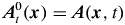 ${{\boldsymbol {A}}}^{0}_t({{ \boldsymbol {x} }})={{\boldsymbol {A}}}({{ \boldsymbol {x} }},t)$ in the notations of the previous section. Note, however, that the random process
 ${{\tilde {\boldsymbol {A}} }}^{s}_t({{ \boldsymbol {x} }})$ is not guaranteed to attain time
 $s=0$ before exiting from the domain. For any point
 ${{ \boldsymbol {x} }}\in \varOmega ,$ the stochastic particle trajectory
 ${{\tilde {{A}} }}^{s}_t({{ \boldsymbol {x} }})$ released at time
 $t$ first hits the boundary
 $\partial \varOmega$ at some finite, random time
 $s={{\tilde {\sigma }}}_t({{ \boldsymbol {x} }}) < t,$ evolving backward. The stochastic Lagrangian representations obtained by Constantin & Iyer (Reference Constantin and Iyer2011) for wall-bounded flows involve the ‘stopped process’
 ${{\tilde {\boldsymbol {A}} }}^{s\prime }_t({{ \boldsymbol {x} }}):={{\tilde {\boldsymbol {A}} }}^{s\vee {{\tilde {\sigma }}}_t({{ \boldsymbol {x} }})}_t({{ \boldsymbol {x} }}),$ which halts the stochastic Lagrangian particle as soon as it first hits the boundary, with the mathematical notation
 $s\vee {{\tilde {\sigma }}}_t({{ \boldsymbol {x} }}):=\max\{s,{{\tilde {\sigma }}}_t({{ \boldsymbol {x} }})\}.$ Since the realizations of
 ${{\tilde {\sigma }}}_t({{ \boldsymbol {x} }})$ are almost surely non-differentiable in
 ${{ \boldsymbol {x} }},$ we always take
 ${{\boldsymbol {\nabla }}}_x{{\tilde {\boldsymbol {A}} }}^{s\prime }_t({{ \boldsymbol {x} }}):={{\boldsymbol {\nabla }}}_x{{\tilde {\boldsymbol {A}} }}^{\sigma }_t({{ \boldsymbol {x} }})\big |_{\sigma =s\vee {{\tilde {\sigma }}}_t({{ \boldsymbol {x} }})}$ below.
With these notations, Constantin & Iyer (Reference Constantin and Iyer2011) in their Lemma 5.1 obtained the following stochastic Lagrangian representation of vortex momentum  ${{\boldsymbol {{p}}}}$ solving the viscous Kuz'min–Oseledets equation, with
 ${{\mathbb {E}}}$ denoting average over the random Brownian motions:
 \begin{equation} {{\boldsymbol{{p}}}}({{ \boldsymbol{x} }},t) ={{\mathbb{E}}}[ {{\boldsymbol{\nabla}}}_x{{\tilde{\boldsymbol{A}} }}^{0\prime}_t({{ \boldsymbol{x} }}) \boldsymbol{\cdot} {{\boldsymbol{{p}}}}_{dat}({{\tilde{\boldsymbol{A}} }}^{0\prime}_t({{ \boldsymbol{x} }}),0\vee{{\tilde{\sigma}}}_t({{ \boldsymbol{x} }}))]. \end{equation}
Here  ${{\boldsymbol {{p}}}}_{dat}$ represents the initial-boundary data, with
 ${{\boldsymbol {{p}}}}_{dat}({{ \boldsymbol {x} }},t)={{\boldsymbol {{p}}}}_0({{ \boldsymbol {x} }})$ for
 $t=0$ and
 ${{\boldsymbol {{p}}}}_{dat}({{ \boldsymbol {x} }},t)={{\boldsymbol {{p}}}}_W({{ \boldsymbol {x} }},t)$ for
 ${{ \boldsymbol {x} }}\in \partial \varOmega .$ Using the results of the previous subsection, the stochastic representation of the Navier–Stokes velocity stated in Theorem 3.1 of Constantin & Iyer (Reference Constantin and Iyer2011) follows as a simple corollary, i.e.
 \begin{align} {{\boldsymbol{u}}}({{ \boldsymbol{x} }},t) &= {{\mathbb{P}}}{{\mathbb{E}}}[ {{\boldsymbol{\nabla}}}_x{{\tilde{\boldsymbol{A}} }}^{0\prime}_t({{ \boldsymbol{x} }}) \boldsymbol{\cdot} {{\boldsymbol{{p}}}}_{dat} ({{\tilde{\boldsymbol{A}} }}^{0\prime}_t({{ \boldsymbol{x} }}),0\vee{{\tilde{\sigma}}}_t({{ \boldsymbol{x} }}))] \nonumber\\ &\quad = {{\mathbb{E}}}[ {{\boldsymbol{\nabla}}}_x{{\tilde{\boldsymbol{A}} }}^{0\prime}_t({{ \boldsymbol{x} }}) \boldsymbol{\cdot} {{\boldsymbol{{p}}}}_{dat} ({{\tilde{\boldsymbol{A}} }}^{0\prime}_t({{ \boldsymbol{x} }}),0\vee{{\tilde{\sigma}}}_t({{ \boldsymbol{x} }}))] -{{\boldsymbol{\nabla}}}\phi({{ \boldsymbol{x} }},t) \end{align}
with  ${{\boldsymbol {{p}}}}_{0}={{\boldsymbol {u}}}_0+{{\boldsymbol {\nabla }}}_x\phi _0$ at
 $t=0$ for any choice of
 $\phi _0$ and with
 ${{\boldsymbol {{p}}}}_{W}={{\boldsymbol {u}}}_W+{{\boldsymbol {\nabla }}}\phi$ at
 $\partial \varOmega ,$ where
 $\phi$ solves (2.27) for initial data
 $\phi _0$ and an arbitrary choice of b.c.
 $\phi _W$ on
 $\partial \varOmega .$ Constantin & Iyer (Reference Constantin and Iyer2011) used as initial data
 ${{\boldsymbol {{p}}}}_0={{\boldsymbol {u}}}_0$ only and also gave only an existence argument for suitable boundary data
 ${{\boldsymbol {{p}}}}_{W},$ but our use of the Kuz'min–Oseledets formalism provides a complete and explicit representation for the possible data. An interesting point is that this representation implies directly that
 $\hat {{\boldsymbol {n}}}\boldsymbol {\cdot }{{{\boldsymbol {\omega }}}}|_{\partial \varOmega }=0$ for motionless walls, since on the boundary
 $\hat {{\boldsymbol {n}}}\boldsymbol {\cdot }{{{\boldsymbol {\omega }}}}=(\hat {{\boldsymbol {n}}}\,{{{{\times }}}}\,{{\boldsymbol {\nabla }}}_x)\boldsymbol {\cdot }{{\boldsymbol {{p}}}}_{W}=(\hat {{\boldsymbol {n}}}\,{{{{\times }}}}\,{{\boldsymbol {\nabla }}}_x)\boldsymbol {\cdot } {{\boldsymbol {\nabla }}}_x\phi =0.$ Constantin & Iyer (Reference Constantin and Iyer2011) also provided in their Proposition 6.1 a stochastic Lagrangian representation of Navier–Stokes vorticity, i.e.
 \begin{equation} {{{\boldsymbol{\omega}}}}({{ \boldsymbol{x} }},t) ={{\mathbb{E}}}[ ({{\boldsymbol{\nabla}}}_x{{\tilde{\boldsymbol{A}} }}^{0\prime}_t({{ \boldsymbol{x} }}))^{\top\,-1} \boldsymbol{\cdot} {{{\boldsymbol{\omega}}}}_{dat}({{\tilde{\boldsymbol{A}} }}^{0\prime}_t({{ \boldsymbol{x} }}),0\vee{{\tilde{\sigma}}}_t({{ \boldsymbol{x} }}))], \end{equation}
with likewise  ${{{\boldsymbol {\omega }}}}_{dat}({{ \boldsymbol {x} }},t)={{{\boldsymbol {\omega }}}}_0({{ \boldsymbol {x} }})$ for
 $t=0$ and
 ${{{\boldsymbol {\omega }}}}_{dat}({{ \boldsymbol {x} }},t)={{{\boldsymbol {\omega }}}}_W({{ \boldsymbol {x} }},t)$ for
 ${{ \boldsymbol {x} }}\in \partial \varOmega .$ The boundary data
 ${{{\boldsymbol {\omega }}}}_W$ for the Navier–Stokes vorticity is not provided directly, of course, but only indirectly and non-locally by the stick b.c.
 ${{\boldsymbol {u}}}={{\boldsymbol {u}}}_W$ on the velocity field. In both (2.34) and (2.36) the solutions are represented by ensemble averages involving the initial and boundary data. However, in a flow entirely bounded by walls and asymptotically for very large
 $t$ the event
 ${{\tilde {\sigma }}}_t({{ \boldsymbol {x} }})>0$ holds with overwhelming probability, so that the solutions then depend almost entirely on the boundary data and almost not at all on the initial data.
We refer to the paper of Constantin & Iyer (Reference Constantin and Iyer2011) for detailed proofs of their Lemma 5.1 and Proposition 6.1. Here we give only very briefly the main idea of the argument. To prove Lemma 5.1, one obtains an evolution equation in  $s$ for
 ${{\boldsymbol {\nabla }}}_x{{\tilde {\boldsymbol {A}} }}^{s}_t({{ \boldsymbol {x} }}) \boldsymbol {\cdot } {{\boldsymbol {{p}}}}({{\tilde {\boldsymbol {A}} }}^{s}_t({{ \boldsymbol {x} }}),s)$ with
 ${{\boldsymbol {{p}}}}$ a given solution of the viscous Kuz'min–Oseledets equation (2.25a,b), starting at
 $s=t$ and integrating backward to
 $s=0\vee {{\tilde {\sigma }}}_t({{ \boldsymbol {x} }}).$ By taking the gradient of the stochastic ODE (2.33) for particle trajectories, one obtains
 \begin{equation} {\textrm{d}} ({{\boldsymbol{\nabla}}}_x{{\tilde{\boldsymbol{A}} }}^{s}_t) = ({{\boldsymbol{\nabla}}}_x{{\tilde{\boldsymbol{A}} }}^{s}_t) ({{\boldsymbol{\nabla}}}_x{{\boldsymbol{u}}})|_{({{\tilde{\boldsymbol{A}} }}^{s}_t,s)}{\textrm{d}}s , \quad s < t; \quad {{\boldsymbol{\nabla}}}_x{{\tilde{\boldsymbol{A}} }}^{t}_t={\boldsymbol{I}} , \end{equation}
which is now a deterministic ODE (along a stochastic trajectory) because the gradient of the Brownian motion vanishes. This ODE for the component column vectors  ${{\boldsymbol {\nabla }}}_x{{\tilde {a}}}^{s}_t({{ \boldsymbol {x} }})$,
 ${{\boldsymbol {\nabla }}}_x{{\tilde {b}}}^{s}_t({{ \boldsymbol {x} }})$,
 ${{\boldsymbol {\nabla }}}_x{{\tilde {c}}}^{s}_t({{ \boldsymbol {x} }})$ of
 ${{\boldsymbol {\nabla }}}_x{{\tilde {\boldsymbol {A}} }}^{s}_t$ closely resembles that describing Lie transport of a contravariant vector, except that it describes evolution along a stochastic trajectory
 $({{\tilde {\boldsymbol {A}} }}^{s}_t,s)$ backward in time
 $s<t$. On the other hand, using the backward Itō lemma and the fact that
 ${{\boldsymbol {{p}}}}$ solves the viscous Kuz'min–Oseledets equation (2.25a,b) gives
 \begin{align} \hat{{\textrm{d}}} {{\boldsymbol{{p}}}}({{\tilde{\boldsymbol{A}} }}^{s}_t,s) &= [D_s{{\boldsymbol{{p}}}}-\nu{{\varDelta}}_x{{\boldsymbol{{p}}}}]|_{({{\tilde{\boldsymbol{A}} }}^{s}_t,s)}\,{\textrm{d}}s + \sqrt{2\nu}\, \hat{{\textrm{d}}}{{\tilde{\textbf{W}}}}(s)\boldsymbol{\cdot}{{\boldsymbol{\nabla}}}){{\boldsymbol{{p}}}}|_{({{\tilde{\boldsymbol{A}} }}^{s}_t,s)} \nonumber\\ &= -({{\boldsymbol{\nabla}}}_x{{\boldsymbol{u}}}){{\boldsymbol{{p}}}}|_{({{\tilde{\boldsymbol{A}} }}^{s}_t,s)}\,{\textrm{d}}s + \sqrt{2\nu}\, \hat{{\textrm{d}}}{{\tilde{\textbf{W}}}}(s)\boldsymbol{\cdot}{{\boldsymbol{\nabla}}}){{\boldsymbol{{p}}}}|_{({{\tilde{\boldsymbol{A}} }}^{s}_t,s)}, \quad t>s>0\vee{{\tilde{\sigma}}}_t({{ \boldsymbol{x} }}) .\end{align}
Note that the backward Itō lemma supplies the viscous diffusion term  $-\nu {{\varDelta }}_x{{\boldsymbol {{p}}}}$ with the correct negative sign, whereas the more familiar forward Itō stochastic flow would yield instead
 $+\nu {{\varDelta }}_x{{\boldsymbol {{p}}}}$ with a positive sign. Equation (2.38) resembles that describing the Lie transport of a 1-form (covariant vector) but contains an additional random term from the Brownian motion. Combining (2.37) and (2.38) then leads to the final result:
 \begin{equation} \hat{{\textrm{d}}} [{{\boldsymbol{\nabla}}}_x{{\tilde{\boldsymbol{A}} }}^{s}_t \boldsymbol{\cdot} {{\boldsymbol{{p}}}}({{\tilde{\boldsymbol{A}} }}^{s}_t,s)] =\sqrt{2\nu}\, ({{\boldsymbol{\nabla}}}_x{{\tilde{\boldsymbol{A}} }}^{s}_t)\, (\hat{{\textrm{d}}}{{\tilde{\textbf{W}}}}(s)\boldsymbol{\cdot}{{\boldsymbol{\nabla}}}) {{\boldsymbol{{p}}}}|_{({{\tilde{\boldsymbol{A}} }}^{s}_t,s)}, \quad t>s>0\vee{{\tilde{\sigma}}}_t({{ \boldsymbol{x} }}). \end{equation}
This yields the representation of Lemma 5.1, because the final surviving term on the right-hand side is a backward martingale with zero average. In fact, we obtain the even stronger result that  ${{\boldsymbol {\nabla }}}_x{{\tilde {\boldsymbol {A}} }}^{s}_t({{ \boldsymbol {x} }}) \boldsymbol {\cdot } {{\boldsymbol {{p}}}}({{\tilde {\boldsymbol {A}} }}^{s}_t({{ \boldsymbol {x} }}),s)$ is a backward martingale, which is thus stochastically conserved and whose (deterministic) value
 ${{\boldsymbol {{p}}}}({{ \boldsymbol {x} }},t)$ at
 $s=t$ is equal to its average value at
 $s=0\vee {{\tilde {\sigma }}}_t({{ \boldsymbol {x} }}).$
In the same manner for any solution  ${{{\boldsymbol {\omega }}}}$ of the viscous Helmholtz equation (2.32) one has the backward martingale evolving as
 \begin{align} \hat{{\textrm{d}}}[({{\boldsymbol{\nabla}}}_x{{\tilde{\boldsymbol{A}} }}^{s}_t)^{\top\,-1} \boldsymbol{\cdot} {{{\boldsymbol{\omega}}}}({{\tilde{\boldsymbol{A}} }}^{s}_t,s)] =\sqrt{2\nu}\, ({{\boldsymbol{\nabla}}}_x{{\tilde{\boldsymbol{A}} }}^{s}_t)^{\top\, -1} \, (\hat{{\textrm{d}}}{{\tilde{\textbf{W}}}}(s)\boldsymbol{\cdot}{{\boldsymbol{\nabla}}}){{{\boldsymbol{\omega}}}}|_{({{\tilde{\boldsymbol{A}} }}^{s}_t,s)} \quad t>s>0\vee{{\tilde{\sigma}}}_t({{ \boldsymbol{x} }}) , \end{align}
and this yields the representation for vorticity in Proposition 6.1. The derivation of (2.40) is very similar to that given for (2.39). First, it follows immediately from (2.37) that
 \begin{align} {\textrm{d}} ({{\boldsymbol{\nabla}}}_x{{\tilde{\boldsymbol{A}} }}^{s}_t({{ \boldsymbol{x} }}))^{{-}1\top} = -({{\boldsymbol{\nabla}}}_x{{\tilde{\boldsymbol{A}} }}^{s}_t({{ \boldsymbol{x} }}))^{{-}1\top} \boldsymbol{\cdot} ({{\boldsymbol{\nabla}}}_x{{\boldsymbol{u}}})^{\top}|_{({{\tilde{\boldsymbol{A}} }}^{s}_t,s)}\,{\textrm{d}}s , \quad s < t; \quad ({{\boldsymbol{\nabla}}}_x{{\tilde{\boldsymbol{A}} }}^{t}_t({{ \boldsymbol{x} }}))^{{-}1\top}={\boldsymbol{I}} . \end{align}
Component row vectors of 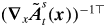 $({{\boldsymbol {\nabla }}}_x{{\tilde {\boldsymbol {A}} }}^{s}_t({{ \boldsymbol {x} }}))^{-1\top }$ represent
 $({{\boldsymbol {\nabla }}}_a{\tilde x}^{s}_t({{\boldsymbol {a}}}))^{\top },$
 $({{\boldsymbol {\nabla }}}_a{\tilde y}^{s}_t({{\boldsymbol {a}}}))^{\top },$
 $({{\boldsymbol {\nabla }}}_a{\tilde z}^{s}_t({{\boldsymbol {a}}}))^{\top }$ and (2.41) describes their quasi-Lie-transport as 1-forms (covariant derivatives). On the other hand, from the backward Itō lemma and the Helmholtz equation
 \begin{align} \hat{{\textrm{d}}} {{{\boldsymbol{\omega}}}}({{\tilde{\boldsymbol{A}} }}^{s}_t,s) &= [D_s{{{\boldsymbol{\omega}}}}-\nu{{\varDelta}}_x{{{\boldsymbol{\omega}}}}]|_{({{\tilde{\boldsymbol{A}} }}^{s}_t,s)}\,{\textrm{d}}s + \sqrt{2\nu}\, (\hat{{\textrm{d}}}{{\tilde{\textbf{W}}}}(s)\boldsymbol{\cdot}{{\boldsymbol{\nabla}}}){{{\boldsymbol{\omega}}}}|_{({{\tilde{\boldsymbol{A}} }}^{s}_t,s)} \nonumber\\ &=({{{\boldsymbol{\omega}}}}\boldsymbol{\cdot}{{\boldsymbol{\nabla}}}_x){{\boldsymbol{u}}}|_{({{\tilde{\boldsymbol{A}} }}^{s}_t,s)}\,{\textrm{d}}s + \sqrt{2\nu}\, (\hat{{\textrm{d}}}{{\tilde{\textbf{W}}}}(s)\boldsymbol{\cdot}{{\boldsymbol{\nabla}}}){{{\boldsymbol{\omega}}}}|_{({{\tilde{\boldsymbol{A}} }}^{s}_t,s)}, \quad t>s>0\vee{{\tilde{\sigma}}}_t({{ \boldsymbol{x} }}). \end{align}
Except for the new stochastic term from the Brownian motion, this equation describes quasi-Lie-transport of the vorticity as a covariant vector (the Hodge dual of the vorticity 2-form  $(\partial _i u_j-\partial _j u_i)\,\textrm{d}x^{i} \,\textrm{d}x^{j}$). Combining (2.41) and (2.42) yields the result (2.40).
The intuitive meaning of these formulae becomes more clear if one integrates along stochastic trajectories  ${{\tilde {\boldsymbol {A}} }}^{\tau }_t({{ \boldsymbol {x} }})$ forward in time from
 $\tau =0\vee {{\tilde {\sigma }}}_t({{ \boldsymbol {x} }})$ to
 $\tau =t,$ rather than backward in time. Note that an explicit solution for
 ${{\boldsymbol {\nabla }}}_x{{\tilde {\boldsymbol {A}} }}^{s}_t$ is given by the time-ordered matrix exponential, with matrix products ordered right to left for increasing time:
 \begin{equation} {{\boldsymbol{\nabla}}}_x{{\tilde{\boldsymbol{A}} }}^{s}_t = T\,\textrm{exp}\left[-\int_s^{t}\textrm{d}r\,\left.({{\boldsymbol{\nabla}}}_x{{\boldsymbol{u}}})\right|_{({{\tilde{\boldsymbol{A}} }}^{r}_t,r)}\right]. \end{equation}
If one defines starting values in terms of the randomly sampled initial-boundary data
 \begin{equation} \tilde{{{\boldsymbol{{p}}}}}({{ \boldsymbol{x} }},0\vee{{\tilde{\sigma}}}_t({{ \boldsymbol{x} }})) := {{\boldsymbol{{p}}}}_{dat}({{\tilde{\boldsymbol{A}} }}^{0\prime}_t({{ \boldsymbol{x} }}),0\vee{{\tilde{\sigma}}}_t({{ \boldsymbol{x} }})), \end{equation}
and defines at later times
 \begin{equation} \tilde{{{\boldsymbol{{p}}}}}({{ \boldsymbol{x} }},\tau) := T\,\textrm{exp}\left[-\int_{0\vee{{\tilde{\sigma}}}_t({{ \boldsymbol{x} }})}^{\tau} \textrm{d}r\, \left.({{\boldsymbol{\nabla}}}_x{{\boldsymbol{u}}})\right|_{({{\tilde{\boldsymbol{A}} }}^{r}_t,r)}\right] \tilde{{{\boldsymbol{{p}}}}}({{ \boldsymbol{x} }},0\vee{{\tilde{\sigma}}}_t({{ \boldsymbol{x} }})), \quad t>\tau > 0\vee{{\tilde{\sigma}}}_t({{ \boldsymbol{x} }}), \end{equation}
then the stochastic representation in Lemma 5.1 can be expressed simply as
 \begin{equation} {{\boldsymbol{{p}}}}({{ \boldsymbol{x} }},t) = {{\mathbb{E}}}[\tilde{{{\boldsymbol{{p}}}}}({{ \boldsymbol{x} }},t)]. \end{equation}
However, by direct differentiation of the matrix exponential in (2.45), one can see that
 \begin{equation} \frac{\textrm{d}}{\textrm{d}\tau} \tilde{{{\boldsymbol{{p}}}}}({{ \boldsymbol{x} }},\tau) ={-}\left. ({{\boldsymbol{\nabla}}}_x{{\boldsymbol{u}}})\right|_{({{\tilde{\boldsymbol{A}} }}^{\tau}_t,\tau)} \tilde{{{\boldsymbol{{p}}}}}({{ \boldsymbol{x} }},\tau), \quad t>\tau > 0\vee{{\tilde{\sigma}}}_t({{ \boldsymbol{x} }}). \end{equation}
This appears exactly the same as the Lie-transport equation of a 1-form except that the material derivative  $D_\tau$ has been replaced with the time derivative
 $\partial /\partial \tau$ along the random trajectory
 ${{\tilde {\boldsymbol {A}} }}^{\tau }_t({{ \boldsymbol {x} }})$ starting at
 $\tau = 0\vee {{\tilde {\sigma }}}_t({{ \boldsymbol {x} }})$ and ending at
 $\tau =t.$ We thus see that the randomly sampled initial-boundary data
 $\tilde {{{\boldsymbol {{p}}}}}(0\vee {{\tilde {\sigma }}}_t({{ \boldsymbol {x} }}))$ is quasi-Lie-transported as a 1-form along stochastic trajectories forward in time to point
 $({{ \boldsymbol {x} }},t)$ and the resulting contributions
 $\tilde {{{\boldsymbol {{p}}}}}({{ \boldsymbol {x} }},t)$ are averaged over the ensemble to yield
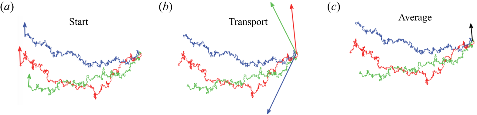
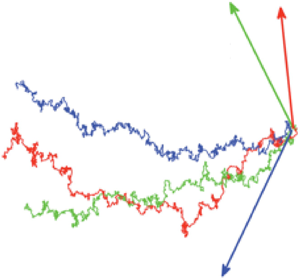
 ${{\boldsymbol {{p}}}}({{ \boldsymbol {x} }},t).$ The process is illustrated in figure 1. In this stochastic Lagrangian representation, the quasi-Lie-transport along stochastic trajectories represents the nonlinear dynamics of vortex momentum under the Kuz'min–Oseledets equation and cancellations in the ensemble average represent the destruction of vortex momentum by viscosity. The analogous interpretation holds for the vorticity representation in Proposition 6.1. Using the similar matrix exponential
 \begin{equation} ({{\boldsymbol{\nabla}}}_x{{\tilde{\boldsymbol{A}} }}^{s}_t)^{\top\,-1} = T\,\textrm{exp}\left[ \int_s^{t} \textrm{d}r\left.({{\boldsymbol{\nabla}}}_x{{\boldsymbol{u}}})^{\top}\right|_{({{\tilde{\boldsymbol{A}} }}^{r}_t,r)}\right], \end{equation}
one can show that randomly sampled initial-boundary data
 \begin{equation} \tilde{{{{\boldsymbol{\omega}}}}}({{ \boldsymbol{x} }},0\vee{{\tilde{\sigma}}}_t({{ \boldsymbol{x} }}) ) = {{{\boldsymbol{\omega}}}}_{dat}({{\tilde{\boldsymbol{A}} }}^{0\prime}_t({{ \boldsymbol{x} }}),0\vee{{\tilde{\sigma}}}_t({{ \boldsymbol{x} }})) \end{equation}
are quasi-Lie-transported along stochastic trajectories  ${{\tilde {\boldsymbol {A}} }}^{\tau }_t({{ \boldsymbol {x} }})$ from
 $\tau = 0\vee {{\tilde {\sigma }}}_t({{ \boldsymbol {x} }})$ to
 $\tau =t$ according to the equation
 \begin{equation} \frac{\textrm{d}}{\textrm{d}\tau} \tilde{{{{\boldsymbol{\omega}}}}}({{ \boldsymbol{x} }},\tau) = \left. (\tilde{{{{\boldsymbol{\omega}}}}}({{ \boldsymbol{x} }},\tau)\boldsymbol{\cdot}{{\boldsymbol{\nabla}}}_x){{\boldsymbol{u}}} \right|_{({{\tilde{\boldsymbol{A}} }}^{\tau}_t,\tau)}, \quad t>\tau > 0\vee{{\tilde{\sigma}}}_t({{ \boldsymbol{x} }}), \end{equation}
which closely resembles the usual inviscid evolution equation for vorticity. The final contributions at  $\tau =t$ are then averaged over the ensemble to give the resultant vorticity
 \begin{equation} {{{\boldsymbol{\omega}}}}({{ \boldsymbol{x} }},t) = {{\mathbb{E}}}[\tilde{{{{\boldsymbol{\omega}}}}}({{ \boldsymbol{x} }},t)], \end{equation}
and cancellations in this average over random contributions represent the viscous destruction of vorticity in a Lagrangian framework.
Illustration of the stochastic representation, with three sample realizations shown in blue, red and green. (a) Input vectors at time  $\tau =0\vee {{\tilde {\sigma }}}_t({{ \boldsymbol {x} }})$ are sampled at random locations by stochastic Lagrangian trajectories going backward in time
 $\tau$ from space–time point
 $({{ \boldsymbol {x} }},t)$. (b) The vectors are Lie transported along the stochastic trajectories forward in time from
 $\tau =0\vee {{\tilde {\sigma }}}_t({{ \boldsymbol {x} }})$ to
 $\tau =t,$ when the vectors arrive to point
 ${{ \boldsymbol {x} }}$ stretched and rotated by the flow. (c) The random vectors at
 $({{ \boldsymbol {x} }},t)$ are ensemble averaged to obtain the resultant vector.

Although the physical interpretation is made more transparent by integrating forward in time, the method of proof integrating backward in time yields a more powerful result. It is obviously an arbitrary decision to make  $0$ the ‘initial time’ and one can instead solve the viscous Kuz'min–Oseledets and Helmholtz equations starting at any time
 $s < t$ with initial data
 ${{\boldsymbol {{p}}}}(\boldsymbol {\cdot },s).$ In that case, the same arguments as for
 $s=0$ yield
 \begin{equation} {{\boldsymbol{{p}}}}({{ \boldsymbol{x} }},t) = {{\mathbb{E}}}[ \tilde{{{\boldsymbol{{p}}}}}_s({{ \boldsymbol{x} }},t)] , \quad s < t \end{equation}
with
 \begin{equation} \tilde{{{\boldsymbol{{p}}}}}_s({{ \boldsymbol{x} }},t) := {{\boldsymbol{\nabla}}}_x{{\tilde{\boldsymbol{A}} }}^{s\prime}_t({{ \boldsymbol{x} }}) \boldsymbol{\cdot} {{\boldsymbol{{p}}}}({{\tilde{\boldsymbol{A}} }}^{s\prime}_t({{ \boldsymbol{x} }}),s\vee{{\tilde{\sigma}}}_t({{ \boldsymbol{x} }})), \end{equation}
and likewise
 \begin{equation} {{{\boldsymbol{\omega}}}}({{ \boldsymbol{x} }},t) ={{\mathbb{E}}}[\tilde{{{{\boldsymbol{\omega}}}}}_s({{ \boldsymbol{x} }},t)], \quad s < t \end{equation}
with
 \begin{equation} \tilde{{{{\boldsymbol{\omega}}}}}_s({{ \boldsymbol{x} }},t):=({{\boldsymbol{\nabla}}}_x{{\tilde{\boldsymbol{A}} }}^{s\prime}_t({{ \boldsymbol{x} }}))^{\top\,-1} \boldsymbol{\cdot} {{{\boldsymbol{\omega}}}}({{\tilde{\boldsymbol{A}} }}^{s\prime}_t({{ \boldsymbol{x} }}),s\vee{{\tilde{\sigma}}}_t({{ \boldsymbol{x} }})). \end{equation}
The quantities  $\tilde {{{\boldsymbol {{p}}}}}_s({{ \boldsymbol {x} }},t)$ and
 $\tilde {{{{\boldsymbol {\omega }}}}}_s({{ \boldsymbol {x} }},t)$ defined above are the backward martingale random processes in
 $s$ that were used in the proofs of Lemma 5.1 and Proposition 6.1, which are thus statistically conserved for every choice of
 ${{ \boldsymbol {x} }}\in \varOmega .$ If
 $s=0$ then
 $\tilde {{{\boldsymbol {{p}}}}}_0({{ \boldsymbol {x} }},t),$
 $\tilde {{{{\boldsymbol {\omega }}}}}_0({{ \boldsymbol {x} }},t)$ are the same quantities
 $\tilde {{{\boldsymbol {{p}}}}}({{ \boldsymbol {x} }},t),$
 $\tilde {{{{\boldsymbol {\omega }}}}}({{ \boldsymbol {x} }},t)$ that were introduced in discussing the physical interpretation using forward integration. The proofs in Constantin & Iyer (Reference Constantin and Iyer2011) thus provide an infinite set of stochastic Lagrangian conservation laws for incompressible Navier–Stokes solutions. We shall refer to
 $\tilde {{{{\boldsymbol {\omega }}}}}_s({{ \boldsymbol {x} }},t)$ for
 ${{ \boldsymbol {x} }}\in \varOmega$ and
 $s<t,$ in particular, as the stochastic Cauchy invariants, since they generalize the Cauchy vorticity invariants of incompressible Euler solutions. See Frisch & Villone (Reference Frisch and Villone2014) for historical perspective. One fundamental difference is that the Cauchy invariants for Euler are conserved both forward and backward in time, but the stochastic Cauchy invariants for Navier–Stokes are conserved only backward in time. This difference arises because the Navier–Stokes equation, unlike Euler, is time irreversible and the stochastic Cauchy invariants express the fixed arrow of time. For this same reason, we have written the stochastic invariants as functions of the particle position ‘labels’
 ${{ \boldsymbol {x} }}$ at the final time
 $t$ rather than, as usual for ideal fluids, in terms of the particle positions
 ${{\boldsymbol {a}}}$ at early times
 $s<t.$ As we shall see in the discussion of numerical methods in the next section, realizations of
 $\tilde {{{\boldsymbol {{p}}}}}_s({{ \boldsymbol {x} }},t)$,
 $\tilde {{{{\boldsymbol {\omega }}}}}_s({{ \boldsymbol {x} }},t)$ can be calculated for all
 $s<t$ by a simple integration scheme backward in time using ensembles of stochastic Lagrangian particles. The requirement that their average values remain independent of
 $s$ is a stringent test on the accuracy of the numerics.
2.3. Relation with the Lighthill–Morton theory
The Constantin & Iyer (Reference Constantin and Iyer2011) representation (2.54), (2.55) for any flow entirely bounded by walls allows one to reconstruct the interior vorticity  ${{{\boldsymbol {\omega }}}}({{ \boldsymbol {x} }},t)$ at any point
 ${{ \boldsymbol {x} }}\in \varOmega$ and time
 $t$ in terms of the vorticity at the boundary, by taking the time interval
 $t-s$ so large that
 ${{\tilde {\sigma }}}_t({{ \boldsymbol {x} }})>s$ with overwhelming probability. This formula thus makes very concrete the truism that all vorticity in the flow originates, ultimately, at a solid wall. The Constantin & Iyer (Reference Constantin and Iyer2011) theory does not address the generation of the wall vorticity, but instead takes the boundary values
 ${{{\boldsymbol {\omega }}}}_W({{ \boldsymbol {x} }},t)$ for
 ${{ \boldsymbol {x} }}\in \partial \varOmega$ as a given. It therefore plays a rather complementary role to the theory of Lighthill (Reference Lighthill and Rosenhead1963) and Morton (Reference Morton1984), which was advanced to explain the inviscid generation of vorticity at the wall. The Constantin & Iyer (Reference Constantin and Iyer2011) formulae instead describe, in a Lagrangian framework, the subsequent transport of vorticity away from the walls by nonlinear advection, stretching and viscous diffusion. In order to discuss more clearly the relations of the two approaches, we must first review briefly the Lighthill–Morton theory, especially since some minor controversies still exist regarding its general formulation.
The concept of ‘vorticity source’ or ‘vorticity flux density’ was first introduced in the pioneering work of Lighthill (Reference Lighthill and Rosenhead1963), who identified vorticity generation in an infinitesimal layer at a solid, stationary wall as an essentially inviscid process driven by tangential pressure gradients. Lighthill's theory was extended by Morton (Reference Morton1984) to accelerating walls, with the conclusion that the source of tangential vorticity at the wall is given by
 \begin{equation} {{{\boldsymbol{\sigma}}}} = \left. \hat{{\boldsymbol{n}}}\times ({{\boldsymbol{\nabla}}}_xp + D_t{{\boldsymbol{u}}}) \right|_{\partial\varOmega} , \end{equation}
at least for a flow domain with a two-dimensional flat boundary and constant outward unit normal vector, say,  $\hat {{\boldsymbol {n}}}=-\hat {{\boldsymbol {y}}}$. This quantity has dimensions of
 $(\textrm {vorticity})\times (\textrm {velocity})$. Concretely, by the Kelvin theorem,
 ${{{\boldsymbol {\sigma }}}}\boldsymbol {\cdot } \hat {{\boldsymbol {n}}}\times \textrm {d}{\boldsymbol {l}}$ represents the rate of generation of circulation along a small line element
 $\textrm {d}{\boldsymbol {l}}=\hat {{\boldsymbol {t}}} \,\textrm {{d}}s,$ with
 $\hat {{\boldsymbol {t}}}$ any unit vector tangent to the wall, and, thus,
 ${{{\boldsymbol {\sigma }}}}\boldsymbol {\cdot } \hat {{\boldsymbol {n}}}\,{{{{\times }}}}\,\hat {{\boldsymbol {t}}}$ represents the wall-normal flux of vorticity generated in the direction
 $\hat {{\boldsymbol {n}}}\,{{{{\times }}}}\,\hat {{\boldsymbol {t}}}$ (Morton Reference Morton1984; Eyink Reference Eyink2008). Applying the momentum-balance (Navier–Stokes) equations at the wall, for the simplified two-dimensional geometry, Lighthill (Reference Lighthill and Rosenhead1963) and Morton (Reference Morton1984) obtained alternative expressions for the tangential vorticity source:
 \begin{equation} \sigma_x = \left.-\nu \frac{\partial\omega_x}{\partial y}\right|_{\partial\varOmega}, \quad \sigma_z = \left.-\nu \frac{\partial\omega_z}{\partial y}\right|_{\partial\varOmega}. \end{equation}
These formulae express the instantaneous balance between the rate of generation of vorticity at the wall and the rate of viscous diffusion of vorticity away from the wall. Using the facts that  $\partial \omega _y/\partial x|_{\partial \varOmega }=0$ and
 $\partial \omega _y/\partial z|_{\partial \varOmega }=0,$ the latter expressions can be rewritten as
 \begin{equation} {{{\boldsymbol{\sigma}}}} ={-}\nu \hat{{\boldsymbol{n}}}\times ({{\boldsymbol{\nabla}}}_x\times{{{\boldsymbol{\omega}}}}) |_{\partial\varOmega} = {{\boldsymbol{\Sigma}}}\hat{{\boldsymbol{n}}}|_{\partial\varOmega}, \end{equation}
where  ${{\boldsymbol {\Sigma }}}$ is the vorticity flux for Navier–Stokes defined in (1.2a,b) as an anti-symmetric matrix. Since
 $-{{\boldsymbol {\Sigma }}}^{\top }\hat {{\boldsymbol {n}}}$ represents generally the flux of vector vorticity in the space direction
 $-\hat {{\boldsymbol {n}}}$ (inward unit normal), (2.58) has a natural physical interpretation and plausibly generalizes the Lighthill–Morton theory to flow domains with three-dimensional, curvilinear boundaries. This generalization was first proposed by Lyman (Reference Lyman1990).
There is a subtlety, however, because the concept of a ‘vorticity flux vector’ is only defined up to a divergence-free contribution, and the most standard choice of viscous flux is not the anti-symmetric tensor in (1.2a,b) but is instead  ${{\boldsymbol {\Sigma }}}'_{visc} =-\nu {{\boldsymbol {\nabla }}}_x{{{\boldsymbol {\omega }}}}.$ This yields
 \begin{equation} {{{\boldsymbol{\sigma}}}}' = \left.-{{\boldsymbol{\Sigma}}}^{\prime \top} \hat{{\boldsymbol{n}}}\right|_{\partial\varOmega} = \left.\nu (\hat{{\boldsymbol{n}}}\boldsymbol{\cdot}{{\boldsymbol{\nabla}}}_x){{{\boldsymbol{\omega}}}} \right|_{\partial\varOmega}, \end{equation}
which was suggested already by Panton (Reference Panton1984, §§ 13.7, 13.11) and still often espoused (Wu & Wu Reference Wu and Wu1993, Reference Wu and Wu1996, Reference Wu and Wu1998). There are obvious distinctions between the two proposals. In particular,  ${{\boldsymbol {\Sigma }}}$ is anti-symmetric, so that
 ${{{\boldsymbol {\sigma }}}}\boldsymbol {\cdot }\hat {{\boldsymbol {n}}}=0$ and, thus, Lyman's generalization predicts no generation of vorticity normal to the boundary. However, even for a flat, two-dimensional wall, typically
 ${{{\boldsymbol {\sigma }}}}'\boldsymbol {\cdot }\hat {{\boldsymbol {n}}}\neq 0.$ The latter result seems implausible, since wall-normal vorticity is associated to flux through loops lying entirely within the wall and pressure gradients can drive no net circulation round such loops. However, we believe that a stronger argument in favour of
 ${{{\boldsymbol {\sigma }}}}$ rather than
 ${{{\boldsymbol {\sigma }}}}'$, is that it is
 ${{\boldsymbol {\Sigma }}}$ which appears in the momentum balance (1.1) and not
 ${{\boldsymbol {\Sigma }}}'.$ Thus, it is only (2.58) which corresponds to the Lighthill–Morton inviscid expression (2.56) for a general three-dimensional boundary, and the Kelvin theorem argument of Morton (Reference Morton1984) and Eyink (Reference Eyink2008) then gives a spatially local meaning to
 ${{{\boldsymbol {\sigma }}}}.$ For this reason, we shall here adopt (2.56) and (2.58) as the generally correct formulation. Fortunately, there is no difference in the predictions of the competing proposals of Lyman (Reference Lyman1990) and Panton (Reference Panton1984) for the example which is studied numerically in this work, namely, the flux of tangential vorticity away from a flat, two-dimensional channel wall, so we may disregard this issue hereafter.
The Lighthill–Morton theory is directly related to the statistical result (1.4) derived by Taylor (Reference Taylor1932) and Huggins (Reference Huggins1994) for statistically stationary turbulence in domains with non-accelerating walls, i.e.
 \begin{equation} \bar{\Sigma}_{ij} = \epsilon_{ijk} \partial_k \overline{\left( p+\tfrac{1}{2}|{{\boldsymbol{u}}}|^{2}\right)}, \end{equation}
which locally relates vorticity flux and generalized pressure gradients at interior points. The time-averaged tangential vorticity source relation of Lighthill–Morton,
 \begin{equation} \bar{\sigma}_i =\left.\bar{\Sigma}_{ij}\hat{n}_j\right|_{\partial\varOmega} = \left.(\hat{{\boldsymbol{n}}}\times{{\boldsymbol{\nabla}}}_x \bar{p})_i \right|_{\partial\varOmega}, \end{equation}
is just the Taylor–Huggins relation (2.60) approaching a boundary point and considering the wall-normal flux of vorticity driven by mean tangential pressure gradients. Here we note that there may be an average transport of tangential vorticity also parallel to the wall, driven by mean wall-normal gradients of generalized pressure:
 \begin{equation} \frac{\partial}{\partial n} \left.\overline{p+(1/2)|{{\boldsymbol{u}}}|^{2}}\right|_{\partial\varOmega} = \frac{1}{2} \left.\epsilon_{ijk} \hat{n}_i \bar{\Sigma}_{jk}\right|_{\partial\varOmega} =\left.-\nu(\hat{{\boldsymbol{n}}}\times{{\boldsymbol{\nabla}}}_x)\boldsymbol{\cdot}\bar{{{{\boldsymbol{\omega}}}}}\right|_{\partial\varOmega}. \end{equation}
The above relation is just the time average of the standard Neumann boundary condition on the pressure (noting that  $(\partial /\partial n)|{{\boldsymbol {u}}}|^{2}=0$ at the wall). The Taylor–Huggins result (2.60) continues both of the time-averaged relations (2.61) and (2.62) into the interior of the flow, where the vorticity current tensor in (1.2a,b) for an incompressible Navier–Stokes fluid takes the form
 \begin{equation} \Sigma_{ij} = u_i\omega_j - u_j\omega_i + \nu\left(\frac{\partial\omega_i}{\partial x_j}- \frac{\partial\omega_j}{\partial x_i}\right), \end{equation}
with contributions not only from viscous diffusion but also from nonlinear advection and stretching by the fluid flow velocity.
The Constantin–Iyer formalism provides a Lagrangian description of the space transport of vorticity, with contributions from the same physical processes that are represented by the Eulerian vorticity current (2.63). The stochastic Cauchy invariant (2.55) can be directly related to the vorticity current by integration over any open subdomain  $O\subset \varOmega$ with smooth boundary
 $\partial O$ and by statistical expectation, yielding
 \begin{equation} {{\mathbb{E}}}\left[\int_O \textrm{d}^{3}x\left(\tilde{{{{\boldsymbol{\omega}}}}}_s({{ \boldsymbol{x} }},t) - {{{\boldsymbol{\omega}}}}({{ \boldsymbol{x} }},s) \right) \right] = \int_s^{t} \textrm{d}r \int_{\partial O} {{\boldsymbol{\Sigma}}}({{ \boldsymbol{x} }},r)\boldsymbol{\cdot} \textrm{d}\,{\boldsymbol{A}}, \quad s < t, \end{equation}
where  $\textrm {d}\,{{\boldsymbol {A}}}$ is the outward-pointing vector area element on
 $\partial O$. Of course, here
 ${{\boldsymbol {\Sigma }}}$ and
 ${{\boldsymbol {\Sigma }}}'$ yield the same total surface integral, as does any other vorticity current that differs from these two by a divergence-free vector. Detailed understanding of the physical processes contributing in the Constantin–Iyer representation can be obtained by decomposing
 \begin{equation} (\tilde{{{{\boldsymbol{\omega}}}}}_s({{ \boldsymbol{x} }},t) - {{{\boldsymbol{\omega}}}}({{ \boldsymbol{x} }},s) ) = ({{{\boldsymbol{\omega}}}}({{\tilde{\boldsymbol{A}} }}^{s}_t({{ \boldsymbol{x} }}),s)-{{{\boldsymbol{\omega}}}}({{ \boldsymbol{x} }},s)) + (\tilde{{{{\boldsymbol{\omega}}}}}_s({{ \boldsymbol{x} }},t) -{{{\boldsymbol{\omega}}}}({{\tilde{\boldsymbol{A}} }}^{s}_t({{ \boldsymbol{x} }}),s)). \end{equation}
The first term on the right-hand side of (2.65) represents spatial transport of vorticity by fluid advection and viscous diffusion, while the second term represents space transport by vortex stretching. To see this, note that the space integral of the first term gives
 \begin{equation} \int_O \textrm{d}^{3}x({{{\boldsymbol{\omega}}}}({{\tilde{\boldsymbol{A}} }}^{s}_t({{ \boldsymbol{x} }}),s)-{{{\boldsymbol{\omega}}}}({{ \boldsymbol{x} }},s)) =\int_{{{\tilde{\boldsymbol{A}} }}^{s}_t(O)\backslash O} \textrm{d}^{3}x\,{{{\boldsymbol{\omega}}}}({{ \boldsymbol{x} }},s) - \int_{O\backslash {{\tilde{\boldsymbol{A}} }}^{s}_t(O)} \textrm{d}^{3}x\,{{{\boldsymbol{\omega}}}}({{ \boldsymbol{x} }},s) \end{equation}
for  $t>s>{{\tilde {\sigma }}}_t(O):=\sup _{{{ \boldsymbol {x} }}\in O} {{\tilde {\sigma }}}_t({{ \boldsymbol {x} }}),$ because the stochastic flow preserves the volume elements in
 $O$ before any particle hits the flow boundary. The expression on the right-hand side of (2.66) transparently represents change of the space integral by transport due to advection and viscous diffusion. Indeed, the integration set
 ${{\tilde {\boldsymbol {A}} }}^{s}_t(O)\backslash O$ consists of points outside
 $O$ at time
 $s$ that enter it by time
 $t$ and their contribution has a positive sign, whereas the set
 $O\backslash {{\tilde {\boldsymbol {A}} }}^{s}_t(O)$ consists of points inside
 $O$ at time
 $s$ that leave it by time
 $t$ and their contribution has a negative sign. Note furthermore from Constantin & Iyer (Reference Constantin and Iyer2011), Proposition 5.2 that
 \begin{align} \lim_{s\to t-} \frac{1}{t-s} {{\mathbb{E}}}[ {{{\boldsymbol{\omega}}}}({{\tilde{\boldsymbol{A}} }}^{s}_t({{ \boldsymbol{x} }}),s)-{{{\boldsymbol{\omega}}}}({{ \boldsymbol{x} }},s)] &={-}({{\boldsymbol{u}}}({{ \boldsymbol{x} }},t)\boldsymbol{\cdot}{{\boldsymbol{\nabla}}}){{{\boldsymbol{\omega}}}}({{ \boldsymbol{x} }},t) + \nu{\rm \Delta}{{{\boldsymbol{\omega}}}}({{ \boldsymbol{x} }},t) \nonumber\\ &={-}{{\boldsymbol{\nabla}}}\boldsymbol{\cdot} \left[{{\boldsymbol{u}}}{{{\boldsymbol{\omega}}}} +{{\boldsymbol{\Sigma}}}_{visc} \right], \end{align}
with  ${{\boldsymbol {\Sigma }}}_{visc} = - \nu [({{\boldsymbol {\nabla }}}{{{\boldsymbol {\omega }}}})-({{\boldsymbol {\nabla }}}{{{\boldsymbol {\omega }}}})^{\top }]$. The first term in (2.65) thus recovers the instantaneous contributions to
 ${{\boldsymbol {\Sigma }}}$ from advection and viscous diffusion in the limit
 $s\to t-.$ On the other hand, the second term in (2.65) can be rewritten using the definition (2.55) of the stochastic Cauchy invariant, as
 \begin{equation} (\tilde{{{{\boldsymbol{\omega}}}}}_s({{ \boldsymbol{x} }},t) -{{{\boldsymbol{\omega}}}}({{\tilde{\boldsymbol{A}} }}^{s}_t({{ \boldsymbol{x} }}),s)) = [({{\boldsymbol{\nabla}}}_x{{\tilde{\boldsymbol{A}} }}^{s}_t({{ \boldsymbol{x} }}))^{\top\,-1} -{\boldsymbol{I}}] \boldsymbol{\cdot} {{{\boldsymbol{\omega}}}}({{\tilde{\boldsymbol{A}} }}^{s}_t({{ \boldsymbol{x} }}),s) \end{equation}
for  $t>s>{{\tilde {\sigma }}}_t({{ \boldsymbol {x} }}).$ The vector
 ${{{\boldsymbol {\omega }}}}({{\tilde {\boldsymbol {A}} }}^{s}_t({{ \boldsymbol {x} }}),s)$ represents the initial vorticity sampled at time
 $s,$ while the matrix
 $({{\boldsymbol {\nabla }}}_x{{\tilde {\boldsymbol {A}} }}^{s}_t({{ \boldsymbol {x} }}))^{\top \,-1} -{\boldsymbol {I}}$ represents the accumulated change from stretching and rotation between times
 $s$ and
 $t,$ as illustrated by the middle panel of figure 1. Note that it follows either from the equation of motion (2.37) for
 ${{\boldsymbol {\nabla }}}_x{{\tilde {\boldsymbol {A}} }}^{s}_t({{ \boldsymbol {x} }})$ or from the closed expression (2.48) in terms of a time-ordered exponential that
 \begin{align} \lim_{s\to t-} \frac{1}{t-s} (({{\boldsymbol{\nabla}}}_x{{\tilde{\boldsymbol{A}} }}^{s}_t({{ \boldsymbol{x} }}))^{\top\,-1} -{\boldsymbol{I}}) \boldsymbol{\cdot} {{{\boldsymbol{\omega}}}}({{\tilde{\boldsymbol{A}} }}^{s}_t({{ \boldsymbol{x} }}),s ) &= ({{{\boldsymbol{\omega}}}}({{ \boldsymbol{x} }},t)\boldsymbol{\cdot}{{\boldsymbol{\nabla}}}){{\boldsymbol{u}}}({{ \boldsymbol{x} }},t), \nonumber\\ &={-}{{\boldsymbol{\nabla}}}\boldsymbol{\cdot} \left[-{{{\boldsymbol{\omega}}}}{{\boldsymbol{u}}}\right]. \end{align}
Thus, the second term in (2.65) recovers the instantaneous vortex stretching contribution to  ${{\boldsymbol {\Sigma }}}$ in the limit
 $s\to t-$. Combining (2.67) and (2.69) gives
 \begin{equation} \lim_{s\to t-} \frac{1}{t-s} {{\mathbb{E}}}[ \tilde{{{{\boldsymbol{\omega}}}}}_s({{ \boldsymbol{x} }},t)-{{{\boldsymbol{\omega}}}}({{ \boldsymbol{x} }},s)] ={-}{{\boldsymbol{\nabla}}}\boldsymbol{\cdot}{{\boldsymbol{\Sigma}}}, \end{equation}
which is a spatially local version of (2.64) for infinitesimal times.
While the analysis of Constantin & Iyer (Reference Constantin and Iyer2008, Reference Constantin and Iyer2011) takes the vorticity at the wall as Dirichlet boundary data for the Helmholtz equation, a more direct connection with the Lighthill–Morton theory can be established by taking instead the vorticity source density (2.58) and (2.59) as Neumann data. This generalization follows by utilizing stochastic Lagrangian trajectories reflected at the wall and the concept of ‘boundary local time density’ as in Drivas & Eyink (Reference Drivas and Eyink2017), but the mathematical derivation and numerical implementation must be deferred to a following work (authors' unpublished observations). In the application to channel-flow turbulence in Part 2, the preceding discussion implies a constant average transport of spanwise vorticity by the stochastic Lagrangian flow in the wall-normal direction, with the vorticity flux driven by a pressure drop downstream in the channel. One of the main long term goals of our program of study is a detailed Lagrangian description of the dynamical processes contributing to this systematic vorticity transport.
3. Numerical methods and their evaluation
The mathematical theory discussed above can be implemented numerically in a straightforward fashion. We outline below a simple algorithm to calculate realizations of the stochastic Cauchy invariants and to evaluate their statistical averages, given the velocity and velocity gradient fields associated to any solution of the incompressible Navier–Stokes equation. This algorithm is then implemented with an online database of a turbulent channel-flow solution (Graham et al. Reference Graham2016), validating our computational method by verifying the conservation in the mean of the Cauchy vorticity invariant. In Part 2, we shall exploit the stochastic Cauchy invariant to study numerically the Lagrangian vorticity dynamics for a couple of selected events in the buffer layer of the channel flow, allowing us to explicate in detail the origin of the vorticity at the wall.
Let us note in passing that the stochastic Lagrangian formulation can also be employed in principle as a numerical method for a priori calculation of Navier–Stokes solutions as Eulerian velocity fields. It is possible to obtain such solutions through a nonlinear fixed point iteration, by making an initial guess of the space–time velocity field, solving (2.33) for the stochastic back-to-label maps, and then ensemble averaging and Leray projecting in (2.35) to obtain the next iteration of the velocity field (see Iyer Reference Iyer2006, § 3.2). However, this iteration scheme would be far less efficient than standard numerical discretization methods for computing Navier–Stokes solutions and we believe it has no promise for that purpose. The forefront numerical application of the stochastic Lagrangian formulation is instead for post-analysis of space–time data from prior Navier–Stokes computations and laboratory experiments.
3.1. Numerical Monte Carlo Lagrangian scheme
The numerical method we will elaborate is based on a straightforward time discretization of the stochastic differential equations (2.33) for the ‘back-to-labels’ maps, or the histories of stochastic Lagrangian particles backward in time. We use the Euler–Maruyama method to calculate stochastic particle positions 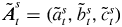 ${{\tilde {\boldsymbol {A}} }}^{s}_t=({{\tilde {a}}}^{s}_t, {{\tilde {b}}}^{s}_t, {{\tilde {c}}}^{s}_t)$ over discrete times
 $s=s_k:=t-k({\rm \Delta} s),$
 $k=0,1,2,\ldots$ by backward integration:
 \begin{equation} {{\tilde{\boldsymbol{A}} }}^{s_k}_t({{ \boldsymbol{x} }}) = {{\tilde{\boldsymbol{A}} }}^{s_{k-1}}_t({{ \boldsymbol{x} }}) - {{\boldsymbol{u}}}({{\tilde{\boldsymbol{A}} }}^{s_{k-1}}_t({{ \boldsymbol{x} }}),s_{k-1}) \, {\rm \Delta} s + \sqrt{2\nu{\rm \Delta} s}\, \tilde{{\boldsymbol{N}}}^{k}, \quad k=1,2,3,\ldots; \quad {{\tilde{\boldsymbol{A}} }}^{t}_t({{ \boldsymbol{x} }})={{ \boldsymbol{x} }}, \end{equation}
see Kloeden & Platen (Reference Kloeden and Platen2013). Here  $\tilde {{\boldsymbol {N}}}^{k}$ is a three-dimensional normal random vector with mean zero and covariance matrix
 ${\boldsymbol {I}},$ independently sampled for each step
 $k=1,2,3,\ldots$ For additive noise, as in the (3.1), the Euler–Maruyama scheme is first-order strongly convergent as
 ${\rm \Delta} s\to 0$. We use the Mersenne Twister algorithm (Matsumoto & Nishimura Reference Matsumoto and Nishimura1998; Matsumoto Reference Matsumoto2011) to produce a pseudo-random sequence of uniform random numbers and we generate samples of normal random numbers pairwise using the transform method of Box & Muller (Reference Box and Muller1958). To numerically approximate the Cauchy invariant as defined in (2.55) or
 \begin{equation} \tilde{{{{\boldsymbol{\omega}}}}}_s({{ \boldsymbol{x} }},t) = ({{\boldsymbol{\nabla}}}_x{{\tilde{\boldsymbol{A}} }}^{s\prime}_t({{ \boldsymbol{x} }}))^{{-}1\,\top}{{{\boldsymbol{\omega}}}}({{\tilde{\boldsymbol{A}} }}^{s\prime}_t({{ \boldsymbol{x} }}),s\vee{{\tilde{\sigma}}}_t({{ \boldsymbol{x} }})) \end{equation}
we must also discretize the evolution equation for the deformation gradient tensors  ${{\tilde {\boldsymbol {D}}}}^{s}_t({{ \boldsymbol {x} }}) :=({{\boldsymbol {\nabla }}}_x{{\tilde {\boldsymbol {A}} }}^{s}_t)^{-1\,\top },$ or the Jacobian derivative matrices of the flow map. The equation for
 ${{\tilde {\boldsymbol {D}}}}^{s}_t({{ \boldsymbol {x} }})$ was already derived in (2.41) and is reproduced here as
 \begin{equation} {\textrm{d}} {{\tilde{\boldsymbol{D}}}}^{s}_t = \left. -{{\tilde{\boldsymbol{D}}}}^{s}_t \boldsymbol{\cdot} ({{\boldsymbol{\nabla}}}_x{{\boldsymbol{u}}})^{\top} \right|_{({{\tilde{\boldsymbol{A}} }}^{s}_t,s)}{\textrm{d}}s , \quad s < t; \quad {{\tilde{\boldsymbol{D}}}}^{t}_t={\boldsymbol{I}} \end{equation}
with the corresponding Euler approximation
 \begin{equation} {{\tilde{\boldsymbol{D}}}}^{s_k}_t = {{\tilde{\boldsymbol{D}}}}^{s_{k-1}}_t \boldsymbol{\cdot} [{\boldsymbol{I}} + ({{\boldsymbol{\nabla}}}_x{{\boldsymbol{u}}})^{\top}|_{({{\tilde{\boldsymbol{A}} }}^{s_{k-1}}_t,s_{k-1})} {\rm \Delta} s], \quad k=1,2,3,\ldots; \quad {{\tilde{\boldsymbol{D}}}}^{t}_t={\boldsymbol{I}}. \end{equation}
To calculate averages a statistically independent ensemble of  $N$ stochastic Lagrangian particles is evolved, with positions
 ${{\tilde {\boldsymbol {A}} }}^{s_k,(n)}_{t}({{ \boldsymbol {x} }})$ and deformation matrices
 ${{\tilde {\boldsymbol {D}}}}^{s_k,(n)}_t({{ \boldsymbol {x} }})$ for
 $n=1,\ldots ,N.$ At every
 $k$th step in time
 $s$, Navier–Stokes solution fields
 ${{\boldsymbol {u}}}$ and
 ${{\boldsymbol {\nabla }}}_x{{\boldsymbol {u}}}$ must be evaluated at the current set of particle locations and used to evolve both them and the deformation matrices backward to the next time. At each time step
 $k$, the algorithm checks whether the
 $n$th particle has left the domain:
 \begin{equation} |{{\tilde{b}}}^{s_k,(n)}_{t}({{ \boldsymbol{x} }})|>h. \end{equation}
If so, this  $n$th particle is declared to have been ‘born’ at that time and evolved no further backward. Interpolation is used to identify the wall hitting time
 $s={{\tilde {\sigma }}}_{*}^{(n)}=s_{k-1}-{\rm \Delta} {{\tilde {\sigma }}}_{*}^{(n)}$ at which the condition
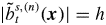 $|{{\tilde {b}}}^{s,(n)}_{t}({{ \boldsymbol {x} }})|=h$ first occurred. Note that
 ${{\tilde {\sigma }}}_{*}^{(n)}$ is a random quantity, even given both
 ${{\tilde {\boldsymbol {A}} }}^{s_{k-1},(n)}_{t}({{ \boldsymbol {x} }})$ and
 ${{\tilde {\boldsymbol {A}} }}^{s_k,(n)}_{t}({{ \boldsymbol {x} }}).$ As discussed in appendix A, this hitting time can be estimated by a stochastic interpolation method that becomes exact in the limit of a vanishing wall-normal velocity, with no restriction whatsoever on the time step
 ${\rm \Delta} s.$ The same interpolation scheme also gives the wall positions
 $(a,c)=(\tilde {a}_*^{(n)}, \tilde {c}_*^{(n)})$ at the first hitting time. Furthermore, the deformation matrix is updated to the hitting time by the Euler formula with a fractional time step
 \begin{equation} {{\tilde{\boldsymbol{D}}}}^{{{\tilde{\sigma}}}_*^{(n)},(n)}_t = {{{\tilde{\boldsymbol{D}}}}^{s_{k-1},(n)}_t} \boldsymbol{\cdot} [{\boldsymbol{I}} + ({{\boldsymbol{\nabla}}}_x{{\boldsymbol{u}}})^{\top}|_{({{\tilde{\boldsymbol{A}} }}^{s_{k-1},(n)}_t,s_{k-1})} {\rm \Delta} {{\tilde{\sigma}}}_*^{(n)}], \end{equation}
and used to evaluate the Cauchy invariant for the newly ‘born’ particle by the formula
 \begin{equation} \tilde{{{{\boldsymbol{\omega}}}}}_*^{(n)} = {{\tilde{\boldsymbol{D}}}}^{{{\tilde{\sigma}}}_*^{(n)},(n)}_t \boldsymbol{\cdot} {{{\boldsymbol{\omega}}}}(\tilde{a}_*^{(n)}, \tilde{b}_*^{(n)}, \tilde{c}_*^{(n)},{{\tilde{\sigma}}}_*^{(n)}), \quad \tilde{b}_*^{(n)}={\pm} h , \end{equation}
requiring the velocity gradient  ${{\boldsymbol {\nabla }}}_x{{\boldsymbol {u}}}$ of the Navier–Stokes solution at space–time point
 $(\tilde {a}_*^{(n)},\tilde {b}_*^{(n)}, \tilde {c}_*^{(n)},{{\tilde {\sigma }}}_*^{(n)}).$ The random values for each newly ‘born’ particle with label
 $n,$
 \begin{equation} {{\tilde{\sigma}}}_*^{(n)}, \ \tilde{a}_*^{(n)},\ \tilde{c}_*^{(n)}, \ \tilde{{{{\boldsymbol{\omega}}}}}_*^{(n)} \end{equation}
are then output to a file. Subsequently, for all of the remaining particles  $n$, the so-called ‘alive’ ones which have not yet hit the wall, the deformation matrix is updated by the Euler formula (3.4) to the new time
 $s_k=s_{k-1}-{\rm \Delta} s$ and then that matrix is used to calculate an updated Cauchy invariant at time
 $s_k$ with
 \begin{equation} \tilde{{{{\boldsymbol{\omega}}}}}_{s_k}^{(n)}({{ \boldsymbol{x} }},t) = {{\tilde{\boldsymbol{D}}}}^{s_{k},(n)}_t\boldsymbol{\cdot} {{{\boldsymbol{\omega}}}}({{\tilde{\boldsymbol{A}} }}^{s_k}_t({{ \boldsymbol{x} }}),s_k), \end{equation}
requiring the Navier–Stokes velocity gradient  ${{\boldsymbol {\nabla }}}_x{{\boldsymbol {u}}}$ at time
 $s_k$ to obtain
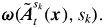 ${{{\boldsymbol {\omega }}}}({{\tilde {\boldsymbol {A}} }}^{s_k}_t({{ \boldsymbol {x} }}),s_k).$
This entire procedure is repeated in all subsequent time steps. The set of stochastic particles labelled by  $n\in {\mathbb {N}}=\{1,2,\ldots ,N\}$ is partitioned into a subset
 ${\mathbb {W}}_k$ representing ‘wall’/‘pre-born’ particles that have already hit the wall by time step
 $k$ and the complementary subset
 ${\mathbb {I}}_k={\mathbb {N}}\backslash {\mathbb {W}}_k$ representing ‘interior’/‘alive’ particles still in the flow interior at time step
 $k.$ At each step, the variables associated to ‘wall’ particles with
 $n\in {\mathbb {W}}_k$ are left unchanged and only the variables associated to ‘interior’ particles with
 $n\in {\mathbb {I}}_k$ are evolved from time
 $s_k$ back to time
 $s_{k+1}.$ Identifying the newly ‘born’ particles, storing the values of their variables at their first hitting time and adding their indices
 $n$ to
 ${\mathbb {W}}_k$ then yields the new sets
 ${\mathbb {W}}_{k+1}\supseteq {\mathbb {W}}_k$ and
 ${\mathbb {I}}_{k+1}={\mathbb {N}}\backslash {\mathbb {W}}_{k+1}$ for the next time step. At every step, ensemble means of random variables
 $\tilde {F}$ are calculated by averaging over the entire set of particles
 ${\mathbb {N}},$ both wall and interior, as
 \begin{equation} {\mathbb{E}}[\tilde{F}] \doteq \frac{1}{N} \sum_{n=1}^{N} \tilde{F}^{(n)} . \end{equation}
The convergence rate of this scheme as  $N\to \infty$ is rather slow, with standard Monte Carlo errors by the central limit theorem of order
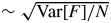 $\sim \sqrt {\textrm {Var}[F]/N}$, where
 $\textrm {Var}[F]$ is the variance of the averaged variable. To obtain numbers of samples
 $N$ sufficiently large, we implemented the preceding algorithm in Fortran on a cluster computer at the Maryland Advanced Research Computing Center. The Monte Carlo averaging scheme is perfectly parallelizable, with statistically independent subsets of samples assigned to distinct cluster nodes and no communication whatsoever required between nodes.
An annotated version of the Fortran code which implements the algorithm discussed above is available at the Github repository (Eyink et al. Reference Eyink, Gupta, Wang and Zaki2019). This code is written to be used with the Johns Hopkins University online channel-flow database, which is discussed next.
3.2. The JHU channel-flow database
The Johns Hopkins turbulence databases (JHTDB) channel-flow dataset (Graham et al. Reference Graham2016) is exploited for the empirical study in this paper. This data was generated from a Navier–Stokes simulation in a channel using a pseudo-spectral method in the plane parallel to the walls and a seventh-order B-splines collocation method in the wall-normal direction (Lee, Malaya & Moser Reference Lee, Malaya and Moser2013). For a numerical solution, the Navier–Stokes equations were formulated in wall-normal velocity–vorticity form (Kim, Moin & Moser Reference Kim, Moin and Moser1987). Pressure was computed by solving the pressure Poisson equation only when writing to disk, which was every five time steps for 4000 snapshots, enough for about one domain flow-through time. The simulation domain  $[0,8{\rm \pi} ] \times [-h,h] \times [0,3{\rm \pi} ]$ with channel half-height
 $h=1$ was discretized using a spatial grid of
 $2048 \times 512 \times 1536$ points in the streamwise (
 $x$), wall-normal (
 $y$) and spanwise (
 $z$) directions, respectively. Time advancement was made with a third-order low-storage Runge–Kutta method and dealiasing was performed with 2/3 truncation (Orszag Reference Orszag1971). A constant pressure head was applied to drive the flow at
 $Re_\tau = 1000$ (
 $Re_{bulk} = {2hU_{bulk}}/{\nu } = 40\,000$) with bulk velocity near unity. As is common, we shall indicate with a superscript ‘
 $+$’ non-dimensionalized quantities in viscous wall units, with velocities scaled by friction velocity
 $u_*$ and lengths by viscous length
 $\delta _\nu =\nu /u_*=10^{-3}.$ Also as usual, we define
 $y^{+}=(h\mp y)/\delta _\nu$ near
 $y=\pm h.$ In these units, the first
 $y$-grid point in the simulation is located at a distance
 ${\rm \Delta} y_1^{+} = 1.65199\times 10^{-2}$ from the wall, while in the centre of the channel
 ${\rm \Delta} y_c^{+} = 6.15507.$ Other numerical parameters of the channel-flow dataset are summarized in table 1.
Simulation parameters for a turbulent channel-flow dataset.

The JHTDB web services supports subroutine-like calls for data that can be made from MATLAB, Fortran and C/C++ programs, including getVelocity for stored velocity data and getVelocityGradient for finite-difference approximations to velocity gradients; see Li et al. (Reference Li, Perlman, Wan, Yang, Meneveau, Burns, Chen, Szalay and Eyink2008), Graham et al. (Reference Graham2016). To return data off the numerical space–time grid, the JHTDB web services provide methods for performing spatial and temporal interpolation within the database. Spatial interpolation is supported using multivariate polynomial interpolation in the barycentric Lagrange form, with stencils containing  $q=4,6,8$ points in each coordinate direction for an order
 $q$ interpolant, so-called Lag4, Lag6, Lag8 methods, respectively. Temporal interpolation is supported using cubic Hermite interpolating polynomials (PCHIPInt), with centred finite-difference evaluation of the endpoint time derivatives, employing a total of four temporal points. Spatial differentiation at grid points is performed using differentiation matrices obtained from the barycentric method of Lagrange polynomial interpolation for
 $q=4,6,8$ points, so-called FD4NoInt, FD6NoInt, FD8NoInt options (Berrut & Trefethen Reference Berrut and Trefethen2004; Graham et al. Reference Graham2016). The FD4Lag4 option provides off-grid space-interpolated gradients with derivatives approximated by the FD4NoInt method at the grid sites and these data are then space interpolated to queried points using the Lag4 method. In the current study, getVelocity is used with Lag6 and PCHIPInt options to obtain off-grid velocity data and getVelocityGradient is used with FD4Lag4 and PCHIPInt options to obtain velocity gradients.
Because the JHTDB turbulent channel-flow dataset was obtained from a numerical simulation with relatively low near-wall resolutions in the streamwise and spanwise directions (see table 1), the vorticity  ${{{\boldsymbol {\omega }}}}({{ \boldsymbol {x} }},t)$ returned by the database in the vicinity of the wall may exhibit observable departures from an exact Navier–Stokes solution. The stochastic Cauchy invariant approximated by (3.7a,b), (3.9) thus cannot be expected to be exactly conserved in time using such numerical data, even if the stochastic Lagrangian integration scheme has
 ${\rm \Delta} s$ sufficiently small and
 $N$ sufficiently large to be very well converged, since discretization errors depending upon
 ${\rm \Delta} x,$
 ${\rm \Delta} y,$
 ${\rm \Delta} z,$
 ${\rm \Delta} t$ will remain. On the other hand, a coarse-grained vorticity field
 \begin{equation} \hat{{{{\boldsymbol{\omega}}}}}({{ \boldsymbol{x} }},t) = \int \textrm{d}^{3}x \, G_{\ell_x}(x-x')G_{\ell_y}(y-y')G_{\ell_z}(z-z')\,{{{\boldsymbol{\omega}}}}({{ \boldsymbol{x} }}',t) \end{equation}
when calculated from the database, with length scales  $\ell _x,$
 $\ell _y,$
 $\ell _z$ each comprising several grid lengths
 ${\rm \Delta} x,$
 ${\rm \Delta} y,$
 ${\rm \Delta} z,$ will plausibly agree with a Navier–Stokes solution coarse grained over the same length scales, with better correspondence than for pointwise fields. Of course, the coarse-grained stochastic Cauchy invariants for a Navier–Stokes solution
 \begin{equation} \hat{\tilde{{{{\boldsymbol{\omega}}}}}}_s({{ \boldsymbol{x} }},t) = \int \textrm{d}^{3}x \,G_{\ell_x}(x-x') G_{\ell_y}(y-y')G_{\ell_z}(z-z')\,\tilde{{{{\boldsymbol{\omega}}}}}_s({{ \boldsymbol{x} }}',t) \end{equation}
will satisfy a corresponding statistical conservation law
 \begin{equation} \hat{{{{\boldsymbol{\omega}}}}}({{ \boldsymbol{x} }},t) = {{\mathbb{E}}}[\hat{\tilde{{{{\boldsymbol{\omega}}}}}}_s({{ \boldsymbol{x} }},t)] \end{equation}
as a direct consequence of the conservation of the fine-grained invariants. If the conjecture is correct that the coarse-grained numerical solutions will agree well with a coarse-grained exact Navier–Stokes solution, then we may expect to observe better conservation numerically for the coarse-grained invariants. To test this hypothesis in our study below, we shall use box/tophat filters with  $\ell _i=n_i ({\rm \Delta} x_i)$ for integers
 $n_i,$
 $i=x,y,z.$ In practice, this means that we locate the grid point
 ${{ \boldsymbol {x} }}_k$ that lies closest to a given point
 ${{ \boldsymbol {x} }}$ and then average over the set of points
 ${{ \boldsymbol {x} }}'$ in the box centred at
 ${{ \boldsymbol {x} }}_k$ and extending
 $n_i/2$ grid spacings to the left and to the right in each coordinate direction
 $i=x,y,z.$ This space average is easily included in our Monte Carlo scheme, by releasing stochastic Lagrangian particles at time
 $t$ with positions
 ${{ \boldsymbol {x} }}'$ chosen at random, uniformly distributed over such a box.
3.3. Validation of the numerical method
We shall now validate the computational algorithms described above by verifying the mean conservation law of the stochastic Cauchy invariant, (2.54). This is a stringent test of our numerical methods to evaluate the Cauchy invariant and its statistics and also of the fidelity of the JHTDB channel-flow dataset to a true Navier–Stokes solution.
3.3.1. Description of the test events and variables
Before presenting numerical results, we must recall that the stochastic Cauchy invariant is a vector quantity, each of whose components  $\tilde {\omega }_{s i}({{ \boldsymbol {x} }},t)$ for
 $i=x,$
 $y,$
 $z$ is conserved on average, with a mean value equal to
 $\omega _i({{ \boldsymbol {x} }},t)$ independent of
 $s<t.$ A coordinate-free decomposition of the stochastic Cauchy invariant can be obtained using the unit vector
 $\hat {{\boldsymbol {n}}}_\omega ({{ \boldsymbol {x} }},t):={{{\boldsymbol {\omega }}}}({{ \boldsymbol {x} }},t)/|{{{\boldsymbol {\omega }}}}({{ \boldsymbol {x} }},t)|$ pointing in the direction of vorticity at final time
 $t,$ which permits definition of parallel and perpendicular components of the Cauchy invariant
 \begin{equation} \tilde{\omega}_{s\|}({{ \boldsymbol{x} }},t):=\tilde{{{{\boldsymbol{\omega}}}}}_{s}({{ \boldsymbol{x} }},t)\boldsymbol{\cdot} \hat{{\boldsymbol{n}}}_\omega({{ \boldsymbol{x} }},t), \quad \tilde{{{{\boldsymbol{\omega}}}}}_{s\perp}({{ \boldsymbol{x} }},t):=\tilde{{{{\boldsymbol{\omega}}}}}_{s}({{ \boldsymbol{x} }},t)-\tilde{\omega}_{s\|}({{ \boldsymbol{x} }},t) \hat{{\boldsymbol{n}}}_\omega({{ \boldsymbol{x} }},t), \end{equation}
which satisfy the mean conservation laws
 \begin{equation} {{\mathbb{E}}}\left[ \tilde{\omega}_{s\|}({{ \boldsymbol{x} }},t)\right] = |{{{\boldsymbol{\omega}}}}({{ \boldsymbol{x} }},t)|, \quad {{\mathbb{E}}}\left[ \tilde{{{{\boldsymbol{\omega}}}}}_{s\perp}({{ \boldsymbol{x} }},t)\right] ={{\textbf{0}}}, \quad s < t. \end{equation}
In our numerical study below we shall present results both for the Cartesian components of the stochastic Cauchy invariant and also for the intrinsic  $\|,$
 $\perp$ components.
We have selected for investigation from the channel-flow database two test vorticity vectors  ${{{\boldsymbol {\omega }}}}({{ \boldsymbol {x} }},t)$, whose detailed space–time coordinates are given in table 2. The choice of these two cases is discussed in detail in Part 2. Here it suffices to note that the spatial coordinates both correspond to points at the bottom of the buffer layer, with
 $y^{+}\simeq 5,$ one at the location of an ‘ejection’ where fluid is erupting away from the wall and the other at a ‘sweep’ where fluid is splatting against the wall. We shall refer to these two events hereafter simply as the ‘ejection’ and the ‘sweep’, respectively.
Coordinates of analysed vorticity vectors.

3.3.2. Statistics of the Cauchy invariant for the ejection event
We first consider the ejection case. In figure 2(a) we plot as functions of  $\delta s=s-t$ the numerically calculated expectation values of the
 $i$th component of the stochastic Cauchy invariant for
 $i=x,$
 $y,$
 $z,$
 $\|,$ and the vector norm
 $|\,{{\mathbb {E}}}[ \tilde {{{{\boldsymbol {\omega }}}}}_{s\perp }({{ \boldsymbol {x} }},t)]|$ for
 $i={\perp}.$ These were obtained with the numerical Monte Carlo scheme in § 3, using integration time step
 ${\rm \Delta} s=10^{-3}$ in (3.1), (3.4) and number of particles
 $N=10^{7}$ to calculate sample averages as in (3.10). According to the mathematical theory for exact Navier–Stokes solutions presented in § 2, the graphs for all components in figure 2(a) should be flat horizontal lines, with values equal to the corresponding components of the vorticity vector
 ${{{\boldsymbol {\omega }}}}({{ \boldsymbol {x} }},t)$ at the final time. While this is reasonably verified at
 $\delta s^{+}>-100$, especially for components
 $i=y,z,\|,$ there are clear deviations at longer times and for other components
 $i=x,\perp .$ It should be emphasized that the ‘naive Cauchy invariants’, which are exactly conserved for smooth Euler solutions, exhibit much larger deviations from conservation for the channel-flow Navier–Stokes solution than do the numerical results in figure 2(a) for the stochastic Cauchy invariants. As discussed in the supplementary material, the ‘naive invariants’ can be accurately evaluated by the same numerical methods as discussed in § 3, by setting the random noise to zero and calculating a standard (deterministic) Lagrangian trajectory and the deformation matrix along it by a fourth-order Runge–Kutta scheme. The results in the supplementary material show that conservation of the ‘naive invariants’ is violated by several orders of magnitude for the same case as in figure 2(a). There is, of course, no reason that conservation of the standard Cauchy invariants should hold for any Navier–Stokes solution and the failure of conservation here confirms previous results that vorticity is not even approximately ‘frozen in’ for a high-Reynolds-number turbulent flow (Guala et al. Reference Guala, Lüthi, Liberzon, Tsinober and Kinzelbach2005, Reference Guala, Liberzon, Lüthi, Kinzelbach and Tsinober2006; Lüthi et al. Reference Lüthi, Tsinober and Kinzelbach2005; Johnson & Meneveau Reference Johnson and Meneveau2016; Johnson et al. Reference Johnson, Hamilton, Burns and Meneveau2017). Nevertheless, despite the much better conservation of the stochastic Cauchy invariants that we observe, the deviations from exact conservation that arise in our various numerical approximations must be clearly understood.
Expectation value ( $a$) and variance (
 $b$) of the components
 $\tilde {\omega }_{s i}^{+}({{ \boldsymbol {x} }},t)$ of the stochastic Cauchy invariant for the selected point
 $({{ \boldsymbol {x} }},t)$ in the ejection event, plotted as functions of
 $\delta s^{+}$, calculated numerically with
 ${\rm \Delta} s=10^{-3}$ and
 $N=10^{7}.$ The thin black lines are linear fits in semilogarithmic coordinates for
 $\delta s^{+}<-75$.

A first possible source of error is the size of the time step. The value of  ${\rm \Delta} s=10^{-3}$ employed for stochastic integration was slightly smaller than the time step
 ${\rm \Delta} t$ employed in the original channel-flow simulation archived in the database (see table 1). Furthermore, as discussed in the supplementary material, we checked that the numerical results with
 ${\rm \Delta} s=10^{-3}$ are essentially unchanged when using a twice smaller value
 ${\rm \Delta} s=5\times 10^{-4}$ over the reduced time range
 $-100<\delta s^{+}<0.$ The average difference over that interval between the values plotted in figure 2(a) and those generated with
 ${\rm \Delta} s=5\times 10^{-4}$ is less than 0.004 for all components. In particular, the average differences for the parallel and perpendicular components over that interval are, respectively, only 0.21 % and 0.79 % of the vorticity magnitude
 $|{{{\boldsymbol {\omega }}}}|.$ Thus, our results appear to be well converged in the time step.
A much larger source of numerical error in the results presented in figure 2(a) is the number of samples  $N$ employed to calculate averages over realizations of the Brownian motion. The error in approximating expectation values from
 $N$-sample averages as in (3.10) is estimated from the central limit theorem on order of magnitude as
 \begin{equation} \delta {{\mathbb{E}}}\left[\tilde{\omega}_{s\,i}({{ \boldsymbol{x} }},t)\right] \sim \sqrt{\frac{\textrm{Var}[\tilde{\omega}_{s\,i}({{ \boldsymbol{x} }},t)]}{N}}. \end{equation}
We can numerically calculate the variances within the same Monte Carlo scheme by using the standard unbiased estimator
 \begin{equation} \textrm{Var}[\tilde{F}] \doteq \frac{1}{N-1} \sum_{n=1}^{N} (\tilde{F}^{(n)}-{\mathbb{E}}[\tilde{F}])^{2}, \end{equation}
and variances of the Cartesian coordinates of the stochastic Cauchy invariant estimated in this manner with  ${\rm \Delta} s=10^{-3},$
 $N=10^{7}$ are plotted in figure 2(b) versus
 $\delta s^{+}.$ After an initial transient period, these variances appear to grow exponentially rapidly backward in time, with
 $\textrm {Var}[\tilde {\omega }_{s\,i}({{ \boldsymbol {x} }},t)]\propto \exp (2\lambda _i(t-s))$ for
 $s\ll t.$ The growth exponents obtained by linear fits of the numerical results over the range
 $\delta s^{+}<-75$ in semilogarithmic coordinates are
 \begin{equation} \lambda_x^{+}=0.0509, \quad \lambda_y^{+}=0.0624, \quad \lambda_z^{+}=0.0596 \end{equation}
in wall units. Recall that, according to (2.50), the stochastic Cauchy invariant evolves in the same manner as does a material line element forward in time, except that the motion is along stochastic Lagrangian trajectories rather than deterministic ones. The exponential growth of variances that we find is thus consistent with the previous study of Johnson et al. (Reference Johnson, Hamilton, Burns and Meneveau2017), who observed Lagrangian chaos in the same channel-flow database that we employ. The instantaneous Lyapunov exponents obtained by Johnson et al. (Reference Johnson, Hamilton, Burns and Meneveau2017) are plotted in their figure 4(b), with values  $2\times 10^{-3}\sim 2\times 10^{-2}$ in the range
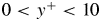 $0<y^{+}<10$, where their non-dimensionalization by a local Kolmogorov time (increasing with
 $y$) corresponds essentially to our wall units. Our growth exponents for the variance are consistent in order of magnitude with those Lyapunov exponents, but are somewhat larger. The somewhat greater values could be due to the fact that we do not average over long times, as Johnson et al. (Reference Johnson, Hamilton, Burns and Meneveau2017) did, and the local stretching rates in our extreme stress event could be larger than average. Also, we do not conditionally sample on a given
 $y^{+}$-value as Johnson et al. (Reference Johnson, Hamilton, Burns and Meneveau2017) did, and the stochastic Lagrangian trajectories released at
 $y^{+}=5.35$ can disperse into the buffer layer where local stretching rates are highest (Johnson et al. Reference Johnson, Hamilton, Burns and Meneveau2017).
The errors in the mean values estimated from the central limit theorem, using (3.16) and the variance calculated by (3.17), explain the largest deviations from exact conservation observed in figure 2(a). For 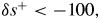 $\delta s^{+}<-100,$ all of the observed deviations are consistent in order of magnitude with fluctuations due to finite
 $N.$ Because of the slow Monte Carlo rate of convergence
 $\propto 1/\sqrt {N}$ in (3.16), it would require
 $N\simeq 10^{14}$ samples to achieve accuracy of even a few per cent for
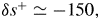 $\delta s^{+}\simeq -150,$ which is beyond our computational means. On the other hand, we estimate from (3.16) that Monte Carlo errors are much less than 1 % for
 $\delta s^{+}>-100.$ This is verified by the observed convergence of the mean values with increasing
 $N$ (not shown) and the smoothness of the plotted curves for
 $\delta s^{+}>-100.$ In that range we see that the components
 $i=y,z,\|$ of the stochastic Cauchy invariant are well conserved in the mean, but there are observable deviations from conservation for
 $i=x,\perp .$ In fact, the mean deviation of the parallel and perpendicular components from conservation over the range
 $-100<\delta s^{+}<0$ are 0.57 % and 2.97 % of the magnitude
 $|{{{\boldsymbol {\omega }}}}|,$ respectively. The final time vorticity direction vector is nearly
 $\hat {{\boldsymbol {n}}}_\omega \simeq \hat {{\boldsymbol {z}}}$ for the case being examined, so that the error in conservation of the perpendicular component arises mainly from non-conservation of the
 $x$-component. These violations of exact conservation are not explained by any numerical artifacts of finite
 ${\rm \Delta} s$ and
 $N$ in our Monte Carlo integration scheme.
The only remaining source of error in our computation is the deviation of the fields stored in the JHTDB channel-flow database from an exact Navier–Stokes solution. Although the numerical simulation stored in the database had excellent spatial resolution in the  $y$-direction near the wall, the wall-parallel resolution was much poorer. As reviewed in table 1,
 ${\rm \Delta} z^{+}=6.1$ and
 ${\rm \Delta} x^{+}=12.3.$ Furthermore, the velocity gradients returned by the database function getVelocityGradient are finite-difference approximations and both velocities and velocity gradients at points off the computational grid are supplied by Lagrangian interpolation. A reasonable estimate of the size of the errors involved in these approximations can be obtained from the deviation of the database velocity gradient matrices from being traceless, as required by flow incompressibility. As we discuss in the supplementary material, we have found that the divergence-free condition is satisfied to a few per cent, with violation less than 0.5 % for
 $y^{+}<10$ but rising up to 3–4 % for
 $y^{+}>30.$ This inaccuracy in the returned velocity gradients accords well with the magnitude of the deviations that we observe in mean conservation of the stochastic Cauchy invariant. An ensemble of stochastic Lagrangian particles released at
 $y^{+}=5.35$ will sample not a resolved Navier–Stokes solution but instead a Lagrange interpolating polynomial, until the ensemble has dispersed over at least several grid lengths in the wall-parallel directions. This is the presumed source of the slight non-conservation observed for
 $i=x,\perp$ components at times
 $\delta s^{+}>-100$ in figure 2(a). To test this explanation, we have numerically generated the coarse-grained stochastic Cauchy invariant defined in (3.12) for filter lengths
 $\ell _i= n_i ({\rm \Delta} x_i)$ in the coordinate directions,
 $i=x$,
 $y$,
 $z,$ using the Monte Carlo scheme discussed in § 3.1. As discussed in Part 2,
 $(n_x,n_y,n_z)=(4,0,4)$ is a reasonable choice of filtering lengths which does not obscure the essential physics of the ejection event under consideration.
Plotted in figure 3 are the mean and variance of the coarse-grained stochastic Cauchy invariant for the selected point, filtered over  $(n_x,n_y,n_z)=(4,0,4)$ grid points. The fluctuations of the mean values for
 $\delta s^{+}<-100$ are increased compared with the unfiltered case shown in figure 2(a), because the empirical average over
 $N$ samples is now doing double duty to represent both the expectation over the Brownian motion and the space average over the filtering box. As can be seen from figure 3(b), the variances of the coarse-grained Cauchy invariant are somewhat increased relative to those plotted in figure 2(b), because the former includes both stochastic and spatial fluctuations. On the other hand, as expected, the mean conservation of the coarse-grained Cauchy invariant is observed in figure 3(a) to be improved for
 $\delta s^{+}>-100$ when compared with the fine-grained means plotted in figure 2(a), especially for the
 $i=x,$
 $\perp$ components. The average deviation from conservation of the parallel and perpendicular components is now found to be 0.79 % and 1.22 % of the magnitude
 $|\hat {{{{\boldsymbol {\omega }}}}}|,$ respectively. We have found that increasing
 $n_x,$
 $n_z$ further (not shown) improves the mean conservation, while the spatial structures become more diffuse. Since mean conservation of the stochastic Cauchy invariant is a quite stringent test of validity of a Navier–Stokes solution, these results validate both our Monte Carlo numerical method to calculate the stochastic Cauchy invariant and also the adequacy of the JHTDB channel-flow database to investigate the turbulent buffer layer.
Expectation value ( $a$) and variance (
 $b$) of the components
 $\hat {\tilde {\omega }}_{s i}^{+}({{ \boldsymbol {x} }},t)$ of the coarse-grained Cauchy invariant for the selected point
 $({{ \boldsymbol {x} }},t)$ in the ejection event, plotted as functions of
 $\delta s^{+}$, calculated numerically with
 ${\rm \Delta} s=10^{-3}$ and
 $N=10^{7}.$ The thin black lines are linear fits in semilogarithmic coordinates for
 $\delta s^{+}<-75$.

3.3.3. Statistics of the Cauchy invariant for the sweep event
We now consider, more briefly, the sweep event. We again investigate the mean conservation of the stochastic Cauchy invariant as a check on our numerical approximations. Figure 4 plots the results for the mean and the variance of the components of the Cauchy invariant, calculated by our Monte Carlo integration scheme with time step  ${\rm \Delta} s=10^{-3}$ and with number of samples
 $N=10^{7}.$ As for the ejection event, we have performed a convergence analysis in
 ${\rm \Delta} s$ (see supplementary material) and found that the results do not change significantly with a smaller time step
 ${\rm \Delta} s=5\times 10^{-4}.$ Over the reduced interval
 $-100<\delta s^{+}<0$ the mean differences in results for the two time steps differ by less than 0.005 for all components, and the mean differences for the parallel and perpendicular components are only 0.38 % and 0.45 % of the magnitude
 $|{{{\boldsymbol {\omega }}}}|,$ respectively. Due to the finite values of
 $N,$ however, the results for
 $\delta s^{+}<-100$ exhibit very large errors, consistent with the variances plotted in figure 4(b). The results for
 $-100<\delta s^{+}<0$ on the other hand are well converged in
 $N,$ so that any residual errors in those results are due to a lack of resolution in the archived channel-flow simulation. Mean conservation holds quite well for the
 $y$,
 $z$ components of the stochastic Cauchy invariant in the time interval
 $-100<\delta s^{+}<0$ for this sweep event, but the
 $x$-component is less well conserved. Quantitatively, the mean deviations from conservation of the parallel and perpendicular components are 2.29 % and 5.01 % of the vorticity magnitude
 $|{{{\boldsymbol {\omega }}}}|,$ respectively. We have again found that spatial coarse graining noticeably improves mean conservation, although a bit less well than it did in the ejection case. The mean deviations from conservation of the parallel and perpendicular components are now 1.43 % and 3.32 % of the vorticity magnitude
 $|\hat {{{{\boldsymbol {\omega }}}}}|,$ respectively. We present plots of the coarse-grained stochastic Cauchy invariant for the sweep case in figure 5, where improved conservation can be observed especially for
 $-50<\delta s^{+}<0.$
Expectation value ( $a$) and variance (
 $b$) of the components
 $\tilde {\omega }_{s i}^{+}({{ \boldsymbol {x} }},t)$ of the stochastic Cauchy invariant for the selected point
 $({{ \boldsymbol {x} }},t)$ in the sweep event, plotted as functions of
 $\delta s^{+}$, calculated numerically with
 ${\rm \Delta} s=10^{-3}$ and
 $N=10^{7}.$ The thin black lines are linear fits in semilogarithmic coordinates for
 $\delta s^{+}<-75$.

Expectation value ( $a$) and variance (
 $b$) of the components
 $\hat {\tilde {\omega }}_{s i}^{+}({{ \boldsymbol {x} }},t)$ of the coarse-grained Cauchy invariant for the selected point
 $({{ \boldsymbol {x} }},t)$ in the sweep event, plotted as functions of
 $\delta s^{+}$, calculated numerically with
 ${\rm \Delta} s=10^{-3}$ and
 $N=10^{7}.$ The thin black lines are linear fits in semilogarithmic coordinates for
 $\delta s^{+}<-75$.

The growth exponents for the variances in the sweep case obtained by linear fits over the range  $\delta s^{+}<-75$ in semilogarithmic coordinates are
 \begin{equation} \lambda_x^{+}=0.1039, \quad \lambda_y^{+}=0.1055, \quad \lambda_z^{+}=0.1069. \end{equation}
These are about double the exponents reported in (3.18a--c) for the ejection event. The greater size is reasonable, since in the sweep event the stochastic particles moving backward in time are lifted up by the flow higher into the buffer layer where local stretching rates are largest (Johnson et al. Reference Johnson, Hamilton, Burns and Meneveau2017). Just as for the ejection considered previously, we conclude that the stochastic Cauchy vector at time  $s$ is exponentially stretched and rotated by transport from
 $s$ to
 $t,$ as pictured in the middle panel of figure 1. An important implication is that the constant mean of the stochastic Cauchy invariant demonstrated in figures 2(a) and 4(a) is due to extensive cancellations of much larger magnitude vorticity vectors for individual realizations. We shall explore this finding further in Part 2.
4. Conclusions and prospects
We have explained the Constantin & Iyer (Reference Constantin and Iyer2008, Reference Constantin and Iyer2011) theory for Navier–Stokes solutions as a stochastic Lagrangian representation in the Kuz'min (Reference Kuz'min1983)–Oseledets (Reference Oseledets1989) formulation of the equation. The theory yields exact mean conservation laws for stochastic Cauchy invariants (in the generalized sense of Besse & Frisch Reference Besse and Frisch2017) corresponding both to vortex momentum and to vorticity. For wall-bounded flows, these conservation laws yield an exact representation of vorticity at any interior point as an average over stochastic vorticity contributions transported from the wall. We discussed some relations of the Constantin & Iyer (Reference Constantin and Iyer2008, Reference Constantin and Iyer2011) results with the Eulerian theory of Lighthill (Reference Lighthill and Rosenhead1963)–Morton (Reference Morton1984) for the generation of vorticity at solid walls. We have also elaborated a numerical Monte Carlo method to calculate the stochastic Cauchy invariants and their statistics, given the Eulerian flow fields in space–time. These results hold for every Navier–Stokes solution, laminar as well as turbulent. We believe that the theory justifies stochastic Lagrangian flows as natural for viscous hydrodynamics, providing deeper analysis and insights into nonlinear vortex dynamics than the deterministic Lagrangian trajectories more suited to ideal fluids. In particular, the stochastic formulation fully represents the creation of vorticity at solid walls and its diffusion into the interior.
In Part 2, we shall apply these exact mathematical and computational tools to investigate a concrete problem, the process of ‘lifting’ of vortex lines from the wall into the buffer layer of a turbulent channel flow. The present paper has validated the numerical Lagrangian scheme proposed in this work when used in conjunction with the simulation database for channel-flow turbulence documented by Graham et al. (Reference Graham2016). In particular, we have shown that the stochastic Cauchy invariant calculated by our methods has a well-conserved mean value, providing a stringent test on the fidelity of the numerical results to an exact Navier–Stokes solution. In the following paper, we shall explore the implications of the large cancellations in the conserved means of the stochastic Cauchy invariants which is implied by the exponential growth in their variances. We shall compare there our results and conclusions with those drawn from earlier experimental and computational studies. The long term goal of this line of research is to understand in detail the Lagrangian evolution of vorticity generated at the wall and to explicate the mechanisms by which a constant mean flux of spanwise vorticity is maintained.
An important related direction for future work is more efficient numerical methods. In this paper we have developed and applied the simplest Monte Carlo scheme with an Euler–Maruyama discretization of the equations of motion for stochastic Lagrangian particles. Unfortunately, the convergence rate in a number of samples is quite slow, which significantly limits the range of applications. Within standard Monte Carlo, importance sampling techniques, e.g. by change of drift (Arouna Reference Arouna2004), can provide variance reduction and more efficient sampling of rare events. To get a fundamental improvement of Monte Carlo rates of convergence, however, alternatives such as quasi-Monte Carlo (Hofmann & Mathé Reference Hofmann and Mathé1997) and multilevel Monte Carlo (Higham et al. Reference Higham, Mao, Roj, Song and Yin2013) should be explored. We believe that development of such improved numerical schemes is well worth the effort, since stochastic Lagrangian analysis provides unique information on the flow physics not accessible by other means.
There are also clear directions for further work on mathematical and physical theory. As we shall discuss in upcoming work, the stochastic Lagrangian approach of Constantin & Iyer (Reference Constantin and Iyer2008, Reference Constantin and Iyer2011) may be directly related to the Eulerian theory of Lighthill (Reference Lighthill and Rosenhead1963)–Morton (Reference Morton1984) for vorticity generation at the wall. Closer ties should also exist with the Taylor (Reference Taylor1932)–Huggins (Reference Huggins1994) relation, which continues the mean vorticity flux into the interior of the flow. Our discussion in § 2.3 relates the stochastic Lagrangian trajectories to the Eulerian vorticity flux  ${{\boldsymbol {\Sigma }}}$ integrated over any closed, bounded surface, but this result holds with any possible choice of flux. For example,
 $\Sigma _{ij}^{*}:=\epsilon _{ijk} \dot {u}_k$ is a perfectly acceptable definition of a ‘vorticity flux’ which satisfies the balance equation (1.3), but its long-time average in the steady state is zero! It should be possible to measure the distinguished flux (1.2a,b) directly with stochastic trajectories, either pointwise or integrated over wall-parallel planes. If so, interesting physics questions could be addressed, such as how the fresh vorticity injected at the wall is transported subsequently throughout the flow. Without a detailed proof, we note that an apparently natural measure of vorticity flux in terms of the stochastic Cauchy invariant can be calculated as
 \begin{equation} \lim_{s\to t-} \frac{1}{t-s}{{\mathbb{E}}}[({{ \boldsymbol{x} }}-{{\tilde{\boldsymbol{A}} }}^{s}_t({{ \boldsymbol{x} }}))\times \tilde{{{{\boldsymbol{\omega}}}}}_s({{ \boldsymbol{x} }},t)]= {{\boldsymbol{u}}}({{ \boldsymbol{x} }},t)\times {{{\boldsymbol{\omega}}}}({{ \boldsymbol{x} }},t)-2\nu{{\boldsymbol{\nabla}}}\times {{{\boldsymbol{\omega}}}}({{ \boldsymbol{x} }},t). \end{equation}
The viscous contribution in (4.1) differs from that in the Eulerian flux (1.2a,b) by a factor of two, unfortunately, although this calculation does suffice to show that there must be organized vorticity transport by stochastic trajectories in the steady state. Another theoretical topic deserving further work is the discrete approximation of continuous flows suggested by both Kuz'min (Reference Kuz'min1983) and Oseledets (Reference Oseledets1989) in terms of  $N$ point dipoles satisfying the Roberts (Reference Roberts1972) equations. Fluid turbulence makes it natural to consider the statistical mechanics of such dipole systems. Just as with point vortices, the regime of interest to statistical hydrodynamics is a non-extensive, high-energy limit with the flow volume fixed and the energy growing
 $\propto N^{2}$ (Eyink & Spohn Reference Eyink and Spohn1993). Finally, stochastic action principles analogous to that of Eyink (Reference Eyink2010) can be investigated within the Kuz'min (Reference Kuz'min1983)–Oseledets (Reference Oseledets1989) framework, especially for wall-bounded flows. It would be interesting to know in that case whether the conservation laws (2.52), (2.54) for stochastic Cauchy invariants can be derived as consequences of particle-relabelling symmetry.
Acknowledgements
We are grateful to B. Dubrulle and C. Meneveau for useful discussions and suggestions on this paper. We acknowledge the NSF grant BigData:OCE-1633124 for support and G.E. also acknowledges the Simons Foundation through Targeted Grant in MPS-663054 for partial support. This research project was conducted using simulation data from the Johns Hopkins turbulence database (JHTDB) and scientific computing services at the Maryland Advanced Research Computing Center (MARCC).
Declaration of interests
The authors report no conflict of interest.
Supplementary material
Supplementary material is available at https://doi.org/10.1017/jfm.2020.491.
Appendix A. Stochastic interpolation for hitting times and locations
We consider first the stochastic interpolation for the hitting time  $\tilde {s}_*$ based upon the wall-normal coordinate
 $\tilde {b}(s)$ of the stochastic particle. We suppose that the numerical integration has given
 $\tilde {b}(s_i)=b_i$,
 $i=0,1$ for times
 $s_1<s_0$ with
 $|b_0|<h$ and
 $|b_1|>h.$ For a particle hitting the wall at
 $b=\pm h,$ the change of coordinates
 $b\to b'=h \mp b$ transforms the crossing into the event
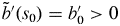 $\tilde {b}'(s_0)=b_0'>0$ and
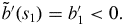 $\tilde {b}'(s_1)=b_1'<0.$ Hereafter we assume this transformation has been made and drop the primes. For small
 ${\rm \Delta} s=s_0-s_1,$ the particle process can be written at times
 $s\in (s_1,s_0)$ as
 \begin{equation} \tilde{b}(s) = b_0 + v(s-s_0) -\sqrt{2\nu}\, \tilde{W}_2(s), \end{equation}
where  $\tilde {W}_2(s)$ for
 $s<s_0$ is a time-reversed Brownian motion with
 $\tilde {W}_2(s_0)=0.$ Imposing the conditions
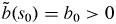 $\tilde {b}(s_0)=b_0>0$ and
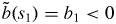 $\tilde {b}(s_1)=b_1<0$ then implies that
 $\tilde {W}_2(s)$ is a generalized Brownian bridge satisfying, for
 ${\rm \Delta} b:=b_0-b_1>b_0>0$,
 \begin{equation} \tilde{W}_2(s_0)=0<\frac{b_0}{\sqrt{2\nu}} , \quad \tilde{W}_2(s_1)=\frac{{\rm \Delta} b - v{\rm \Delta} s}{\sqrt{2\nu}} > \frac{b_0 - v{\rm \Delta} s}{\sqrt{2\nu}}. \end{equation}
The first hitting time  $\tilde {s}_*\in (s_1,s_0)$ when
 $\tilde {b}(\tilde {s}_*)=0$ then corresponds to the largest crossing time of the straight line
 $b=(b_0+v(s-s_0))/\sqrt {2\nu }$ and the Brownian bridge
 $\tilde {W}_2(s)$, or
 \begin{equation} \tilde{W}_2(s) = \frac{b_0+v(s-s_0)}{\sqrt{2\nu}} .\end{equation}
Determining this hitting time  $\tilde {s}_*$ can be mapped, by a sequence of transformations, onto a solved problem of determining the first hitting time of a standard Brownian motion with a straight line. First,
 $\tilde {W}_2(s)$ can be related to a standard Brownian bridge
 $\tilde {B}^{(0)}_2(s),$ satisfying
 \begin{equation} \tilde{B}^{(0)}_2(s_0) =0, \quad \tilde{B}^{(0)}_2(s_1)=0, \end{equation}
by the transformation
 \begin{equation} \tilde{W}_2(s) = \left[\frac{{\rm \Delta} y - v{\rm \Delta} s}{\sqrt{2\nu}}\right] \frac{s-s_0}{s_1-s_0} + \tilde{B}^{(0)}_2(s); \end{equation}
see Borodin & Salminen (Reference Borodin and Salminen2015, Part I, Chapter IV.4.21, p. 64, final statement). The first hitting time  $\tilde {s}_*$ is then determined as the largest time
 $s$ such that
 \begin{equation} \tilde{B}^{(0)}_2(s) = \frac{1}{\sqrt{2\nu}} \frac{b_0(s_1-s)+b_1(s-s_0)}{s_1-s_0}. \end{equation}
Next, the standard Brownian bridge  $\tilde {B}^{(0)}_2(s)$ can be mapped onto a standard Brownian motion
 $\tilde {B}_2(\sigma )$ via the transformation
 \begin{equation} \tilde{B}^{(0)}_2(s) = \frac{s_1-s}{\sqrt{{\rm \Delta} s}} \tilde{B}_2\left(\frac{s-s_0}{s_1-s}\right) , \end{equation}
with the non-negative, dimensionless time variable  $\sigma :=({s-s_0})/({s_1-s})\in [0,\infty )$; see Borodin & Salminen (Reference Borodin and Salminen2015, Part I, Chapter IV.4.21(b), p. 64). The first hitting time is then given by the inverse formula
 $\tilde {s}_*=({s_0+\tilde {\sigma }_*s_1})/({1+\tilde {\sigma }_*})$, where
 $\tilde {\sigma }_*$ is the smallest time
 $\sigma$ such that
 \begin{equation} \tilde{B}_2(\sigma) = \frac{b_0+b_1\sigma}{\sqrt{2\nu{\rm \Delta} s}} =\alpha-\beta\sigma, \qquad \alpha = \frac{b_0}{\sqrt{2\nu{\rm \Delta} s}}, \quad \beta=\frac{|b_1|}{\sqrt{2\nu{\rm \Delta} s}} . \end{equation}
Equivalently,  $\tilde {s}_*=s_0-{\rm \Delta} \tilde {s}_*$ with
 ${\rm \Delta} \tilde {s}_*={\rm \Delta} s ({\tilde {\sigma }_*}/({1+\tilde {\sigma }_*}))$.
The statistical distribution of the first hitting time  $\tilde {\sigma }_*$ of a standard Brownian motion
 $\tilde {B}_2(\sigma )$ and the straight line
 $\alpha -\beta \sigma$ is well known to have the form
 \begin{equation} p(\sigma) = \frac{|\alpha|}{\sqrt{2{\rm \pi} \sigma^{3}}}\exp\left( - \frac{(\alpha-\beta\sigma)^{2}}{2\sigma}\right) = \left(\frac{\lambda}{2{\rm \pi} \sigma^{3}}\right)^{1/2} \exp\left( - \frac{\lambda(\sigma-\mu)^{2}}{2\mu^{2}\sigma}\right) \end{equation}
with parameters
 \begin{equation} \lambda=\alpha^{2} = \frac{b_0^{2}}{2\nu{\rm \Delta} s}, \quad \mu = \frac{\alpha}{\beta} = \left|\frac{b_0}{b_1}\right|; \end{equation}
see Borodin & Salminen (Reference Borodin and Salminen2015, Part II, formula 2.02, p. 295). In the second form, this probability density is known as the inverse Gaussian distribution  $\textrm {IG}(\mu ,\lambda )$ with parameters
 $\mu ,$
 $\lambda$ (Chhikara & Folks Reference Chhikara and Folks1988). A simple algorithm was devised by Michael, Schucany & Haas (Reference Michael, Schucany and Haas1976) to obtain realizations
 $\tilde {\sigma }_*$ drawn from the distribution
 $\textrm {IG}(\mu ,\lambda )$ by a transformation of a normal random variable
 $\tilde {N}$. One first constructs a chi-square random variable
 \begin{equation} \tilde{\chi} = \mu \tilde{N}^{2} \end{equation}
and then sets
 \begin{equation} \tilde{\xi} = 1 + (\tilde{\chi} -\sqrt{4\lambda\tilde{\chi}+\tilde{\chi}^{2}})/2\lambda.\end{equation}
Finally, with probability  $1/(1+\tilde {\xi })$ one selects
 $\tilde {\sigma }_*=\mu \tilde {\xi }$ and otherwise selects
 $\tilde {\sigma }_*=\mu /\tilde {\xi }.$ Below is a snippet of a Fortran code which implements this algorithm:
 \[ \begin{array}{l} \mbox{n1=normal} \cr \mbox{chi=mu*n1**2} \cr \mbox{xi=chi-sqrt(abs(4*lambda*chi+chi**2))} \cr \mbox{xi=1+xi/(2*lambda)} \cr \mbox{u1=uniform} \cr \mbox{if (u1 .le. 1/(1+xi)) then} \cr \quad \mbox{sigma=mu*xi} \cr \mbox{else} \cr \quad \mbox{sigma=mu/xi} \cr \mbox{end if} \end{array} \]
For constant wall-normal velocity  $v$, the above algorithm is exact with no constraint on the size of
 ${\rm \Delta} s$ and it gives a statistically correct sampling of
 $\tilde {\sigma }_*$ and
 $\tilde {s}_*=({s_0+\tilde {\sigma }_*s_1})/({1+\tilde {\sigma }_*})$. In an incompressible fluid flow the wall-normal velocity decreases to zero quadratically with the distance to the wall, so the algorithm should again provide an excellent approximation.
Streamwise and spanwise locations of the stochastic Lagrangian particle at the first hitting time  $\tilde {s}_*$ can be obtained in a statistically accurate fashion by a similar approach. For example, suppose that the streamwise position at the two integration times takes on the values
 $\tilde {a}(s_0)=a_0$,
 $\tilde {a}(s_1)=a_1.$ Between them it is accurately represented for small
 ${\rm \Delta} s$ by the equation
 \begin{equation} \tilde{a}(s) = a_0 + u(s-s_0) + \sqrt{2\nu}\, \tilde{W}_1(s), \end{equation}
with  $\tilde {W}_1(s)$ for
 $s<s_0$ another time-reversed Brownian motion satisfying
 $\tilde {W}_1(s_0)=0.$ Imposing the second endpoint condition on
 $\tilde {a}(s_1)$ then implies that
 $\tilde {W}_1(s)$ becomes a generalized Brownian bridge satisfying
 \begin{equation} \tilde{W}_1(s_0)=0, \quad \tilde{W}_1(s_1)= \frac{{\rm \Delta} a - u{\rm \Delta} s}{\sqrt{2\nu}}. \end{equation}
We now make the same transformations as before, namely
 \begin{equation} \tilde{W}_1(s)= \left(\frac{{\rm \Delta} a - u{\rm \Delta} s}{\sqrt{2\nu}}\right) \frac{s-s_0}{s_1-s_0} + \tilde{B}^{(0)}_1(s) \end{equation}
for a standard Brownian bridge  $\tilde {B}^{(0)}_1(s)$ and
 \begin{equation} \tilde{B}^{(0)}_1(s) = \frac{s_1-s}{\sqrt{{\rm \Delta} s}} \tilde{B}_1(\sigma) = \frac{\sqrt{{\rm \Delta} s}}{1+\sigma} \tilde{B}_1(\sigma) \end{equation}
for a standard Brownian motion  $\tilde {B}_1(\sigma )$ with
 $\sigma =({s-s_0})/({s_1-s})$. Together these give
 \begin{equation} \tilde{a}(s) = \frac{a_0 (s_1-s)+ a_1 (s-s_0)}{s_1-s_0} + \frac{\sqrt{2\nu{\rm \Delta} s}}{1+\sigma} \tilde{B}_1(\sigma), \end{equation}
which is linear interpolation with a stochastic correction. In particular, the streamwise location at the time  $\tilde {s}_*$ of first hitting of the wall is
 \begin{equation} \tilde{a}_*:=\tilde{a}(\tilde{s}_*) = \frac{a_0 (s_1-\tilde{s}_*)+ a_1 (\tilde{s}_*-s_0)}{s_1-s_0} + \frac{\sqrt{2\nu{\rm \Delta} s}}{1+\tilde{\sigma}_*} \tilde{B}_1(\tilde{\sigma}_*). \end{equation}
Likewise, the spanwise location is
 \begin{equation} \tilde{c}_*:=\tilde{c}(\tilde{s}_*) = \frac{c_0 (s_1-\tilde{s}_*)+ c_1 (\tilde{s}_*-s_0)}{s_1-s_0} + \frac{\sqrt{2\nu{\rm \Delta} s}}{1+\tilde{\sigma}_*} \tilde{B}_3(\tilde{\sigma}_*). \end{equation}
The two new Brownian motions at the single time  $\tilde {\sigma }_*$ are statistically represented by
 $\tilde {B}_i(\tilde {\sigma }_*)=\sqrt {\tilde {\sigma }_*}\tilde {N}_i,$
 $i=1,3$ where
 $\tilde {N}_1,$
 $\tilde {N}_3$ are new independent normal random variables.