THE EVIDENCE FOR PROCYCLICAL TFP

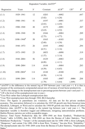
The evidence for the persistence of procyclical TFP and the stability of the cyclicality coefficient comes from a series of regressions of the change in the natural log of TFP (δlnTFP) on the change in the unemployment rate in percentage points (δUR):

The estimated constant term in the equation (?) can be interpreted as an estimate of the trend growth rate of TFP over the period studied. The coefficient (?) describes the relationship between the TFP growth rate and the change in the unemployment rate, and is thus a measure of cyclicality.

The statistical analysis covers more than a century of data for the U.S. private nonfarm economy, which has typically accounted for about three-fourths of GDP. The declining share of agriculture and the rising share of government have kept the private nonfarm economy's share roughly stable. Prior empirical work on productivity has typically involved shorter data runs and has often focused on the manufacturing sector alone. Although data for manufacturing are more detailed than those available for the rest of the economy, trends within the sector do not necessarily offer an accurate guide to what is happening in the economy as a whole. Manufacturing has contributed a declining share of U.S. GDP, particularly since the 1970s. Even at its high point in the mid-century decades, that share barely exceeded one-third, and today it contributes less than one-sixth.Footnote ³

The regressions reported in Table 1 have at least two notable features. First, the coefficients on the change in the unemployment rate all lie within a tight range bounded by –.83 for the post-World War II era (regression 1.8) and –1.03 for the entire period from 1890 to 2004 and (regression 1.10).Footnote ⁴ Over more than a century, TFP was procyclical in a remarkably consistent fashion: a fall in the unemployment rate by one percentage point led to an increase in the growth rate of TFP of about 0.9 percent per year. The procyclical relationship held across all time periods, even the World War II years, despite the fact that nearly half of all production went to the military and there were shortages and rationing in the civilian sector.Footnote ⁵ Nor does the size of the procyclicality coefficient depend on whether one is close to potential output or substantially below it. A comparison of regressions 1.10 and 1.11 shows that inclusion of the level of unemployment (UR) along with its change (ΔUR) has little effect on the originally estimated coefficient.

TABLE 1

THE PROCYCLICAL BEHAVIOR OF TFP, 1890–2004

^aΔlnTFP is the difference in the natural log of TFP between year t and year t-1. It is thus a measure of the continuously compounded annual rate of increase of total factor productivity.

^bΔUR is the change in the unemployment rate in percentage points between year t and year t-1.

^cUR is the level of the unemployment rate in year t.

^d Uses Weir rather than Lebergott unemployment data

^e Uses Weir unemployment data through 1948, BLS thereafter.

Notes:

The figures in parentheses are t-statistics. All data are for the private nonfarm economy. The convention followed is to calculate the 1947/48 growth rate from historical data (Kendrick, Lebergott, or Weir) and to calculate the 1948/49 growth rate from Bureau of Labor Statistics data. ΔlnTFP is the change in the natural log between year t and year t–1. The dependent variable is therefore logged and differenced, mitigating autocorrelation problems. Durbin-Watson statistics are within acceptable ranges.

Sources:

Total Factor Productivity data for 1890–1948 are from Kendrick, “Productivity Trends,” table A-XXIII); data for 1948–2004 are from the Bureau of Labor Statistics, “Net Multifactor Productivity.” Variant 1 of the unemployment rate for 1890–1948 is from Lebergott, “Manpower,” and variant 2 for 1890–1948 is from Weir, “Century.” See also Weir, “Reliability.” The unemployment rates for 1948–2004 come from the Bureau of Labor Statistics, “Employment Status.”

It is striking that the estimates pre- and post-World War II are so similar. Although John Kendrick felt comfortable publishing annual TFP estimates, Simon Kuznets worried about the use of his early national income estimates for cyclical analysis, primarily because of unease about the inventory investment series he had constructed.Footnote ⁶ There are many ways in which inaccurate data might lead to spurious conclusions. But if the process producing short-run procyclicality was similar prewar and postwar, and if there was simply more noise in the prewar data, we might have expected the estimated prewar relationship to be weaker. It is not.

Table 1 also illustrates how much TFP growth rates varied in different historical epochs, a finding emphasized in the work of Moses Abramovitz and other pioneers in the study of TFP growth rates.Footnote ⁷ The trend growth rates represented by the estimates of the constant term vary from a low of 0.53 percent per year during the “dark ages” from 1973 to 1995 (regression 1.7) to 1.95 during the golden age from 1948 to 1973 (regression 1.6) to a high of 2.83 percent per year in the Depression years from 1929 to 1941 (regression 1.1).

This variation in trend growth rates measured between business cycle peaks is consistent with a view that the arrival of economically important innovations may be quite discontinuous, and cluster in particular epochs, rendering some periods more technologically progressive than others. A contrasting perspective underlies the mechanical use of the Hodrick-Prescott filter to separate trend from cycle in real business cycle studies. These studies are not concerned with identifying business cycle peaks, nor do they use such identifications to calculate varying trend growth rates. They envision a relatively smooth long run process of technological change, perturbed by deviations upwards and downwards from trend in the growth rate of TFP. These deviations are considered to be exogenous, rather than the consequence of demand shocks that might widen or shrink an output gap, and are assumed to be the impulses generating cyclical movements in GDP.Footnote ⁸

PROCYCLICALITY IN TFP AND OUTPUT PER HOUR

Interest in the procyclicality of TFP is relatively recent.Footnote ⁹ Since the 1960s and the work of Thor Hultgren, Thomas Wilson and Otto Eckstein, and Edwin Kuh, however, empirical macroeconomists have taken it as a stylized fact that the growth of labor productivity is procyclical, which means that the growth rate of output per hour (like TFP) is negatively related to changes in the unemployment rate.Footnote ¹⁰ The majority of these studies deal with data from manufacturing, but Robert Gordon makes the claim more generally for the private nonfarm economy.Footnote ¹¹

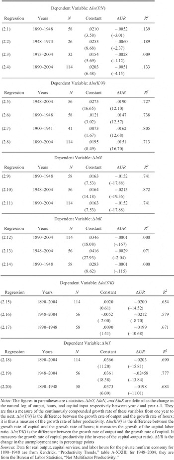
Table 2 explores the cyclicality of output per hour and related measures as well as their long-run growth paths. Its regressions replace the TFP growth rate in Table 1 with other dependent variables, including the growth rates of output per hour, the capital-labor ratio, hours, capital, output per unit of capital, and total output. The results show first (regressions 2.1–2.4) that although output per hour, like TFP, is procyclical, the relationship between its growth rate and the change in the unemployment rate is weaker, and for the period after 1973 (regression 2.3), one cannot reject the hypothesis of acyclicality. In an arithmetical sense, the procyclicality of labor productivity is due to the fact that the response of output to a change in the unemployment rate (regressions 2.18–20) is stronger than the response of hours (regressions 2.9–11).

TABLE 2

THE CYCLICAL BEHAVIOR OF LABOR PRODUCTIVITY, CAPITAL PRODUCTIVITY, THE CAPITAL–OUTPUT RATIO, AND THEIR COMPONENTS

Notes:

The figures in parentheses are t-statistics. ΔlnY, ΔlnN, and ΔlnK are defined as the change in the natural log of output, hours, and capital input respectively between year t and year t–1. They are thus a measure of the continuously compounded growth rate of these variables from one year to the next. Δln(Y/N) is the difference between the growth rate of output and the growth rate of hours; it is thus a measure of the growth rate of labor productivity. Δln(K/N) is the difference between the growth rate of capital and the growth rate of hours; it measures the growth of the capital-labor ratio. Δln(Y/K) is the difference between the growth rate of output and the growth rate of capital. It measures the growth rate of capital productivity (the inverse of the capital-output ratio). ?UR is the change in the unemployment rate in percentage points

Sources:

Data for real output, capital services, and labor hours for the private nonfarm economy for 1890–1948 are from Kendrick, “Productivity Trends,” table A-XXIII; for 1948–2004, they are from the Bureau of Labor Statistics, “Net Multifactor Productivity.”

Whereas both output and hours change systematically with a change in the unemployment rate, the coefficient in the capital growth rate equation is so small that the growth rate in capital appears to be acyclical (regressions 2.12–14). Why? There are substantial lead times in acquiring some types of producer durables (aircraft, for example) as well as virtually all categories of structures (factories, warehouses, houses, and any type of infrastructure). These long gestation periods, in which projects are completed in an uncertain future and where the strength of aggregate demand down the road can only be guessed at the time the projects are begun, is part of the explanation. It is true that optimism in expansions tends to boost planned investment, but central banks often attempt to lean against the wind by raising interest rates to dampen enthusiasm. Cyclical fluctuations in the cost of materials and availability of construction labor can also make recessions attractive times in which to initiate expensive projects. That said, there is a slight negative correlation between the unemployment rate and an index of gross private investment spending, but it is too weak to influence the overall acyclicality of the capital stock numbers, from which our estimates of service flow are drawn.Footnote ¹²

Because capital is acyclical and hours are procyclical, labor hours grow more than capital input in expansions, so that the capital-labor ratio is countercyclical (regressions 2.5–8). If changes in the capital-labor ratio were the only operative factor, its decline during an expansion should cause the marginal product of labor to fall.Footnote ¹³ Operating in isolation, this effect would mean that output per hour should fall as the unemployment rate falls. Since the results in regressions 2.1 through 2.4 in Table 2 show otherwise, some other factor must provide a counterweight.

Labor hoarding is the most common explanation for why labor productivity rises with declines in unemployment.Footnote ¹⁴ As Christina Romer puts it, “Firms tend to be slow to fire workers in bad years and slow to hire workers in good years.”Footnote ¹⁵ Because of fixed costs associated with turnover and hiring, firms retain labor during downturns and seek increased work intensity per man hour during upturns. The rise in intensity of work is not initially reflected in increases in employment or hours, and the consequence is that output rises more rapidly than hours as unemployment declines.

The dynamics of employment, hours, and output are, however, more complex than the labor hoarding story suggests. During the postwar period, for example, firms typically completed the more intensive exploitation of already hired labor well before the end of an expansion. In the last one or two years before a peak, they tended to hire additional workers at a rapid rate. Gordon suggests that this “end-of-expansion” effect slows growth in output per hour and attenuates the overall procyclicality of labor productivity.Footnote ¹⁶ Since the growth of capital is acyclical, the end-of-expansion effect causes the capital-labor ratio to decline as one completes recovery from recession. The resulting downward pressure on the marginal product of labor helps explain why the procyclicality of output per hour is weaker than that of TFP. We need to understand, however, why it is procyclical at all.

The Solow growth accounting framework is often used to decompose the growth rate in output per hour (y – n) into the sum of the TFP growth rate (a) plus capital's share (?) times the growth rate in the capital-labor ratio (k – n):

The equation can also be used to explore the influences on the cyclicality of growth in output per hour by differentiating with respect to a change in the unemployment rate. Tables 1 and 2 establish empirically the signs of the relevant relationships. First, d(y–n)/d(UR) is negative: when the unemployment rate declines, the rate of growth of output per hour rises. Second, d?/d(UR) is negative: when the unemployment rate declines, the TFP growth rate rises (Table 1). Finally, d(? (k – n))/d(UR) is positive: when the unemployment rate declines, the growth rate of the capital-labor ratio declines.Footnote ¹⁷

When the unemployment rate falls as the economy comes out of recession, the fall in the capital-labor ratio tends to reduce growth in output per hour while procyclical TFP advance increases it. During the period 1890–2004, for example, reductions in the unemployment rate by one percentage point were associated with increases of 0.5 percent in the growth rate of output per man hour (regression 2.4). This is a slower rate than the average TFP rise of 0.84 percent associated with a one percentage point decline in the unemployment rate in regression 1.9. Assuming a capital share (?) of roughly one-fourth, the decomposition suggests that this difference can largely be explained by a fall in the growth rate of the capital-labor ratio of 1.5 percent per year (regression 2.8). Thus for each percentage point decline in the unemployment rate the TFP growth rate rises by .84 percentage points per year, but the growth rate of output per hour increases by this amount less an offset of .33 (.25*1.5) due to declines in the growth of the capital-labor ratio. The strong procyclicality of TFP—and capital productivity, which in an arithmetical sense is driving this—keeps labor productivity growth mildly procyclical.

The argument advanced here is that labor productivity and TFP are both procyclical because of the inability of the private business sector to get rid of capital in a downturn. Unlike labor, capital cannot be fired. It must be held by someone, who incurs real holding costs, and real depreciation costs largely unaffected by utilization. This involuntary “hoarding” of capital is thus more important than the voluntary hoarding of labor in explaining procyclicality in TFP and any tendency in that direction for labor productivity.

Not only are the costs of holding existing capital unavoidable, but for most asset categories, total user cost is largely independent of how intensively the stock is used. The capital costs of a warehouse, hotel, or an airplane, for example, do not depend much on how full each is.Footnote ¹⁸ As a result, as unemployment declines, the average cost of capital declines because utilization-invariant depreciation charges and the largely fixed costs of holding capital are spread over a larger flow volume of output. The productivity dual of these cost reductions is that total factor productivity increases. Meanwhile, the effect on output per hour in the aggregate is closer to a wash because the rise in TFP is partially offset by the effect on output per hour of the reduction in the capital-labor ratio as one approaches potential output from below.

A STATISTICAL ARTIFACT?

Is TFP procyclicality a statistical artifact due to the failure to make a cyclical adjustment to capital input? In all of these calculations, capital services are proxied by estimates of its stock. Beginning with Robert Solow, a number of economists have attempted to make a utilization adjustment for capital when calculating TFP.Footnote ¹⁹ Solow used the unemployment rate for labor as a proxy. The magnitude of such an adjustment may not make much difference if one is interested in long-term growth, but it can make a big difference if one is concerned with the cyclicality of productivity. In particular, if the cyclical adjustment to capital input is large enough it will reduce or even eliminate the finding of procyclicality.

Shapiro, for example, used unpublished data on hours per day and days per week of plant operation to adjust capital input in manufacturing.Footnote ²⁰ After the adjustment, the procyclicality of measured manufacturing TFP over the period 1978–1988 disappears. The result is not surprising, since reducing capital input in recessions, when facilities are operated less intensively, will raise calculated TFP levels in troughs.Footnote ²¹ But such adjustments are too large. If any adjustment is warranted, it is in the aggregate small, and treating the service flow as proportional to capital stock will probably give a better first approximation of economically meaningful capital input than the adjusted series suggested by Solow or Shapiro.

It is important to understand why cyclical adjustments such as those made by Solow or Shapiro are too large. In a non-slave economy, capital and labor are not on an equal footing in terms of the options available to business owners in the event of a downturn. Firms may choose, but are not required, to hoard labor. Insofar as capital is concerned, the private business sector is in the same position as were antebellum southern plantation owners with respect to their field hands. The private business sector must hold existing capital irrespective of the stage of the business cycle. It can, in principle, adjust the rate of accessioning, but for a variety of reasons, including lead times, the estimates in Table 2 show that the growth rate of the capital stock is basically acyclical.

This acyclicality would be less relevant here if the aggregate cost of capital fluctuated proportionately with utilization. But it does not, because the preponderance of the user cost of capital is unaffected by utilization. That proportion varies by asset category, but is particularly high for structures, such as warehouses, factory buildings, commercial and retail office structures, hotels and apartment buildings, railway permanent way, pipelines, telephone landlines and microwave installations, and fiber optic cable.Footnote ²² It should be noted that structures account for the preponderance of capital assets in an economy. Since 1925, the first year for which the Bureau of Economic Analysis (BEA) provides fixed asset data, the value of structures has never fallen below 80 percent of the value of fixed assets.Footnote ²³

The majority of the user cost of capital is unaffected by utilization for other asset classes as well, including producer durables in the transportation sector, such as aircraft, railroad rolling stock, buses, and barges. Even for producer durables for which depreciation is a larger portion of the user cost, decisions about when the asset has been fully depreciated are largely unrelated to utilization for many assets. This is particularly true for items like computers, cellular telephones, and software, where technological obsolescence is far more important than how many hours of operation the equipment has experienced.

In the case of durables such as aircraft or vehicles, it is true that depreciation will rise with operating hours or miles. But the relevant output or scale variable is passenger or ton-miles, not simply miles. In an airline system, for example, much of the increase in passenger miles as one comes out of recession is accommodated by a rise in load factors, not an increase in aircraft operating hours. Consequently, the rise in output as one approaches potential will have little effect on aggregate capital costs. The situation is even more dramatic for structures, such as hotels, apartments, warehouses, or retail and commercial office buildings. The user cost of the warehouse or the hotel is largely the same whether it is full or half empty. We can attribute the reductions in unit costs as the output gap closes to economies of scale, provided we recognize that we are indexing scale to output (cubic meters of goods stored, or moved per year), not to a combined input measure.

Ignoring the possible effect of capital gains and losses, we can, following Dale Jorgenson, characterize the annual user cost of capital C as the capital stock K times the sum of the interest rate r and the rate of depreciation δ.

User costs are therefore the sum of rK, the pure cost of holding physical capital, and δK depreciation costs. The first term is entirely unaffected by utilization. Much depreciation is also unrelated to utilization, because it reflects technological obsolescence or exposure to the elements, rather than the direct effects of wear and tear related to utilization.Footnote ²⁴

Since the aggregate annual user cost of holding the existing stock of capital is largely unrelated to utilization, and since the growth rate of capital inputs are basically acyclical in Table 2, the economy experiences rising output per unit of capital and rising TFP as it comes out of a recession. As aggregate output goes up, unit costs go down, principally because the largely fixed costs of holding capital are spread over a larger flow volume of output. Procyclical TFP is not simply a statistical artifact produced by failure to make an adequate utilization adjustment to capital input. It is real and economically meaningful.

AGGREGATE SUPPLY AND THE CYCLICAL BEHAVIOR OF TFP

If in fact the growth rate of TFP has behaved procyclically in the United States, there remain differences over how this is to be interpreted. Real Business Cycle (RBC) theory provides an alternate account. RBC theorists view business cycles as “small deviations in trend” of real output, and they view productivity shocks, defined as deviations from a detrended TFP series, as the impulses causing the cycles.Footnote ²⁵ Rather than demand shocks causing short-run TFP movements, and procyclicality being something one could test empirically, TFP is by definition procyclical.

A unifying precept in RBC modeling is that sources of measured productivity change, in both the short and long run, lie outside of economics—in the realm of politics or in an independent dynamic of technological advance. The large drops in TFP associated with depressions must, therefore, according to this view, be the result of technological regress, or, in the absence of plausible candidates, bad government supply-side policies.Footnote ²⁶

RBC research has now merged into a broader umbrella known as dynamic stochastic general equilibrium (DSGE) analysis, which includes neoKeynesian variants. Many DSGE models escape from the narrow strictures of the original RBC initiative. Some adopt features of macroeconomic research from over half a century ago, exploring the influence of monetary or fiscal policy shocks within the context of nonmarket clearing imperfections, and returning to an empirical strategy relying on the estimation of structural equations rather than calibration.Footnote ²⁷

The main issues in macroeconomics, however, particularly after the almost catastrophic meltdown of the U.S. and world economy in 2007–2009, don't revolve around the respective merits of calibration as opposed to statistical estimation as a means of determining model parameters. They involve the degree to which one approaches the study of short-run fluctuations with a prior that they are almost entirely caused by technological progress or regress or, absent that, changes in government supply-side policies. This, along with a novel methodology, defined the original RBC tradition, one within which Harold Cole and Lee Ohanian, for example, continue to operate. This is true as well for the broader Great Depressions project run by Timothy Kehoe and Edward Prescott at the Federal Reserve Bank of Minneapolis.Footnote ²⁸ For these authors, the assumption that short-run TFP fluctuations are exogenous is part of the maintained hypothesis.

In contrast, the view advanced here is that cycles are caused principally by aggregate demand fluctuations, with the output gap as proxied by the unemployment rate reflecting the strength of negative demand shocks.Footnote ²⁹ TFP declined with recession and depression because as the output gap widened, output fell, but capital inputs and costs generally didn't.

These approaches involve different understandings of the primary causes of business cycles, differences reflected in the competing principles used by the NBER's Business Cycle committee in its ex post dating of cycles. The committee places “substantial weight” on movements in real GDP, but acknowledges that one can also look at the output gap in which case the unemployment rate would be a “critical guide.”Footnote ³⁰ An RBC perspective leads one to put most weight on the former criterion, and indeed some have suggested that cycles can be dated mechanically, and a committee is not needed.

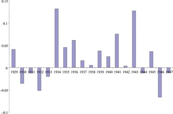
The various approaches pursued within the DSGE umbrella have had mixed success in dislodging strong priors. As a consequence, historical narrative has come to take on a particularly important role in persuading those not already committed. A challenge for the RBC approach is to provide plausible historical narratives consistent with the periodic and often substantial declines in TFP associated with recessions. Variations in the arrival rate of innovations might account for alterations in a positive rate of growth of TFP, but it is more difficult to see how such variations would periodically cause it to go negative.Footnote ³¹ Data for the years 1890 through 2004 indicate an average annual rate of private nonfarm TFP growth of 1.46 percent with a standard deviation of over 4 percentage points. There are many years in which TFP didn't just grow more slowly, it declined, often sharply (see Figure 1).

FIGURE 1

TFP GROWTH RATES, UNITED STATES, PRIVATE NONFARM ECONOMY, 1929–1947

Source: See source note for Table 1.

For 1948 and earlier, average annual TFP growth was 1.7 percent per year and the standard deviation was 5.4 percent. TFP declined in 23 of the 58 years: 1893, 1894, 1896, 1898, 1902, 1904, 1907, 1908, 1910, 1912, 1914, 1917, 1920, 1922, 1925, 1927, 1930, 1931, 1932, 1933, 1944, 1946, and 1947. On the face of it, it seems unlikely that all of these declines can be attributed to negative technological shocks or, absent that, innovations in bad government supply-side policy, with the implied counterfactual that within a minimalist state they would not have occurred.

The three most serious twentieth century output gaps developed in 1929–1933, 1974/75, and 1979–1982. In each of these episodes, TFP declined sharply. The most striking and problematic declines prior to the Second World War took place in 1930, 1931, 1932, and 1933 in the context of the worst output shortfall in U.S. economic history. Twelve percentage points of the more than 30 percent drop in real output between 1929 and 1933 is attributable to downward movement in TFP.

Although there is much we do not understand about what happened between 1929 and 1933, we do have well-established narratives detailing the effects of collapsing banks, a shrinking money supply, the interactions of debt and deflation, and plummeting velocity due to declines in spending on consumer durables and investment goods.Footnote ³² These accounts differ in terms of their relative emphasis on national and international factors, or on monetary vs. velocity shocks, but they reflect a shared view that the Great Depression was principally the consequence of aggregate demand shocks.

Ohanian has suggested that a meeting with President Hoover in November of 1929 persuaded industrialists to maintain high nominal (and thus, in the context of deflation), real wages in manufacturing, and that this explains part of the shrinkage in that sector through 1931.Footnote ³³ Much of the decline in manufacturing took place in durables. There is considerable evidence that overextended, overindebted, and uncertain consumers cut back sharply on this category of their spending.Footnote ³⁴ To this can be added the decline in orders attributable to the drop in the producer durables portion of investment expenditure.Footnote ³⁵ These demand-side shocks were the primary cause of the drop in manufacturing up through the banking crisis of October 1931. At issue here are not increases in nominal wages from prior levels, but rather their persistence; the actions or inactions of manufacturing wage setters should not therefore be considered a shock to the system. At best, a failure of nominal wages to decline faster can be seen as an institutional factor contributing to the non-neutrality of a negative aggregate demand shock.

Moreover, a more rapid decline in nominal wages in manufacturing—Ohanian's posited counterfactual—would have worsened the debt deflation problem. There is little in the modeling to capture the threat posed to output and employment by deflation in a world in which most borrowing and lending involved instruments with fixed nominal repayment obligations. There are many institutional features of an economy that can contribute to non-neutrality, and, as historical and contemporary experience indicates, the most significant of these may lie in financial as opposed to labor markets.

The other shocks emphasized by Cole and Ohanian, such as the National Industrial Recovery Act or the National Labor Relations Act, all took place after 1933, during a period of very rapid TFP growth (see Figure 1). They might possibly account for why TFP growth wasn't even faster after 1933, but they could not have played a role in the cumulative 12 percent decline in TFP under President Hoover.

There are well-known historical instances in which large declines in output can plausibly be linked to negative supply shocks. Russian/Soviet GDP and, presumably, TFP, declined sharply after 1913 and did not reattain its prewar level until 1926. But a historical narrative can point to large negative shocks, including the disastrous participation of the Russians in the First World War, the Treaty of Brest-Litovsk (which reduced Russian territory), the March 1917 Revolution, the October 1917 Bolshevik revolution, the Civil War between the Reds and the Whites, foreign intervention, and the political turmoil associated with the death of Lenin and the rise of Stalin.Footnote ³⁶ We lack any comparable supply-side narrative for the productivity declines during the worst years of the Great Depression in the United States.

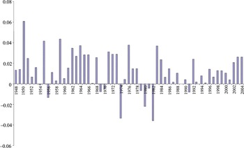
For the 1948–2004 period, average TFP growth is lower and less variable. The mean growth rate was 1.4 percent with a standard deviation of 1.8 percent. The reduced cyclical volatility of TFP during this period is arguably because cycles were weaker, at least between the 1982 recession and the 2007–2009 downturn. In the quarter-century prior to 2008, the U.S. economy experienced only two relatively minor recessions. Even with a lower ratio of standard deviation to mean, however, the level of TFP, not just its rate of growth, declined in 1954, 1956, 1969, 1970, 1974, 1979, 1980, 1981, 1982, and 1991 (see Figure 2).

FIGURE 2

TFP GROWTH RATES, UNITED STATES, PRIVATE NONFARM ECONOMY, 1948–2004

Source: See source note for Table 1.

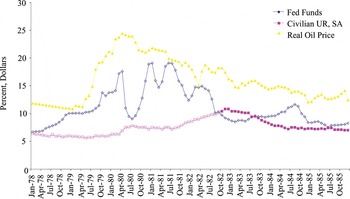
For the second half of the twentieth century, the largest output gaps developed in 1974/75 and 1979–1982. TFP declined in 1974 by 3.3 percent, and by .7 percent in 1979, 2.2 percent in 1980, .4 percent in 1981, and 3.6 percent in 1982.Footnote ³⁷ In contrast to the Depression years, there is a possible source of negative supply shocks, particularly between 1972 and 1985, that might have contributed to output retardation or decline during these episodes. Sharp increases in the price of oil resulting from decisions made by the Organization of Petroleum Exporting Countries produced deteriorations in the efficiency of the machine (foreign trade) whereby the United States transformed wheat, soybeans, plywood, and aircraft into oil. Prior to mid-century, when the United States was still the world's largest oil producer, oil shocks are of little relevance in understanding the aggregate economy. And, in part because of controls, there is relatively little change in the real price of a barrel of crude oil from the end of the Second World War through 1970. Between December 1973 and January 1974, however, that price more than doubled as a direct consequence of OPEC actions. And in April of 1979, the price again began rising rapidly. Following a peak in April of 1980, at which point it had more than doubled from a year earlier, it then began a steady decline before bottoming out in 1985. Aside from a brief spike during the first Gulf War, the real price of oil then remained relatively steady until after 2005.

It is commonly argued that, in contrast with 1980 or 1981/82, the 1974/75 recession was made in Vienna and Riyadh, not Washington. Still, the Federal Reserve, which had kept the Federal Funds rate under 5 percent as late as September 1972, allowed the rate to more than double over the next ten months. It remained above 10 percent between July 1973 and November of 1973 and then again between April and October of 1974. The discount rate, a less accurate measure of monetary tightness but a signal of Federal Reserve intentions, was raised in a series of steps from 4.75 percent in February of 1971 to 7.5 percent in August of 1973 to a peak of 8 percent in April of 1974. The role that monetary stringency played in inducing this recession has been perhaps underplayed. It was clearly implicated in the decline in investment spending which marked this downturn as well as so many others.

The NBER identifies the six months between January and July of 1980 and the sixteen months between July 1981 and November of 1982 as recessions. The proportional increase in the real price of oil was actually larger in 1979/80 than between December of 1973 and January of 1974. But its disruptive impact was less because, as a consequence of the first oil price shock, the U.S. economy had begun moving towards a more energy-efficient capital stock. A review of the sequence of oil price, interest rate, and unemployment rate movements between 1979 and 1982 helps explain why, in spite of the second oil price shock, the recessions of 1980 and 1981/82 are almost universally attributed to changes in aggregate demand conditions resulting from the tightening of monetary policy to fight inflation.

Even before the real price of oil began its yearlong upward movement in April of 1979, the Federal Funds rate began a climb into historically unprecedented territory. Following the seven-month period in 1974 when it had exceeded 10 percent, the rate declined to a trough in January of 1977 at 4.71 percent, then began a gradual upward movement. In December of 1978 it broke 10 percent again, hit 11.4 percent in September of 1979, and then 13.8 percent in October, when Chairman Volcker announced a new monetary regime in which the Fed would target monetary aggregates, and allow the funds rate to seek its own level. By April of 1980 the rate had increased to an eye-popping 17.6 percent (see Figure 3).

FIGURE 3

REAL OIL PRICE, FEDERAL FUNDS RATE, AND THE CIVILIAN UNEMPLOYMENT RATE, 1978–1985

Sources: Monthly Real Oil Price. St. Louis Federal Reserve Bank, “Spot Oil Price.” Deflator is CPI-U, Seasonally Adjusted, 1982–1984 =100 from U.S. Bureau of Labor Statistics, “Consumer Price Index.” Plotted data are half the values in 1982–1984 dollars. Federal Funds rate: St. Louis Federal Reserve Bank, “Federal Funds.” Left-hand scale is percent. Civilian Unemployment rate, seasonally adjusted: U.S. Department of Labor, “Employment Status.” Left-hand scale is percent.

Unemployment began to rise sharply, from 6.3 percent in March of 1980 to a peak of 7.8 percent in July. Concerned that the unprecedented monetary stringency would take the real economy into a major recession, the Fed relented, slashing the funds rate by almost half to a low of 9 percent in July of 1980. In reaction to monetary easing, the unemployment rate stopped rising, and remained in a range of 7.2–7.6 percent through September of 1981.

In the meantime, however, reconsidering the impact of its easing on inflationary expectations in both the bond and labor markets, the Fed again allowed the funds rate to move upward. It reached a new and unprecedented peak of 19.1 percent in January of 1981. The rate dropped to 14 percent in April but then rose again to 19.1 percent in June.Footnote ³⁸ In July of 1981 the unemployment rate began a relentless year and a half rise to a peak of 10.8 percent in November and December of 1982, as of this writing still the highest unemployment rate experienced since the Great Depression.

Economists such as Robert Lucas, a pioneer of rational expectations theory, predicted that we could have costless disinflation but were proved wrong. The rise in the unemployment rate from 7.2 percent in July of 1981 to its peak of 10.8 percent a year and a half later can't be attributed to negative supply shocks. The real price of oil had been declining steadily since April of 1980. Yet we continue to observe the declines in the level of TFP (not just its rate of growth) characteristic of recession.

With the possible exception of 1974/75, the most serious economic downturns of the twentieth century were precipitated by aggregate demand shocks and marked by negative TFP growth. The most plausible explanation for TFP declines during these periods is that demand shocks widened the output gap, and as the output gap widened, output fell, while capital input and cost largely didn't.