

Introduction
County-level health measures of mortality and morbidity are becoming more easily available and are being widely used by public health practitioners to track population health (Community Health Rankings & Roadmaps: A Healthier Nation, County by County 2012). One summary measure of general health, self-rated health status, is very common in both health-oriented and non-health-oriented surveys, and is also a foundational health measure in Healthy People 2020 (U.S. Department of Health and Human Services, 2011). However, to our knowledge, there has been no examination to date as to whether this indicator is responsive to changes in the amount of services provided by county departments of public health as measured by public health expenditures per capita.
While no current measure of general health status fully satisfies all of the criteria for the comprehensive measurement of health (Thacker et al., Reference Thacker, Stroup, Carande-Kulis, Marks, Roy and Gerberding2006), self-rated health status captures a great deal of information about an individual’s health and, in aggregate, population health. Self-rated health status has been found to predict disability, morbidity, mortality and other illness (Idler et al., Reference Idler, Russell and Davis2000; DeSalvo et al., Reference DeSalvo, Bloser, Reynolds, He and Muntner2006; Jyhlä, Reference Jyhlä2009; Rutledge et al., Reference Rutledge, Linke, Johnson, Bittner, Krantz, Whittaker, Eastwood, Eteiba, Cornell, Pepine, Vido, Olson, Shaw, Vaccarino and Bairey Merz2010; Pietiläinen et al., Reference Pietiläinen, Laaksonen, Rahkonen and Lahelma2011; Bopp et al., Reference Bopp, Braun, Gutzmiller and Faeh2012). Self-rated health status has also been shown to be significantly associated with factors that affect health such as sleep duration, obesity, social connections and hypertension labeling (Okosun et al., Reference Okosun, Choi, Matamoros and Dever2001; Barger and Muldoon, Reference Barger and Muldoon2006; Imai et al., Reference Imai, Gregg, Chen, Zhang, de Rekeneire and Williamson2008; Prosper et al., Reference Prosper, Moczulski and Qureshi2009; Zhang and Ta, Reference Zhang and Ta2009; Shankar et al., Reference Shankar, Charumathi and Kalidindi2011). In addition, trends in self-rated health status have been examined as a way to describe the evolution of health inequalities (Clarke and Ryan, Reference Clarke and Ryan2006).
The consistency of self-rated health across annual national health surveys is instructive regarding the reliability of this measure. The two annual national health surveys in the United States are the National Health Interview Survey (NHIS) and the Behavioral Risk Factor Surveillance Survey (BRFSS). Other surveys include sections on health, but these are the only two annual national health surveys in the United States that are focused on health. A major difference between these two surveys is one of question order. The NHIS asks about a large number of specific health conditions before the self-rated health item occurs. In contrast, the BRFSS only asks questions related to sampling before the self-rated health item occurs. Studies of the impact of question order on responses to self-reported health status items find that, among English speakers, asking the self-reported health status item after questions on specific health conditions, which can be seen as a form of self-education on the specifics of the respondent’s own health, results in either no impact or a slightly positive effect on self-reported health status (Crossley and Kennedy, Reference Crossley and Kennedy2002; Bowling and Windsor, Reference Bowling and Windsor2008; Lee and Grant, Reference Lee and Grant2009; Badawi et al., Reference Badawi, Gariepy and Schmitz2012). Thus, we expect that we may find a small shift between the NHIS and the BRFSS, with the NHIS reporting slightly higher levels of health with otherwise similar trends.
Figure 1 shows that this is exactly what occurs. Figure 1 presents a comparison of the time trends in these two surveys from logistic regressions where self-rated health is dichotomized into ‘good, very good or excellent health’ (healthy) vs ‘fair or poor health’ (unhealthy). Basic demographic controls are included for age (18–24, 25–34, 35–44, 45–54, 55–64, 65–74, 75 and higher), sex, race/ethnicity (white, black, Hispanic, other), marital status (married, single, divorced/separated, widowed) and education (less than high school, high school, any college, college graduate and higher). The vertical axis represents the marginal probabilities of being healthy in a given year (relative to 1996), controlling for the above sociodemographics, while the horizontal axis represents years. The two surveys appear to largely mirror each other, particularly during the 2001–2009 periods that we are interested in, with the NHIS trends being consistently higher than those of the BRFSS, as expected.
Comparison of General Health Status Trends in Annual US National Health Surveys. NHIS: National Health Interview Survey; BRFSS: Behavioral Risk Factor Surveillance Survey. Figure based on logistic regressions controlled for age, sex, race, education and marital status. NHIS data come from the Integrated Health Interview Series (2012).

However, the sample sizes of the NHIS and the BRFSS are too small to obtain statistically valid county estimates of self-rated health. Thus, this study uses a state health survey with a question order similar to that of the BRFSS, but which is specifically designed to provide statistically valid estimates at the county level over a relatively long period of time: the California Health Interview Survey (CHIS). The CHIS is also more reliable than the either the NHIS or the BRFSS in its state-level estimates, given its much larger sample size and county stratification.
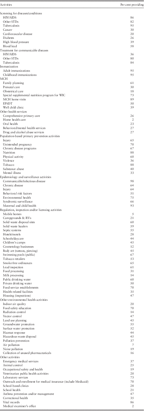
What patterns might we expect between per capita county public health expenditures and county-level population health status over time? Table 1 presents the activities of county departments of public health in California.Footnote 1 Spending on some of the activities listed, such as influenza immunizations, treatment for communicable diseases, disease screening, prenatal care, regulating public drinking water, regulating food service establishments and others, will clearly have immediate effects on the health status of many individuals and thus, the health status of the population. Other activities, such as population-based prevention activities, will take a longer period of time to impact the health status of individuals. Thus, the impact of any given year of public health expenditures will not only affect the health status of the population in the year the activities funded by public health expenditures were performed, but will also affect the health status of the population for years to come. Any analysis that hopes to capture the relationship between public health expenditures and health status must therefore be able to account for the cumulative impact of public health expenditures on the health status of the population over time.
Activities of California county departments of public health
MCH=maternal and child health; WIC=women, infants and children; EPSDT=Early and Periodic Screening, Diagnosis, and Treatment.
Source: 2010 National Profile of Local Health Departments
Previous research examining the relationship between county-level expenditures and health has primarily focused on mortality, and finds that county-level mortality rates, both all-cause and disease specific, are reduced when expenditure levels of county departments of public health rise (Grembowski et al., Reference Grembowski, Bekemeier, Conrad and Kreuter2010; Erwin et al., Reference Erwin, Greene, Mays, Ricketts and Davis2011; Mays and Smith, Reference Mays and Smith2011; Brown, Reference Brown2014). However, of these studies, only Brown (Reference Brown2014) has attempted to measure cumulative impact. To our knowledge, the current study is the first to estimate the impact of changes in per capita county public expenditures on county-level general health status, where cumulative impact is taken into account.
Methods
Conceptual and econometric model
The causal link between per capita county public health expenditures and county-level self-rated health is placed in the context of an aggregate demand for health model. We define an aggregate demand for health model is an aggregate version of the individual demand for health model where health status is a function of the price of medical care, income, age, education and variables affecting preferences for health, such as race/ethnicity (Zweifel and Breyer, Reference Zweifel and Breyer1997). As decision making regarding county department of public health expenditures occurs at the county level, the county is used as the unit of analysis.
As noted above, the main hypothesis is that the key variable of interest, per capita county public health expenditures, will positively affect the health status of the population, both contemporaneously and in the future. While it is possible to reformulate the hypothesis to whether per capita county public health expenditures will positively affect the health status of the average individual in the population (as opposed to the health status of the overall population) contemporaneously and in the future, the necessary econometric model, which uses a lagged dependent variable, would require individual-level panel data. Individual-level panel data are not available, therefore the hypothesis is formulated at the population level and available county-level panel data are used.
A standard Koyck distributed lag model is estimated, which assumes that the effect of county public health expenditures is cumulative (Wooldridge, Reference Wooldridge2003). The cumulative impact is the sum of a contemporaneous impact, and any subsequent future impacts, which are assumed to decline geometrically over time as it may take longer periods of time for some programs to create measureable impacts on individuals with higher levels of health status and the impacts of such programs on individuals with higher levels of health status are likely to be smaller (Bopp et al., Reference Bopp, Braun, Gutzmiller and Faeh2012). In other words, the cumulative impact of public health expenditures becomes larger over time, but at a declining rate.
The Koyck model can be described as follows:
 $${\rm y}_{t} ={\rm \alpha }{\plus}\beta _{0} x_{t} {\plus}\beta _{1} \lambda x_{{t{\minus}1}} {\plus}\beta _{2} \lambda ^{2} x_{{t{\minus}2}} {\plus}\cdots{\plus}u_{t} ,$$
where y is the percentage of individuals who rate their health as good, very good or excellent on a five-level health status item (poor, fair, good, very good, excellent), x is county public health expenditures per capita, and λ, where 0<λ<1, is the estimated rate of change of the distributed lag. The number of lags included in the model is theoretically infinite, but practically, the number of relevant lags depends on the size of λ. Larger values of λ yield lag structures where relatively large coefficients are present further and further back in time (in other words, the impact of public health expenditures is substantial for a longer period of time in the future). Additional parameters to be estimated are represented by α and β. Finally, u t is the error term. To simplify, we lag equation (1) by one period, multiply it by λ, subtract this lagged equation from equation (1), and then rearrange:
 $$y_{t} =\alpha _{0} {\plus}\beta _{0} x_{t} {\plus}{\rm \lambda }y_{{t{\minus}1}} {\plus}v_{t} ,$$
where v t=(u t−λu t−1) and α 0=α(1−λ). Other public-health researchers have also taken a dynamic approach in recent research (Macinko et al., Reference Macinko, de Oliveira, Turci, Guanais, Bonolo and Lima-Costa2011). The cumulative or long-run impact can be determined by substituting long-run values of both county-level general health status and per capita county public health expenditures into the above equation. We define y* as the long-run value of y and x* as the long-run value of x. Substituting these values into equation (2) yields the following equation:
 $$y^{\asterisk}=\alpha _{0} {\plus}\lambda y^{\asterisk}{\plus}\beta x^{\asterisk}.$$
We then solve for y*:
 $$y^{\asterisk}=\alpha _{0} /(1{\minus}\lambda ){\plus}[(\beta )/(1{\minus}\lambda )]x^{\asterisk}.$$
To determine the long-run cumulative impact of increasing (or decreasing) per capita county public health expenditures, we take the first derivative with respect to x*:
 $${{\partial y^{\asterisk}} \over {\partial x^{\asterisk}}}=\beta /(1{\minus}\lambda ).$$
Many readers will recognize this as the standard result for the sum of an infinite geometric series where 0<λ<1. This can also be referred to as the long-run propensity (LRP; Wooldridge, Reference Wooldridge2003). The short-run propensity (SRP), or initial impact, can be defined as β alone.
In order to be empirically estimated, equation (2) must be adjusted in order to include standard factors relevant to the aggregate demand for health. As noted above, these include the price of medical care, income, age, education and factors that influence population preferences for health, such as race/ethnicity. Prices of medical care can be proxied using the proportions of the population covered by health insurance including Medicaid and related programs, Medicare, and private health insurance. Income is measured as per capita income. Age is measured by the age structure of the population (proportion of the population in the following ranges: 0–14, 15–24, 25–34, 35–44, 45–54, 55–64, 65–74, 75–84, 85 and older). Education is measured by the extent to which the population has a college education, which is measured by the proportion of the population who have a bachelor’s degree or higher. The racial/ethnic structure of each county’s population is measured by the proportion of individuals in each racial/ethnic group (White, Black, Hispanic, Asian/Pacific Islander, Other).
None of the variables used in the analysis are age-adjusted. We follow the approach of Rosenbaum and Rubin (Reference Rosenbaum and Rubin1984), who note that when using an age-adjusted population rate as a dependent variable in regression analysis, all independent variables must also be age-adjusted in order to avoid biased parameter estimates. When age-adjusted variables are not available for every variable in the model, they show that using crude population rates for both the dependent and independent variables, while adjusting for age by including variables indicating the proportion of the population in each age category, will yield consistent estimates.
We include per capita public health expenditures to complete the description of the institutional context. County health expenditures in California are formally categorized into four reporting categories (public health, medical care, drug and alcohol abuse and mental health). Note that these categories all represent health expenditures that flow through each county government. Because each of these is endogenous in our model (at least subject to omitted variable bias and measurement error), we only include public health expenditures following Angrist and Pischke (Reference Angrist and Pischke2009) who recommend omitting uncorrected endogenous variables in instrumental variables equations. All control variables (health insurance, income, age, education, race/ethnicity) in the model are lagged in order to render all control variables strictly exogenous or weakly exogenous (predetermined).
Two variables in the model are endogenous to the percentage of the population reporting good, very good or excellent health: the lagged dependent variable and per capita county public health expenditures. The main aspects of endogeneity with regard to per capita county public health expenditures are omitted variable bias and measurement error. For example, the equation does not contain information on varying health policy ordinances, varying environmental conditions, varying population health behaviors, or other factors that may correlate with both self-rated health and county public health expenditures. See the ‘Discussion’ section below regarding per capita county public health expenditures being measured with error. These two endogenous variables, the lagged dependent variable and per capita county public health expenditures, can be handled in at least three ways. One is through standard instrumental variables. However, standard instrumental variables are often unavailable or too weak. In these cases, at least two alternative approaches are available. One is the generalized method of moments (GMM) system estimator, which is designed for panels with a small number of time periods and a large number of observations within each time period where it is not assumed that adequate instruments are available outside of the core data set (Roodman, Reference Roodman2009). However, if the available valid instruments (lagged levels and lagged differences) used by the GMM system estimator (Blundell and Bond, Reference Blundell and Bond1998) are weak, the result can be significant parameter bias, similar to that found in traditional instrumental variable models with weak instruments (Bun and Windmeijer, Reference Bun and Windmeijer2010). Only ad-hoc methods of testing for weak instruments are currently available when using the GMM system estimator (Bazzi and Clemens, Reference Bazzi and Clemens2013).
An alternative approach that allows traditional weak instrument testing and also does not require outside instruments is that of Lewbel (Reference Lewbel2012). Lewbel’s approach was disseminated through working papers before publication resulting in a large number of studies being published that applied Lewbel’s methodology both before and after the formal publication of Lewbel’s methodology (Stifel and Alderman, Reference Stifel and Alderman2006; Block, Reference Block2007; Sabia, Reference Sabia2007a, Reference Sabia2007b, Reference Sabia2007c; Haung et al., Reference Huang, Lin and Yeh2009; Kelly and Markowitz, Reference Kelly and Markowitz2009; Drichoutis et al., Reference Drichoutis, Nayga and Lazaridis2012; Emran and Shilpi, Reference Emran and Shilpi2012; Kelly et al., Reference Kelly, Dave, Sindelar and Gallo2012; Lewbel, Reference Lewbel2012; Denny and Oppedisano, Reference Denny and Oppedisano2013; Huang and Xie, Reference Huang and Xie2013; Schroeter et al., Reference Schroeter, Anders and Carlson2013).
Lewbel (Reference Lewbel2012) uses any heteroscedasticity present in the data to generate sets of valid instruments. Lewbel’s approach does not identify the endogenous variables in the second-stage equation based on traditional exclusion restrictions. Rather, he achieves identification using higher moments. Sufficient conditions for Lewbel’s method to be applied are as follows:  $$Cov(Z,{\varepsilon}_{1} {\varepsilon}_{2} )=0$$
,
 $$E(X{\varepsilon}_{1} )=0$$
, and
 $$E(X{\varepsilon}_{2} )=0$$
, where Z is a subset of X, the vector of exogenous variables in the second stage (and Z may include all of X) along with some heteroscedasticity in
 $${\varepsilon}_{1} $$
and
 $${\varepsilon}_{2} $$
, the errors from both the first and second stages of a standard IV regression. As noted by Lewbel (Reference Lewbel2012), a standard overidentication test can be used to evaluate the validity of these assumptions.
Potentially valid instruments are constructed by multiplying the heteroscedastic residuals from the first-stage regressions with a subset (or all) of the mean-centered exogenous variables $$(Z{\minus}\bar{Z})\hat{{\varepsilon}}_{1} $$
, where
 $$\hat{{\varepsilon}}_{1} $$
is the vector heteroscedastic residuals from the first-stage regressions and
 $$\bar{Z}$$
is a vector of the means of Z.
These generated instruments may be weak or strong, depending on the degree of scale-related heteroscedasticity in the data. Heteroscedasticity can be detected using a standard Breusch–Pagan type test (Lewbel, Reference Lewbel2012). The strength of the generated instruments can be evaluated using standard weak instrument tests (Stock and Yogo, Reference Stock and Yogo2005). As this approach may produce a mix of strong and weak instruments, it is valuable to remove weak instruments from the set of instruments used. The approach taken here is to remove instruments as needed if the absolute value of the instrument’s t-statistic is <1.96 in both of the first-stage regressions.
A final point is that when using panel data, two independent panels can be spuriously associated if they both have unit roots (Granger and Newbold, Reference Granger and Newbold1974; Wooldridge, Reference Wooldridge2003). We therefore test for the existence of unit roots using a test that assumes that the number of units, N, can be constant, as counties are unlikely to be added to California. In particular, we perform Phillips–Perron (Reference Phillips and Perron1988) tests, which use Newey-West (Reference Newey and West1987) standard errors to account for any serial correlation. The null hypothesis is that the data follow a random walk with or without drift. We use the z-statistic as our test statistic, which is recommended by Choi (Reference Choi2001) as offering the best trade-off between size and power. Following the recommendation of Levin et al. (Reference Levin, Lin and Chu.2002), all series are first demeaned by subtracting the cross-sectional means to mitigate the influence of cross-sectional dependence.
All analyses are performed using Stata 11 and ivreg2 using two-step feasible GMM estimation and ordinary least squares (OLS) for comparison purposes (Baum et al., Reference Baum, Schaffer and Stillman2010; Lewbel, Reference Lewbel2012). After generating IVs from non-clustered, heteroscedastic regressions, we cluster our data by county to correct for any downward bias in the standard errors from the presence of any serial correlation following the suggestion of Angrist and Pischke (Reference Angrist and Pischke2009). Petersen’s (Reference Petersen2009) work on panel data also suggests clustering by county to avoid biasing the standard errors when seeking to take into account both the correlation of observations within clusters and the correlation of observations within time periods, with the latter being taken into account parametrically (by including time dummies). The cumulative impact of county-level per capita public health expenditures is then estimated by evaluating the overall non-linear combination of [ $$(\beta _{0} )/(1{\minus}\lambda )$$
] from equation (5).
Data
Self-rated health status at the county-level comes from the California Health Interview Survey (CHIS), which is fielded biennially. Health status is measured from high to low in five categories as excellent, very good, good, fair and poor. Categories are collapsed in accordance with the common practice of dichotomising the variable into two categories: poor/fair and good/very-good/excellent. Thus, the county-level measure is the percentage of individuals in the county with good, very good or excellent health status.
Information on the per cent of the population with Medicaid or other public insurance, the per cent of the population with Medicare, per cent of population with private insurance and the per cent of the population with a bachelor’s degree or higher also come from the CHIS. The CHIS is designed to yield statistically valid county-level measures for 41 of California’s 58 counties. The survey incorporates large statistically valid samples in each county from all age groups including children, teens and adults. However, subsetting self-rated health status by race/ethnicity was not feasible as sample sizes then became small and statistically unstable in many counties. For this reason subgroup analysis by race/ethnicity was not performed.
Data were obtained on county-level expenditures for public health from the 2001, 2003, 2005, 2007 and 2009 versions of the Counties Annual Report issued by the California State Controller’s Office. The Counties Annual Report details county expenditures, including public health expenditures (California State Controller’s Office, 2011). The report separates county health expenditures into four categories: public health, medical care, mental health and drug and alcohol abuse. It is not possible to disaggregate county health expenditures further using this report. The determination of how services are categorized across these four classes is a county decision and not all counties categorize services in the same way. Thus, county public health expenditures are subject to some degree of measurement error.
San Francisco, the only county in California that is also a city, is included in the Counties Annual Report, but is accorded a separate appendix due to its combined city-county functions. Because of its unique organizational structure, its expenditures are difficult to compare with the expenditures of other counties. It was therefore omitted from the analysis. The remaining 40 out of 58 counties represent ∼96% of the population of California.
The proportions of the population in nine age groups (0–14, 15–24, 25–34, 35–44, 45–54, 55–64, 65–74, 75–84, 85 and older) and in five racial/ethnic categories (White, Black, Hispanic, Asian/Pacific Islander and other race) come from the US Census (RAND, 2012). Per capita income comes from the US Bureau of Economic Analysis. All dollar figures are adjusted for inflation and reported in constant 2009 dollars. The analysis includes a total of 199 observations, 40 county-level observations for each year (with the exception of one county for which some data elements were unavailable for one year). The years included are 2001, 2003, 2005, 2007 and 2009.
Results
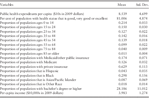
Table 2 presents descriptive statistics. There is a very large variation in our dependent variable both between counties and within counties. The per cent of the population reporting good, very good or excellent health status ranges from 68.7% to 90.7%. Within-county standard deviations range from 0.30% to 5.63% with a median of 1.7% showing that there is plenty of movement in general health status within counties for the model to capture.
Descriptive county-level statistics: 2001, 2003, 2005, 2007, 2009 (n=199)
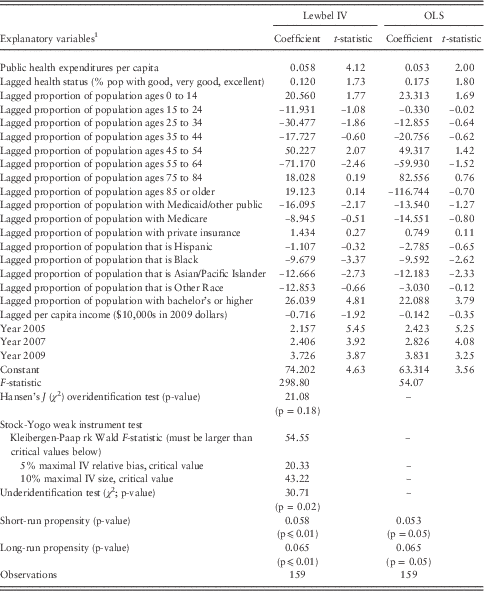
Table 3 presents the results of the Lewbel instrumental variable (IV) dynamic panel model and the same dynamic panel model estimated using ordinary least squares. A precondition of either model is that each variable in the model does not have a unit root. For every variable in the model, Phillips–Peron tests rejected the null hypothesis that every panel contained a unit root (p⩽0.05). An initial estimation of the Lewbel IV model was performed and all instruments were removed where the t-statistic was <1.96 in both of the first-stage regressions. This was sufficient to reject underidentification and weak instruments in the second stage, with the overidentification test not rejecting instrument exogeneity. However, in order for the estimated covariance matrix of moment conditions to achieve full rank in the first-stage regressions, one additional instrument needed to be removed. The final Lewbel IV model shows that the null hypothesis of model underidentification is rejected (χ 2=30.71, p=0.02), the null hypothesis of weak instruments is rejected (Kleibergen-Paap rk Wald F-statistic=54.55, which is larger than the critical value for 5% maximal IV relative bias, 20.33, and larger than the critical value for 10% maximal IV size, 43.22), but the null hypothesis that the identifying instruments are exogenous (overidentification test) is not rejected (χ 2=21.08, p=0.18). The model is statistically valid.
Aggregate demand for health: distributed lag model
1Note that one age category (ages 65–74) one insurance category (uninsured), one education category (less than bachelor’s degree), one racial/ethnic category (proportion of the population that is White, and one year category (year 2003), are omitted to avoid perfect multicollinearity.
However, the OLS model yields very similar results indicating that the OLS model is not severely affected by the biases that the instrumental variable model was intended to correct. In both models, most of the impact on general health status occurs in the year that funds are expended, with a small residual occurring across future years. Both models suggests that, over the long run, a $10 increase in per capita county public health expenditures in a given year would increase the percentage of the population reporting good, very good or excellent health by 0.065 percentage points. This annual increase in an annual expenditure cycle would impact ∼24,015 individuals across the 40 counties. Assuming no diminishing returns in the relationship between county public health expenditures and health status, county public health activities funded at current levels improve the health status of ∼0.56% of the population (0.56=0.065×8.539) with each annual expenditure cycle impacting ∼207,000 individuals (0.0056×36,945,637 estimated population in 40 counties in 2009). If diminishing returns are present, this is an underestimate.
In both models, higher concentrations of Blacks and Asian/Pacific Islanders were associated with lower population health. This is consistent with California individual-level estimates that show that both Blacks and Asian/Pacific Islanders are more likely to report poor or fair health relative to Whites (California Health Interview Survey, 2011). In contrast, both models found that higher rates of college education (bachelor’s or higher) were associated with greater population health, consistent with major findings in the literature on the individual-level relationship between education and health (Eide and Showalter, Reference Eide and Showalter2011). Finally, an upward trend in general health status was also apparent, on average, across these 40 counties. Note that, when considering the associations of the control variables with the dependent variable, the relationships found in county-level models will often be different from the relationships that would be found in individual-level models. This is known as the aggregation problem in econometrics (also called the ecological fallacy problem in sociology; Chan, Reference Chan2005). Only the instrumented relationships in the model are corrected for bias and these variables only measure aggregate relationships.
Discussion
We estimated the short-term and long-term effects of county public health expenditures on the percentage of the population reporting good, very good or excellent health status over a nine-year period (2001–2009) using a standard Koyck model of dynamic relationships. The main finding is that a long-term $10 annual increase in per capita public health spending in the 40 counties examined in California (representing 96% of the population) would move the health of ∼24,000 individuals from the ‘poor or fair’ category to the ‘good, very good or excellent’ category each year the increase was in place. The annual cumulative effect of current expenditure levels of county departments of public health is 207,000 individuals being in the ‘good, very good or excellent’ categories of health status rather than the ‘poor or fair’ categories.
The size of this impact is directly related to the proportion of the population that is primarily served by county departments of public health. The size of this proportion will vary depending on the population characteristics of a given county.
Although the cost of this change in population health may appear to be implied, the cost related to changes in general health status is also related to changes in mortality (Brown, Reference Brown2014). The relationship between per capita public health expenditures and mortality exhibits a much longer cumulative time period than the cumulative time period implied by the current model. This is actually quite consistent with the large literature that finds that changes in general health status tend to precede mortality (DeSalvo et al., Reference DeSalvo, Bloser, Reynolds, He and Muntner2006). It thus appears that the activities of county public health departments in California in a given year may initially impact the general health status of the population (having a cumulative impact on ∼207,000 individuals) and, over a longer time period (approximately a decade), decrease mortality in the population (∼26,000 deaths avoided; Brown, Reference Brown2014). This repeats each year. The extent to which those whose deaths are averted are the same individuals whose general health status was improved earlier is unknown at the current time, although we suspect that there is a very large overlap.
There are at least two limitations to this study. The first is that this study only examined movement between the combined set of the two lowest levels of general health status and the combined set of the three highest levels of general health status, and thus necessarily did not capture any relationship between per capita public health expenditures and positive movement within the set of the two lowest levels of general health status or positive movement within the set of the three highest levels of general health status.
An additional limitation to this study is that, although the time period used in this study was relatively long (almost a decade), it is possible that a longer time period may yield somewhat different results. For example, some spending on chronic disease prevention may not be fully reflected. This may affect the magnitude of the estimates.
Public health activities are of significant societal value and should be recognised as such. This study is one among many recent studies that are beginning to demonstrate this to the larger health policy community. The current study highlights the overall average effectiveness of public health activities in improving population health, but is unable to address important additional questions, such as what the most cost-effective bundle of public health services may be. In order to move in this direction, publicly available data on public health expenditures are needed where public health expenditures are disaggregated into more subcategories. In addition, publicly available information is needed on the various subpopulations that primarily receive services within each subcategory. Such information could be acquired by the state implementing specific reporting requirements, developed in cooperation with county public health departments. Movement in this direction would facilitate research to determine the county public health activities that are most cost-effective so that funding can be expanded in areas that are found to yield the best outcomes.
Acknowledgments
This research was funded by the Robert Wood Johnson Foundation, Grant No. 67617. The Robert Wood Johnson Foundation was fully independent and did not participate in the design, interpretation, writing or decision to publish this research. Gabriella Wong, M.P.H. and Anupriya Dayal participated by performing literature reviews.