1 Introduction
The dynamics of solid–liquid mixtures and slurries plays an important role in natural settings as well as environmental, process and biomedical engineering. The study presented here is motivated by the need for a fundamental understanding to support modelling of inertial flows of liquid–solid suspensions in general bounded geometries. It is well established that inertia may have a significant influence on particle motion, leading for example to heterogeneity in the spatial distribution of the particle concentration and to the modulation of transport properties (Haddadi et al. Reference Haddadi, Shojaei-Zadeh, Connington and Morris2014). We focus in this work on the case of inertial effects on the motion of a spherical particle in a flow with a strong wall-normal component, a case which has seen limited investigations so far.
We refer to fluid inertia at the particle scale, evaluated through the Reynolds number  $Re=2\unicode[STIX]{x1D70C}Ba^{2}/\unicode[STIX]{x1D707}$, where
 $a$ is the particle radius,
 $B$ is the characteristic strain rate of the flow and
 $\unicode[STIX]{x1D70C}$ and
 $\unicode[STIX]{x1D707}$ denote the fluid density and viscosity, respectively (hence the kinematic viscosity is
 $\unicode[STIX]{x1D708}=\unicode[STIX]{x1D707}/\unicode[STIX]{x1D70C}$). Particle inertia is intrinsically related to the particle response time, characterized by the Stokes number
 $St=(\unicode[STIX]{x1D70C}_{p}/\unicode[STIX]{x1D70C})Re/9$, with
 $\unicode[STIX]{x1D70C}_{p}$ the particle density. An early demonstration of the influence of inertia on the mixture properties was presented by Bagnold (Reference Bagnold1954), who showed that the stress in a neutrally buoyant suspension varies linearly with the shear rate,
 $\dot{\unicode[STIX]{x1D6FE}}$, at small rates, transitioning to a
 $\dot{\unicode[STIX]{x1D6FE}}^{2}$-dependence as the shear rate increases. Later, this work was criticized and bulk effects of particles at large inertia were reconsidered (Hunt et al. Reference Hunt, Zenit, Campbell and Brennen2002). To understand flows in arbitrary geometries, we must focus attention beyond parallel shear flows, e.g. Poiseuille or Couette flows, the study of which (Segré & Silberberg Reference Segré and Silberberg1962; Ho & Leal Reference Ho and Leal1976; Vasseur & Cox Reference Vasseur and Cox1976; Matas, Morris & Guazzelli Reference Matas, Morris and Guazzelli2004; Loisel et al. Reference Loisel, Abbas, Masbernat and Climent2015) has led to a well-developed characterization of inertial migration of particles, and to a better understanding of the modulation of flow turbulence by suspended particles (Matas, Morris & Guazzelli Reference Matas, Morris and Guazzelli2003; Shao, Wu & Yu Reference Shao, Wu and Yu2012; Wang, Abbas & Climent Reference Wang, Abbas and Climent2017; Zade et al. Reference Zade, Costa, Fornari, Lundell and Brandt2018). In other geometries, such as the flow around an obstacle or in a pipe bend, there are regions where the flow is incident onto a surface. While studies of gas–solid jets inducing surface erosion are known, for instance in turbo-machinery (Hamed, Tabakoff & Wenglarz Reference Hamed, Tabakoff and Wenglarz2006), liquid–solid mixtures impinging on an obstacle have rarely been considered, yet these are encountered in a number of applications, including slurry mixing with impellers (Cumby Reference Cumby1990), water ice-jet machining (Gupta et al. Reference Gupta, Avvari, Mashamba and Mallaiah2017), surface dust removal (Maynard & Marshall Reference Maynard and Marshall2012) as well as in river transport of sand past bridge pilings.
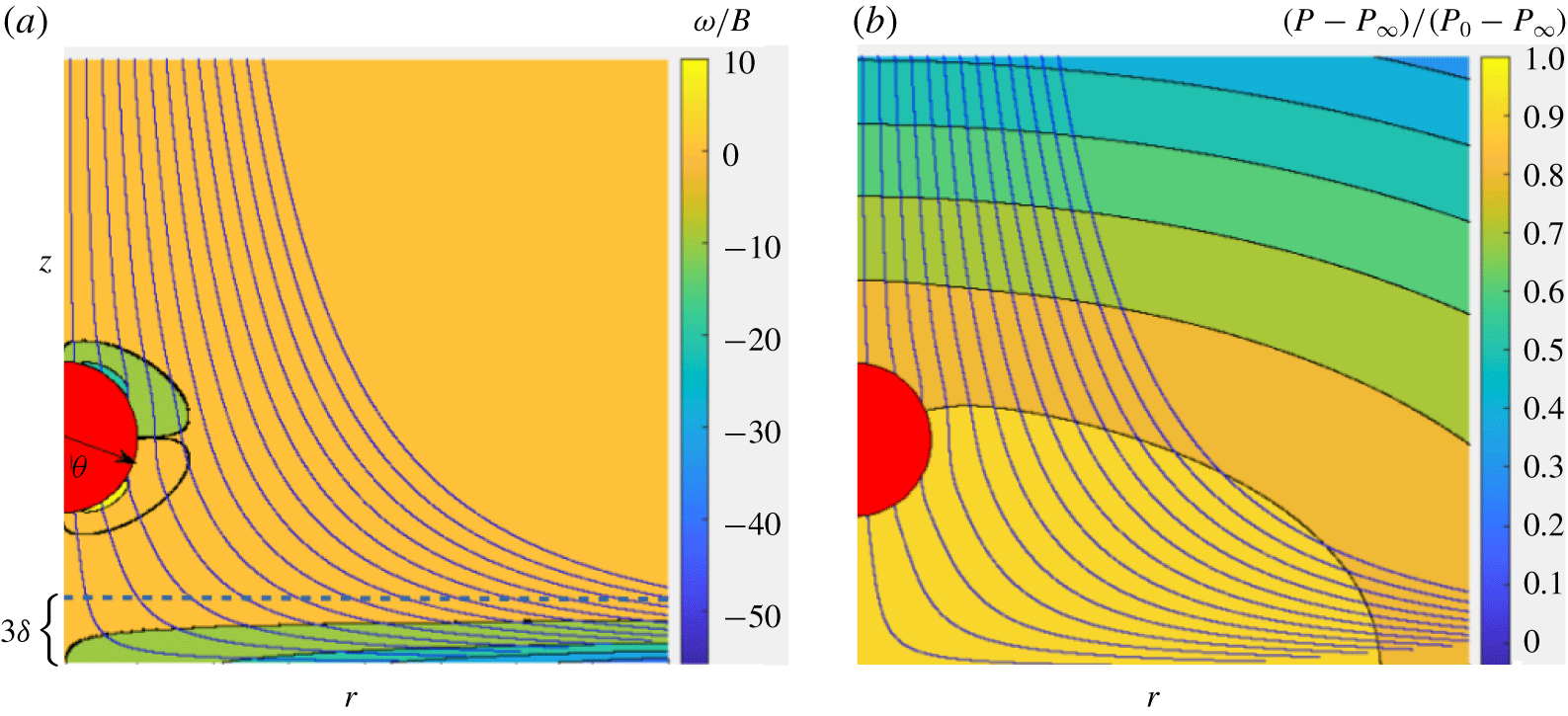
As a foundation for understanding suspension flows with wall-normal velocity, we investigate in detail the dynamics of a single sphere approaching a stagnation point on a flat and smooth wall, as shown schematically in figure 1(a). Here, the flow kinetic energy is converted into a pressure increase which decelerates the flow, as illustrated in figure 1(b). This is well described for the pure fluid motion by the well-known Hiemenz boundary-layer solution (Hiemenz Reference Hiemenz1911) and its axisymmetric counterpart, the Homann solution (Homann Reference Homann1936). The present study focuses on the latter base flow, abbreviated as Hiemenz–Homann or ‘HH flow’ throughout the paper. We find that, even for a neutrally buoyant particle, the particle is driven under inertial conditions to approach the wall more rapidly than expected under creeping-flow conditions. A natural question then arises as to whether this leads to necessary conditions for a particle–wall collision with rebound, a phenomenon that would have significant consequences for the boundary condition to be applied to continuum modelling of the mixture flow. Fluid mechanical analysis alone is not sufficient to ascertain whether collisions may occur or not, since the Navier–Stokes equations should be supplemented with wall surface properties (roughness and wetting characteristics). The problem studied here is similar in some respects to that encountered in studies of sphere rebound from a wall in an otherwise quiescent fluid, which is known to be controlled by particle inertia (Joseph et al. Reference Joseph, Zenit, Hunt and Rosenwinkel2001; Legendre et al. Reference Legendre, Zenit, Daniel and Guiraud2006) and particle–wall surface conditions, including the effect of surface roughness (Mongruel et al. Reference Mongruel, Lamriben, Yahiaoui and Feuillebois2010; Izard, Bonometti & Lacaze Reference Izard, Bonometti and Lacaze2014). However, we emphasize that the problem we study is qualitatively different, as the same net force acts on the rigid particle and the fluid particle of same volume sufficiently far from the wall.
Sketch of a rigid spherical particle transported on the axis of an axisymmetric HH flow, some streamlines of which are displayed. (a) Vorticity iso-levels (vorticity is scaled by the flow strain rate,  $B$); (b) pressure iso-levels (pressure differences with respect to the pressure at infinity,
 $P_{\infty }$, are scaled by the pressure difference at the stagnation point,
 $P_{0}-P_{\infty }$, determined in the single-phase HH flow). The outer edge of the boundary layer, where the radial fluid velocity component reaches 98 % of its free-stream value, stands a distance
 $3\unicode[STIX]{x1D6FF}$ from the wall.

In wall-normal flow, the relevant length scale close to the wall is set by the characteristic thickness of the boundary layer,  $\unicode[STIX]{x1D6FF}=\sqrt{\unicode[STIX]{x1D708}/B}$. Across this boundary layer, all velocity components decrease to zero to satisfy the no-slip condition at the wall. We consider a particle whose centre lies on the streamline that ends at the stagnation point of the axisymmetric straining flow. An extremely small particle on this particular streamline would slow down and asymptotically reach the stagnation point. However, a finite-size particle exhibits deviation from tracer motion even in Stokes flow, and the situation is considerably altered when inertia plays a role. For conditions where inertia is negligible, Goren & O’Neill (Reference Goren and O’Neill1971) and Rallabandi, Hilgenfeldt & Stone (Reference Rallabandi, Hilgenfeldt and Stone2017) established theoretically the balance of wall-normal forces experienced by a particle approaching a large obstacle, considering that the undisturbed flow varies quadratically with the distance to the particle centre. The lubrication resistance due to particle–wall interaction diverges as the gap (defined as the distance
 $h$ separating the wall from the point on the particle closest to it) becomes very small, which allows the velocity toward the wall driven by the external flow to tend to zero. At high Reynolds or Stokes numbers (large particle size or relative density), Vigolo et al. (Reference Vigolo, Griffiths, Radl and Stone2013) determined the finite impact and bouncing velocities of particles moving in a liquid near the stagnation point located at the bifurcation of a symmetric T-shaped junction. Their study was mostly concerned with particles denser than the fluid, although some cases approached neutral buoyancy. The particle trajectory equation based on a simple empirical model for the hydrodynamic forces (the sum of viscous drag, added mass, rotation-induced lift and lubrication effects) allowed reasonable prediction of the conditions yielding impact events.
When the particle size is such that  $a/\unicode[STIX]{x1D6FF}\sim \mathit{O}(1)$, a finite slip velocity (defined as the relative velocity between the particle and the undisturbed flow at the position of its centre) is expected near the wall, since the particle is rigid and stops with its centre apart from the wall, whereas an equivalent volume of fluid would deform continuously. In such a situation, the work of Vigolo et al. (Reference Vigolo, Griffiths, Radl and Stone2013) suggests that the particle approach to the wall is retarded and the rate of particle–wall collisions is reduced. Their approximate model of hydrodynamic forces agrees qualitatively with the measurements in the stagnation point region, but systematically over-predicts the particle impact velocity at the stagnation point. A theoretical prediction of the hydrodynamic forces in this flow configuration is challenging, since the inertial contribution to the stress distribution at the particle surface, outside the gap, may be important. Moreover, the viscous resistance may be insufficient to stop the particle against the fluid driving force, allowing the gap width to approach the roughness length scale of solid surfaces such that continuum fluid mechanics may break down in the gap.
The dynamics of a spherical neutrally buoyant finite-size particle in a wall-normal flow thus raises several fundamental open questions. Understanding the particle approach to the stagnation point in the range of large-to-moderate dimensionless gaps, say  $\unicode[STIX]{x1D716}=h/a\gtrsim 1$, is one of them, as little is known regarding viscous and inertial wall-induced hydrodynamic forces in this flow configuration. This state of affairs motivated a specific theoretical study reported elsewhere (Magnaudet & Abbas Reference Magnaudet and Abbas2020). In that work, viscous and inertial forces acting on a spherical particle moving near the stagnation point of a HH flow are predicted under restrictive conditions, especially
 $Re\lesssim 1$,
 $a/\unicode[STIX]{x1D6FF}\ll 1$ and
 $\unicode[STIX]{x1D716}\gtrsim 1$. Here, we are mainly interested in larger particles, especially in the transition from non-impacting conditions, where the motion is purely controlled by hydrodynamics, to impacting conditions, where continuum mechanics may break down, which is expected to occur for particles such that
 $a/\unicode[STIX]{x1D6FF}\sim 1$. Indeed, the surface of large particles such that
 $a/\unicode[STIX]{x1D6FF}\gtrsim 1$ may closely approach the wall while their centre still stands outside the boundary layer, as illustrated in figure 4. To address this range of conditions, we examine the particle dynamics in the HH flow using numerical simulation, the particle and fluid motions being coupled through an immersed boundary approach. The simulations are carried out using extremely refined grid distributions in the gap, in order to fully resolve lubrication effects; they are eventually stopped at very small gaps typical of roughness effects.
We pause to emphasize central points of this work, which addresses a basic scenario in suspension flow toward a wall. The neutrally buoyant conditions isolate the inertial influence controlled by particle size, and the particle size relative to the boundary layer is the critical parameter defining the particle dynamics. At sufficient distance, the particle decelerates on approach to the wall almost as the equivalent volume of fluid would until it nears the boundary layer. Because of its finite size, the particle surface nearest the wall moves more rapidly toward the wall than the fluid at this point in the carrying flow, and thus begins to drive liquid out of the intervening gap. This induces an elevated pressure that decelerates the particle, eventually resulting in the dominant lubrication force that in theory would stop any finite-size particle from touching the wall. A slip velocity is caused by this interaction, the slip (the relative motion between the particle and local fluid) being relatively stronger for smaller particles (radius  $a$ with
 $a/\unicode[STIX]{x1D6FF}=0.8$ and 1.6), which decelerate efficiently in response to the hydrodynamic interaction with the wall, with the net force (strictly due to the hydrodynamic traction) tending toward zero monotonically as they approach the stagnation point. The larger particles (
 $a/\unicode[STIX]{x1D6FF}=2.4$ and 3.2) display a strikingly different force response because substantial deceleration is delayed until the particle surface is much closer to the wall; this requires a sharp increase in the force to slow the particle, with the peak force both increasing and approaching the contact condition with particle size. For the conditions studied in the present work, the extreme values of
 $a/\unicode[STIX]{x1D6FF}$ studied lead to a small particle which is fully immersed in the boundary layer of thickness
 $3\unicode[STIX]{x1D6FF}$, while the largest is roughly only half immersed in the boundary layer when it is at contact with the wall. As a result, the interaction of the particle with the boundary-layer flow varies significantly over this range of particle sizes, and we explore this in order to provide insight into the stress distribution on the particle surface during the approach to the wall. As the larger particles carry significant velocity down to gap scales that would approach roughness scales, these results indicate a previously unexplored mechanism for neutrally buoyant particle impact and rebound. One direction of further study for which this is critical input is the development of boundary conditions in wall-normal suspension flows at elevated Reynolds number.
The paper is organized as follows. Section 2 introduces the computational approach, some validations of which are reported in appendix A, while § 3 presents the main features of the carrying flow. We present and discuss the characteristics of the particle motion and surface stress distribution as the particle approaches the stagnation point in § 4. Section 5 specifically examines the respective roles of viscous and inertial effects on the particle motion in the limit of small gaps, together with related modelling issues. A summary of the findings of this investigation is provided in § 6.
2 Numerical approach
The axisymmetric time-dependent Navier–Stokes equations are solved using the in-house JADIM code. This code is based on a finite-volume spatial discretization on a staggered grid, combined with a third-order Runge–Kutta Crank–Nicolson time-advancement algorithm. Incompressibility is enforced at the end of the complete time step through a projection technique (Calmet & Magnaudet Reference Calmet and Magnaudet1997). Centred schemes are used to evaluate the spatial derivatives. The corresponding solution of the Navier–Stokes equations is second-order accurate in space and time on a uniform grid.
An immersed boundary technique (Mittal & Iaccarino Reference Mittal and Iaccarino2005) is used to determine the particle position as a function of time. To this end, an artificial force density,  $\boldsymbol{F}_{IBM}$, is added to the fluid momentum equation to enforce the no-slip boundary condition at the particle surface. This force density is prescribed in the form
 $$\begin{eqnarray}\boldsymbol{F}_{IBM}=\unicode[STIX]{x1D6FC}\unicode[STIX]{x1D70C}\frac{\boldsymbol{U}_{D}-\boldsymbol{U}}{\unicode[STIX]{x1D70F}},\end{eqnarray}$$
where  $\boldsymbol{U}$ is the local fluid velocity,
 $\boldsymbol{U}_{D}$ is the desired velocity in the solid volume and
 $\unicode[STIX]{x1D70F}$ denotes a characteristic time which is set equal to the time step in computational practice. The volume fraction
 $\unicode[STIX]{x1D6FC}$ equals 1 in the solid, and decreases to 0 in the surrounding fluid following a sine distribution within a spherical shell of thickness
 $3\unicode[STIX]{x1D6E5}$, where
 $\unicode[STIX]{x1D6E5}$ denotes the local cell size. Within the solid volume,
 $\boldsymbol{U}_{D}$ is set to
 $\boldsymbol{V}$, the translational velocity of the solid particle (no rotation has to be considered here since the problem is axisymmetric). As
 $\unicode[STIX]{x1D70F}$ goes to zero, any difference between the fluid and solid particle velocities tends to generate an infinite force density in the regions where
 $\unicode[STIX]{x1D6FC}\neq 0$, thus enforcing the no-slip condition. The particle motion follows Newton’s second law, so that the overall momentum balance over its surface reads
 $$\begin{eqnarray}\unicode[STIX]{x1D70C}_{p}{\mathcal{V}}_{p}\frac{\text{d}\boldsymbol{V}}{\text{d}t}=\int _{S}\unicode[STIX]{x1D72E}\boldsymbol{\cdot }\boldsymbol{n}\,\text{d}S,\end{eqnarray}$$
where  $\unicode[STIX]{x1D72E}=-P\unicode[STIX]{x1D644}+\unicode[STIX]{x1D707}(\unicode[STIX]{x1D735}\boldsymbol{U}+\unicode[STIX]{x1D735}\boldsymbol{U}^{\text{T}})$ is the stress tensor (
 $P$ denoting the local pressure in the fluid),
 $\boldsymbol{n}$ is the outward unit vector normal to the particle surface
 $S$,
 ${\mathcal{V}}_{p}$ is the particle volume and
 $\unicode[STIX]{x1D644}$ is the Kronecker tensor.
The coupling between the flow solver and the immersed boundary scheme follows Ulhmann’s approach (Uhlmann Reference Uhlmann2005) and the improvement by Kempe & Fröhlich (Reference Kempe and Fröhlich2012) to make it applicable to particle-to-fluid density ratios close to unity. To this end, the surface integral in (2.2) is replaced by a volume integral which is simpler to compute and remains well defined for arbitrary  $\unicode[STIX]{x1D70C}_{p}/\unicode[STIX]{x1D70C}$. The previous momentum balance then takes the form (Kempe & Fröhlich Reference Kempe and Fröhlich2012)
 $$\begin{eqnarray}\unicode[STIX]{x1D70C}_{p}{\mathcal{V}}_{p}\frac{\text{d}\boldsymbol{V}}{\text{d}t}=\frac{\text{d}}{\text{d}t}\int _{{\mathcal{V}}_{p}}\unicode[STIX]{x1D70C}\boldsymbol{U}\,\text{d}{\mathcal{V}}-\int _{{\mathcal{V}}_{p}}\boldsymbol{F}_{IBM}\,\text{d}{\mathcal{V}}.\end{eqnarray}$$
The time derivative of the fluid momentum integral is evaluated within each substep of the Runge–Kutta algorithm using a forward Euler scheme. More details on the numerical scheme, interpolation procedures (especially the one used to switch gradually from  $\boldsymbol{U}_{D}=\boldsymbol{V}$ within the body to
 $\boldsymbol{U}_{D}=\boldsymbol{U}$ within the fluid) and validations may be found in Pierson & Magnaudet (Reference Pierson and Magnaudet2018).
In § 4.2 we shall examine the angular stress distributions at the particle surface. As the cylindrical grid does not fit exactly the sphere shape, a direct interpolation of these quantities from the computational grid to the sphere surface yields spurious angular oscillations. To avoid these oscillations, we first extract the pressure and velocity gradients from a thin shell of grid points surrounding the particle; this shell is  $0.025a$ in thickness around the part of the sphere closest to the wall and
 $0.04a$ in thickness around the rest of the sphere surface. Then we interpolate the desired quantities on a polar grid centred at the current position of the particle centre of mass and uniformly discretized in the angular direction. As will be shown in § 4.2, this method yields smooth angular stress profiles provided the particle surface is described by enough grid cells, i.e.
 $\unicode[STIX]{x1D6E5}/a$ is small enough (for a given
 $\unicode[STIX]{x1D6E5}$, residual oscillations occur if the particle size falls below a critical value, as may be seen in figure 10c).
Two validations relevant to the configuration considered in the rest of this work are discussed in appendix A. In the first of them, we compare computational predictions with experimental data in the case of a negatively buoyant particle settling very close to a horizontal wall. In the second one, we consider a rigid sphere held fixed at the hyperbolic point of a biaxial straining flow and compute the corresponding flow disturbance which we compare with the creeping flow solution.
3 Characteristics of the Hiemenz–Homann boundary-layer flow
The simulations employ boundary conditions corresponding to the axisymmetric HH flow (see figure 1 for a schematic of the numerical set-up). The velocity components corresponding to the theoretical Homann solution (Homann Reference Homann1936) are imposed on the inlet boundary of the computational domain, corresponding to the upper plane in figure 1. On the lateral surface, we use either an outflow non-reflecting condition (Magnaudet, Rivero & Fabre Reference Magnaudet, Rivero and Fabre1995) or impose again the two components of the theoretical solution. In the former (respectively latter) case, the size of the cylindrical computational domain is set to  $32\unicode[STIX]{x1D6FF}$ and
 $64\unicode[STIX]{x1D6FF}$ (respectively
 $32\unicode[STIX]{x1D6FF}$) in the radial and wall-normal directions, respectively.
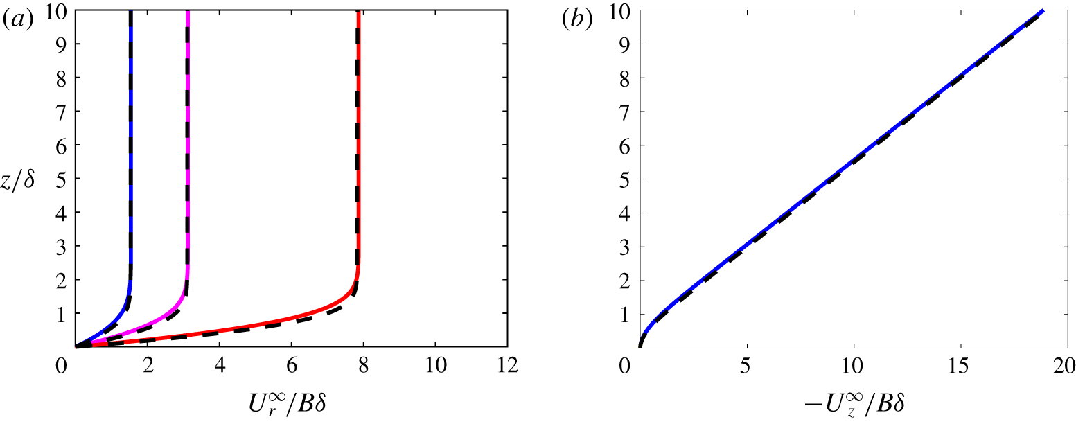
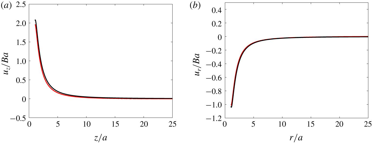
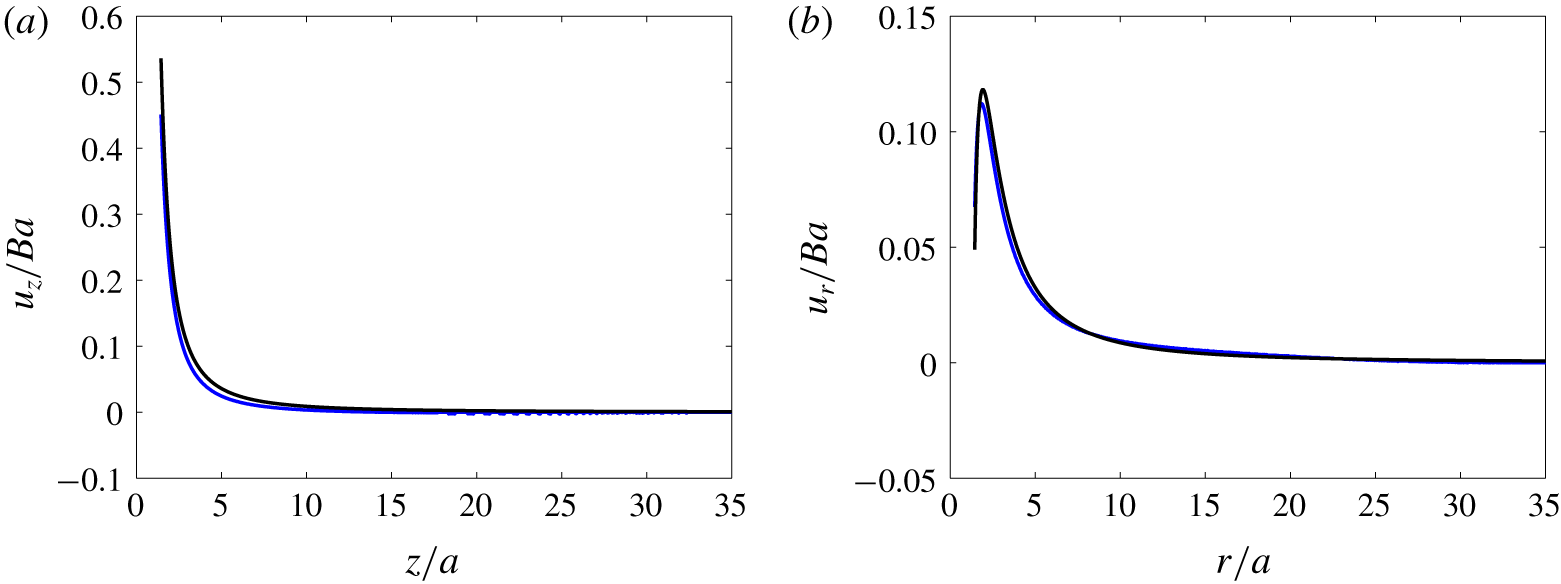
Comparison between computational predictions (dashed lines) and the theoretical HH solution (solid coloured lines) for the undisturbed fluid velocity distribution. (a) Radial velocity profiles at various radial positions, namely  $r/\unicode[STIX]{x1D6FF}=1.54$ (blue), 3.12 (magenta) and 7.86 (red); (b) wall-normal velocity profile at
 $r/\unicode[STIX]{x1D6FF}=1.54$. The grid is identical to that used in cases
 $c_{1}{-}d_{0}$ defined in table 1.

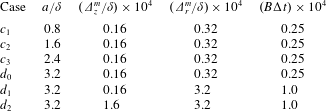
Parameters used in the simulations. Second column: particle radius scaled by  $\unicode[STIX]{x1D6FF}$; third and fourth columns: normalized minimum grid size in the axial and radial directions, respectively; fifth column: normalized time step.

As figure 2 shows, the computed radial and wall-normal components of the velocity field at steady state are in good agreement with the theoretical solution. The corresponding computation makes use of a non-uniform grid distribution; the minimum grid size (near the stagnation point) in both directions is reported in table 1 (case  $c_{1}$). A set of several tests allowed us to conclude that simulation achieves grid independence with respect to the single-phase flow as soon as the minimum cell size in the wall-normal direction,
 $\unicode[STIX]{x1D6E5}_{z}^{m}$, is below
 $0.08\unicode[STIX]{x1D6FF}$. The boundary condition imposed on the peripheral surface is found to have a negligible effect. The flow incident to the wall must decelerate to satisfy the no-penetration condition. This deceleration leads to a volume force directed away from the wall. Before examining the particle dynamics, let us consider the force
 $\boldsymbol{F}^{\infty }$ that would be experienced by a fluid element with the same finite volume as the rigid particle, namely
 ${\mathcal{V}}_{p}={\textstyle \frac{4}{3}}\unicode[STIX]{x03C0}a^{3}$. This force is merely (Maxey & Riley Reference Maxey and Riley1983; Auton, Hunt & Prud’Homme Reference Auton, Hunt and Prud’Homme1988)
 $$\begin{eqnarray}\boldsymbol{F}^{\infty }=\int _{{\mathcal{V}}_{p}}\unicode[STIX]{x1D70C}\frac{\text{D}\boldsymbol{U}^{\infty }}{\text{D}t}\,\text{d}{\mathcal{V}},\end{eqnarray}$$
where  $\text{D}/\text{D}t$ denotes the material derivative along the path of the fluid element and
 $\boldsymbol{U}^{\infty }$ refers to the undisturbed fluid velocity. Equation (3.1) indicates that a finite-size rigid body transported by the HH flow is subject to an inertial force, irrespective of the disturbance it introduces in the flow. Away from the boundary layer, the flow is virtually inviscid and the fluid deceleration is just balanced by the pressure increase toward the stagnation point. In that region, the strain is uniform and the velocity distribution varies linearly with the current position. Consequently, the ambient force defined in (3.1) tends to
 $\boldsymbol{F}^{\infty }=\unicode[STIX]{x1D70C}{\mathcal{V}}_{p}(\text{D}\boldsymbol{U}^{\infty }/\text{D}t)|_{\boldsymbol{x}=\boldsymbol{x}_{c}}$, where
 $\boldsymbol{x}_{c}$ denotes the position of the sphere centre.
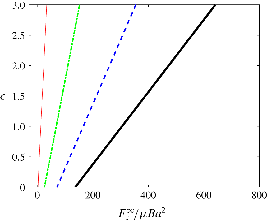
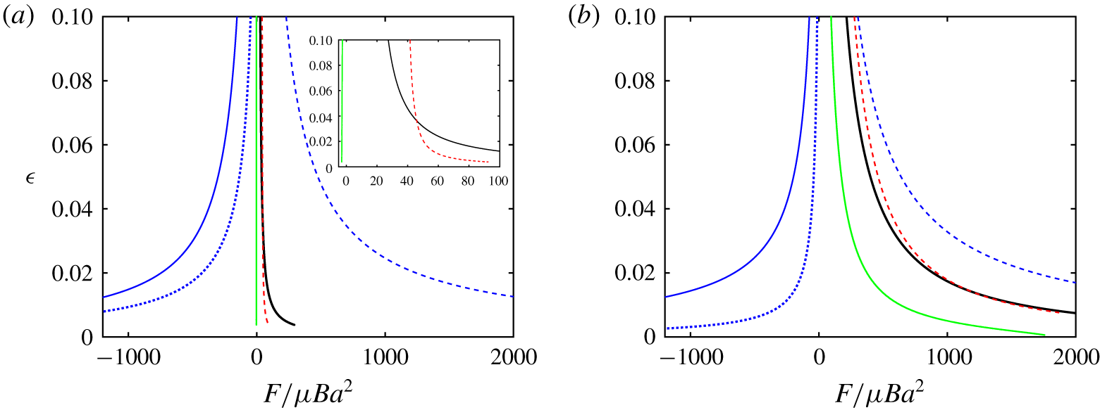
Figure 3 shows the axial profiles of the wall-normal component  $F_{z}^{\infty }$ of
 $\boldsymbol{F}^{\infty }$ computed according to (3.1) for four fictitious fluid spheres with increasing size. Since the ambient force scales as the sphere volume,
 $F_{z}^{\infty }$ increases with the sphere size once normalized by the viscous force scale
 $\unicode[STIX]{x1D707}Ba^{2}$. The force also increases with the axial sphere position
 $z_{c}$ with respect to the wall, hence with the dimensionless gap
 $\unicode[STIX]{x1D716}=h/a=z_{c}/a-1$. This is a direct consequence of the increase of the fluid acceleration,
 $(\boldsymbol{U}^{\infty }\boldsymbol{\cdot }\unicode[STIX]{x1D735})\boldsymbol{U}^{\infty }$, with
 $z_{c}$. When
 $\unicode[STIX]{x1D716}=0$ (i.e. the sphere touches the wall), the fluid acceleration at the position
 $z_{c}=a$ of the sphere centre remains non-zero because
 $a$ is finite. This is why, in figure 3,
 $F_{z}^{\infty }$ is observed to be non-zero at the wall, although it clearly goes to zero as
 $a/\unicode[STIX]{x1D6FF}\rightarrow 0$.
Ambient inertial force  $F_{z}^{\infty }$ acting on a fluid sphere with radius
 $a$ standing a distance
 $z_{c}$ from the wall, as a function of the dimensionless gap
 $\unicode[STIX]{x1D716}=h/a$, with
 $h=z_{c}-a$. Red, green, blue and black lines correspond to
 $a/\unicode[STIX]{x1D6FF}=0.8$, 1.6, 2.4 and 3.2, respectively.

4 How neutrally buoyant particles approach the stagnation point
We now consider the dynamics of a solid sphere in the HH flow in the case where the fluid and particle densities are equal. This neutrally buoyant system allows us to explore the role of inertial effects associated specifically with the size of the suspended particle, and disentangle them from the role of the solid-to-fluid inertia ratio,  $\unicode[STIX]{x1D70C}_{p}/\unicode[STIX]{x1D70C}$. The parameters of the computational study are presented in table 1. Once the carrying flow has reached a steady state, a rigid particle is released from rest with its centre of mass standing on the symmetry axis, far outside the boundary layer, and away from the outer boundary of the simulation domain. The initial particle position was arbitrarily set at
 $z_{p0}=16\unicode[STIX]{x1D6FF}$ in most of the simulations, a position at which the local fluid velocity is approximately
 $-2Bz_{p0}$. After being released from rest, the particle quickly reaches the local fluid velocity, so that the relative velocity between the particle and fluid takes negligibly small values well before the particle starts to interact with the boundary layer. We varied the initial position (
 $12\leqslant z_{p0}/\unicode[STIX]{x1D6FF}\leqslant 20$) in order to verify that it has no influence on the near-wall dynamics. We consider particles with sizes
 $a/\unicode[STIX]{x1D6FF}=0.8$, 1.6, 2.4 and 3.2, so that the Reynolds number
 $Re=2Ba^{2}/\unicode[STIX]{x1D708}=2(a/\unicode[STIX]{x1D6FF})^{2}$ ranges approximately from 1 to 20. The computational grid is non-uniform, being highly refined near the stagnation point to capture lubrication effects without resorting to a model. The minimum size of the near-stagnation-point grid cells in both directions is indicated in table 1. With the largest particle, a typical grid comprises
 $3.6\times 10^{5}$ cells approximately, and
 $1.2\times 10^{4}$ time steps are required to track the particle from its initial position down to very small gaps. Each computation run on a single node equipped with 20 cores of the Olympe supercomputer of the CALMIP computing centre (see
https://www.calmip.univ-toulouse.fr/spip.php?rubrique93) lasts for approximately 2.5 h.
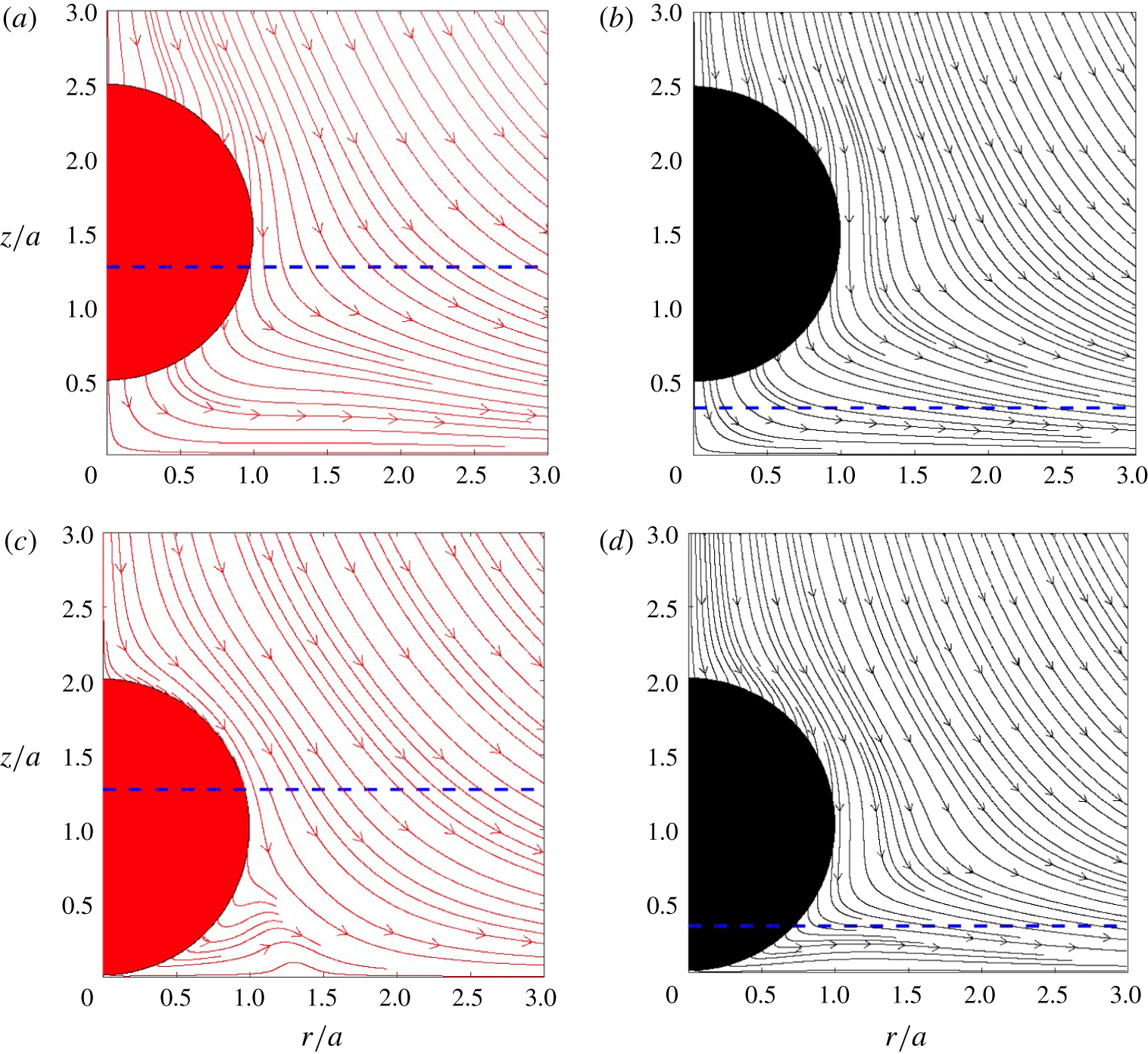
Flow streamlines (in the wall reference frame) about two particles moving toward the wall, at wall-normal positions  $z_{p}/a=1.5$ (a,b) and
 $z_{p}/a=1.01$ (c,d). (a,c) ‘Small’ particle with
 $a/\unicode[STIX]{x1D6FF}=0.8$; (b,d) ‘large’ particle with
 $a/\unicode[STIX]{x1D6FF}=3.2$. The dashed line indicates the distance
 $z/a=\unicode[STIX]{x1D6FF}/a$ from the wall.

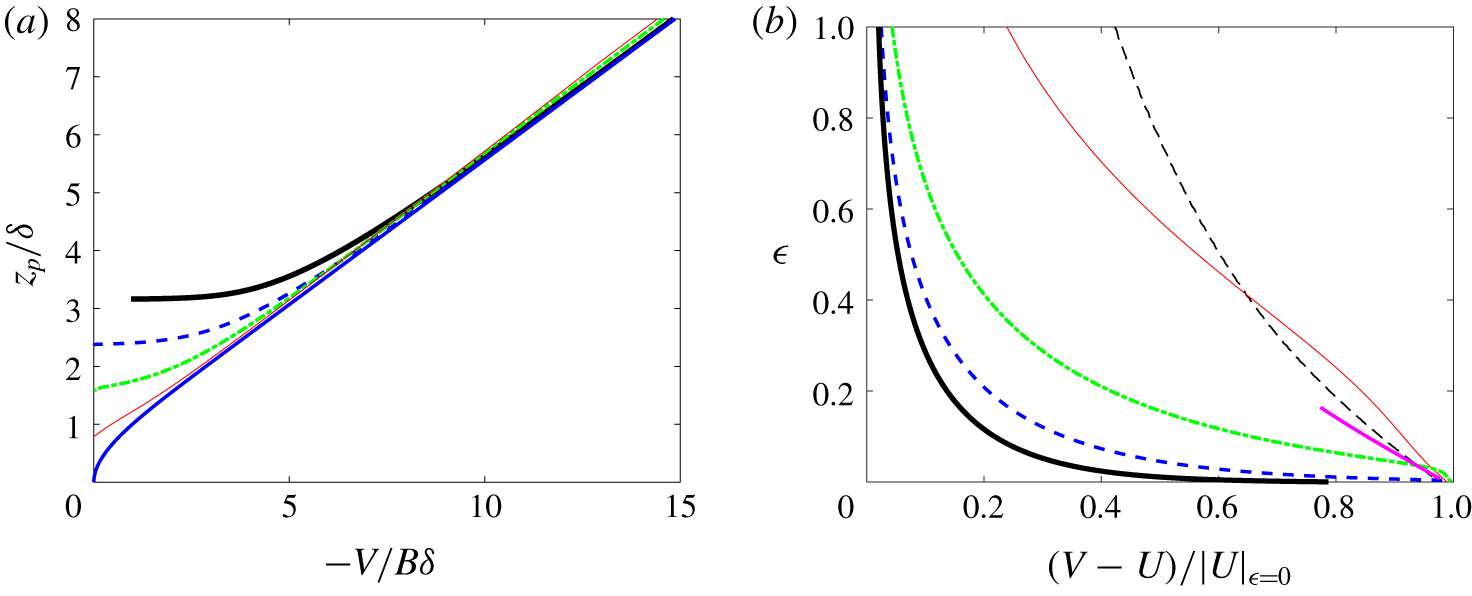
Particle velocity and particle–fluid slip velocity as a function of the distance to the wall. (a) Particle velocity versus the normalized wall-normal position of the particle centre  $z_{p}/\unicode[STIX]{x1D6FF}$; (b) slip velocity scaled by the fluid velocity at
 $z=a$ (
 $\unicode[STIX]{x1D716}=0$), as a function of the dimensionless gap.
 $a/\unicode[STIX]{x1D6FF}=3.2$ (black line), 2.4 (dotted blue line), 1.6 (dash-dotted green line), 0.8 (red line); blue solid line in (a): tracer-like particle; black dashed line in (b):
 $a/\unicode[STIX]{x1D6FF}=0.1$. The pink line in (b) corresponds to the theoretical prediction for the slip in the Stokes flow limit obtained with
 $a/\unicode[STIX]{x1D6FF}=0.01$ and
 $\unicode[STIX]{x1D716}\rightarrow 0$ (Rallabandi et al. Reference Rallabandi, Hilgenfeldt and Stone2017).

4.1 Flow disturbance, slip velocity and hydrodynamic force
The flow field about the smallest and largest particles considered throughout §§ 4 and 5 is displayed in figure 4 at two near-wall positions corresponding to dimensionless gaps  $\unicode[STIX]{x1D716}=0.5$ and
 $\unicode[STIX]{x1D716}=0.01$. Keeping in mind that the outer edge of the boundary layer is located at the wall-normal position
 $z\approx 3\unicode[STIX]{x1D6FF}$, the small particle is seen to be already totally immersed within the boundary layer when
 $\unicode[STIX]{x1D716}=0.5$. In contrast, only the lower one fourth of the large particle stands within the boundary layer at the same
 $\unicode[STIX]{x1D716}$, and this fraction has only increased to one half by the time the dimensionless gap has decreased to 0.01. Consequently, one may expect the two particles to experience quite different near-wall dynamics. This is confirmed by comparing the two streamline patterns for
 $\unicode[STIX]{x1D716}=0.01$. As these streamlines are based on the absolute velocity with respect to the wall, the local angle they make with the particle surface gives insight into the ratio of the radial and tangential components of the relative fluid velocity with respect to the particle. Considering the upper half of each particle, this angle is seen to be large in both cases when
 $\unicode[STIX]{x1D716}=0.5$. In contrast, streamlines have become almost parallel to the upper half of the surface of the small particle when the gap has reduced to 0.01, while they keep a significant angle with the surface in the case of the large particle. This is a clear indication that the small particle has virtually been brought to rest in between the two positions, while the velocity of the large particle is still significant when it gets very close to the wall. On the part of the particle nearest to the wall, the angle made by the streamlines with the surface has decreased in between the two positions but is still far from zero for both particles when
 $\unicode[STIX]{x1D716}=0.01$. We emphasize this non-zero angle to call attention to the existence of a substantial radial fluid motion in the thin film filling the gap, a configuration prone to produce large lubrication forces. This radial motion weakens as the distance to the flow axis increases, as underlined by the marked bulge visible in the streamline pattern around the small particle in the range
 $1\lesssim r/a\lesssim 1.5$. This zone marks the transition between the squeezing of the film in the thin wall–particle gap and the undisturbed boundary layer of the HH flow.
Variations of the particle velocity are shown in figure 5 as a function of the wall-normal position  $z_{p}/\unicode[STIX]{x1D6FF}$, for the four particle sizes listed in table 1. The particle velocity is compared with the fluid velocity along the
 $z$-axis. Far from the wall, the particle is carried with negligible relative motion (slip) with respect to the undisturbed flow. However, the slip increases as the distance separating the particle from the wall decreases. Figure 5(b) shows the slip profiles as a function of the dimensionless gap. The slip is scaled by the undisturbed fluid velocity taken a distance
 $z=a$ from the wall, which is approximately equal to
 $-2Ba$ for
 $a=\mathit{O}(\unicode[STIX]{x1D6FF})$. This scaling limits slip variations between 0, when the particle is not affected by the wall, and 1, when it touches it, so that all curves in figure 5(b) converge to 1 as
 $\unicode[STIX]{x1D716}\rightarrow 0$. This figure indicates that the separation distance (scaled by
 $a$) at which the slip starts to depart from zero decreases with the particle size (compare the slip at
 $\unicode[STIX]{x1D716}=1$ for the smallest two particles with that corresponding to the other three). For large particles, the slip velocity remains negligible down to small gaps. Then it increases abruptly after the gap decreases to a fraction of the particle radius.
Some theoretical insight may be obtained into the way the slip velocity varies with respect to the gap in the creeping-flow limit, which here corresponds to the limit of small particles such that  $a/\unicode[STIX]{x1D6FF}\ll 1$. Using bipolar coordinates, Rallabandi et al. (Reference Rallabandi, Hilgenfeldt and Stone2017) computed the various contributions to the hydrodynamic force involved in the approach of a rigid sphere to a wall in the case the sphere is immersed in a non-uniform quadratic axisymmetric flow. For the HH flow considered here, their results show that the force balance reduces to
 $$\begin{eqnarray}\underbrace{-6\unicode[STIX]{x03C0}\unicode[STIX]{x1D707}a^{2}{\mathcal{B}}(\unicode[STIX]{x1D716})\unicode[STIX]{x1D735}_{z}U}_{F_{{\mathcal{B}}}}+\underbrace{6\unicode[STIX]{x03C0}\unicode[STIX]{x1D707}a^{3}{\mathcal{C}}(\unicode[STIX]{x1D716})\unicode[STIX]{x1D735}_{z}\unicode[STIX]{x1D735}_{z}U}_{F_{{\mathcal{C}}}}+\underbrace{6\unicode[STIX]{x03C0}\unicode[STIX]{x1D707}a{\mathcal{A}}(\unicode[STIX]{x1D716})(U-V)}_{F_{{\mathcal{A}}}}\approx 0,\end{eqnarray}$$
where  $\unicode[STIX]{x1D735}_{z}=\boldsymbol{e}_{\boldsymbol{z}}\boldsymbol{\cdot }\unicode[STIX]{x1D735}$ is the wall-normal gradient (with
 $\boldsymbol{e}_{\boldsymbol{z}}$ the unit vector pointing in the direction of increasing
 $z$),
 $U\equiv U_{z}^{\infty }=\boldsymbol{U}^{\infty }\boldsymbol{\cdot }\boldsymbol{e}_{\boldsymbol{z}}$,
 $V\equiv \boldsymbol{V}\boldsymbol{\cdot }\boldsymbol{e}_{\boldsymbol{z}}$ and
 ${\mathcal{A}}(\unicode[STIX]{x1D716})$,
 ${\mathcal{B}}(\unicode[STIX]{x1D716})$ and
 ${\mathcal{C}}(\unicode[STIX]{x1D716})$ are dimensionless positive gap-dependent coefficients. In the limit of large gaps,
 ${\mathcal{A}}(\unicode[STIX]{x1D716})\rightarrow 1$,
 ${\mathcal{B}}(\unicode[STIX]{x1D716})\rightarrow {\textstyle \frac{15}{16}}\unicode[STIX]{x1D716}^{-2}$ and
 ${\mathcal{C}}(\unicode[STIX]{x1D716})\rightarrow 1/6$, while all three coefficients diverge as
 $1/\unicode[STIX]{x1D716}$ when the gap tends to zero. The force
 $F_{{\mathcal{A}}}$ is just the drag force the particle would experience, were it settling toward the wall in a uniform flow. As discussed by Magnaudet & Abbas (Reference Magnaudet and Abbas2020), the force
 $F_{{\mathcal{B}}}$ results from the interaction of the sphere-induced disturbance, dominated by a stresslet (the first contribution on the right-hand side of (A 1)), with the wall. This interaction generates a flow correction directed away from the wall, therefore tending to repel the particle from the wall, hence enhancing the slip velocity
 $V-U$. Within the boundary layer, the wall-normal velocity
 $U$ becomes gradually a quadratic function of
 $z$ as
 $z\rightarrow 0$. Therefore, in addition to the aforementioned stresslet, the sphere-induced disturbance also contains a Stokes quadrupole, the magnitude of which increases as the gap goes to zero. The force
 $F_{{\mathcal{C}}}$ combines the familiar Faxén force resulting from the non-zero curvature of
 $U$, with a specific wall-induced effect resulting from the interaction of this quadrupole with the wall. As the curvature
 $\unicode[STIX]{x2202}_{z}^{2}U$ is negative, the force proportional to
 ${\mathcal{C}}$ tends to drive the particle toward the wall. The slip velocity predicted by (4.1) is plotted in figure 5(b) (pink line) in the limit
 $\unicode[STIX]{x1D716}\ll 1$. Note that the solution in the Stokes limit depends on the particle size with respect to the flow macro-scale, i.e.
 $\unicode[STIX]{x1D6FF}$ in the present configuration. The pink line was obtained using
 $a/\unicode[STIX]{x1D6FF}=0.01$. The slip velocity of a small particle with
 $a/\unicode[STIX]{x1D6FF}=0.1$ is also displayed in that figure, as it represents an intermediate case between the Stokes limit and particles with
 $a=\mathit{O}(\unicode[STIX]{x1D6FF})$. Clearly, there is a non-monotonic change in the profiles of the slip velocity when the particle size increases. In the Stokes limit as well as for the small particle with
 $a/\unicode[STIX]{x1D6FF}=0.1$, the slip increases monotonically while the particle approaches the wall. As the particle size becomes of the order of
 $\unicode[STIX]{x1D6FF}$, the profile undergoes a qualitative shape change. Indeed, profiles corresponding to
 $a/\unicode[STIX]{x1D6FF}=0.8$ and 1.6 exhibit an inflexion point. The larger the particle, the closer to the wall the position of the inflexion point. We shall come back to this feature later. No inflexion point is observed on the profiles corresponding to the largest two particles with
 $a/\unicode[STIX]{x1D6FF}=2.4$ and 3.2, for which the slip departs significantly from zero only in the late stage of the approach toward the wall.
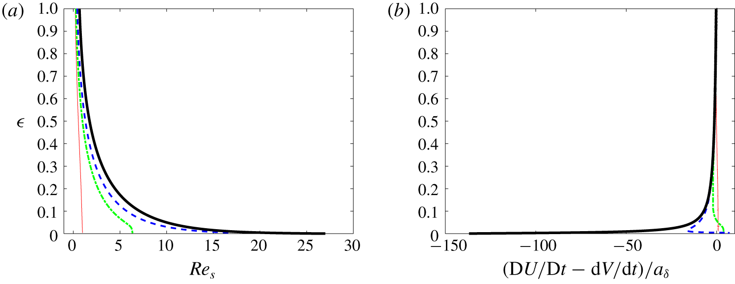
Two characteristics of the differential motion between the particle and fluid for different particle sizes: (a) slip Reynolds number,  $Re_{s}$; (b) relative acceleration,
 $(\text{D}U/\text{D}t)-(\text{d}V/\text{d}t)$, normalized by
 $a_{\unicode[STIX]{x1D6FF}}=\unicode[STIX]{x1D6FF}B^{2}$.
 $a/\unicode[STIX]{x1D6FF}=3.2$ (black line), 2.4 (dotted blue line), 1.6 (dash-dotted green line), 0.8 (red line).

Figure 6(a) shows how the slip Reynolds number,  $Re_{s}=2a(V-U)/\unicode[STIX]{x1D708}$, varies with the distance to the wall. Starting from negligible values for large separations,
 $Re_{s}$ grows as the wall is approached. While this increase remains moderate down to the wall when
 $a/\unicode[STIX]{x1D6FF}<1$, it becomes dramatic for larger particles when
 $\unicode[STIX]{x1D716}\rightarrow 0$. In particular,
 $Re_{s}$ reaches wall values in the range
 $[15,30]$ for the largest two particles. Similarly, the differential acceleration between the fluid and the particle grows sharply while the wall is approached, as seen in figure 6(b). Since the slip goes from near-zero values when the gap is large to a finite positive value when
 $\unicode[STIX]{x1D716}=0$, the differential acceleration
 $\text{D}U/\text{D}t-\text{d}V/\text{d}t$ is generally negative throughout the near-wall region. Nevertheless it may change its sign near the wall, as seen for
 $a/\unicode[STIX]{x1D6FF}=1.6$ and 2.4. We shall come back to this point later. Large particles reach the wall while their centre is still outside the boundary layer. Therefore, in the neighbourhood of the upper part of the particle surface, the fluid is slowed down (due to the no-slip condition) at positions where it is not yet undergoing viscous slowing due to boundary-layer effects. As a consequence the magnitude of the differential acceleration dramatically increases with the particle size in the immediate wall vicinity.
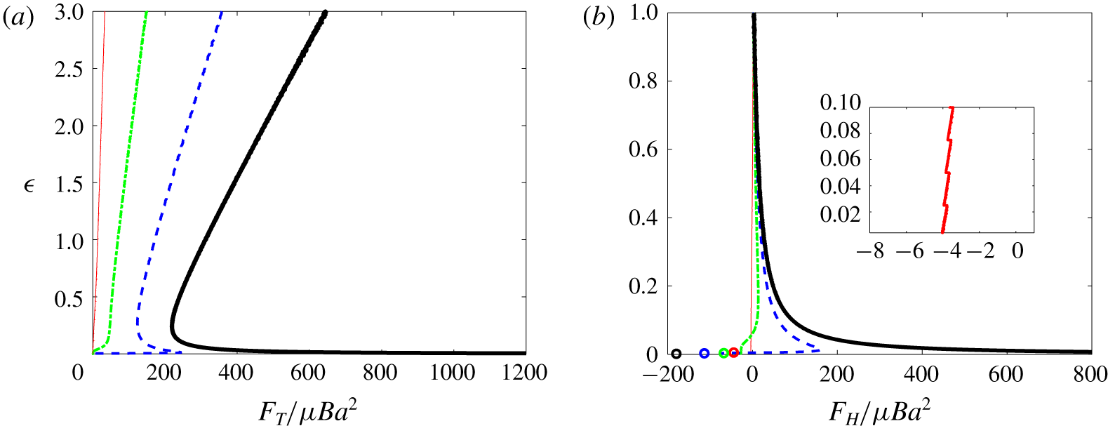
Figure 7(a) displays the profiles of the total force  $F_{T}$ exerted by the fluid on the particle, defined as the
 $z$-projection of the right-hand side of (2.3). Profiles of the difference
 $F_{H}=F_{T}-F_{z}^{\infty }$ between the total and ambient forces are shown in figure 7(b) for
 $\unicode[STIX]{x1D716}\leqslant 1$. In what follows, the force difference
 $F_{H}$ is termed the ‘hydrodynamic’ force, as it results entirely from the disturbance induced by the presence of the particle. By the way it is defined,
 $F_{H}$ is proportional to the difference between the particle and fluid accelerations, as the comparison with figure 6(b) confirms. Although it is the most obvious indicator that can be extracted from the simulations to characterize the particle dynamics, the force
 $F_{H}$ provides limited insight into the physical mechanisms involved. The reason for this is that
 $F_{H}$ represents the sum of all hydrodynamic forces acting on the particle, with the exception of the ambient force
 $F_{z}^{\infty }$. For instance, suppose the particle is small enough for the creeping-flow analysis of Rallabandi et al. (Reference Rallabandi, Hilgenfeldt and Stone2017) to be applicable. Then, inertial effects such as the force associated with the particle inertia,
 $\unicode[STIX]{x1D70C}_{p}{\mathcal{V}}_{p}\,\text{d}V/\text{d}t$ (with here
 $\unicode[STIX]{x1D70C}_{p}=\unicode[STIX]{x1D70C}$), or the ambient force,
 $F_{z}^{\infty }$, are negligibly small compared to zero-Reynolds-number effects such as the viscous drag. As
 $F_{H}$ is merely the difference between these two inertial forces, it is also negligibly small, as figure 7(b) confirms in the case of the smallest particle (
 $a/\unicode[STIX]{x1D6FF}=0.8$). However,
 $F_{H}$ may alternatively be written as the sum of all viscous forces involved in (4.1), i.e.
 $F_{H}=F_{{\mathcal{A}}}+F_{{\mathcal{B}}}+F_{{\mathcal{C}}}$. Although each of these forces is large in magnitude, their sum is small, and thus
 $F_{H}$ provides no insight into the magnitude of individual viscous effects.
Variation of the forces experienced by the particle with respect to the wall-normal position. (a) Total force,  $F_{T}$; (b) hydrodynamic force,
 $F_{H}=F_{T}-F_{z}^{\infty }$. In (b), symbols indicate the value taken by
 $F_{H}$ when the particle is held fixed at the stagnation point (the colour code is identical to that used for the force profiles). The inset shows the variations of
 $F_{H}$ for the particle corresponding to
 $a/\unicode[STIX]{x1D6FF}=0.8$ very close to the wall. The line style refers to the particle size:
 $a/\unicode[STIX]{x1D6FF}=3.2$ (black line), 2.4 (dotted blue line), 1.6 (dash-dotted green line), 0.8 (red line).

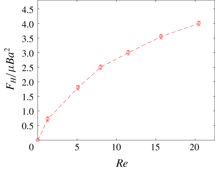
Variation of the ‘hydrodynamic’ force  $F_{H}$ with the particle Reynolds number at the location corresponding to
 $\unicode[STIX]{x1D716}=1$ for each particle in the range
 $0.1\leqslant a/\unicode[STIX]{x1D6FF}\leqslant 3.2$. Error bars correspond to the maximum deviation observed when the particle initial position
 $z_{p0}/\unicode[STIX]{x1D6FF}$ is varied from 12 to 20.

At the present stage, the only expectation with respect to  $F_{H}$ is that, given its nature, it should be an increasing function of the Reynolds number at a given
 $\unicode[STIX]{x1D716}$. This is confirmed by figure 8 in which
 $F_{H}$ is plotted against
 $Re=2Ba^{2}/\unicode[STIX]{x1D708}$ at the location corresponding to
 $\unicode[STIX]{x1D716}=1$ for particles corresponding to
 $a/\unicode[STIX]{x1D6FF}\geqslant 0.1$. Once normalized using the viscous scaling
 $\unicode[STIX]{x1D707}Ba^{2}$,
 $F_{H}$ is seen to increase gradually from a negligibly small value to approximately 4 while
 $Re$ goes from ≈0.02 for the smallest particle to ≈20.5 for the largest one. In this figure, we have gathered results obtained using various release positions of the particle,
 $12\leqslant z_{p0}/\unicode[STIX]{x1D6FF}\leqslant 20$. Considering the small variations of the hydrodynamic force recorded at
 $\unicode[STIX]{x1D716}=1$, it may be concluded that present computational predictions in the near-wall region are insensitive to the choice of
 $z_{p0}$ and are therefore representative of a particle approaching the wall from infinity.
Let us now focus on the dynamics of the particle very close to the wall ( $\unicode[STIX]{x1D716}\ll 1$). First of all, it is important to note that
 $F_{T}$ must eventually vanish when the particle touches the wall. This directly results from the definition of
 $F_{T}$ as the
 $z$-projection of the right-hand side of (2.3) and of the vanishing of the particle acceleration at the wall: since
 $\text{d}V/\text{d}t=V\,\text{d}V/\text{d}z$ and
 $V=0$ when
 $\unicode[STIX]{x1D716}=0$, it follows that
 $F_{T}(\unicode[STIX]{x1D716}=0)=0$. When
 $\unicode[STIX]{x1D716}\ll 1$, the evolution of the particle velocity and that of the hydrodynamic force depend strongly on the particle size, as figures 5–7 revealed. The particle speed decreases below that of a fluid tracer, as shown in figure 5, owing to additional wall-induced forces, especially the one associated with the wall-normal gradient of the carrying flow in (4.1) or its finite-
 $Re$ counterpart. The smaller-size particles (
 $a/\unicode[STIX]{x1D6FF}=0.8$ and 1.6) decelerate drastically and the total force
 $F_{T}$ tends monotonically to zero as seen in figure 7(a). For these particles,
 $F_{H}$ becomes negative (see figure 7b), which means that the (toward wall) drag force exceeds the sum of all wall-induced contributions (to be detailed later).
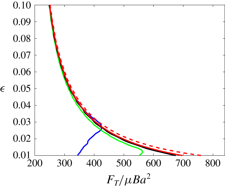
Effect of the near-wall numerical resolution on the total force  $F_{T}$ acting on the largest particle (
 $a/\unicode[STIX]{x1D6FF}=3.2$) at small gaps. The line style refers to the grid in table 1:
 $d_{2}$ (black),
 $d_{1}$ (red solid),
 $d_{0}$ (red dashed). Additional under-resolved runs with a minimum cell size
 $\unicode[STIX]{x1D6E5}_{z}^{m}/\unicode[STIX]{x1D6FF}=0.08$ (blue) and 0.04 (green), both with
 $B\unicode[STIX]{x0394}t=1\times 10^{-4}$.

As seen in figure 5, the rate of approach to the wall of larger particles ( $a/\unicode[STIX]{x1D6FF}=2.4$ and 3.2) remains considerably larger for small gaps. As a consequence, the magnitude of the total force does not decrease monotonically. Instead,
 $F_{T}$ decreases on approach only until
 $\unicode[STIX]{x1D716}\approx 0.2$. Then the resistive force due to lubrication grows and becomes dominant, yielding a strong particle deceleration, i.e. a large positive
 $\text{d}V/\text{d}t$ since
 $V<0$. For
 $a/\unicode[STIX]{x1D6FF}=2.4$, the lubrication force is able to bring the particle virtually to rest, so that
 $\text{d}V/\text{d}t$ becomes small and
 $F_{T}$ eventually tends to zero. Since the fluid decelerates down to the wall,
 $F_{z}^{\infty }$ remains positive down to
 $\unicode[STIX]{x1D716}=0$ (i.e. it pushes the particle away from the wall), so that
 $F_{H}=F_{T}-F_{z}^{\infty }$ eventually becomes negative. As figure 7(b) shows, the latter trend is actually observed whatever the particle size. For the largest particle (
 $a/\unicode[STIX]{x1D6FF}=3.2$),
 $F_{T}$ is still dramatically rising at
 $\unicode[STIX]{x1D716}=0.01$, the minimum value allowed by the computational grid. A zoom of its behaviour very close to the wall is provided in figure 9. This zoom emphasizes how refined the grid resolution has to be close to the wall for the force divergence to be correctly captured at gaps less than a few per cent of the particle radius. As may be expected, the curves obtained with a purposely under-refined grid (blue and green lines in figure 9) exhibit a ‘kink’ when
 $\unicode[STIX]{x1D716}\rightarrow 0$, due to under-resolution. This is totally distinct from the local maximum exhibited in figure 7(a) by
 $F_{T}$ for
 $a/\unicode[STIX]{x1D6FF}=2.4$ which has a real physical basis as discussed above. With the grid parameters used here, it is clear that we do not resolve the flow sufficiently well to capture the return to zero of
 $F_{T}$ for
 $a/\unicode[STIX]{x1D6FF}=3.2$. However, theory predicts that lubrication eventually decelerates the particle whatever its size, so that
 $F_{T}$ should also reach a local maximum in that case. Considering the last stage of approach observed with
 $a/\unicode[STIX]{x1D6FF}=2.4$, we may infer that
 $F_{H}$ also decreases and becomes eventually negative with
 $a/\unicode[STIX]{x1D6FF}=3.2$, although our computations do not capture this stage.
A primary finding obtained from the simulations analysed above is that the total force acting on a decelerating neutrally buoyant particle approaching a stagnation point at a wall exhibits a transition according to its size. For  $a/\unicode[STIX]{x1D6FF}\lesssim 1.6$, the total force experienced by the particle decreases monotonically to zero, while for
 $a/\unicode[STIX]{x1D6FF}\gtrsim 2.4$ it increases sharply near the wall, before returning to zero. In the former case, long-range hydrodynamic effects, such as the repelling wall-induced force in (4.1), are capable of efficiently slowing down the particle before lubrication effects come into play. In contrast, inertial effects associated with the disturbance flow for large enough particles make them able to keep a significant speed down to separations where part of their surface is already very close to the wall. Their abrupt deceleration imposed by lubrication effects is responsible for the non-monotonic evolution of the total force at very small gaps. This change of behaviour has a significant practical importance: if the gap between the particle and the wall becomes comparable to the characteristic surface roughness of the wall or particle while the particle velocity is still finite, the continuum description breaks down and solid contact is expected to occur.
4.2 Stress distribution at the particle surface
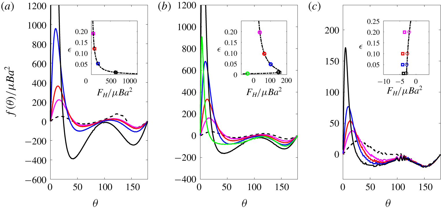
Angular distribution of the contribution  $f(\unicode[STIX]{x1D703})$ to the hydrodynamic force at various gaps and for three particle sizes;
 $\unicode[STIX]{x1D703}$ is in degrees from the position of closest approach to the wall. (a)
 $a/\unicode[STIX]{x1D6FF}=3.2$, (b) 2.4 and (c) 0.8, with
 $\unicode[STIX]{x1D716}=0.005$ (green), 0.01 (black), 0.05 (blue), 0.10 (red) and 0.20 (magenta). Inset:
 $F_{H}$ computed from the right-hand side of (2.3) (circles) or defined as
 $F_{H}=\int _{0}^{\unicode[STIX]{x03C0}}f(\unicode[STIX]{x1D703})\,\text{d}\unicode[STIX]{x1D703}$ (squares).

We now examine several features of the local stress distribution at the particle surface when the gap is small, using the interpolation technique outlined in § 2.
First, defining  $\unicode[STIX]{x1D72E}^{\infty }$ as the stress tensor associated with the undisturbed flow, we compute the disturbance traction
 $\boldsymbol{t}=(\unicode[STIX]{x1D72E}-\unicode[STIX]{x1D72E}^{\infty })\boldsymbol{\cdot }\boldsymbol{n}$ at the particle surface as a function of the angular position
 $\unicode[STIX]{x1D703}$ with respect to its ‘lower’ pole (the point closest to the wall, see figure 1). This allows us to obtain the quantity
 $f(\unicode[STIX]{x1D703})=2\unicode[STIX]{x03C0}a^{2}\sin \unicode[STIX]{x1D703}\boldsymbol{e}_{\boldsymbol{z}}\boldsymbol{\cdot }\boldsymbol{t}$ which is nothing but the local contribution to the overall hydrodynamic force, since
 $\int _{0}^{\unicode[STIX]{x03C0}}f(\unicode[STIX]{x1D703})\,\text{d}\unicode[STIX]{x1D703}=F_{H}$. Profiles of
 $f(\unicode[STIX]{x1D703})$ are shown in figure 10 at several gap values and for three different particle sizes. As the insets in this figure show, values of
 $F_{H}$ obtained by integrating
 $f(\unicode[STIX]{x1D703})$ over the particle surface agree well with those found directly by subtracting
 $F_{z}^{\infty }$ from the right-hand side of (2.3). Nevertheless, differences occur for the smallest particle (figure 10c), an indication that the stress distribution about that small particle is only marginally resolved by the selected discretization (see table 1). The spurious oscillations discernible in some regions of the corresponding angular distributions corroborate this point.
Before commenting on the profiles in figure 10, it is worth pointing out that the characteristics of the small particle ( $a/\unicode[STIX]{x1D6FF}=0.8$) are distinctly different from those of the larger two particles. Indeed, the Reynolds number of the former is of
 $\mathit{O}(1)$ and this particle is entirely immersed within the boundary layer of the HH flow throughout the range of gaps considered here. For instance, for
 $\unicode[STIX]{x1D716}=0.2$, its top pole stands a distance
 $1.76\unicode[STIX]{x1D6FF}$ from the wall, whereas the outer edge of the boundary layer, where the radial component of
 $\boldsymbol{U}^{\infty }$ reaches 98 % of its free-stream value, stands a distance
 $3\unicode[STIX]{x1D6FF}$ (see figure 1). In contrast, the other two particles have Reynolds numbers in the range
 $[10,20]$, and their top pole stands well beyond the outer edge of the boundary layer. In particular, more than half of the largest particle surface is still outside the boundary layer when
 $\unicode[STIX]{x1D716}=0$.
Although the splitting between pressure and viscous stress contributions is not shown in the figure, examination of the two separate contributions reveals that the former is by far the dominant contributor to  $F_{H}$. Only for the smallest particle is the viscous stress significant far from the poles, say for
 $45^{\circ }\leqslant \unicode[STIX]{x1D703}\leqslant 135^{\circ }$. When the gap decreases to
 $\unicode[STIX]{x1D716}=0.1$,
 $f(\unicode[STIX]{x1D703})$ rises in the region closest to the wall for the largest two particles, say for
 $\unicode[STIX]{x1D703}\lesssim 30^{\circ }$, whereas it remains almost unchanged on the rest of their surface. For the smallest particle,
 $f(\unicode[STIX]{x1D703})$ also rises in the region
 $\unicode[STIX]{x1D703}\lesssim 20^{\circ }$, but it decreases on the rest of the half of the surface closest to the wall. For all three particles, the rise of
 $f(\unicode[STIX]{x1D703})$ on this leading part goes on as the gap further decreases. However, changes in the distribution also start to affect the rest of the surface for the largest two, and become prominent for
 $\unicode[STIX]{x1D716}=0.01$. Indeed, for this gap value, the distribution of
 $f(\unicode[STIX]{x1D703})$ exhibits two marked minima respectively located around
 $\unicode[STIX]{x1D703}=45^{\circ }$ and
 $\unicode[STIX]{x1D703}=155^{\circ }$, especially for the largest particle (black line in figure 10a). In the case of the smallest particle, changes in
 $f(\unicode[STIX]{x1D703})$ remain confined to the half of the surface nearest the wall throughout the entire range of gaps. Considering the evolution of the complete pole-to-pole distribution, it appears that the part of the surface on which
 $f(\unicode[STIX]{x1D703})$ is negative increases with time, i.e. as the flow brings the particle closer to the wall, in all cases. As regions with negative
 $f(\unicode[STIX]{x1D703})$ contribute to make
 $F_{H}$ negative, i.e. to drive the particle to the wall, the repulsive contribution only comes from the part of the surface nearest the wall, the extent of which decreases with the gap. More precisely, defining
 $\unicode[STIX]{x1D703}_{c}$ as the smallest angle at which
 $f(\unicode[STIX]{x1D703})$ becomes negative, the evolutions reported in figure 10 indicate that
 $\unicode[STIX]{x1D703}_{c}(\unicode[STIX]{x1D716}=0.2)\approx 50^{\circ }$, while
 $\unicode[STIX]{x1D703}_{c}(\unicode[STIX]{x1D716}=0.01)\approx 20^{\circ }$.
For the largest two particles, combining the above observations with the behaviour of  $F_{H}$ displayed in the insets of panels (a) and (b) of figure 10, one can conclude that, despite the increase in the surface percentage over which
 $f(\unicode[STIX]{x1D703})$ is negative, the much larger positive values of
 $f(\unicode[STIX]{x1D703})$ in the region
 $\unicode[STIX]{x1D703}\lesssim \unicode[STIX]{x1D703}_{c}$ provide the dominant contribution to
 $F_{H}$ until
 $\unicode[STIX]{x1D716}$ becomes very small. The green line in panel
 $(b)$ shows the very last stage of the evolution once the particle has decelerated to a small velocity. Here, the magnitude of the above two minima and that of the much larger maximum near the front pole have decreased dramatically and
 $\unicode[STIX]{x1D703}_{c}$ has fallen to ≈15°. In this configuration, the negative contribution has become dominant, making
 $F_{H}$ negative. In the case of the smallest particle, no such qualitative changes happen. As mentioned above, the rise of
 $f(\unicode[STIX]{x1D703})$ for
 $\unicode[STIX]{x1D703}<\unicode[STIX]{x1D703}_{c}$ is accompanied by the gradual increase of negative values of
 $f(\unicode[STIX]{x1D703})$ in the range
 $\unicode[STIX]{x1D703}_{c}<\unicode[STIX]{x1D703}<90^{\circ }$. This is not unexpected: since the particle Reynolds number is small, positive and negative contributions have to almost balance each other whatever
 $\unicode[STIX]{x1D716}$, as predicted by (4.1). Hence,
 $F_{H}$ keeps a small magnitude throughout the entire gap range considered here. Since the particle deceleration is very small throughout this range, the total force
 $F_{T}$ is almost zero, so that
 $F_{H}=F_{T}-F_{z}^{\infty }$ has to be negative, as confirmed by the inset in figure 10(c). The same is true for the intermediate particle (
 $a/\unicode[STIX]{x1D6FF}=2.4$) in the very last stage of its approach: the green symbol in the inset of panel (b) indicates that
 $F_{H}$ has become negative after the qualitative changes noticed in the
 $f(\unicode[STIX]{x1D703})$ distribution in between
 $\unicode[STIX]{x1D716}=0.01$ and
 $\unicode[STIX]{x1D716}=0.005$ have taken place. This implies that the negative stress applied by the flow over most of the particle surface has become able to balance (and presumably exceed) the positive contribution provided by the lubrication effect on the small portion closest to the wall, corresponding to
 $\unicode[STIX]{x1D703}<\unicode[STIX]{x1D703}_{c}$. The same would occur with the largest particle, had the grid resolution been sufficient to resolve gaps thinner than those reported in figure 10. Nevertheless, the negative values of
 $F_{H}$ reported in the insets of panels (b) and (c) for the smallest gap are smaller than those found in the case the same particle is held fixed at the wall, as shown by the blue and red symbols in figure 7(b), respectively. Thus, in both cases, the flow resistance in the gap has still a residual positive contribution.
As mentioned above, the divergence of the lubrication force as  $\unicode[STIX]{x1D716}\rightarrow 0$ can in principle bring the particle to rest whatever its size. Actually, the particle–wall interaction at very small gaps is not likely to be exclusively hydrodynamic. On the one hand, the viscous force reaches extremely high values, which may lead to particle and wall deformation depending on their respective mechanical properties (Davis, Serayssol & Hinch Reference Davis, Serayssol and Hinch1986). On the other hand, the roughness of the two surfaces may come into play. Since elasto-hydrodynamic interactions are not accounted for by the immersed boundary technique used here and both surfaces are considered perfectly smooth, we stopped the numerical simulations at the smallest gap displayed in figure 10, assuming that standard fluid mechanics does not apply for smaller gaps.
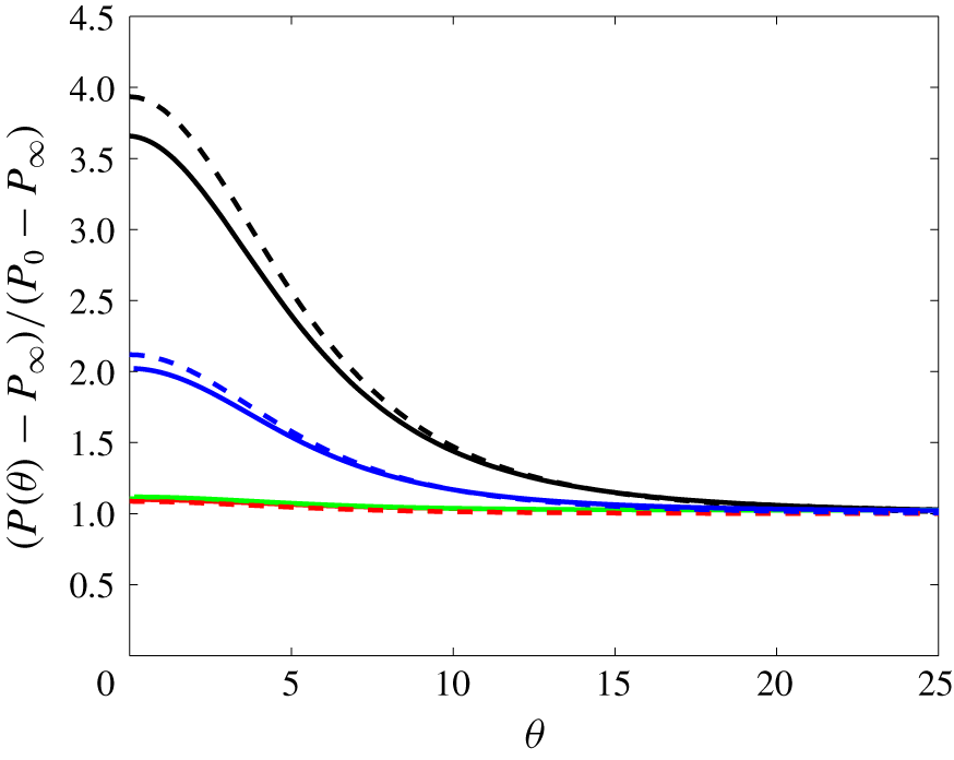
There is no doubt that lubrication effects are responsible for the sharp increase of  $f(\unicode[STIX]{x1D703})$ noticed on the front part of the particle as it approaches the wall. Nevertheless, a quantitative comparison of the corresponding pressure distribution with predictions from lubrication theory is worthwhile. From this theory, it is known that when a rigid body approaches a wall with a finite velocity
 $V$, the viscous resistance grows as
 $1/\unicode[STIX]{x1D716}$ when
 $\unicode[STIX]{x1D716}\ll 1$, yielding a diverging force scaling as
 $\unicode[STIX]{x1D707}a|V|/\unicode[STIX]{x1D716}$ (Cox & Brenner Reference Cox and Brenner1967). This is a consequence of the large pressure required to drive the fluid out of the squeezed film located in the gap. For a rigid sphere approaching a planar wall, the quasi-steady axisymmetric solution for the radial pressure distribution in the creeping-flow regime may be written in the form (Leal Reference Leal2007)
 $$\begin{eqnarray}P(r)-P(R)=6\unicode[STIX]{x1D707}V_{\unicode[STIX]{x1D716}}\int _{R}^{r}\frac{s}{h^{3}(s)}\,\text{d}s.\end{eqnarray}$$
In (4.2),  $h(r)$ is the gap thickness expressed as a function of the radial coordinate
 $r$ (with
 $h(r=0)=\unicode[STIX]{x1D716}a$),
 $V_{\unicode[STIX]{x1D716}}=|V|(z_{p}/a=1+\unicode[STIX]{x1D716})$ is the current sphere speed and
 $R$ is the outermost point of the thin-film region. Since pressure variations across the gap (i.e. in the
 $z$-direction) are assumed to be negligibly small,
 $P(R)$ is almost equal to the pressure
 $P_{0}$ at the stagnation point in the single-phase HH flow. Setting
 $\unicode[STIX]{x1D716}=0.01$ and making use of the particle velocity determined at that position in the simulations, predictions of (4.2) are compared in figure 11 with the previously determined surface pressure distributions. The agreement is good in all cases. The pressure at the point closest to the wall is slightly over-predicted by the lubrication approximation for the largest two particles (by approximately 8 % for
 $a/\unicode[STIX]{x1D6FF}=3.2$), while it is slightly under-predicted for the smallest two.
Pressure profiles along the thin-gap region of the particle surface at  $\unicode[STIX]{x1D716}=0.01$, as a function of the angle in degrees measured from
 $\unicode[STIX]{x1D703}=0$ on the axis of the motion. Solid lines: numerical predictions; dashed lines: thin-gap approximation (4.2), both for
 $a/\unicode[STIX]{x1D6FF}=3.2$ (black), 2.4 (blue), 1.6 (green) and 0.8 (red).

To summarize, we see that the primary findings in terms of the particle dynamics developed in § 4.1 are associated with the controlling influence of the size of the particles, which affects their relation to the boundary-layer thickness. For smaller particles of  $a/\unicode[STIX]{x1D6FF}=0.8$ and 1.6, the hydrodynamic interaction with the wall is able to efficiently reduce the velocity of the particle at sufficient distance to allow a monotonic decrease in the net force on the particle, so that there is an asymptotic approach to the surface in which a drag force due to a lagging slip relative to the carrying flow is balanced by the lubrication flow in the decreasing gap. For the larger particles of
 $a/\unicode[STIX]{x1D6FF}=2.4$ and 3.2, the onset of large slip is delayed until near contact, so that the particle still moves with a velocity near that of the fluid at its centre while part of its surface is very close to the wall, resulting in a very large lubrication force, which grows with the particle size and peaks progressively closer to contact for larger
 $a/\unicode[STIX]{x1D6FF}$. The importance of the boundary-layer flow in determining the detailed form of the stresses has been developed in § 4.2, where the portions of the surface resulting in the drag force toward the surface and the lubrication force are illustrated at several separations.
5 Viscous and inertial effects in the thin-gap limit
In addition to the global hydrodynamic force  $F_{H}$ extracted from the simulations, the material discussed in §§ 4.1 and 4.2 provides two separate ways to estimate the viscous forces at work in the thin-gap limit. First, we may use the force balance (4.1) which is valid down to the wall, provided fluid inertia does not affect the particle-induced disturbance. Second, the leading-order viscous contribution to the force may be obtained through the lubrication approximation, since we just showed that the actual surface pressure distribution in the lubrication gap closely agrees with the corresponding prediction. Assuming that the dimensionless gap
 $\unicode[STIX]{x1D716}$ and gap Reynolds number
 $\unicode[STIX]{x1D716}|Re_{v}|$ are both much smaller than unity, with
 $Re_{v}(\unicode[STIX]{x1D716})=aV(\unicode[STIX]{x1D716})/\unicode[STIX]{x1D708}$, lubrication theory predicts that, in a still fluid, a spherical particle approaching the wall with strictly normal velocity
 $V(\unicode[STIX]{x1D716})$ experiences a wall-normal lubrication force
 ${\mathcal{F}}_{L}(\unicode[STIX]{x1D716})$ such that (Cox & Brenner Reference Cox and Brenner1967)
 $$\begin{eqnarray}{\mathcal{F}}_{L}(\unicode[STIX]{x1D716})=-6\unicode[STIX]{x03C0}\unicode[STIX]{x1D707}a\frac{V(\unicode[STIX]{x1D716})}{\unicode[STIX]{x1D716}}\left[1-\frac{\unicode[STIX]{x1D716}}{5}\left(1-\frac{1}{2}Re_{v}\right)\ln \unicode[STIX]{x1D716}\right].\end{eqnarray}$$
As  $Re_{v}$ is negative (respectively positive) when the particle moves toward (respectively away from) the wall, inertial effects increase the lubrication force in the situation considered here. Using the particle velocity
 $V(\unicode[STIX]{x1D716})$ provided by the simulations, it is straightforward to compute
 ${\mathcal{F}}_{L}(\unicode[STIX]{x1D716})$. Similarly, all forces in (4.1) may be computed using
 $V(\unicode[STIX]{x1D716})$ and the
 $U(z)$-distribution of the undisturbed wall-normal velocity in the vicinity of the particle centre location,
 $z_{p}/a=1+\unicode[STIX]{x1D716}$.
Force profiles in the thin-gap region for (a)  $a/\unicode[STIX]{x1D6FF}=0.8$, and (b)
 $a/\unicode[STIX]{x1D6FF}=3.2$. Hydrodynamic force
 $F_{H}$ (green), lubrication force
 ${\mathcal{F}}_{L}$ (red dashed) and sum
 ${\mathcal{F}}_{0}=F_{{\mathcal{A}}}+F_{{\mathcal{B}}}+F_{{\mathcal{C}}}$ of the three forces involved in the creeping-flow prediction (4.1) (black solid). The blue lines correspond to individual contributions to (4.1):
 $F_{{\mathcal{A}}}$ (solid),
 $F_{{\mathcal{B}}}$ (dashed) and
 $F_{{\mathcal{C}}}$ (dotted). Inset in (a): zoom on the
 $F_{H}$,
 ${\mathcal{F}}_{L}$ and
 ${\mathcal{F}}_{0}$ profiles.

Figure 12 displays the corresponding predictions together with the ‘hydrodynamic’ force  $F_{H}$, for the smallest and largest particles examined in § 4.2 and gaps less than 0.1. In (5.1), the inertial correction is negligibly small (
 ${\leqslant}0.3\,\%$) throughout the considered range of
 $\unicode[STIX]{x1D716}$ for the smallest particle. In contrast, it is significant for the largest one (
 ${\approx}3.2\,\%$ for
 $\unicode[STIX]{x1D716}=0.01$) but the gap Reynolds number is approximately 2.6 when
 $\unicode[STIX]{x1D716}=0.1$, well beyond the limit of validity of the asymptotic theory. For these reasons, the inertial correction is disregarded in the estimate of
 ${\mathcal{F}}_{L}(\unicode[STIX]{x1D716})$ plotted in figure 12. This figure also displays the individual forces involved in (4.1), namely the drag force
 $F_{{\mathcal{A}}}$, and forces
 $F_{{\mathcal{B}}}$ and
 $F_{{\mathcal{C}}}$ resulting from the wall-normal gradient
 $\unicode[STIX]{x2202}_{z}U$ and curvature
 $\unicode[STIX]{x2202}_{z}^{2}U$ of the undisturbed fluid velocity, respectively. In addition to
 $F_{{\mathcal{A}}}$, it is no surprise that
 $F_{{\mathcal{C}}}$ diverges as the wall is approached, since
 $\unicode[STIX]{x2202}_{z}^{2}U$ is non-zero at the wall and the pre-factor
 ${\mathcal{C}}$ in (4.1) is known to diverge as
 $1/\unicode[STIX]{x1D716}$ (Rallabandi et al. Reference Rallabandi, Hilgenfeldt and Stone2017). It is somewhat more subtle to understand why
 $F_{{\mathcal{B}}}$ also diverges as
 $\unicode[STIX]{x1D716}\rightarrow 0$, although the wall-normal velocity gradient
 $\unicode[STIX]{x2202}_{z}U$ vanishes at the wall, owing to the no-slip condition. The reason stands in the finite size of the particle, more specifically in the fact that the particle radius,
 $a$, is not small compared to the characteristic length scale of the flow inhomogeneity,
 $|\unicode[STIX]{x2202}_{z}U|/|\unicode[STIX]{x2202}_{z}^{2}U|$, which is necessarily of
 $\mathit{O}(\unicode[STIX]{x1D6FF})$ in the configuration we consider. For this reason,
 $\unicode[STIX]{x2202}_{z}U$, which depends on
 $a(1+\unicode[STIX]{x1D716})$, tends toward a finite value at the position
 $z_{p}=a$ corresponding to
 $\unicode[STIX]{x1D716}=0$. This is why the velocity gradient, hence
 $F_{{\mathcal{B}}}$, provides another
 $\mathit{O}(\unicode[STIX]{x1D716}^{-1})$ contribution to
 ${\mathcal{F}}_{0}$ in the small-gap limit for particles whose size is of the order of
 $\unicode[STIX]{x1D6FF}$.
Let us now discuss the trends observed in figure 12(a) with the small particle. In line with the discussion in § 4.1, this figure indicates that each of the three forces in (4.1) is much larger than their sum, say  ${\mathcal{F}}_{0}$. The repulsive contribution
 $F_{{\mathcal{B}}}$ is significantly larger than either of the two forces toward the wall, among which is the drag. The resultant force
 ${\mathcal{F}}_{0}$ has the same order of magnitude as
 ${\mathcal{F}}_{L}$, although the inset reveals that the two follow somewhat different evolutions as the gap decreases. The dominant contribution responsible for the
 $\unicode[STIX]{x1D716}^{-1}$-divergence of
 ${\mathcal{F}}_{0}$ as
 $\unicode[STIX]{x1D716}\rightarrow 0$ is provided by the part of the particle surface closest to the wall, which is also by construction the one responsible for the lubrication force, as (4.2) shows. Combined with the fact that
 ${\mathcal{F}}_{0}$ and
 ${\mathcal{F}}_{L}$ were both computed using the actual particle velocity, this remark implies that they necessarily have comparable magnitudes. The lubrication force exceeds
 ${\mathcal{F}}_{0}$ for
 $\unicode[STIX]{x1D716}\gtrsim 0.035$, because it does not include the contribution resulting from the stress on the portion of the particle surface away from the wall, which is negative (i.e. directed toward the wall) as was made clear by figure 10(c). Conversely, the
 $\unicode[STIX]{x1D716}^{-1}$-divergence of
 ${\mathcal{F}}_{L}$ occurs later (i.e. for smaller gaps) than that of
 ${\mathcal{F}}_{0}$. This is because the prediction (5.1) assumes the fluid to be at rest far from the particle, so that possible lubrication-type contributions due to the inhomogeneity of the carrying flow are not directly accounted for. For instance, figure 4(a) revealed the existence of a bulge in the near-wall streamline pattern, in the region where the lubrication film meets the HH flow. This bulge indicates that, compared to the classical situation of a particle settling toward a wall in a fluid at rest, the flow structure within the lubrication film is modified by the outer flow. In the creeping-flow limit, these modifications yield the
 $\mathit{O}(\unicode[STIX]{x1D716}^{-1})$-divergence of forces
 $F_{{\mathcal{B}}}$ and
 $F_{{\mathcal{C}}}$ in (4.1), which in the present case persists down to the wall for the reasons discussed above. Instead, the standard lubrication theory on which (5.1) is grounded only accounts for the
 $\unicode[STIX]{x1D716}^{-1}$-divergence of
 $F_{{\mathcal{A}}}$ in (4.1). Since the repulsive force
 $F_{{\mathcal{B}}}$ is larger than the force
 $F_{{\mathcal{A}}}$ toward the wall for all
 $\unicode[STIX]{x1D716}$, equation (5.1) is expected to under-predict the overall repulsive force experienced by the particle when the gap becomes very small, which is consistent with the behaviour observed in figure 12 for
 $\unicode[STIX]{x1D716}\rightarrow 0$. Note, however, that the particle velocity used in (5.1) is the one provided by the simulation, and this velocity is obviously influenced by the flow inhomogeneities. So (5.1) is actually a mixed approximation in which the lubrication effect is evaluated as if the fluid were at rest at infinity, while the velocity that drives the film squeezing in the gap does take into account the actual properties of the carrying flow.
For reasons similar to those discussed above,  ${\mathcal{F}}_{0}$ and
 ${\mathcal{F}}_{L}$ still exhibit similar profiles and magnitudes throughout the considered gap range in the case of the largest particle (figure 12b). It may also be remarked that the contribution
 $F_{{\mathcal{C}}}$ due to the curvature of the undisturbed flow profile is much smaller than in figure 12(a). The reason is merely that the centre of the large particle considered here stands slightly outside the boundary layer (see figure 4), a position at which the curvature of the
 $U^{\infty }$-profile is still small. In contrast the particle examined in figure 12(a) is fully immersed in the boundary layer, and the parabolic component
 $\unicode[STIX]{x2202}_{z}^{2}U$ of the
 $\boldsymbol{U}^{\infty }$-profile is large at that position.
The difference  ${\mathcal{F}}_{0}-F_{H}$ represents (in absolute value) the sum of all inertial contributions to the force experienced by the particle, apart from the ambient force
 $F_{z}^{\infty }$. This difference is positive for all
 $\unicode[STIX]{x1D716}$ for both particles. According to figures 6 and 8, the slip and shear Reynolds numbers of the small particle in figure 12(a) are both of
 $\mathit{O}(1)$ at such small gaps. Consequently, inertial corrections are expected to alter the zero-
 $Re$ expression of the three forces involved in (4.1), especially that of the drag. The noticeable imbalance between
 ${\mathcal{F}}_{0}$ and
 $F_{H}$ confirms that inertial effects are already significant for Reynolds numbers of
 $\mathit{O}(1)$. In the case of the large particle considered in figure 12(b), the shear Reynolds number is approximately
 $20$ (see figure 8), while figure 6 indicates that the slip Reynolds number increases from
 $Re_{s}\approx 7$ at
 $\unicode[STIX]{x1D716}=0.1$ to
 $Re_{s}\approx 27$ at
 $\unicode[STIX]{x1D716}=0.01$. It is therefore no surprise that the resultant force
 ${\mathcal{F}}_{0}$ based on the (now barely relevant) creeping-flow approximation is larger than in the case of the small particle. More precisely, the dimensionless difference
 $({\mathcal{F}}_{0}-F_{H})/\unicode[STIX]{x1D707}Ba^{2}$ is larger by a factor of 4–6 in the former case. Since forces are normalized by
 $\unicode[STIX]{x1D707}Ba^{2}$ in that figure, and the ratio of the two particle radii is 4, this comparison confirms that the difference
 ${\mathcal{F}}_{0}-F_{H}$ scales as
 $a^{3}$, i.e. it is proportional to the particle volume, which is a hallmark of inertial effects. This prompts a qualitative discussion of near-wall inertial effects in the present flow configuration, especially those yielding a negative force apt to compensate for the imbalance
 ${\mathcal{F}}_{0}-F_{H}$. Wall-induced inertial forces in the HH flow were recently computed by Magnaudet & Abbas (Reference Magnaudet and Abbas2020) in the low-but-finite Reynolds-number limit, assuming the particle to be small compared to the boundary layer thickness (
 $a/\unicode[STIX]{x1D6FF}\ll 1$) and close enough to the wall for the latter to stand within the inner region of the disturbance flow induced by the particle (
 $\unicode[STIX]{x1D716}\ll Re^{-1/2}\equiv \unicode[STIX]{x1D6FF}/a$). Actually, their results only apply within the range
 $\unicode[STIX]{x1D6FF}/a\gg \unicode[STIX]{x1D716}\gtrsim 1$ because they employed a reflection technique which they truncated after three reflections. This limits the prediction accuracy to moderate gaps, typically not smaller than the particle size. Here we are interested in small gaps, large particles and moderate-to-large Reynolds numbers, so that these predictions are quantitatively inaccurate. Nevertheless they help understand qualitatively some features of these inertial effects.
First, it is interesting to point out that Magnaudet & Abbas (Reference Magnaudet and Abbas2020) found that inertial corrections to the drag force  $F_{{\mathcal{A}}}$ tend to reduce the drag coefficient, in contrast with the familiar drag increase typical of the Oseen problem. Hence, for a given magnitude of the other contributions to the force balance, inertial effects increase the slip velocity compared to the creeping-flow prediction (4.1). Besides this drag correction, a first series of intrinsically inertial contributions results from the advective transport of the disturbance, dominated by a stresslet, by the linear and quadratic components of the base flow. Provided the particle is small compared to the boundary layer, these contributions, which scale as
 $\unicode[STIX]{x1D70C}{\mathcal{V}}_{p}aB^{2}$ and
 $\unicode[STIX]{x1D70C}{\mathcal{V}}_{p}aB^{2}(\unicode[STIX]{x1D716}^{-1}\unicode[STIX]{x1D6FF}/a)^{2}$, respectively, result in a force directed away from the wall. The second series of inertial effects arises because of the time variations of the disturbance along the particle path. These variations are due on the one hand to those of the slip velocity, on the other hand to those of the strength of the stresslet and Stokes quadrupole, respectively associated with the linear and quadratic flow components. More precisely, the intensity of the stresslet (respectively Stokes quadrupole) decreases (respectively increases) as the particle moves toward the wall through the boundary layer, since the quadratic velocity component in the surrounding base flow increases at the expense of the straining component. This evolution across the boundary layer results in another repelling force scaling as
 $\unicode[STIX]{x1D70C}{\mathcal{V}}_{p}aB^{2}(\unicode[STIX]{x1D716}^{-1}\unicode[STIX]{x1D6FF}/a)^{2}$. In contrast, the contribution due to the time variations of the slip velocity is independent of the flow inhomogeneity, since the corresponding disturbance is dominated by a stokeslet. This contribution was computed earlier in the generic situation where the slip velocity makes an arbitrary angle with respect to the wall (Magnaudet Reference Magnaudet2003). With a wall-normal slip velocity, it takes the form
 $$\begin{eqnarray}F_{U}=-\frac{27}{16}\left(\unicode[STIX]{x1D716}+\frac{95}{108}+\mathit{O}(\unicode[STIX]{x1D716}^{-1})\right)\unicode[STIX]{x1D70C}{\mathcal{V}}_{p}\frac{\text{d}V_{s}}{\text{d}t}.\end{eqnarray}$$
As mentioned above, equation (5.2) only applies to gaps such that  $\unicode[STIX]{x1D716}\ll \unicode[STIX]{x1D6FF}/a$. Beyond that limit, it may be shown that
 $F_{U}$ gradually relaxes toward the ‘unsteady Oseen force’ computed by Lovalenti & Brady (Reference Lovalenti and Brady1993) in the case of a sphere translating unsteadily in an infinite expanse of fluid. In this situation, the expression for
 $F_{U}$ involves a convolution integral accounting for the contribution of past variations of the slip velocity. This is qualitatively similar to the well-known Basset–Boussinesq force, except that in the case of
 $F_{U}$ the kernel is inertial by nature. Indeed, the dominant contribution to
 $F_{U}$ arises from the changes experienced by the wake as the particle accelerates or decelerates. The leading-order term in (5.2) is the counterpart of this inertial effect when the particle gets very close to the wall. No convolution integral is involved in this case because the wall dramatically reduces the flow memory, making the dominant contribution to the force only dependent on the current relative acceleration between the particle and fluid. The familiar contributions proportional to this relative acceleration, namely the added-mass force and the Basset–Boussinesq force, are also included in
 $F_{U}$. However, they are both proportional to
 $Re$, whereas the one resulting from the wake modifications is of
 $\mathit{O}(Re^{1/2})$ when
 $\unicode[STIX]{x1D716}\sim Re^{-1/2}$. Consequently the former effects are not dominant when the Reynolds number is small, and they merely contribute to the
 $\mathit{O}(\unicode[STIX]{x1D716}^{0})$-term in (5.2).
Clearly,  $F_{U}$ has potentially the desired characteristics to make the sum
 ${\mathcal{F}}_{0}+F_{U}$ close to
 $F_{H}$ (a difference should remain, given the presence of the other inertial contributions just reviewed). Indeed, it is the only inertial force that is directed toward the wall as the particle decelerates. Obviously, no closed-form expression for
 $F_{U}$ is available when
 $Re$ is moderate or large, which makes the theoretical prediction of the deceleration of the large particle in figure 12
 $(b)$ out of reach. In contrast, equation (5.2) might be applicable to the small particle considered in figure 12(a), whose Reynolds number is of
 $\mathit{O}(1)$. Unfortunately, for the reason explained above, this expression is not valid down to the small range of
 $\unicode[STIX]{x1D716}$ of interest here. A limited insight into the influence of
 $F_{U}$ on the overall force balance may, however, be obtained by computing
 ${\mathcal{F}}_{0}$,
 $F_{U}$ and
 $F_{H}$ for this particle at the position corresponding to
 $\unicode[STIX]{x1D716}=1$, for which (5.2) should still be fairly accurate. Normalizing all three forces with
 $\unicode[STIX]{x1D707}Ba^{2}$ and using computational results, we determine
 ${\mathcal{F}}_{0}(\unicode[STIX]{x1D716}=1)\approx 7.1$,
 $F_{U}(\unicode[STIX]{x1D716}=1)\approx -6.0$ and
 $F_{H}(\unicode[STIX]{x1D716}=1)\approx 1.3$. Hence,
 ${\mathcal{F}}_{0}+F_{U}\approx 1.1$, which is very close to
 $F_{H}$ as could be anticipated from the above discussion. This result reinforces the view that the force resulting from the particle relative acceleration plays a key role in the way it approaches the wall when the gap becomes small. This provides a strong motivation to extend the validity of (5.2) to small gaps in future work.
6 Summary and concluding remarks
In this paper we report fully resolved simulations to investigate the unsteady motion of a neutrally buoyant spherical particle transported toward a flat wall along the axis of an axisymmetric stagnation point flow, the Hiemenz–Homann flow. For this purpose, the fluid and particle motions were coupled through an immersed boundary approach. By suitably refining the grid in the near-wall region and adapting the temporal resolution, we were able to capture lubrication effects in the wall–particle gap, until this gap has decreased to 1 % of the particle radius on the flow axis. We considered a range of particle sizes, from radii slightly less than the boundary-layer characteristic thickness, to radii such that the particle centre still stands outside the boundary layer when the gap becomes very small. Computational results show that the particle size relative to the boundary layer thickness has a dramatic influence on the particle wall-normal motion.
Far from the wall, the particle follows the local fluid motion while transported toward the stagnation point. Near the wall, hydrodynamic interactions modify the particle-induced disturbance, and hence the overall force experienced by the particle, in such a way that the particle lags the local fluid flow. The paper focused on the near-wall dynamics for dimensionless gaps  $\unicode[STIX]{x1D716}$ less than unity, where the particle decelerates faster than the local carrying flow. Computational results were analysed by considering several gap-dependent indicators, especially the slip velocity between the particle and local fluid, and the ‘hydrodynamic’ force
 $F_{H}$ defined as the difference between the total force acting on the particle and the ‘ambient’ force resulting from the pressure gradient associated with the wall-normal deceleration of the fluid in the carrying flow.
Results revealed that the smaller the particle, the larger the distance from the wall (scaled by the particle radius) at which the slip velocity departs from zero. The slip continuously increases while the particle approaches the stagnation point. However, its variation when the dimensionless gap  $\unicode[STIX]{x1D716}$ is in the range
 $0<\unicode[STIX]{x1D716}\leqslant 1$ depends dramatically on the particle size, more specifically on whether or not the particle is entirely immersed within the boundary layer. We examined two ‘small’ particles with radii of the order of the boundary-layer characteristic thickness,
 $a/\unicode[STIX]{x1D6FF}=0.8$ and 1.6, respectively. Since the total thickness of the boundary layer of the HH flow is approximately
 $3\unicode[STIX]{x1D6FF}$, their entire surface is subject to the modifications of the ambient flow that take place within the boundary layer. As a result, variations of the slip velocity with respect to the gap exhibit an inflection point at the location where the differential acceleration between the particle and the ambient flow changes its sign. This provides an indication that the particle motion is already sufficiently slowed down by the wall that it would be gently brought to rest at the wall if the simulation were further continued.
We also considered two ‘large’ particles with  $a/\unicode[STIX]{x1D6FF}=2.4$ and
 $3.2$, respectively. In this case, a substantial part of the particle surface stands beyond the outer edge of the boundary layer. For such particles, the slip velocity departs from zero only in the late stages of the approach to the wall, i.e. for small values of
 $\unicode[STIX]{x1D716}$, so that
 $F_{H}$ increases continuously until
 $\unicode[STIX]{x1D716}\ll 1$. We compared pressure distributions in the narrow gap region between the particle and wall with predictions based on the lubrication approximation. This comparison confirmed that the large pressure increase in that region as
 $\unicode[STIX]{x1D716}$ becomes small is controlled by viscous lubrication. We were able to track the motion of the particle corresponding to
 $a/\unicode[STIX]{x1D6FF}=2.4$ down to a small-gap situation in which it is already virtually brought to rest. We could not reach the same stage with the largest particle corresponding to
 $a/\unicode[STIX]{x1D6FF}=3.2$, which is still strongly decelerating (and experiencing a sharply growing
 $F_{H}$) when the dimensionless gap has decreased to 0.01.
Last, we used the recorded particle velocity and ‘hydrodynamic’ force to evaluate the respective roles of viscous and inertial effects when the gap has become small. We compared available theoretical predictions for the various components of the viscous force valid whatever the gap in the creeping-flow limit, with predictions based on the lubrication approximation. This comparison revealed a good overall quantitative agreement for all particle sizes studied. It also made some limitations of the available lubrication-based prediction apparent. Especially, effects of the carrying flow (which is spatially inhomogeneous at the particle scale while the theory assumes a quiescent fluid) are overlooked in this theory, while predictions from the exact creeping-flow theory show that they provide a significant contribution to the viscous force when the gap becomes very small. The difference between the overall hydrodynamic force and the viscous force acting on the particle was found to be large, even for the smallest particle for which the Reynolds number is close to unity. To better understand the origin of this difference, we briefly reviewed the various near-wall low- $Re$ inertial effects recently predicted in the same flow through an asymptotic approach valid for large-to-moderate gaps. We identified the ‘unsteady Oseen force’ resulting from changes induced in the particle’s wake by the relative acceleration between the particle and fluid as the key contribution of inertial effects in the late stages of the approach to the wall.
This work calls for new investigations in several directions and may stimulate developments in some others. Regarding numerical methodology, findings of the present study may be used as a guide in the development of lubrication-type subgrid-scale models aimed at avoiding the need of capturing the flow details in the gap. Although the idea has been around for some time, current attempts have essentially focused on uniform flows. Results reported here indicate that the flow non-uniformity continues to influence the particle dynamics when the gap has become very small, which calls for further improvements. Another more general issue stands in the coupling of the fluid flow with the mechanical behaviour of the particle and wall when surface stresses in the gap have become large enough for elasto-hydrodynamic effects to come into play. Designing immersed boundary methods capable of dealing with elastic solid surfaces in the presence of both viscous and inertial effects in the fluid is a difficult challenge with potential impact in many applications; the very-near-wall dynamics of particle-laden flows is just one of them.
Turning to basic hydrodynamic phenomena, this investigation helped identify several open issues. Since the ‘unsteady Oseen force’ was recognized as a crucial component of the force balance on small particles when the gap becomes small, obtaining an expression for this force valid in the range  $\unicode[STIX]{x1D716}\leqslant 1$ is of special importance. The reflection technique is not well suited in this range, and use of bipolar coordinates is probably required, although non-trivial since nonlinear contributions have to be computed. Obviously, moderate-to-large
 $Re$ situations are out of reach for asymptotic approaches. Therefore specific numerical studies have to be performed with the particle held fixed at a prescribed gap, in order to determine the drag force as a function of
 $Re$ and
 $\unicode[STIX]{x1D716}$. The same approach may be used to obtain the moderate-
 $Re$ extension of the ‘unsteady Oseen force’. That is, the particle being still held fixed, a uniform wall-normal flow with a prescribed acceleration may be imposed at a large distance from the wall, allowing acceleration-induced drag variations to be recorded. A force decomposition similar to that designed by Rivero, Magnaudet & Fabre (Reference Rivero, Magnaudet and Fabre1991) may then be employed to obtain a semi-empirical expression for the
 $Re$- and
 $\unicode[STIX]{x1D716}$-dependent pre-factor of the relative acceleration involved in
 $F_{U}$.
Going beyond the specific configuration on which the present paper has focused is also desirable. Since the code we use is fully three-dimensional and the immersed boundary treatment implemented therein is not restricted to a single body, more complex flow geometries can easily be considered. A natural extension in this direction is to examine the dynamics of particles initially released at some distance from the symmetry axis of the HH flow. This configuration was also worked out theoretically by Magnaudet & Abbas (Reference Magnaudet and Abbas2020) in the low-but-finite Reynolds-number limit. Their asymptotic radial force balance indicates that near-wall radial forces of viscous origin tend to make the particle lag behind the fluid in the radial direction. Conversely, finite- $Re$ inertial forces tend to make it lead the fluid. In addition to the wall-normal linear and parabolic flow components, the carrying flow at the particle position now comprises a radial shear component. This component grows with the radial distance to the flow axis, so that the flow turns virtually into a parallel shear flow when this distance becomes large. Inertial forces then comprise lift contributions coupling the wall-normal and radial evolutions of the slip velocity. Exploring how these predictions are modified at higher Reynolds number is a natural continuation of the present investigation. Last, the single-particle dynamics discussed here is presumably deeply modified when two or more particles are introduced in the flow and start to interact through long-range hydrodynamic effects. Considering selected configurations in which such interactions take place should provide valuable insights into finite-concentration effects affecting near-wall inertial suspensions.
Validation of the numerical approach in the case of a particle settling toward a plane wall (the inset zooms on the region  $\unicode[STIX]{x1D716}\leqslant 2\times 10^{-2}$). Symbols: experimental data from Mongruel et al. (Reference Mongruel, Lamriben, Yahiaoui and Feuillebois2010) for
 $St=9.24$ (blue), 6.90 (red), 3.90 (green) and 1.72 (magenta); solid lines: numerical results. The Stokes velocity
 $V_{St}$ and Stokes number
 $St$ are defined as
 $V_{St}=2(\unicode[STIX]{x1D70C}_{p}/\unicode[STIX]{x1D70C}-1)ga^{2}/9\unicode[STIX]{x1D708}$ and
 $St=2(\unicode[STIX]{x1D70C}_{p}/\unicode[STIX]{x1D70C})aV_{St}/9\unicode[STIX]{x1D708}$, respectively.

Schematic of the axisymmetric biaxial straining flow past a spherical particle.

Acknowledgements
The authors thank A. Pedrono for her continuous technical support in the development of the in-house JADIM code. Computational resources were provided by the computing meso-centre CALMIP under project no. P1002. This study was supported by the NEMESIS Chair (From the Nanoscale to Eulerian Modeling: Engineering and Science In Suspensions), a grant allocated by the Toulouse IDEX initiative to the FERMAT Federation.
Declaration of interests
The authors report no conflict of interest.
Appendix A. Additional validations of the numerical approach
A.1 Spherical particle settling toward a wall
A detailed determination of the motion of a steel sphere settling under gravity in silicone oil toward a rigid horizontal flat wall was carried out by Mongruel et al. (Reference Mongruel, Lamriben, Yahiaoui and Feuillebois2010). To confirm that our numerical approach is capable of providing accurate predictions very close to the wall in inertia-dominated regimes, we computed the experimental runs reported in their paper for various particle sizes. The corresponding comparison is displayed in figure 13, where the settling velocity normalized by the Stokes velocity,  $V_{St}=2(\unicode[STIX]{x1D70C}_{p}/\unicode[STIX]{x1D70C}-1)ga^{2}/9\unicode[STIX]{x1D708}$, is plotted against the dimensionless gap. Computations make use of a non-uniform grid much refined in the vicinity of the wall, similar to those employed with the HH flow. In the case of the smallest particle, which corresponds to a Stokes number
 $St=1.72$, with
 $St=2(\unicode[STIX]{x1D70C}_{p}/\unicode[STIX]{x1D70C})aV_{St}/9\unicode[STIX]{x1D708}$, the typical cell size in the bulk is such that
 $\unicode[STIX]{x1D6E5}/a=1\times 10^{-2}$, i.e. 100 grid cells are distributed over one particle radius. In the gap, the cell size is decreased to a minimum
 $\unicode[STIX]{x1D6E5}_{z}^{m}=2.5\times 10^{-4}$. The time step is set to
 $2\times 10^{-4}a/V_{St}$. As the inset in figure 13 reveals, the agreement is very good when the dimensionless gap goes down to a few per cent. When the gap increases, numerical predictions somewhat under-predict the experimental settling velocity. A possible cause for this departure is that independence with respect to the time step is not fully achieved ‘far’ from the wall, despite the very small time step used. For instance, tests show that dividing the time step by a factor of 4 reduces the drag on the smallest particle by approximately 3 % when
 $\unicode[STIX]{x1D716}=0.15$, thus increasing its settling velocity by the same amount.
Velocity disturbance induced by a sphere held at the hyperbolic point of a biaxial straining flow: (a) axial velocity along the  $z$-axis, (b) radial velocity within the
 $(x,y)$-diametrical plane. Black line: theoretical solution, red line: simulation results.

A.2 Sphere held at the hyperbolic point of a biaxial straining flow
To probe the accuracy of our simulation approach with respect to finite-size effects in non-uniform flows, we considered the situation in which a rigid sphere with radius  $a$ is held fixed at the hyperbolic point of a biaxial straining flow with characteristic strain rate
 $B$ and velocity
 $\boldsymbol{U}^{\infty }=aB(\boldsymbol{x}-3z\boldsymbol{e}_{\boldsymbol{z}})$, where
 $\boldsymbol{x}=(x,y,z)$ is the dimensionless local position with respect to the sphere centre and
 $\boldsymbol{e}_{\boldsymbol{z}}$ is the unit vector in the
 $z$-direction. The axisymmetric computational domain, displayed in figure 14, is a
 $25a$-radius
 $50a$-height cylinder. The grid is uniform, with a cell size
 $\unicode[STIX]{x1D6E5}=a/40$ in both directions. Both components of
 $\boldsymbol{U}^{\infty }$ are imposed on the top, bottom and lateral surfaces of the computational domain. The particle Reynolds number,
 $Re=2Ba^{2}/\unicode[STIX]{x1D708}$, is set to 0.01. In the creeping-flow limit, the disturbance velocity induced by the no-slip condition at the sphere surface is the sum of a stresslet and an irrotational quadrupole, namely (Leal Reference Leal2007)
 $$\begin{eqnarray}\boldsymbol{u}=\frac{aB}{2}\left\{-5\left(\frac{\boldsymbol{x}}{\unicode[STIX]{x1D70E}^{3}}-3\frac{z^{2}\boldsymbol{x}}{\unicode[STIX]{x1D70E}^{5}}\right)+3\left(\frac{\boldsymbol{x}}{\unicode[STIX]{x1D70E}^{5}}+2\frac{z}{\unicode[STIX]{x1D70E}^{5}}\boldsymbol{e}_{\boldsymbol{z}}-5\frac{z^{2}\boldsymbol{x}}{\unicode[STIX]{x1D70E}^{7}}\right)\right\},\end{eqnarray}$$
with  $\unicode[STIX]{x1D70E}=(r^{2}+z^{2})^{1/2}$. As figures 15 and 16 show, the computed flow disturbance agrees well with the theoretical solution throughout the domain, making us confident that the coupling of the immersed boundary approach with the Navier–Stokes solver properly captures the flow induced by a finite-size particle immersed in a straining flow.
Same as figure 15 within the diagonal plane inclined by  $+45^{\circ }$ with respect to the
 $(x,y)$-plane. Black line: theoretical solution, blue line: simulation results.