1. Introduction
In the reliability context, a shock model depends on the severity and damage of a shock, inter-arrival times between two consecutive shocks, and the type of system failure. The lifetime of a reliability system based on a shock model is a function of the above factors. Suppose a system is subject to a sequence of shocks. Let  $Y_i$,
 $i\ge 1$, be the severity of the ith shock,
 $X_i$,
 $i\ge 1$, be the inter-arrival time between the
 $(i-1)$th and the ith shocks, and
 $N$ be the number of shocks that cause the failure of the system. Then, the lifetime of the system is given by
 $$T=\sum_{i=1}^{N}X_i.$$
Various shock models have been defined in the literature based on the various causes of failure, which depend on the definition of N. For instance, cumulative shock models [Reference Gut8], run shock models [Reference Mallor and Omey14], extreme shock models [Reference Gut9,Reference Shanthikumar and Sumita21] , and  $\delta$-shock models [Reference Li, Chan and Yuan12]. By combining these models, several mixed shock models have also been introduced. Gut [Reference Gut10] introduced a mixed model composed of the cumulative and extreme shock models; Parvardeh and Balakrishnan [Reference Parvardeh and Balakrishnan17] defined a mixed model by combining the
 $\delta$-shock and the extreme shock models; Eryilmaz and Tekin [Reference Eryilmaz and Tekin7] presented a mixed model, a combination of run and extreme shock models. Eryilmaz and Kan [Reference Eryilmaz and Kan6] proposed a new shock model in which the distribution of the magnitudes of shocks changes after the first shock of size at least
 $d_1$, and the system fails upon the occurrence of the first shock above
 $d_2 (> d_1)$. The optimal replacement policy of the system under shock models has been considered by, for example, Wang and Zhang [Reference Wang and Zhang22], Eryilmaz [Reference Eryilmaz3,Reference Eryilmaz4] , Zhao et al. [Reference Zhao, Cai, Wang and Song23] and Eryilmaz and Devrim [Reference Eryilmaz and Devrim5]. The reliability properties of some coherent systems subject to shock have been studied by some researchers, including Li and Zhao [Reference Li and Zhao11], Eryilmaz and Devirm [Reference Eryilmaz and Devrim5], Lorvand and Kelkinnama [Reference Lorvand and Kelkinnama13], and Zhao et al. [Reference Zhao, Dong, Wang and Song24].
In this paper, we focus on the extreme shock model in which for a given threshold  $d$,
 $N=\min \{n; Y_1< d, \ldots, Y_{n-1}< d, Y_{n}\ge d\}$. In the usual shock models, the shocks arrive from a single source. Bozbulut and Eryilmaz [Reference Bozbulut and Eryilmaz2] introduced two types of extreme shock models (generalized extreme shock models) when the shocks arrive from one of
 $m$ possible sources. We assume a shock arrives from source
 $k$ with probability
 $\pi _k$,
 $k= 1, \ldots, m$, such that
 $\sum _{k=1}^{m}\pi _k=1$, and the probability of the simultaneous shocks from two or more sources is zero.
In Model 1, the shocks arrive from different sources over time. That is, two arbitrary consecutive shocks may come from two different sources. In Model 2, initially the shocks randomly come from one of the  $m$ sources, say
 $k$, and shocks continue to arrive from the same source
 $k$. Both models generalize the usual extreme shock model when
 $m = 1$. For some examples of these models, the reader is referred to Bozbulut and Eryilmaz [Reference Bozbulut and Eryilmaz2].
Let  $Z_k$ be the magnitude of a shock from source
 $k$, and
 $N_{1, {\mathbf {p}}}$ and
 $N_{2, {\mathbf {p}}}$ be the number of shocks that cause failure of the system under Models 1 and 2, respectively, where
 ${\mathbf {p}}=(p_1, \ldots, p_m)$ and
 $p_k=\mathbb {P}(Z_k\ge d)$,
 $k=1, \ldots, m$. As shown in Bozbulut and Eryilmaz [Reference Bozbulut and Eryilmaz2],
 $N_{1, {\mathbf {p}}}$ has geometric distribution with parameter
 $\sum _{k=1}^{n}\pi _k p_k$ and
 $N_{2, {\mathbf {p}}}$ is a mixture of geometric distributions given by
 $$\mathbb{P}(N_{2, {\mathbf{p}}}=n)=\sum_{k=1}^{m}\pi_k p_k (1-p_k)^{n-1}, \quad n=1, 2, \ldots.$$
Then the lifetime of systems under Models 1 and 2 are, respectively,
 $$T_{1, {\mathbf{p}}}=\sum_{i=1}^{N_{1, {\mathbf{p}}}}X_i \quad \text{and} \quad T_{2, {\mathbf{p}}}=\sum_{i=1}^{N_{2, {\mathbf{p}}}}X_i.$$
The aim of this paper is to establish some stochastic ordering results between  $T_1$ and
 $T_2$ using the notions of stochastic orders and majorization. Then, we apply the obtained results to an optimization problem in age replacement policy.
Next, we recall notions of stochastic orderings and majorization that are used later in this paper. Throughout this paper, increasing means nondecreasing and decreasing means nonincreasing, and we will assume that all expectations exist. Let  $X$ and
 $Y$ be two non-negative random variables with density (probability mass) functions
 $f$ and
 $g$, distribution functions
 $F$ and
 $G$, survival functions
 $\bar {F}=1-F$ and
 $\bar {G}$, and hazard rate functions
 $r_F=f/{\bar {F}}$ and
 $r_G$, respectively. The random variable X is said to be smaller than the random variable Y according to
• the usual stochastic order (denoted by
 $X\leq _{{\rm st}}Y$) if $\bar {F}(x)\leq \bar {G}(x)$, for all $x$.
• the hazard rate order (denoted by
$X\leq _{{\rm hr}}$Y) if $r_F(t) \ge r_G(t)$, which is equivalent to that
(1.1)\begin{equation} \frac{\bar{G}(t)}{\bar{F}(t)} \text{ is increasing in $t>0$}. \end{equation}• the likelihood ratio order if
${g(x)}/{f(x)}$ is increasing in $x$.• the mean residual life order (denoted by
$X\leq _{{\rm mrl}} Y$) if $E(X-t\,|\,X>t)\leq E(Y-t\,|\,Y>t)$, for all $t>0$.


It is known that the likelihood ratio order implies the hazard rate order, which, in turn, implies both the usual stochastic and the mean residual life orders. For more details on the above notions of stochastic orderings, the reader is refereed to Shaked and Shakthikumar [Reference Shaked and Shanthikumar20] and Belzunce et al. [Reference Belzunce, Riquelme and Mulero1].
For any real vector  $\mathbf {x}=(x_1, \ldots, x_n) \in \mathbb {R}^{n}$, let
 $x_{(1)} \leq x_{(2)} \leq \cdots \leq x_{(n)}$ denote the increasing arrangement of the components of
 $\mathbf {x}$. It is said that vector
 $\mathbf {x} \in \mathbb {R}^{n}$ is majorized by vector
 $\mathbf {y} \in \mathbb {R}^{n}$ (denoted by
 $\mathbf {x} \leq _{m} \mathbf {y}$) if
 $\sum _{i=1}^{j} y_{(i)}\le \sum _{i=1}^{j} x_{(i)}$ for
 $j=1, \ldots, n-1$ and
 $\sum _{i=1}^{n} x_{(i)} = \sum _{i=1}^{n} y_{(i)}$. A real valued function
 $\psi$ defined on set
 $\mathcal {A} \subset \mathbb {R}^{n}$ is said to be Schur-convex (Schur-concave) on
 $\mathcal {A}$, if
 $$\mathbf{x} \leq_{m} \mathbf{y} \quad \text{on} \ \mathcal{A} \Longrightarrow \psi({\mathbf{x}}) \leq ({\geq}) \psi({\mathbf{y}}).$$
The following lemma, which is a version of Lemma A.2.b in Marshal et al. [Reference Marshall, Olkin and Arnold15] p. 82, is used to prove some results in this paper.
Lemma 1.1. Suppose that  $\mathcal {A}\subseteq R^{n}$ is a set such that
 $${\mathbf{y}} \in \mathcal{A} \quad \text{and}\quad {\mathbf{x}}\le_{m} {\mathbf{y}} \Longrightarrow {\mathbf{x}} \in \mathcal{A}.$$
A continuous function  $\psi$ defined on
 $\mathcal {A}$ is Schur-convex if and only if
 $\psi$ is symmetric and, for all
 $c$,
 $\psi (y_1, c-y_1,y_3, \ldots, y_n)$ is decreasing in
 $y_1\le c/2$ for each fixed
 $y_3, \ldots, y_n$.
Suppose that  $\{X_i\}$ and
 $\{Y_i\}$ are two sequences of non-negative independent random variables, such that
 $X_i$'s are independent of
 $Y_i$'s. In Section 2, we prove that
 \begin{equation} N_{1, {\mathbf{p}}}\le_{{\rm hr}}N_{2, {\mathbf{p}}} \end{equation}
which implies
 \begin{equation} T_{1, {\mathbf{p}}}\le_{{\rm st}} T_{2, {\mathbf{p}}}. \end{equation}
We further show that  $T_{1, {\mathbf {p}}}\le _{{\rm hr}} T_{2, {\mathbf {p}}}$ if
 $X_i$,
 $i\ge 1$, has a distribution with increasing failure rate (IFR). The inequality (1.2) is an extension of the expected value order proved in Bozbulut and Eryilmaz [Reference Bozbulut and Eryilmaz2]. The inequality (1.3) proves the conjecture given by Bozbulut and Eryilmaz [Reference Bozbulut and Eryilmaz2]. We also study stochastic behaviour of
 $N_{2, {\mathbf {p}}}$ with respect to
 $p_1, \ldots, p_m$ and show that for the case when
 $m=2$ and
 $\pi _1=\pi _2$,
 $$(p_1, p_2)\le_{m} (p^{*}_1, p^{*}_2) \Longrightarrow N_{2, {\mathbf{p}}}\le_{{\rm hr}}N_{2, {\mathbf{p}^{*}}} \Longrightarrow T_{2, {\mathbf{p}}}\le_{{\rm hr}}T_{2, {\mathbf{p}^{*}}}.$$
We also provide a similar argument for the case when  ${\mathbf {p}}$ and
 ${\mathbf {p}}^{*}$ are component-wise ordered. Section 3 is devoted to an optimization problem in age replacement policies determined by Models 1 and 2.
2. Main result
We need the following lemma to prove the main result of the paper.
Lemma 2.1. [Reference Schmidt18]
Let  $X$ be a random variable and
 $f$ and
 $g$ be two increasing functions. Then
 $${{\mathbb{C}\mathrm{ov}}}(f(X),g(X))\geq 0,$$
provided that  ${{\mathbb {C}\mathrm {ov}}}(f(X),g(X))$ exists.
Theorem 2.1. For Model  $i$,
 $i=1, 2$, let
 $N_{i, {\mathbf {p}}}$ be the number of shocks that make the system fail. Then
 $N_{1, {\mathbf {p}}}\le _{{\rm hr}} N_{2, {\mathbf {p}}}$.
Proof. The survival functions of  $N_{1, {\mathbf {p}}}$ and
 $N_{2, {\mathbf {p}}}$ are, respectively, given by
 $$\bar{F}_{N_{1, {\mathbf{p}}}}(n)=\left(1-\sum_{k=1}^{m}\pi_kp_k\right)^{n}$$
and
 $$\bar{F}_{N_{2, {\mathbf{p}}}}(n)=\sum_{k=1}^{m}\pi_k(1-p_k)^{n}.$$
From (1.1), we need to show that for  $n\ge 1$,
 $$\frac{\sum_{k=1}^{m}\pi_k (1-p_k)^{n+1}}{(1-\sum_{k=1}^{m}\pi_k p_k)^{n+1}} \geq \frac{\sum_{k=1}^{m}\pi_k (1-p_k)^{n}}{(1-\sum_{k=1}^{m}\pi_k p_k)^{n}}$$
or equivalently
 \begin{equation} \frac{\sum_{k=1}^{m}\pi_k (1-p_k)^{n+1}}{\sum_{k=1}^{m}\pi_k (1-p_k)^{n}}\geq 1-\sum_{k=1}^{m}\pi_k p_k= \sum_{k=1}^{m}\pi_k(1- p_k).\end{equation}
Now, consider the random variable  $W$ with probability mass function
 $$P(W=1-p_k)=\pi_k, \quad k=1, 2, \ldots, m.$$
Using Lemma 2.1, we conclude that
 $${{\mathbb{C}\mathrm{ov}}}(W^{n},W)\geq 0 \Longleftrightarrow {{\mathbb{E}}}(W^{n+1})\geq {{\mathbb{E}}}(W){{\mathbb{E}}}(W^{n}),$$
which is the required result.
Next, we prove the usual stochastic order and hazard rate order among the lifetimes of shock models 1 and 2.
Theorem 2.2. For Model  $i$,
 $i=1, 2$, let
 $N_{i, {\mathbf {p}}}$ be the number of shocks that make the system fail. Furthermore, assume that the inter-arrival times between consecutive shocks are independent and that they are independent of
 $N_{i, {\mathbf {p}}}$,
 $i=1, 2$. Then
 $T_{1, {\mathbf {p}}}\le _{{\rm st}} T_{2, {\mathbf {p}}}$.
Proof. The hazard rate order between  $N_{1, {\mathbf {p}}}$ and
 $N_{2, {\mathbf {p}}}$ implies
 $N_{1, {\mathbf {p}}}\le _{{\rm st}}N_{2, {\mathbf {p}}}$. Using this observation, the required result follows from Theorem 1.A.4 in Shaked and Shanthikumar [Reference Shaked and Shanthikumar20].
Theorem 2.3. For Model  $i$,
 $i=1, 2$, let
 $N_{i, {\mathbf {p}}}$ be the number of shocks that make the system fail. Furthermore, assume that the inter-arrival times between consecutive shocks are independent with IFR property and that they are independent of
 $N_{i, {\mathbf {p}}}$,
 $i=1, 2$. Then
 $T_{1, {\mathbf {p}}}\le _{{\rm hr}} T_{2, {\mathbf {p}}}$.
Proof. The required result follows from Theorem 2.1 and Theorem 1.B.7 in Shaked and Shanthikumar [Reference Shaked and Shanthikumar20].
In the following, we compare the variance of the lifetime of a system under models 1 and 2.
Theorem 2.4. Under the assumptions of Theorem 2.1,  ${{\mathbb {V}\mathrm {ar}}}(N_{1, {\mathbf {p}}})\le {{\mathbb {V}\mathrm {ar}}}(N_{2, {\mathbf {p}}})$.
Proof. It follows from the distribution of  $N_{2, {\mathbf {p}}}$,
 \begin{equation} {{\mathbb{E}}}(N_{2, {\mathbf{p}}})=\sum_{k=1}^{m}\frac{\pi_k}{p_k}, \quad \ {{\mathbb{E}}}(N_{2, {\mathbf{p}}}^{2})=\sum_{k=1}^{m}\left( \frac{1-p_k}{p^{2}_k}+\frac{1}{p^{2}_k}\right)\pi_k. \end{equation}
Thus,
 \begin{align*} {{\mathbb{V}\mathrm{ar}}}(N_{2, {\mathbf{p}}})& ={{\mathbb{E}}}(N_{2, {\mathbf{p}}}^{2})-{{\mathbb{E}}}^{2}(N_{2, {\mathbf{p}}})\\ & =\sum_{k=1}^{m}\left( \frac{1-p_k}{p^{2}_k}+\frac{1}{p^{2}_k}\right)\pi_k - \left(\sum_{k=1}^{m}\frac{\pi_k}{p_k}\right)^{2}\\ & =2\sum_{k=1}^{m}\frac{1}{p^{2}_k}\pi_k-\sum_{k=1}^{m}\frac{1}{p_k}\pi_k-\left(\sum_{k=1}^{m}\frac{\pi_k}{p_k}\right)^{2}\\ & \ge\left(\sum_{k=1}^{m}\frac{\pi_k}{p_k}\right)^{2}-\sum_{k=1}^{m}\frac{1}{p_k}\pi_k\\ & =\frac{1-\frac 1{\sum_{k=1}^{m}{\pi_k}/{p_k}}}{(\frac 1{\sum_{k=1}^{m}{\pi_k}/{p_k}})^{2}}\\ & \ge \frac{1-\sum_{k=1}^{m}\pi_kp_k}{(\sum_{k=1}^{m}\pi_kp_k)^{2}}\\ & = {{\mathbb{V}\mathrm{ar}}}(N_{1, {\mathbf{p}}}) \end{align*}
where the first inequality follows from the Jenson's inequality and the second inequality follows from the fact that the function  ${(1-x)}/{x^{2}}$ is decreasing in
 $x \in (0, 1)$ and
 $$\sum_{k=1}^{m}\pi_kp_k\ge \frac1{\sum_{k=1}^{m}{\pi_k}/{p_k}}.$$
Theorem 2.5. Assume the inter-arrival times between consecutive shocks are independent and identically distributed in Models 1 and 2, and that they are independent of  $N_{1, {\mathbf {p}}}$ and
 $N_{2, {\mathbf {p}}}$. Then
 ${{\mathbb {V}\mathrm {ar}}}(T_{1, {\mathbf {p}}})\le {{\mathbb {V}\mathrm {ar}}}(T_{2, {\mathbf {p}}})$.
Proof. Suppose that  $\sigma ^{2}$ and
 $\mu$ are the variance and mean of
 $X_i$'s, respectively. Then
 \begin{align*} {{\mathbb{V}\mathrm{ar}}}(T_{2, {\mathbf{p}}})& ={{\mathbb{V}\mathrm{ar}}}\left(\sum_{i=1}^{N_{2, {\mathbf{p}}}}X_i\right)\\ & ={{\mathbb{E}}} (N_{2, {\mathbf{p}}})\sigma^{2}+\mu^{2}{{\mathbb{V}\mathrm{ar}}}(N_{2, {\mathbf{p}}})\\ & \ge{{\mathbb{E}}}(N_{1, {\mathbf{p}}})\sigma^{2}+\mu^{2}{{\mathbb{V}\mathrm{ar}}}(N_{1, {\mathbf{p}}})\\ & = {{\mathbb{V}\mathrm{ar}}}(T_{1, {\mathbf{p}}}), \end{align*}
The results of Theorems 2.2, 2.3 and 2.5 are illustrated by the following example.
Example 2.1. Consider a system that is subject to a sequence of shocks coming from three sources with probabilities  $\pi _1=0.45, \pi _2=0.30$ and
 $\pi _3=0.25$. Assume that the times between two consecutive shocks has Erlang distribution with shape parameter 2 and rate parameter 1. Let
 $p_1=0.1$,
 $p_2=0.3$ and
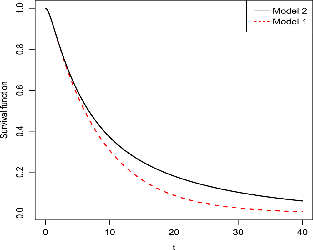
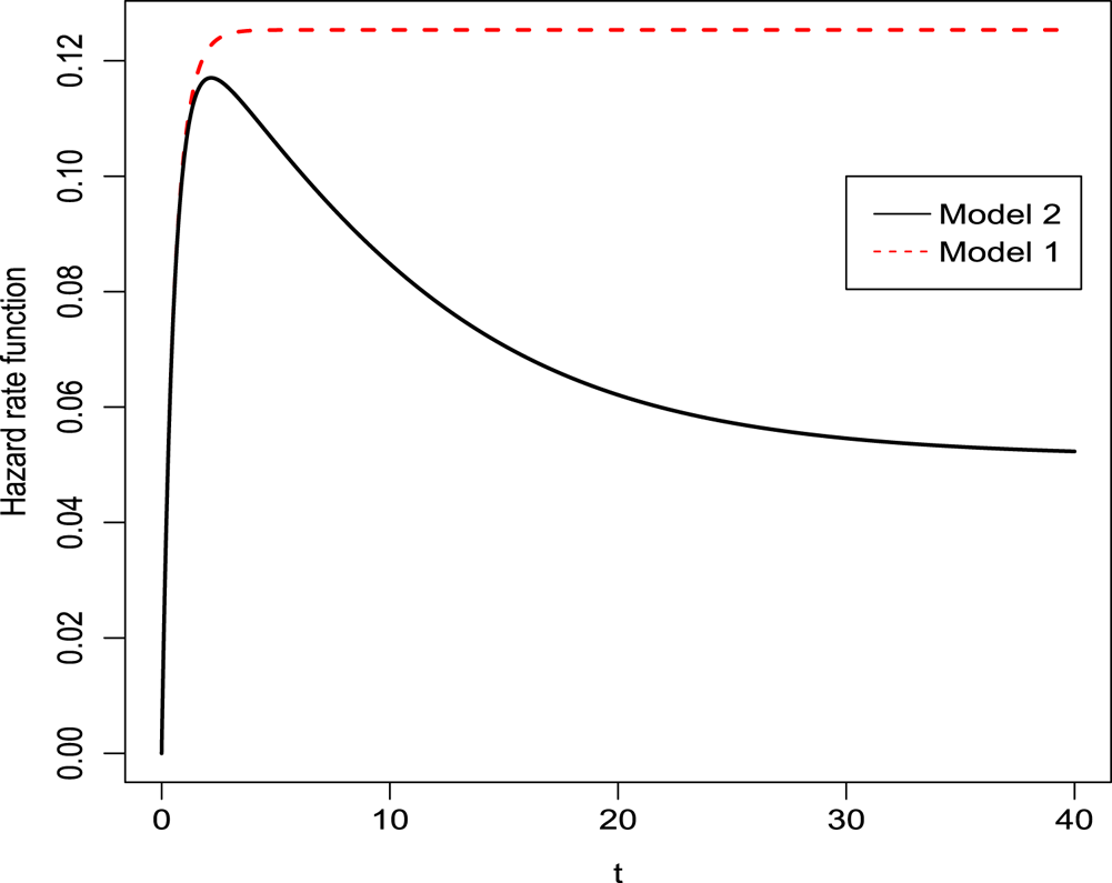
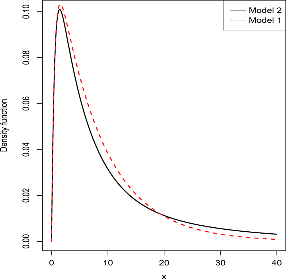
 $p_3=0.4$. In Figures 1, 2 and 4, we plot the survival functions, hazard rate functions and density functions of the system lifetime under Models 1 and 2. As expected, the survival function of
 $T_{1, {\mathbf {p}}}$ is a lower bound for that of
 $T_{2, {\mathbf {p}}}$ and the hazard rate of
 $T_{1, {\mathbf {p}}}$ is larger than that of
 $T_{2, {\mathbf {p}}}$. From Figure 4, we observe that the distribution of
 $T_{2,{\mathbf {p}}}$ is heavier tailed than that of
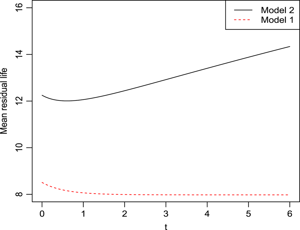
 $T_{1,{\mathbf {p}}}$, consistent with Theorem 2.5. From Figure 3, we also observe that the mean residual lifetime of
 $T_{2,{\mathbf {p}}}$ is greater than
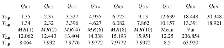
 $T_{1,{\mathbf {p}}}$ which is a consequence of the hr order proved in Theorem 2.3. In Table 1, we also derive some characteristic values of distributions of
 $T_{1,{\mathbf {p}}}$ and
 $T_{2,{\mathbf {p}}}$, such as
 $\alpha {\rm th}$ quantile (denoted by
 $Q_\alpha$), variance (denoted by
 ${{\mathbb {V}\mathrm {ar}}}$) and mean residual lifetime (denoted by
 $MR(t)$). We see that the
 $Q_{\alpha }$ for
 $T_{2,{\mathbf {p}}}$ is greater than
 $T_{1,{\mathbf {p}}}$ which explains the st order proved in Theorem 2.2. The mean for
 $T_{2,{\mathbf {p}}}$ is about
 $50\%$ larger than that of
 $T_{1,{\mathbf {p}}}$, and the standard deviation is almost double.
The plot of survival function of a system lifetime under Models 1 and 2

The plot of hazard rate function of a system lifetime under Models 1 and 2

The plot of mean residual function of a system lifetime under Models 1 and 2

The plot of density function of a system lifetime under Models 1 and 2

Some distribution characteristic values of  $T_{1, {\mathbf {p}}}$ and
 $T_{2, {\mathbf {p}}}$ in Example 2.1.

Remark 2.1. Let  $X$ and
 $Y$ be two non-negative random variables with density functions
 $f$ and
 $g$ and distribution functions
 $F$ and
 $G$, respectively. The random variable
 $X$ is said to be less dispersed than the random variable
 $Y$ (denoted by
 $X\le _{{\rm disp}} Y$) if
 $F^{-1}(\beta ) - F^{-1}(\alpha ) \le G^{-1}(\beta ) - G^{-1}(\alpha )$, for
 $0\le \alpha \le \beta \le 1$ where
 $G^{-1}$ and
 $F^{-1}$ are the right continuous inverses of
 $G$ and
 $F$, respectively. It is proved in Shaked [Reference Shaked19] that if
 $X\le _{{\rm st}} Y$ and for all
 $c>0$,
 $f(x-c)-g(x)$ has at most two sign changes with the sign sequence
 $- , + , -$ in case of two sign changes, then
 $X\le _{{\rm disp}}Y$. In Example 2.1, from the enters in Table 1, we observe that the difference between any two quantiles of
 $T_{1, {\mathbf {p}}}$ is less than that of
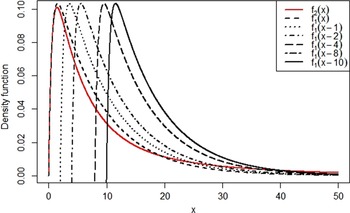
 $T_{2, {\mathbf {p}}}$. In Figure 5, we also observe that the sign change of
 $f_{1}(x-c)- f_{2}(x)$ for
 $c=0, 1, 2, 4, 6, 10$ is at most two with the sign sequence
 $- , + , -$ in case of two sign changes, where
 $f_i$,
 $i=1,2$, is the density function of
 $T_{i, {\mathbf {p}}}$. Thus, we conjecture that
 $T_{1, {\mathbf {p}}}\le _{{\rm disp}} T_{2, {\mathbf {p}}}$ if the inter-arrival times are IFR, which is stronger than variance order proved in Theorem 2.5.
The plot of  $f_2(x)$ and
 $f_1(x-c)$ for
 $c=0,1, 2, 4, 8, 10.$

Let  $N_{2, {\mathbf {p}}}$ be the number of shocks that cause the failure of the system in Model 2 with
 ${\mathbf {p}}=(p_1, \ldots, p_m)$. It is easy to see that if
 ${\mathbf {p}}\le _{m} {\mathbf {p}}^{*}$, then
 $N_{2,\mathbf {p}}\le _{{\rm st}} N_{2, {\mathbf {p}}^{*}}$. In the following theorem, for the case when
 $m = 2$ and
 $\pi _1=\pi _2=\frac 12$, the
 $\rm st$ order can be replaced by the
 $\rm hr$ order.
Theorem 2.6. Let  $N_{2, {\mathbf {p}}}$ be the number of shocks that cause the failure of the system in Model 2, where
 ${\mathbf {p}}=(p_1, \ldots, p_m)$. Then, for
 $m=2$ and
 $\pi _1=\pi _2$,
 $$(p_1, p_2)\le_{m} (p^{*}_1, p^{*}_2) \Longrightarrow N_{2, {\mathbf{p}}}\le_{{\rm hr}}N_{2, {\mathbf{p}^{*}}}.$$
Proof. Using implication (1.1) and Lemma 1.1, we need to show that for  $0\le p^{*}\le p\le c/2\le 1$,
 $$\frac{(1-p^{*})^{n+1}+(1-c+p^{*})^{n+1}}{(1-p)^{n+1}+(1-c+p)^{n+1}}\ge \frac{(1-p^{*})^{n}+(1-c+p^{*})^{n}}{(1-p)^{n}+(1-c+p)^{n}}$$
which is equivalent to
 \begin{align} & (1-p)^{n}(1-p^{*})^{n}(p-p^{*}) - (1-c+p)^{n}(1-c+p^{*})^{n}(p-p^{*})\nonumber\\ & \qquad +(1-p^{*})^{n}(1-c+p)^{n}(c-p-p^{*}) - (1-p)^{n}(1-c+p^{*})^{n}(c-p-p^{*}) \nonumber\\ & \quad = ((1-p)^{n}(1-p^{*})^{n}-(1-c+p)^{n}(1-c+p^{*})^{n})(p-p^{*}) \nonumber\\ & \qquad + ((1-p^{*})^{n}(1-c+p)^{n}-(1-p)^{n}(1-c+p^{*})^{n})(c-p-p^{*}) \ge 0. \end{align}
The first term in (2.3) is non-negative since  $p^{*}\le p\le c/2$,
 $1-p\ge 1-c+p$ and
 $1-p^{*}\ge 1-c+p^{*}$. The second term in (2.3) is non-negative since
 ${(1-p)}/{(1-c+p)}$ is a decreasing function in
 $p$ and
 $(c-p-p^{*})\ge 0$.
Next, a counterexample is given to illustrate that the result of Theorem 2.6 might not hold for  $m>2$.
Example 2.2. Let  $\bar {F}_{N_{2, {\mathbf {p}}}}(n)$ denote the survival function of
 $N_{2, \mathbf {p}}$. For
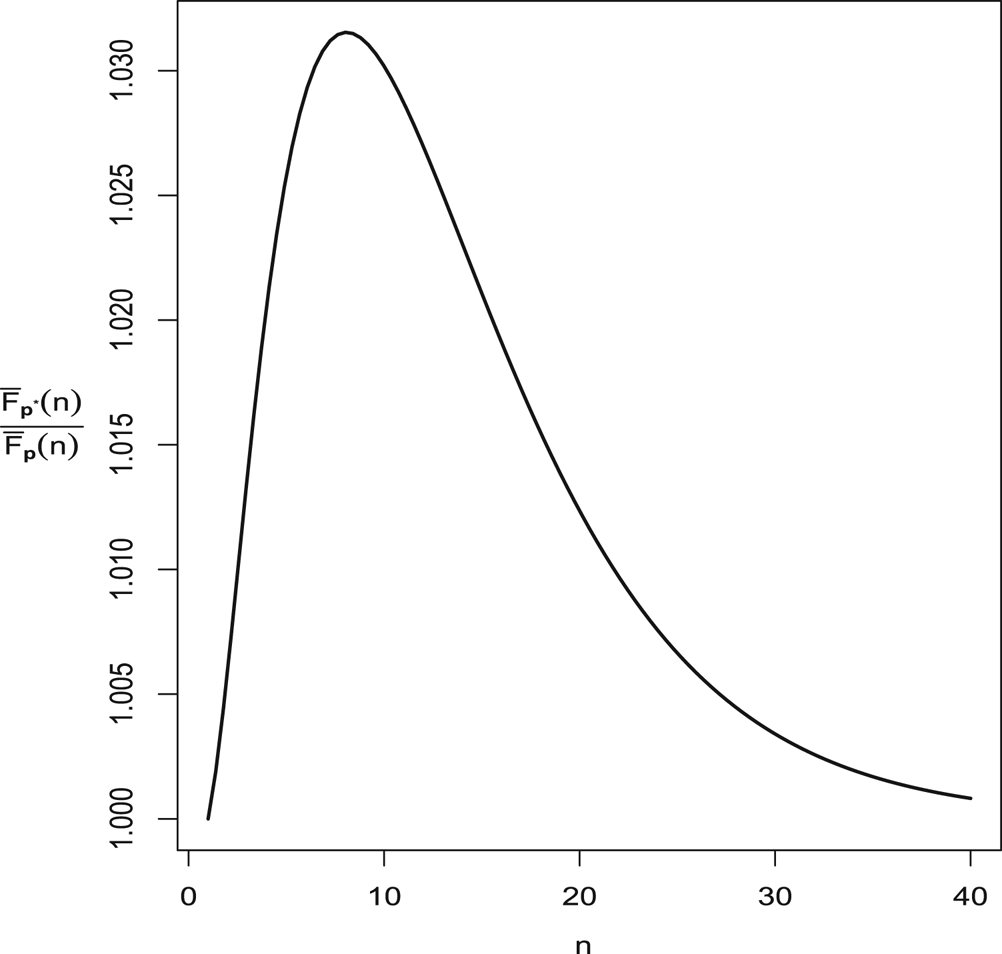
 ${\mathbf {p}}=(\frac 28, \frac 38, \frac 58)\le _{m}(\frac 28,\frac {2.9}8,\frac {5.1}8)={\mathbf {p}}^{*}$,
 ${\bar {F}_{N_{2, {\mathbf {p}^{*}}}}(5)}/{\bar {F}_{N_{2, \mathbf {p}}}(5)}=1.025786$,
 ${\bar {F}_{N_{2, {\mathbf {p}^{*}}}}(10)}/{\bar {F}_{N_{2, {\mathbf {p}}}}(10)}=1.030184$ and
 ${\bar {F}_{N_{2, {\mathbf {p}^{*}}}}(20)}/{\bar {F}_{N_{2, \mathbf {p}}}(20)}=1.012353$, which indicate that
 ${\bar {F}_{N_{2, {\mathbf {p}^{*}}}}(n)}/{\bar {F}_{N_{2, \mathbf {p}}}(n)}$ is not increasing (see also Figure 6).
The plot of  ${\bar {F}_{N_{2,{\mathbf {p}^{*}}}}(n)}/{\bar {F}_{N_{2, {\mathbf {p}}}}(n)}$ for
 ${\mathbf {p}}=(\frac 28, \frac 38, \frac 58)$ and
 ${\mathbf {p}}^{*}=(\frac 28,\frac {2.9}8,\frac {5.1}8)$.

The following theorem discusses the usual stochastic ordering of  $N_{2, {\mathbf {p}}}$ and
 $N_{2, {\mathbf {p}}}$ when
 ${\mathbf {p}}$ and
 ${\mathbf {p}}^{*}$ are component-wise ordered. The result follows from the observation that the survival function of
 $N_{2, {\mathbf {p}}}$ is decreasing in
 $p_i$,
 $i=1, \ldots, m$.
Theorem 2.7. If  $p^{*}_i\le p_i$,
 $i=1, \ldots, m$, then
 $N_{2, {\mathbf {p}}}\le _{{\rm st}} N_{2, {\mathbf {p}}^{*}}$.
The following counterexample shows that the result of the above theorem can not be extended to the hazard rate order.
Example 2.3. Let  $\bar {F}_{N_{2, {\mathbf {p}}}}(n)$ denote the survival function of
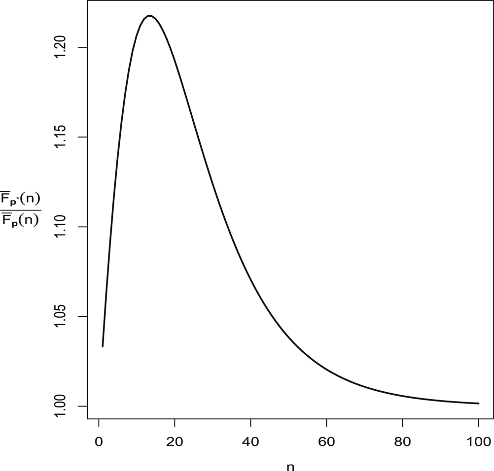
 $N_{2, { \mathbf {p}}}$. In Figure 7, we plot
 ${\bar {F}_{N_{2, {\mathbf {p}^{*}}}}(n)}/{\bar {F}_{N_{2, \mathbf {p}}}(n)}$ for
 ${\mathbf {p}}=(0.2, 0.3)$,
 ${\mathbf {p}}^{*}=(0.2, 0.25)$ and
 $\pi _1=\pi _2$. The figure shows that the condition
 $p^{*}_i\le p_i$,
 $i=1, \ldots, m$ does not imply
 $N_{2, {\mathbf {p}}}\le _{{\rm hr}} N_{2, {\mathbf {p}}^{*}}$.
The plot of  ${\bar {F}_{N_{2, {\mathbf {p}^{*}}}}(n)}/{\bar {F}_{N_{2,{\mathbf {p}}}}(n)}$ for
 ${\mathbf {p}}=(0.2, 0.3)$ and
 ${\mathbf {p}}^{*}=(0.2,0.25)$.

The following theorem deals with the stochastic behaviour of  $N_{2, {\mathbf {p}}}$ with respect to
 ${\bf \pi }=(\pi _1, \ldots, \pi _m)$.
Theorem 2.8. In Model 2, let  $N^{\bf \pi }_{2, {\mathbf {p}}}$ denote the number of shocks that cause the failure of the system with
 ${\bf \pi }=(\pi _1, \ldots, \pi _m)$. Then under the condition
 $p_1\ge p_2\ge \cdots \ge p_m$,
(a)
${\bf \pi }\le _{{\rm st}}{\bf \pi }^{*} \Longrightarrow N^{\bf \pi }_{2, {\mathbf {p}}}\le _{{\rm st}}N^{{\bf \pi }^{*}}_{2, {\mathbf {p}}}$.(b)
${\bf \pi }\le _{{\rm hr}}{\bf \pi }^{*} \Longrightarrow N^{\bf \pi }_{2, {\mathbf {p}}}\le _{{\rm hr}}N^{{\bf \pi }^{*}}_{2, {\mathbf {p}}}$.(c)
${\bf \pi }\le _{{\rm lr}}{\bf \pi }^{*} \Longrightarrow N^{\bf \pi }_{2, {\mathbf {p}}}\le _{{\rm lr}}N^{{\bf \pi }^{*}}_{2, {\mathbf {p}}}$.


Proof. The probability mass function of  $N^{\bf \pi }_{2, {\mathbf {p}}}$ is given by
 $$\mathbb{P}(N^{\bf\pi}_{2, {\mathbf{p}}}=n)=\sum_{i=1}^{m}\pi_i p_i (1-p_i)^{n-1}, \quad n=1, 2, \ldots.$$
It is a mixture of geometric distributions. Now, the required results of  $a$,
 $b$ and
 $c$ follow, respectively, from Theorems 1.A.6, 1.B.14 and 1.C.17 in Shaked and Shanthikumar [Reference Shaked and Shanthikumar20].
The result of the next theorem follows from Theorem 2.8 and Theorems 1.A.4, 1.B.7 and 1.C.11 in Shaked and Shanthikumar [Reference Shaked and Shanthikumar20].
Theorem 2.9. In Model 2, let  $T^{\bf \pi }_{2, {\mathbf {p}}}$ be the system lifetime with
 ${\bf \pi }=(\pi _1, \ldots, \pi _m)$. Then under the condition
 $p_1\ge p_2\ge \cdots \ge p_m$,
(a)
${\bf \pi }\le _{{\rm st}}{\bf \pi }^{*}$ implies $T^{\bf \pi }_{2, {\mathbf {p}}}\le _{{\rm st}}T^{{\bf \pi }^{*}}_{2, {\mathbf {p}}}$ when the inter-arrival times of consecutive shocks are independent.(b)
${\bf \pi }\le _{{\rm hr}}{\bf \pi }^{*}$ implies $T^{\bf \pi }_{2, {\mathbf {p}}}\le _{{\rm hr}}T^{{\bf \pi }^{*}}_{2, {\mathbf {p}}}$ when the inter-arrival times of consecutive shocks are independent with IFR property.(c)
${\bf \pi }\le _{{\rm lr}}{\bf \pi }^{*}$ implies $T^{\bf \pi }_{2, {\mathbf {p}}}\le _{{\rm lr}}T^{{\bf \pi }^{*}}_{2, {\mathbf {p}}}$ when the inter-arrival times of consecutive shocks are independent with log-concave density.


3. Age replacement policy
The age replacement policy is a commonly utilized strategy for preventing the costly breakdown of a system or a component during an operation. In an age replacement policy, the system is replaced at the time of failure or at a pre-specified time  $\tau$ if it is operational at time
 $\tau$. Let
 $T$ denote the system lifetime with distribution function
 $F$ and let
 $c_1$ and
 $c_2$ represent the replacement costs of each failed and non-failed item, respectively. We assume that
 $c_2< c_1$ since a failure carries an additional penalty. For the replacement time
 $\tau$, the expected cost rate is defined as
 \begin{equation} C(\tau)=\frac{\text{Expected cost of one cycle}}{\text{Expected time of one cycle}}=\frac{c_1F(\tau) + c_2 \bar{F}(\tau)}{{{\mathbb{E}}}(\min\{T, \tau\})} \end{equation}
(cf. Nakagawa [Reference Nakagawa16]).
The optimal replacement time denoted by  $\tau ^{*}$ is a time that the expected cost rate has the lowest value, that is,
 $$C(\tau^{*})=\min_{\tau>0} C(\tau).$$
The expected cost rate of age replacement policy for Model  $i$,
 $i=1, 2$, is given by
 $$C_i(\tau)= \frac{c_1 - (c_1-c_2)\bar{F}_i(\tau)}{{{\mathbb{E}}}(\min\{T_{i, {\mathbf{p}}}, \tau\})}$$
where  $F_i$ is the distribution function of
 $T_{i, {\mathbf {p}}}$. Since
 $\min \{t,\tau \}$ is an increasing function of
 $t$,
 $T_{1, {\mathbf {p}}}\le _{{\rm st}} T_{2, {\mathbf {p}}}$ implies that
 ${{\mathbb {E}}}(\min \{T_{1, {\mathbf {p}}}, \tau \})\le {{\mathbb {E}}}(\min \{T_{2, {\mathbf {p}}}, \tau \})$, for
 $\tau >0$. Combining this observation with the fact that
 $\bar {F}_1(\tau ) \le \bar {F}_2(\tau )$ (Theorem 2.2), we conclude that
 $$C_2(\tau)\le C_1(\tau), \quad \forall \tau>0.$$
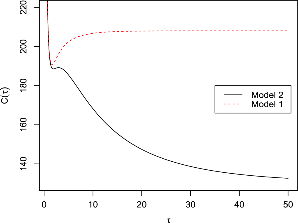
That is, for any pre-specified age replacement time  $\tau$, the expected cost rate for Model 1 is larger than that of Model 2. Now, let
 $\tau _1^{*}$ and
 $\tau ^{*}_2$ be the optimal age replacement times under Models 1 and 2, respectively. Then,
 $$C_2(\tau^{*}_2)\le C_2(\tau^{*}_1)\le C_1(\tau^{*}_1).$$
Suppose that a system is subject to a sequence of shocks that come from three sources with probability  $\pi _1=0.2, \pi _2= 0.5$ and
 $\pi _3=0.3$. Assume that the times between two consecutive shocks have Erlang distribution with shape parameter
 $2$ and rate parameter
 $0.8$. It is also assume that
 $p_1=0.5$,
 $p_2=0.75$ and
 $p_3=0.15$, and
 $c_1=1000$ and
 $c_2=100$. In Figure 8, we plot
 $C_1(\tau )$ and
 $C_2(\tau )$ (see [Reference Bozbulut and Eryilmaz2,Reference Eryilmaz3] to compute the expected cost rate function). The figure justifies that
 $C_2(\tau ) \le C_1(\tau )$ for all
 $\tau >0$. The hazard rate function of
 $T_{1}$, denoted by
 $r_{T_{1}}(t)$, is increasing and
 $r_{T_{1}}(\infty )>{c_1}/[{E(T_{1})(c_1-c_2)}]=0.231$. Using these observations, it follows from Theorem 3.2 of Nakagawa [Reference Nakagawa16], the optimal replacement time is finite and unique which is equal to
 $\tau ^{*}_1=1.938$ with
 $C_1(\tau ^{*}_1)=190.83$. On the other hand, the hazard rate function of
 $T_{2}$ is not increasing and the optimal replacement time of Model 2 is
 $\tau ^{*}_2=\infty$ with
 $C_2(\tau ^{*}_2)={c_1}/{{{\mathbb {E}}}(T_2)}=130.4348$, since
 $C_2(\tau )$ is decreasing for
 $\tau >2.950$.
The plot of the expected cost rate for Models 1 and 2 with  ${\bf \pi }=(0.2, 0.5, 0.3)$ and
 ${\mathbf {p}}=(0.5, 0.75, 0.15)$.

Acknowledgments
The authors would like to thank the Associate Editor and the reviewer for their valuable comments and suggestions, which definitely improved the quality and presentation of the paper. We thank Professor Hassan Zahedi-Jasbi for his valuable inputs and comments that strengthened the manuscript.