

1. Introduction
The development of instabilities in shear flows depends on whether the instability is convective or absolute. In the case of a convective instability, small growing perturbations travel downstream, and nonlinear effects, either secondary instability or transition to turbulence, manifest themselves further downstream from the point where the instability was initiated. Segments of such flows, even unstable ones, can be observed in reality, e.g. plane Poiseuille flow and Blasius boundary layer, whose convective nature of instability was proved by Deissler (Reference Deissler1987) and Brevdo (Reference Brevdo1995) for moderate  $Re$, and by Iordanskii & Kulikovskii (Reference Iordanskii and Kulikovskii1966) for asymptotically large
 $Re$. If the instability is absolute, then growing perturbations occupy region spreading both upstream and downstream, thus making impossible the observation of the unstable flow in reality.
The instability nature of constant-density plane mixing layers was independently studied first by Huerre & Monkewitz (Reference Huerre and Monkewitz1985) and Shikina (Reference Shikina1987); they proved that the instability can be absolute only in the presence of a certain amount of counter-flow, whereas a unidirectional shear layer is unstable convectively. Monkewitz & Sohn (Reference Monkewitz and Sohn1988) analysed the instability of round compressible jets and showed that it can be absolute only if the jet is sufficiently light, i.e. either the jet is hot, or it consists of a gas that is lighter than the ambient medium so that their density ratio is smaller than a certain critical value. Compressibility and viscosity effects can only decrease the critical density ratio (Lesshafft & Huerre Reference Lesshafft and Huerre2010). The local absolute instability yields the global instability of a spatially developing low-density jet, as demonstrated by Coenen et al. (Reference Coenen, Lesshafft, Garnaud and Sevilla2017). The effect of velocity profiles of jets flowing out of tubes of different lengths was studied by Coenen, Sevilla & Sánchez (Reference Coenen, Sevilla and Sánchez2008), and the critical density ratio is also less than unity in all cases. Jendoubi & Strykowski (Reference Jendoubi and Strykowski1994) analysed the instability nature of jets in the presence of external flow; in particular, it was shown that the modes resulting in absolute instability in light jets (Monkewitz & Sohn Reference Monkewitz and Sohn1988), and in constant-density jets or shear layers with counter-flow (Huerre & Monkewitz Reference Huerre and Monkewitz1985; Shikina Reference Shikina1987), are actually two different modes. Further analysis of two coaxial co-flowing jets, which have two shear layers and two interplaying absolute instability modes, was performed by Balestra, Gloor & Kleiser (Reference Balestra, Gloor and Kleiser2015).
Experiments with low-density jets (Monkewitz et al. Reference Monkewitz, Bechert, Barsikow and Lehmann1990; Kyle & Sreenivasan Reference Kyle and Sreenivasan1993; Strykowski, Krothapalli & Jendoubi Reference Strykowski, Krothapalli and Jendoubi1996; Hallberg et al. Reference Hallberg, Srinivasan, Gorse and Strykowski2007; Li & Juniper Reference Li and Juniper2013) confirm that the jet dynamics is changed drastically when crossing the absolute-versus-convective instability boundary: global jet oscillations and strong side jets appear; further downstream, the flow blows up and does not even look like a jet. A recent study of Demange, Chazot & Pinna (Reference Demange, Chazot and Pinna2020) considers realistic flow profiles observed in plasma jets, and demonstrates a large portion of absolutely unstable flow, which explains single-frequency oscillations observed in experiment.
It is interesting to note that in contrast to round jets, a plane unidirectional mixing layer stays convectively unstable for moderate density ratios, as shown by Pavithran & Redekopp (Reference Pavithran and Redekopp1989) and Jackson & Grosch (Reference Jackson and Grosch1990) (they assumed different temperature distributions), and switches to absolute instability only at very small density ratios, much smaller than in round jets (Caillol Reference Caillol2008, see his figure 3). The presence of a wake behind a splitter plate in a plane mixing layer can also trigger the absolute instability, as shown by Lee & Morris (Reference Lee and Morris1997).
A series of studies is devoted to the instability nature of wakes, motivated by the explanation of the onset of the von Kármán vortex street in the cylinder wake. Monkewitz (Reference Monkewitz1988) considered a family of wake profiles and performed a viscous analysis of the instability nature. By matching the profile parameters with the wakes observed behind a cylinder, he found that local absolute instability takes place at  $Re^D>25$ (where
 $Re^D$ is the Reynolds number based on the cylinder diameter and upstream velocity), i.e. before the onset of the von Kármán vortex street occurring at
 $Re^D>47$. The latter can be interpreted as the evolution of a linear global mode that grows when the local absolute instability region becomes sufficiently long (Pier Reference Pier2002). Although the main implication was the evolving wake behind a cylinder, in the context of the present study, we note that Monkewitz (Reference Monkewitz1988) demonstrated an absolute instability of a unidirectional wake (i.e. wake without counter-flow) for
 $Re>11.3$.
Delbende & Chomaz (Reference Delbende and Chomaz1998) analysed the role of nonlinear effects by performing fully nonlinear direct numerical simulations of the localized perturbation evolution to a plane-parallel wake with the same velocity profile as considered by Monkewitz (Reference Monkewitz1988). They found that although the wave packet is rapidly saturated and the exponential growth is limited by strong nonlinear terms, velocities of both upstream and downstream edges of the nonlinear wave packet are still governed by the linear spatiotemporal instability analysis.
Juniper (Reference Juniper2006, Reference Juniper2007) analysed plane jet/wake plug and piecewise-linear velocity profiles, and studied the effect of the flow confinement. He showed that the confinement yields the appearance of additional saddle points near the negative imaginary wavenumber ray, which drive the absolute instability at specific parameters. Moreover, the change of confinement ratio changes the governing saddle points. It is interesting that specific confinement ratios enhance the absolute instability compared to the unconfined case. In particular, the varicose mode of the constant-density unidirectional jet touches the absolutely instability boundary at a certain confinement ratio. This analysis of plane flows was extended to the axisymmetric configuration by Juniper (Reference Juniper2008). Similar conclusions were made for round jets/wakes: the absolute instability is enhanced for moderate confinement ratios.
Further progress was made by Rees & Juniper (Reference Rees and Juniper2010), who included smooth velocity profiles and non-zero viscosity in the analysis. The touch of the absolute instability boundary by the unidirectional plug jet profile (Juniper Reference Juniper2006) turns into the penetration into the absolute instability region for a smooth unidirectional confined jet for specific velocity distributions. That is, there exist unidirectional confined jets that are absolutely unstable. When the viscosity is taken into account, the instability nature turns into convective for  $Re<1000$.
Mathematical insight into the role of confinement was provided by Healey (Reference Healey2009), who studied analytically the nature of instability of mixing layers. Namely, the clue is in the behaviour of the complex wavenumber  $\alpha$-plane in the vicinity of a negative imaginary ray. When the flow is unconfined (i.e. a decaying boundary condition is set as transverse coordinate
 $y\to \pm \infty$), this ray has no saddle points in its vicinity. The nature of the instability is driven by a saddle point lying in the fourth quadrant of the
 $\alpha$-plane:
 ${\rm Re}\,\alpha _s>0$,
 ${\rm Im}\alpha _s<0$. However, when the flow is confined, the decaying condition is substituted by the free-slip condition at the walls, which yields the appearance of an infinite discrete set of poles along the negative imaginary
 $\alpha$ ray. Near each pole, there exists a saddle point. For specific confinements, the upper of those saddle points becomes dominating, i.e. governing the instability nature. Moreover, this saddle point can stay dominating in the limit of weak confinements: walls moving towards infinity. In other words, unconfined flow and the flow confined by walls located arbitrarily far in the transverse direction have different absolute instability criteria. This explains why absolute instability of jets and mixing layers, being possible for the unconfined flow only in the presence of the counter-flow, exists for the confined flow even in the unidirectional flow case.
This behaviour resembles the analogous situation with the stability criterion of arbitrarily long but finite-length systems (Kulikovskii Reference Kulikovskii1966, Reference Kulikovskii2006), which (in general) differs from the stability criterion for an infinitely long system. Physically, in both cases the difference between the asymptotic bounded problem and the unbounded problem is in the reflection of waves from the walls in the bounded case that admits eigenmodes non-existing in the unbounded case.
It should be noted that the co-flow absolute instability of the confined jets and mixing layers is associated with non-decaying behaviour of perturbations in the transverse direction. In real flows, which are always limited in length, the absolutely unstable mode will need for realization an axial length much longer than the transverse distance between walls. It is natural to expect that the laminar flow will break up at sufficiently large axial distance so that the absolutely unstable mode will also be destroyed. In other words, if the confinement is weak, then only such modes can be realized that satisfy the decaying condition. In this sense, there is no hope that the absolute instability of weakly confined jets or mixing layers can be observed in reality.
Biancofiore & Gallaire (Reference Biancofiore and Gallaire2011) included the confinement in the wake profiles considered before by Monkewitz (Reference Monkewitz1988) in the unconfined case. They removed the gap between Monkewitz (Reference Monkewitz1988), who predicted absolute instability of specific smooth unconfined co-flow wakes, and Juniper (Reference Juniper2006, Reference Juniper2007), who obtained convective instability of plug and piecewise-linear co-flow wakes (both unconfined and weakly confined). Namely, Biancofiore & Gallaire (Reference Biancofiore and Gallaire2011) showed how the change of the profile parameter switches absolute instability to convective for a weakly confined wake. However, the most effective enhancement of the absolute instability obtained by Juniper (Reference Juniper2006, Reference Juniper2007) at the confinement ratio  $h\approx 1$ is observed for all considered smooth velocity profiles, i.e. it is not affected by the inclusion of a shear layer into the velocity profile.
A tougher test of the confinement effect was performed by Biancofiore, Gallaire & Pasquetti (Reference Biancofiore, Gallaire and Pasquetti2011), who analysed global oscillations in a realistic, spatially evolving, finite-length viscous confined wake. Base flow was calculated as a solution of Navier–Stokes equations with incoming plug velocity profile. After introduction of a random perturbation, its evolution was calculated by direct numerical simulations. Depending on the confinement and velocity ratios, the perturbation was either carried away by the flow, or transformed into global oscillations. For  $Re=100$, the range of parameters where global oscillations were set was qualitatively similar to those obtained by Juniper (Reference Juniper2006) as the region of local absolute instability. In particular, the largest enhancement of the absolute instability, as well as of global oscillations, occurred at the confinement ratio
 $h\approx 1$. However, for
 $Re=500$, Biancofiore et al. (Reference Biancofiore, Gallaire and Pasquetti2011) also found a different type of global oscillations, called a ‘front vacillation instability’, which has no relation to local instability nature.
As follows from the reviewed studies, for constant-density unconfined non-swirling round jets or plane mixing layers with classical velocity profiles without counter-flow, the instability is convective. However, recently, based on inviscid-flow analysis, it was shown independently by Lesshafft & Marquet (Reference Lesshafft and Marquet2010), Balestra et al. (Reference Balestra, Gloor and Kleiser2015) and Vedeneev & Zayko (Reference Vedeneev and Zayko2018) that for specific, non-classical velocity profiles, the instability can be absolute even for the constant-density unconfined jets without counter-flow. Namely, such profiles should have sufficiently small velocity and large velocity slope at the inflection point. Physically, these conditions provide small phase speed and large growth rate of the growing mode, which are necessary for the onset of absolute instability.
In the present study, we consider the case of two-dimensional plane jets of incompressible fluid. To make sure that the interacting spatial waves are selected correctly, in § 2 we start with the inviscid analysis of the classical shear layer studied before by Huerre & Monkewitz (Reference Huerre and Monkewitz1985) and Shikina (Reference Shikina1987), and use saddle-point analysis to determine the nature of the instability (Briggs Reference Briggs1964; Bers Reference Bers1983). Next, after switching to the case of jets, in § 3 we consider the family of two-parameter smooth velocity profiles. We show that similarly to round jets, the instability becomes absolute when at the inflection point either the velocity is small, or its slope is large. We detect critical parameter values corresponding to the switch between absolute and convective instability. In § 4, we perform viscous analysis of the profiles that are absolutely unstable in the inviscid limit, and calculate the values of the Reynolds number corresponding to the switch between absolute and convective instability. To perform an independent verification of the saddle-point analysis, in § 5 we conduct direct numerical calculations of the growth of a localized perturbation in the framework of linearized Navier–Stokes equations. Our calculations are similar to those of Delbende, Chomaz & Huerre (Reference Delbende, Chomaz and Huerre1998), where the development of an impulse perturbation in a Batchelor vortex was investigated. Using Fourier and Hilbert transformations, Delbende et al. (Reference Delbende, Chomaz and Huerre1998) were able to determine the growth rate and the dominant values of the wavenumber and frequency of perturbation along each of the rays in the spatiotemporal plane, depending on the value of the rotation parameter and the magnitude of the external flow. As we are interested only in the absolute/convective instability, in this paper we limit ourselves to determination of the perturbation growth rate at a fixed spatial point. We show that the back edge of the perturbation travels downstream for subcritical  $Re$, and upstream for supercritical
 $Re$, thus confirming results of the saddle-point analysis. Finally, in § 6, we discuss possible applications of the present findings and conclude the paper.
2. The inviscid instability of the classical velocity profile and of its parametrized approximation
2.1. Governing equations and boundary conditions
We analyse hydrodynamic stability of a two-dimensional (plane) shear flow with velocity distribution  $(U,V)$, with
 $U=U(y)$,
 $V=0$. The problem is non-dimensionalized with maximum positive velocity and shear layer thickness, or half the jet width, taken as velocity and length scales. By considering perturbation dependence on
 $x$ and
 $t$ in the travelling-wave form,
 $\sim {\rm e}^{{\rm i} (\alpha x-\omega t)}$, and substituting into linearized Navier–Stokes equations, a well known Orr–Sommerfeld equation for the amplitude of
 $y$-perturbation component
 $v(y)$ is obtained:
 \begin{equation} \frac{1}{{\rm
i}\,Re\,\alpha}\left(\frac{{\rm d}^4 v}{{{\rm d}
y}^4}-2\alpha^2\,\frac{{\rm d}^2 v}{{{\rm d} y}^2}+\alpha^4
v\right)= \frac{{\rm d} }{{\rm d} y}\left((U-c)\,\frac{{\rm d} v}{{\rm d} y}- v\, \frac{{\rm d} U}{{\rm d} y}\right)-\alpha^2(U-c) v,
\end{equation}
where  $\alpha$ and
 $\omega$ are the wavenumber and frequency, and
 $c=\omega /\alpha$ is the phase speed.
To consider eigenmodes of the shear flow, we must impose a decaying boundary condition, i.e.  $v(y)\to 0$ as
 $y\to \pm \infty$. For the purpose of the numerical analysis, it is convenient to transfer this asymptotic boundary condition to sufficiently remote stations
 $y=L_-,L_+$ in the following manner. For large
 $|y|$, the base velocity is
 $U(y)\approx U_{lim}$, and the Orr–Sommerfeld equation is rewritten as an equation with constant coefficients:
 \begin{equation} \frac{1}{{\rm i} \,Re\,\alpha}\left(\frac{{\rm d}^2 }{{{\rm d} y}^2}-\alpha^2\right)^2 v+ (c-U_{lim})\left(\frac{{\rm d}^2 }{{{\rm d} y}^2}-\alpha^2\right) v=0. \end{equation}
Hence its general solution is
 \begin{equation} v(y)=\sum_{j=1}^4 C_j\,v_j(y), \end{equation}
where
 \begin{equation} v_1={\rm e}^{\alpha y},\quad v_2={\rm e}^{-\alpha y},\quad v_3={\rm e}^{\lambda y},\quad v_4={\rm e}^{-\lambda y},\quad \lambda=\sqrt{-{\rm i} \,Re}\,\sqrt{\omega-U_{lim}\alpha-\frac{\alpha^2}{{\rm i} \,Re}}. \end{equation}
Assuming, without loss of generality, that  ${\rm Re}\,\alpha >0$,
 ${\rm Re}\,\lambda >0$, we eliminate exponentially growing components by setting
 $C_1=C_3=0$ as
 $y\to +\infty$, and
 $C_2=C_4=0$ as
 $y\to -\infty$. Among the two remaining decaying exponents, say
 $v_2(y)$ and
 $v_4(y)$ for
 ${y\to +\infty}$, the first one is leading, because they are rated as
 \begin{equation} \frac{v_4}{v_2}\sim \exp\left(-{\sqrt{Re}\, \sqrt{\frac{\omega-U_{lim}\alpha}{2}}}\,y\right),\end{equation}
which is an exponentially small number as  $y\to +\infty$. Hence we may ignore
 $v_4$ and put, with a negligible error,
 \begin{equation} v(y)\sim {\rm e}^{-\alpha y},\ y\to +\infty, \quad v(y)\sim {\rm e}^{\alpha y},\ y\to -\infty. \end{equation}
Next, we substitute the decaying boundary conditions with the condition of matching with the exponential solution (2.6a,b) at  $y=L_-, L_+$:
 \begin{equation} \frac{{\rm d} v}{{\rm
d} y}-\alpha v=0,\ \frac{{\rm d}^2 v}{{{\rm d} y}^2}-\alpha\,\frac{{\rm d} v}{{\rm d} y}=0, y=L_-, \quad
\frac{{\rm d} v}{{\rm d} y}+\alpha v=0,\ \frac{{\rm d}^2
v}{{{\rm d} y}^2}+\alpha\,\frac{{\rm d} v}{{\rm d} y}=0,
y=L_+.
\end{equation}
Values  $L_{\pm }$ must satisfy the condition
 $\sqrt {Re}\,|L_{\pm }|\gg 1$ (so the ratio (2.5) is small) and should be determined by a convergence study.
To start our analysis with a previously studied case of inviscid instability of the classical shear layer (Huerre & Monkewitz Reference Huerre and Monkewitz1985; Shikina Reference Shikina1987), first we will also consider inviscid stability analysis. In this case, taking the limit  $Re\to \infty$ in (2.1), we obtain the Rayleigh equation
 \begin{equation}
\frac{{\rm d}}{{\rm d} y}\left((U(y)-c)\,\frac{{\rm d} v}{{\rm d} y}-
v\,\frac{{\rm d} U(y)}{{\rm d} y}\right)-\alpha^2(U(y)-c)
v=0.\end{equation}
As this equation is of second order, it needs only two boundary conditions:
 \begin{equation} \frac{{\rm d} v}{{\rm d} y}-\alpha v=0, y=L_-, \quad \frac{{\rm d} v}{{\rm d} y}+\alpha v=0, y=L_+. \end{equation}
2.2. Numerical solution of the eigenvalue problem
To perform the spatial instability analysis, for each complex frequency  $\omega$, we find eigenvalue
 $\alpha (\omega )$ and eigenmode
 $v(y)$ that satisfy (2.1) and boundary conditions (2.7a,b) for the viscous case, or (2.8) and (2.9a,b) for the inviscid case.
For the inviscid case, the boundary condition at  $y=L_-$ selects one of two linearly independent solutions of (2.8). Consider a particular solution in the form
 \begin{equation} v_1(L_-)=1, \quad v_1'(L_-)=\alpha. \end{equation}
Treating these as initial conditions, we integrate the Rayleigh equation (2.8) from  $y=L_-$ to
 $y=L_+$ by the Runge–Kutta method, and calculate the function
 \begin{equation} g(\alpha)=v_1'(L_+)+\alpha\,v_1(L_+). \end{equation}
Zeros of  $g$ are the eigenvalues of the problem (2.8)–(2.9a,b), because both the equation and boundary conditions are satisfied. They are found iteratively by the secant method.
A similar reduction of the eigenvalue problem to iterative solutions of initial value problems is used in the viscous case. The differences are as follows. First, boundary conditions at  $y=L_-$ select two linearly independent solutions,
 $v_1(y)$ and
 $v_2(y)$, and both are integrated up to
 $y=L_+$. Second, during the integrations, because of the small parameter at the leading-order derivative in (2.1), the use of an orthonormalization technique is necessary (Shmidt & Hennigson Reference Shmidt and Hennigson2001, Appendix A.2). Finally, to satisfy the boundary conditions at
 $y=L_+$, we consider linear combination
 $c_1\,v_1(y)+c_2\,v_2(y)$, and the requirement of non-zero
 $c_1$,
 $c_2$ yields
 \begin{equation} g(\alpha)= \begin{vmatrix} v_1'(L_+)+\alpha\,v_1(L_+) & v_2'(L_+)+\alpha\,v_2(L_+)\\ v_1''(L_+)+\alpha\,v_1'(L_+) & v_2''(L_+)+\alpha\,v_2'(L_+) \end{vmatrix} =0.\end{equation}
The solution of this equation is found by the secant method without changes with respect to the inviscid case.
Based on a convergence study, the spatial step size of the Runge–Kutta method was set equal to  $1/300$ in both the inviscid and viscous cases.
For large  $L_+$,
 $g(\alpha )$ becomes small due to the smallness of
 $v'(L_+)$ and
 $v(L_+)$, even if the matching conditions (2.7a,b) are not satisfied. To improve the numerical accuracy,
 $g(\alpha )$ in (2.12) can be normalized by dividing by
 $v_1(L_+)\,v_2(L_+)$, and the eigenvalues are searched as zeros of the normalized function.
2.3. Classical velocity profile
We start our analysis with a shear layer profile analysed by Huerre & Monkewitz (Reference Huerre and Monkewitz1985) and Shikina (Reference Shikina1987):
 \begin{equation} U_{cl}(y)=\frac{1-R+2R\,\tilde{U}_{cl}(y)}{1+R},\quad \tilde{U}_{cl}(y)=\frac{1- \tanh(4(y-1/2))}{2}, \end{equation}
where  $\tilde {U}_{cl}(y)$ is a unidirectional velocity profile (
 $0<\tilde {U}_{cl}<1$), and the parameter
 $R$ defines the added counter-flow. Namely, as
 $y\to -\infty$, the velocity
 $U(y)$ tends to 1, and the velocity limit as
 $y\to +\infty$ depends on
 $R$. If
 $R=1$, then
 $U(+\infty )=0$ (unidirectional flow), and if
 $R\to +\infty$, then
 $U(+\infty )=-1$ (symmetrical flow), as shown in figure 1(a). For
 $1< R<+\infty$, the parameter defines the relative counter-flow velocity:
 \begin{equation} \frac{U(+\infty)}{U(-\infty)}=\frac{1-R}{1+R}. \end{equation}
Note that the notation  $R$ for the counter-flow parameter is established in the literature (e.g. Huerre & Monkewitz Reference Huerre and Monkewitz1985), and should not be confused with the Reynolds number
 $Re$.
(a) Classical and (b) spline-defined velocity profiles of the shear layer for  $R=1.0, 1.5, \infty$.

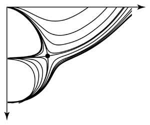
To perform the inviscid absolute instability analysis, we calculate the curves  $\alpha (\omega )$ in the complex
 $\alpha$-plane for real frequencies
 $\omega \in \mathbb {R}$. For
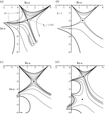
 $R=1$, two curves corresponding to two distinct eigenvalues
 $\alpha$ are found (figure 2a). The one located in the quadrant
 ${\rm Re}\,\alpha >0$,
 ${\rm Im}\,\alpha <0$ corresponds to the growing downstream-travelling mode, which is a usual Kelvin–Helmholtz mode; the other, located in the quadrant
 ${\rm Re}\,\alpha <0$,
 ${\rm Im}\,\alpha <0$, is an upstream-travelling decaying mode. When
 $R$ is increasing, the two curves approach each other and generate a saddle point
 $\omega (\alpha )$ at
 $R=R_{cr}=1.315$, which signifies the transition from convective to absolute instability, according to the absolute instability criterion (Briggs Reference Briggs1964; Bers Reference Bers1983). For
 $R>R_{cr}$, the curves are switched, and the instability stays absolute for any larger
 $R$. Note that as
 $R\to +\infty$, the absolute character of the instability is evident from the base flow symmetry.
Images of the  ${\rm Im}\,\omega =0$ line in the complex
 $\alpha$-plane, and transition between absolute and convective instability at increasing
 $R$. (a) Classical shear layer, (b) spline approximation of the shear layer, (c) symmetric mode of the jet, and (d) antisymmetric mode of the jet.

The critical value  $R_{cr}=1.315$ was calculated previously independently by Huerre & Monkewitz (Reference Huerre and Monkewitz1985) and Shikina (Reference Shikina1987); coincidence of our results validates the present analysis and selects two particular
 $\alpha (\omega )$ modes, whose collision yields the absolute instability. Note that even in the inviscid case, there exist other
 $\alpha (\omega )$ modes, which can also experience saddle-point interaction, but they do not drive the character of the instability and are not considered in this study.
2.4. Spline-defined velocity profiles
Below, we will move from the classical velocity profile (2.13a,b) to its approximation, which will allow us first to switch from shear layer to jet flow, and second to continuously deform the velocity profile. In this subsection, we consider the first step. To ensure the correctness of the Orr–Sommerfeld problem, the velocity profiles must have continuous derivatives up to second order. Also, we will require that the profile has one inflection point at a specified point  $y=y_0$. A two-segment fifth-degree spline function is employed to describe such profiles. Namely, the velocity profile
 $\tilde {U}_s(y)$ is defined at
 $y\in [0,1]$, such that
 \begin{equation} \tilde{U}_s(y)= \begin{cases} f(y), & 0\le y\le y_0,\\ g(y), & y_0\le y\le 1,\\ \end{cases}\end{equation}
where both  $f(y)$ and
 $g(y)$ are polynomials of fifth degree, which have 12 coefficients in total. We require that this profile will approximate the classical profile for
 $R=1$ (unidirectional flow), and also that the boundary conditions
 \begin{equation} f(0)=1,\quad f'(0)=f''(0)=0,\quad g(1)=g'(1)=g''(1)=0, \end{equation}
and smoothness conditions
 \begin{equation} f(y_0)=g(y_0),\quad f'(y_0)=g'(y_0),\quad f''(y_0)=g''(y_0), \end{equation}
are satisfied to ensure that the profile is smooth and connects points  $U(0)=1$ and
 $U(1)=0$.
In general, we set the velocity  $\xi$ and its slope
 $\eta$ at the inflection point. As the inflection point is located at
 $y=y_0$, this yields the last three equations:
 \begin{equation} f(y_0)=\xi,\quad f'(y_0)=\eta, \quad f''(y_0)=0.\end{equation}
This system of 12 linear equations uniquely defines 12 coefficients of the polynomials  $f(y)$ and
 $g(y)$, thus providing the spline-defined smooth velocity profile with controllable velocity and its slope at the inflection point (explicit formulas are provided in Appendix A).
To have the velocity profile  $\tilde {U}_s(y)$ be close to the classical profile
 $\tilde {U}_{cl}(y)$, we specify
 \begin{equation} y_0=1/2, \quad \xi=1/2,\quad \eta={-}2.\end{equation}
The comparison with the classical profile at  $R=1$ is shown in figure 3.
Comparison of classical (thick curve) and spline-defined (thin curve) velocity profiles for  $R=1$.

To get the approximation for any desired counter-flow, the spline-approximated profile is defined as
 \begin{equation} U_s(y)=\frac{1-R+2R\,\tilde{U}_s(y)}{1+R}, \end{equation}
similarly to the the classical profile (2.13a). The velocity profile at different  $R$ is shown in figure 1(b), and its proximity to classical profiles in figure 1(a) is seen clearly.
Outside the segment  $y\in [0,1]$, the base velocity is defined as
 $U(y)=(1-R)/(1+R)$,
 $y>1$, and
 \begin{equation} U(y)=1,\quad y<0.\end{equation}
Note that since the velocity profile  $U_s(y)$ has zero first and second derivatives at
 $y=0$, not only the shear layer, but also a smooth symmetric jet can be defined with the same distribution at
 $y\in [0,1]$ by setting, instead of (2.21),
 \begin{equation} U(y)=U({-}y),\quad y<0. \end{equation}
Boundary conditions for the jet perturbations at  $y=L_+$ remain the same as in the shear layer. The only change is in the boundary conditions at
 $y=0$. It is easy to show that for a symmetric velocity profile, the jet always has a symmetric and antisymmetric mode. Hence for the case of the jet, we may specify boundary conditions as
 \begin{equation} \left. \begin{array}{c}
\displaystyle \dfrac{{\rm d} v}{{\rm d} y}+\alpha v=0,\
\dfrac{{\rm d}^2 v}{{{\rm d} y}^2}+\alpha\,\dfrac{{\rm d} v}{{\rm d} y}=0, \quad y=L_+, \\ \displaystyle \dfrac{{\rm
d} v}{{\rm d} y}=0, \dfrac{{\rm d}^3 v}{{{\rm d}
y}^3}=0,\quad y=0,\quad \mbox{symmetric mode},\\
\displaystyle v=0,\ \dfrac{{\rm d}^2 v}{{{\rm d}
y}^2}=0,\quad y=0,\quad \mbox{antisymmetric mode}.
\end{array}\right\} \end{equation}
The second condition at  $y=0, L_+$ is applicable only in the viscous analysis.
As the velocity for  $y<0$ and
 $y>1$ is exactly constant, the boundary conditions (2.9a,b) in the inviscid case are set at
 $L_+=1$ and
 $L_-=0$. In the viscous analysis of jet flows, based on a convergence study, we set the boundary conditions (2.23) at
 $L_+=2$, which provides well-converged results for all values of the Reynolds number considered in this study.
Results of the inviscid absolute instability analysis for the spline-defined velocity distribution are shown in figure 2(b) for the shear flow, and in figures 2(c,d) for the two modes of the jet flow. The qualitative behaviour of the  $\alpha (\omega )$ curves is similar in all cases. Results for critical
 $R$ values are summarized in table 1. In all cases,
 $R_{cr}>1$, i.e. a certain degree of the counter-flow is necessary for the onset of absolute instability.
Critical  $R$ values.

As we have now parametrized velocity profile, we can deform it continuously and observe the change in the  $\alpha (\omega )$ curves for
 $\omega \in \mathbb {R}$, which drive the nature of instability. For the case of the shear layer, we did not get the absolute instability without counter-flow even with parameters
 $y_0, \xi, \eta$ (2.18) different from (2.19). However, the case of the jet is different, and will be considered below; in what follows, we will restrict ourselves to the case of unidirectional jet flow with
 $R=1$.
3. Modified base profiles and their inviscid absolute instability analyses
3.1. Modifications of the spline-defined velocity profile
We have seen that in the case of classical and spline-defined velocity profiles, the absolute instability occurs due to merging of two spatial modes,  $\alpha _u(\omega )=\alpha _d(\omega )$, because the saddle point of the
 $\omega (\alpha )$ function is a branch point of the reversed function
 $\alpha (\omega )$. One of the modes is a growing downstream-travelling mode, and the second is a damped upstream-travelling mode (the direction of motion is detected by the sign of
 $\textrm {Im}\,\alpha (\omega )$ as
 $\textrm {Im}\,\omega \to +\infty$). There is a range of real frequencies
 $\omega$ at which the upstream-travelling mode is reversed by the bulk flow (the real part of the phase speed becomes positive) and slowly travels downstream. If the phase speed of the growing downstream-travelling mode is sufficiently small, then the two modes will travel with the same speed, providing the possibility of the merging. Note that the phase speed of the growing mode is governed mostly by the velocity at the inflection point of the velocity profile: for a neutral mode, they are exactly equal,
 $c=U(y_0)$, where
 $y_0$ is the inflection point (Drazin & Reid Reference Drazin and Reid2004), but they also stay close for the growing modes. This mechanism yields the absolute instability when the parameter
 $R$ is increased: the velocity at the inflection point is decreased from
 $1/2$ down to 0, the growing mode travels downstream more slowly, and at the critical value of
 $R$, it merges with the reversed upstream-travelling mode, giving rise to the absolute instability.
However, it is clear that the counter-flow is not necessary for lowering the velocity at the inflection point. Namely, we will consider modifications of the spline-defined velocity profile, driven by two parameters,  $\xi$ and
 $\zeta$. Parameter
 $\xi$ governs the inflection point: we set the velocity at inflection point
 $U(y_0)=\xi$ and put
 $y_0=1-\xi$. For
 $\zeta =1$, the slope at the inflection point is kept constant so that
 $\eta =-2$. With this definition,
 $\xi$ is the governing parameter of the velocity profile, and the resulting plots are shown in figure 4(a).
Modifications of velocity profiles: (a)  $\xi \le 0.5$,
 $\zeta =1$; (b)
 $\xi = 0.5$,
 $\zeta \ge 1$; (c)
 $\xi \le 0.5$,
 $\zeta \ge 1$. Red circles denote the inflection point.

A different perspective of the effect of  $\xi$ is shown in figure 5(a), where the curves corresponding to upstream- and downstream-travelling modes are shown in the complex phase speed plane
 $c=\omega /\alpha$. When lowering the velocity at the inflection point, we move the neutral phase speed (shown by a circle), from which the growing mode originates, to the left. This will drag the whole curve to the left, thus providing the possibility for the merging of two modes,
 $c_u(\omega )=c_d(\omega )$, which is equivalent to
 $\alpha _u(\omega )=\alpha _d(\omega )$.
Expected change in (a)  $c(\omega )$ curves for lowering the inflection point location (decreasing
 $\xi$), and (b)
 $\alpha (\omega )$ curves for the thinning shear layer (increasing
 $\zeta$).

A different method for the velocity profile modification, which is driven by the second parameter,  $\zeta$, consists in the increase of the velocity gradient in the inflection point, by decreasing the shear layer thickness of the jet, as shown in figure 4(b). The idea of this modification is shown in figure 5(b). Consider the plane of the wavenumber
 $\alpha$. A favourable condition for coalescence is not only in the lowering phase speed, but also in increasing growth rate of the growing mode. The growth rate is controlled by the characteristic length scale, i.e. the thickness of the shear layer, in the inverse proportion. The smaller the thickness, the larger the growth rate, i.e. the corresponding
 $\alpha _d(\omega )$ curve moves down, providing a better condition for the coalescence with the upstream-travelling mode, as shown in figure 5(b).
The change of the shear layer thickness is performed by transformation of the  $y$-coordinate. We define the spline function
 $\tilde {y} (y)$ for
 $0\le y\le 1$ similar to (2.15):
 \begin{equation} \tilde{y}(y)= \begin{cases} \varphi(y), & 0\le y< y_0,\\ \psi(y), & y_0< y\le 1,\\ \end{cases}\end{equation}
satisfying the conditions
 \begin{equation} \left.\begin{array}{c@{}} \tilde{y} (0)=0,\quad \tilde{y} (y_0)=y_0,\quad \tilde{y} (1)=1,\\ \tilde{y}' (0)=\nu,\quad \tilde{y}' (y_0)=\zeta,\quad \tilde{y}' (1)=\nu,\\ \tilde{y}'' (0)=0,\quad \tilde{y}'' (y_0)=0,\quad \tilde{y}'' (1)=0, \end{array}\right\} \end{equation}
where  $y_0$ is the inflection point of the velocity profile,
 $\zeta \ge 1$ is a control parameter, and
 $\nu =1/\zeta ^2$. This set of conditions is satisfied by two-segment fifth-order spline function
 $\tilde {y} (y)$ (figure 6). After the transformation of coordinates, the modified velocity profile is
 \begin{equation} U(y)=U_s(\tilde{y} (y)),\end{equation}
where  $U_s$ is the original spline-defined profile.
Transformation of coordinate (3.1) for changing shear layer thickness at  $\xi =0.25$ and
 $\zeta =1.0$, 1.5, 2.0, 2.5.

The set of two parameters  $\xi <0.5$ and
 $\zeta >1$ combines two transformations: after shifting the inflection point, we decrease the shear layer thickness, as shown in figure 4(c). The resulting profile is governed by parameters
 $\xi$, controlling the location of the inflection point, and
 $\zeta$, controlling the shear layer thickness.
3.2. Absolute instability analysis
Results of the absolute instability analysis of the jets with  $\xi \le 0.5$ and
 $\zeta =1$ are shown in figures 7 and 8 (
 $\alpha (\omega )$ and
 $c(\omega )$ curves for
 $\omega \in \mathbb {R}$). As can be seen, lowering the velocity at the inflection point does not change the convective character of the instability of the symmetric mode, but it does change it to absolute for the antisymmetric mode. Namely, the saddle point in the
 $\alpha$-plane occurs at
 $\xi =\xi _{cr}=0.341$, so the instability is absolute for
 $\xi <\xi _{cr}$.
Effect of the lowering of the inflection point: lines  $\textrm {Im}\,\omega =0$ in the complex
 $\alpha$-plane for
 $\xi$ = 0.5, 0.4, 0.341 (bold), 0.3, 0.2, 0.1, and
 $\zeta =1$. (a) Symmetric and (b) antisymmetric modes.

Effect of lowering of the inflection point: lines  $\textrm {Im}\,\omega =0$ in the complex
 $c$-plane for
 $\xi$ = 0.5, 0.4, 0.341 (bold), 0.3, 0.2, 0.1, and
 $\zeta =1$. (a) Symmetric and (b) antisymmetric modes.

Similar results for  $\xi = 0.5$ and
 $\zeta \ge 1$ are shown in figure 9 for the antisymmetric mode. The symmetric mode stays convectively unstable for all considered shear layer thicknesses, but the antisymmetric mode becomes absolutely unstable for
 $\zeta > 2.3$.
Effect of decreasing shear layer thickness: lines  $\textrm {Im}\,\omega =0$ in the complex
 $\alpha$-plane for
 $\xi =0.5$,
 $\zeta$ = 1.0, 1.5, 2.0, 2.3, 2.5. Antisymmetric mode.

The combination of both parameters, i.e. simultaneous lowering of the inflection point and thinning the shear layer, yields, for sufficiently small  $\xi$ or sufficiently large
 $\zeta$, absolute instability in the antisymmetric mode. Figure 10 shows the absolute–convectiveinstability boundary in the
 $\xi$–
 $\zeta$ plane. For the symmetric mode, the absolute instability was not detected in all cases considered in this study.
Boundary of the inviscid absolute instability in the  $\xi$–
 $\zeta$ plane.

A better predisposition of the antisymmetric mode to the absolute instability, compared to the symmetric mode, can be traced in the  $\alpha (\omega )$ curves of the original velocity profile (figures 2c,d). As seen, the curve corresponding to the upstream-travelling antisymmetric jet mode is located significantly higher than the other three configurations, and closer to the downstream-travelling growing mode. The saddle point in the
 $\alpha$-plane is also located higher than in other cases. Due to a smaller distance between the curves in the original velocity profile, it is natural that
 $R_{cr}$ for the antisymmetric mode is smaller (table 1), so that less counter-flow is required for the onset of the absolute instability. It is therefore natural that deformation of the velocity profile without counter-flow also yields the absolute instability of antisymmetric rather than symmetric mode.
4. Viscous absolute instability analysis
The absolute instability analysis performed above was based on the inviscid Rayleigh equation, similarly to the work of Huerre & Monkewitz (Reference Huerre and Monkewitz1985) and Shikina (Reference Shikina1987). It is well known that lowering the Reynolds number depresses inflectional-point inviscid instability, and it is obvious that prior to the stabilization of the flow, the instability character will change from absolute to convective. Hence an important question that must be addressed is how small can be the critical Reynolds number corresponding to the change of the instability character?
Figure 11 shows the change in  $\alpha (\omega )$ curves for the antisymmetric mode of the velocity profile with
 $\xi =0.3$,
 $\zeta =1$. For large
 $Re$, viscous analysis is not distinguishable from the inviscid analysis. As expected, lowering the Reynolds number yields the saddle-point interaction at
 $Re_{cr}=1150$, and the change of the instability character to convective for
 $Re< Re_{cr}$.
Analysis of the velocity profile with  $\xi =0.3$ and
 $\zeta = 1.0$, complex
 $\alpha$-plane,
 $Re=\infty$ (inviscid analysis),
 $10\,000$,
 $5000$,
 $2000$, and
 $Re_{cr}=1150$,
 $1000$,
 $500$,
 $250$,
 $100$ (viscous analysis).

For different locations of the inflection point, the critical Reynolds number values (in what follows, ‘critical’ will refer to the change of the instability character, but not to the stability boundary) versus driving parameter  $\xi$ are shown in figure 12. As
 $\xi \to 0.341$,
 $Re_{cr}$ tends to infinity, because for
 $\xi > 0.341$, the instability becomes convective in the inviscid case. The decrease of
 $\xi$ yields a monotonic decrease of
 $Re_{cr}$.
Critical  $Re$ versus
 $\xi$ for
 $\zeta =1.0$.

For jets with unchanged location of the inflection point ( $\xi =0.5$) but with thin shear layer,
 $Re_{cr}$ is significantly larger than for the lowered inflection point:
 $Re_{cr}=26\,000$ for the largest considered
 $\zeta =2.5$.
Figure 13 shows  $Re_{cr}$ with both
 $\xi <0.5$ and
 $\zeta >1$. It is seen that thinning of the shear layer first yields a slight decrease of the critical Reynolds number, but then its growth. This growth, as well as very large
 $Re_{cr}=26\,000$ for
 $\xi =0.5$,
 $\zeta =2.5$, is explained by the following. The viscosity tends to damp the growing downstream-travelling mode and to prevent its collision with the upstream-travelling mode, i.e. to make the flow, which is absolutely unstable in inviscid approximation, convectively unstable. The thinner the shear layer, the larger the velocity gradient; consequently, less viscosity is needed for the same action compared to thicker shear layer. As large
 $\zeta$ significantly decreases shear layer thickness, larger Reynolds number corresponds to the absolute–convective instability transition.
Critical  $Re$ versus
 $\zeta$ at (a)
 $\xi =0.15$ and (b)
 $\xi =0.25$.

Distribution of critical Reynolds number values on the  $\xi$–
 $\zeta$ plane is shown in figure 14. It is seen that the lowest
 $Re_{cr}=315$ is reached at
 $\xi =0.05$ and
 $\zeta =1$, i.e. for the lowest considered location of the inflection point and for moderate shear layer thickness. As explained above, the increase of either
 $\zeta$ or
 $\xi$ yields the growth (although non-monotonic) of
 $Re_{cr}$: the increase of
 $\zeta$ intensifies the damping effect of viscosity, while the increase of
 $\xi$ accelerates the travelling speed of the growing mode, thus worsening conditions for the absolute instability.
Critical  $Re$ on the
 $\xi$–
 $\zeta$ plane. The bold line shows the inviscid absolute instability boundary.

We conclude that specific unidirectional velocity profiles stay absolutely unstable for quite low Reynolds number values,  $Re<1000$ or even
 $Re<500$, which can be reproduced in both experiments and direct numerical simulations. The next section is devoted to direct transient analysis of perturbation development in a jet, as an independent validation of the saddle-point analysis results.
5. Direct numerical simulation of impulse perturbation evolution
This section presents the results of numerical simulation of the development of pulsed (given at the initial moment of time) localized in space small perturbations in plane flows, considered in the previous sections. The two-dimensional motion of an incompressible fluid in an infinite space  $\boldsymbol {x}=(x,y)\in {\mathbb {R}}^2$ is considered. Here,
 $x,y$ are Cartesian coordinates. The
 $x$- and
 $y$-axes are directed along and across the flow, respectively. The stationary and non-developing downstream base flow is described by the velocity vector
 $\boldsymbol {U}=(U(y),0)$. A small perturbation
 $\boldsymbol {u}=(u,v)$ localized in space (in the vicinity of the point
 $(x,y)=(0,0)$) is introduced into the flow at the initial moment of time. The further evolution of the perturbation is determined from the solution of the Navier–Stokes equations linearized around the base flow:
 \begin{equation} \frac{{\partial} \boldsymbol{u}}{{\partial} t}={-}(\boldsymbol{U}\boldsymbol{\cdot}\boldsymbol{\nabla})\boldsymbol{u}-(\boldsymbol{u}\boldsymbol{\cdot}\boldsymbol{\nabla})\boldsymbol{U}-\boldsymbol{\nabla} p+\frac{1}{Re}\,\nabla^2\boldsymbol{u}, \quad \boldsymbol{\nabla}\boldsymbol{\cdot}\boldsymbol{u}=0, \end{equation}
where  $p$ is the pressure perturbation. All quantities are reduced to dimensionless form, as defined in § 2.1.
The main purpose of this study is to determine the nature of the development of perturbations in unstable flows. Impulse perturbation, even growing with time, can be carried away by the flow, so that  $| \boldsymbol {u} | \to 0$ at
 $t \to \infty$ at any fixed point in space. In this case, the main flow is convectively unstable. Alternatively, evolution leads to an increase in the perturbation at all points in space, which means absolute instability of the main flow.
The numerical solution of the problem is carried out in a bounded region  $| x | < X_m$,
 $| y | < Y_m$. On the ‘upper’ and ‘lower’ boundaries
 $y = \pm Y_m$, the impermeability and free-slip conditions are imposed:
 ${\partial } u / {\partial } y = 0$,
 $v = 0$. Periodicity conditions are used in the
 $x$-direction. During the evolution, the disturbed region expands in space. The calculation continues until the length of the perturbation is compared with the length of the computational domain.
Equations (5.1) are solved by the method of Nikitin (Reference Nikitin2006), which combines a finite-difference conservative discretization method in space and a semi-implicit time integration scheme with the automatic time step control.
5.1. Free shear layer
Consider a family of flows with a velocity profile  $U(y)$ of the form (2.13a,b), considered earlier in Huerre & Monkewitz (Reference Huerre and Monkewitz1985) and Shikina (Reference Shikina1987). For the convenience of numerical solution, we normalize the main flow by the value
 $\varDelta _U = U (\infty ) -U(-\infty )$ and transfer the point of maximum shear to the point
 $y = 0$. As a result, we get
 \begin{equation} U(y)=\frac{1}{2}\tanh 4y + U_b, \quad U_b=\frac{1}{2R}.\end{equation}
The range of velocity variation in this flow is  $\varDelta _U = 1$, and the average velocity is determined by the value of the second term in (5.2):
 $U_b = 1 / (2R)$. Thus the
 $R$ parameter retains the same meaning,
 $R = \varDelta _U / (2U_b)$, as in Huerre & Monkewitz (Reference Huerre and Monkewitz1985). It is obvious that flows with a velocity profile (5.2), (2.13a,b) and
 $U = 1 + R \tanh (0.5y)$ (Huerre & Monkewitz Reference Huerre and Monkewitz1985) have the same character of stability (convective/absolute) for equal values of the parameter
 $R$.
For definiteness, we will assume that  $U_b \geq 0$. For
 $U_b> \frac {1}{2}$, which corresponds to
 $R <1$, the flow (5.2) is unidirectional:
 $U (y)> 0$ for all
 $y$. At
 $R> 1$, a negative velocity zone appears in the velocity profile. At
 $U_b = 0$ (
 $R = \infty$), the velocity profile is symmetric:
 $U (-y) = - U (y)$. Obviously, the evolution of the perturbation from the point of view of an observer moving along the flow with velocity
 $U_b$ coincides with the evolution of the perturbation against the background of the symmetric velocity profile
 $U_0 (y) = 0.5 \tanh 4y$. Thus to determine the behaviour of perturbations at different values of the parameter
 $U_b$, it is sufficient to investigate the flow with a symmetric velocity profile
 $U_0 (y)$.
5.2. Evolution of an impulse perturbation in a flow with a symmetric velocity profile
Most of the calculations were carried out in a computational domain  $100 \times 12$ (
 $X_m = 50$,
 $Y_m = 6$) on a
 $2048 \times 128$ grid. Mesh nodes are condensed in the
 $y$-direction in the vicinity of
 $y = 0$; the grid step in the
 $x$-direction is constant. To check the quality of the results, calculations were carried out in a larger computational domain and on a finer grid. No noticeable differences were found.
The initial perturbation was set to be localized in the vicinity of the point  $(x, y) = (0,0)$. It was found that after a short period of development, the evolution of the perturbation does not depend on a specific initial form. In what follows, the results are obtained for the Reynolds number
 $Re = 10^3$ for the case when the initial perturbation was specified in the form
 \begin{equation} \left. \begin{array}{@{}c} u={\partial}\psi/{\partial} y,\quad v={-}{\partial}\psi/{\partial} x,\\ \psi(x,y)= \begin{cases} y(1-x^2-y^2)^2, & x^2+y^2<1, \\ 0, & x^2+y^2\geq 1. \end{cases} \end{array}\right\} \end{equation}
Over time, the perturbation takes the form of a wave packet  $u (t, x, y) = A (t, x, y) \cos (k_x x - \phi (t, y))$ with amplitude
 $A> 0$ and wavelength
 $2 \pi / k_x \approx 3.6$ in the
 $x$-direction. The maximum value of the perturbation amplitude
 $A_{max} (t)$ grows exponentially,
 $A_{max} (t) \sim \exp \lambda t$, with the exponent
 $\lambda \approx 0.341$ (see figure 15). The size of the wave packet in the
 $y$-direction, determined by the relation
 $A / A_{max} = \textrm {const.}$, remains constant, and its length in the
 $x$-direction increases with time (figure 16). The rate of expansion of the region occupied by the perturbation determines the occurrence of absolute instability. Figure 17 shows the plots of
 $| u(t, x, y = 0) |$ as a function of the coordinate
 $x$ at several points in time. The velocity distribution along the coordinate
 $x$ at each moment of time includes an oscillating core
 $u (t, x, y = 0) = A (t, x, y = 0) \cos (k_x x)$ in the central part of the flow region, surrounded by exponentially decaying tails. The tails are displaced as the amplitude increases and the core expands. The amplitude of the perturbation in the central core varies along
 $x$ according to a law close to
 \begin{equation} A(t,x,y=0)=A_{max}(t)\exp[-(x/\sigma(t))^2].\end{equation}
When (5.4) is fulfilled, the maxima of the function  $-x^2 / \log (| u(t, x, y = 0) | / A_{max})$ in the central part of the flow region must be at a constant level equal to
 $\sigma ^2 (t)$. The plots of this function at four points in time are shown in figure 18. Indeed, the values of the local maxima in the middle part of the computational domain are approximately constant at each moment of time. Their values are given in the plots.
The exponential growth of the perturbation amplitude  $A_{max}\sim \exp (0.341t)$.

Distributions of the  $x$-component of the perturbation velocity
 $u(t, x, y) / A_{max}(t)$ at different times: (a)
 $t=20$, (b)
 $t=40$, (c)
 $t=60$, (d)
 $t=80$.

Distributions of the  $x$-component of the perturbation velocity
 $|u(t, x, y = 0)| / A_{max} (t)$ at different times: (a)
 $t=20$, (b)
 $t=40$, (c)
 $t=60$, (d)
 $t=80$.

Distributions of  $-x^2 / \log (| u(t, x, y = 0) | / A_{max})$ at different times: (a)
 $t=20$, (b)
 $t=40$, (c)
 $t=60$, (d)
 $t=80$.

To determine the functional form of the dependence of  $\sigma (t)$, we take into account the following considerations. The behaviour of the perturbation amplitude in the asymmetric shear layer (
 $U_b \neq 0$) is similar to (5.4), with the only difference that the maximum amplitude is attained at the point
 $x = U_b t$. The distribution of the perturbation amplitude along
 $x$ is described in this case by the expression
 \begin{equation} A(t,x,y=0)=A_{max}(t)\exp[-((x-U_b t)/\sigma(t))^2].\end{equation}
We assume that for a fixed  $x$, the value
 $A (t, x, y = 0)$ decays as
 $t \to \infty$ (the case of convective instability) or increases (the case of absolute instability) depending on the value of
 $U_b$. The first factor on the right-hand side (5.5)
 ${\sim }\exp (\lambda t)$, therefore, the change in the behaviour of
 $A (t, x, y = 0)$ for a fixed
 $x$ and varying
 $U_b$ is possible only if
 $\sigma ^2 (t) \sim t$ for large
 $t$. The values shown in figure 18 confirm this assumption and give an estimate
 $\sigma ^2 = a^2t$ with
 $a^2 \approx 0.41$.
In this case, the behaviour of the perturbation amplitude at a fixed point  $x$ for large
 $t$ is determined by the expression
 $A \sim \exp [(\lambda -U_b^2 / a^2) t]$, and the absolute instability of the flow occurs for the condition
 $\lambda -U_b^2 / a^2> 0$, or
 $U_b <\sqrt {a^2 \lambda }$ (recall that the average speed
 $U_b$ is considered non-negative). With the found estimates
 $\lambda \approx 0.341$,
 $a^2 \approx 0.41$, we obtain
 $U_b <0.374$ and, accordingly,
 $R> 1.34$ as a condition for the occurrence of absolute instability of the shear layer. The obtained value for the critical value of the parameter
 $R_{cr}$ is in reasonable agreement with the theoretical value
 $R_{cr} = 1.315$ (
 $U_b = 0.38$), obtained within the framework of the inviscid theory in Huerre & Monkewitz (Reference Huerre and Monkewitz1985) and Shikina (Reference Shikina1987). Recall that our estimates were obtained for a finite Reynolds number
 $Re = 10^3$. It can be assumed that the growth rate of perturbations
 $\lambda$ increases with an increase in
 $Re$, so the estimate for the critical value
 $U_b$ will increase, and the estimate for the critical value of the parameter
 $R$ will decrease with increasing
 $Re$.
5.3. Evolution of an impulse perturbation in flows with an asymmetric velocity profile
The estimate of the critical value of the parameter  $R_{cr}$ for the onset of absolute instability of the shear layer made in the previous subsection is based on several incompletely substantiated assumptions, such as the shape of the dependence of the perturbation amplitude on the coordinate
 $x$ (5.4), the law of variation of the length of the wave packet with time
 $\sigma ^2(t) = a^2 t$, and also a rather crude method of determining the coefficient
 $a^2$ in the last expression. The consequence of these assumptions is, in particular, an exponential change in
 $A(t,x,y=0)$ for a fixed
 $x$, whereas according to the asymptotic theory, the amplitude of the disturbance at large
 $t$ should change as
 ${\sim }\exp (qt)/\sqrt {t}$ (Huerre & Monkewitz Reference Huerre and Monkewitz1990). Nevertheless, the obtained estimate
 $R_{cr} \approx 1.34$ is in reasonable agreement with the known theoretical data. To refine the critical values of the occurrence of absolute instability in the shear layer flow with a non-zero average velocity, a series of calculations of the evolution of perturbations was performed for different values of the parameters
 $U_b$ and
 $R$ in (5.2). The evolution of the perturbation for
 $U_b \neq 0$ is completely analogous to the case
 $U_b = 0$, except that the wave packet of the perturbation moves in the positive direction
 $x$ with the velocity
 $U_b$. Observing the change in the amplitude of the perturbation at a fixed point in space (
 $(x, y) = (0,0)$ is chosen as such a point) at large
 $t$, we can estimate the asymptotic behaviour (growth/decay) of the perturbation as
 $t \to \infty$.
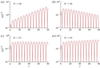
Figure 19 shows the plots of changes in  $| u (t,0,0) |\,\sqrt {t}$ obtained for several values of the parameter
 $R$ in (5.2) from
 $R = 1.30$ to
 $R = 1.40$, and Reynolds number
 $Re = 10^3$. In all cases, the amplitude of
 $|u|\,\sqrt {t}$ changes exponentially at large
 $t$, which confirms the qualitative agreement of numerical calculations with the asymptotic theory. For the largest of the presented
 $R$ values,
 $R = 1.40$, an exponential increase in
 $|u|\,\sqrt {t}$, and thus the increase in the amplitude of perturbation oscillations at the point under consideration, is observed clearly for large values of
 $t$. At
 $R = 1.30$, asymptotic decay is observed clearly. At
 $R = 1.33$ and
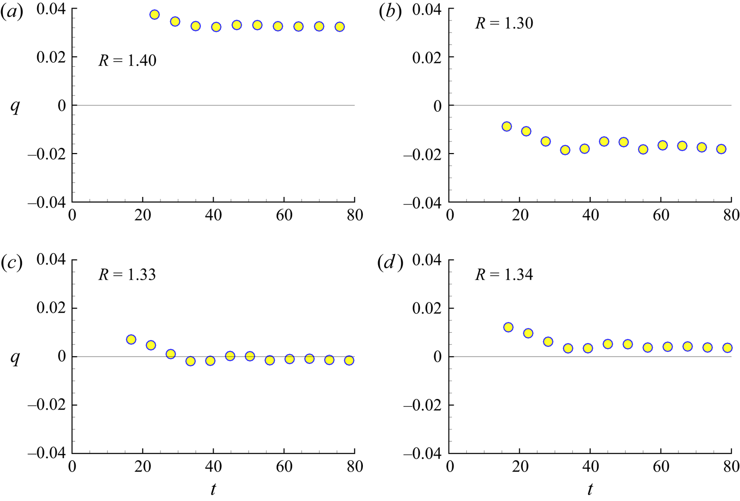
 $R = 1.34$, the asymptotic behaviour of the perturbation amplitude is less obvious; most likely, in the second case, there is weak growth, and in the first, weak damping. A clearer idea of the behaviour of the amplitude of perturbation oscillations at the point under consideration is given by the plots of the growth coefficient
 $q (t)$, determined at the moments
 $t = t_k$ at which
 $| u(t,0,0) |\,\sqrt {t}$ reaches local maxima. The growth rate at the time
 $t_k$ is defined as the rate of exponential change in the amplitude for one period of oscillation, and is calculated by the formula
 \begin{equation} q(t_k)= \frac{1}{t_k-t_{k-2}}\log\frac{|u(t_k,0,0)|\, \sqrt{t_k}}{|u(t_{k-2},0,0)|\,\sqrt{t_{k-2}}}.\end{equation}
Positive values of  $q$ correspond to an increase in the perturbation, and negative ones to attenuation. The
 $q(t_k)$ plots for the cases considered in figure 19 are shown in figure 20. The behaviour of
 $q (t)$ in the presented cases confirms the conclusions drawn from the analysis of the fluctuations in
 $| u(t,0,0) |\,\sqrt {t}$ shown in figure 19. For the largest and smallest values of the parameter
 $R$, the growth coefficient reaches asymptotic positive and negative values, respectively. On going from
 $R = 1.33$ to
 $R = 1.34$, the growth coefficient changes sign from negative to positive, although the fact of reaching asymptotic behaviour in these cases is less obvious.
Evolution of  $| u(t,0,0) |\,\sqrt {t}$ for several values of the parameter
 $R$ in (5.2), for
 $Re=10^3$.


To obtain a more definite conclusion, it is necessary to monitor the behaviour of the perturbation at a selected control point at larger times. However, the situation is complicated by the fact that for  $t> 80$, the maximum perturbation amplitude
 $A_{max}$ exceeds
 $10^{15}\,| u(t,0,0) |$, so when using double precision (real*8) for the representation of real numbers, the value
 $| u(t,0,0) | / A_{max}$ becomes less than the round-off error, and further monitoring of
 $| u(t,0,0) |$ becomes impossible. Thus the time interval of observation is limited by
 $t<80$, which is not always sufficient to determine the nature of the asymptotic behaviour of the perturbation at the control point as
 $t \to \infty$. To solve this problem in doubtful cases, calculations were carried out using an increased, quadruple precision (real*16) representation of real numbers, which allows more than doubling the duration of the observation time interval. In these calculations, the length of the computational domain was doubled (
 $X_m = 100$) with a proportional increase in the number of grid nodes in the
 $x$-direction.
The plots of  $q (t)$ obtained with
 $R = 1.33, 1.34$, calculated with increased accuracy of the representation of real numbers, are shown in figure 21. The growth coefficient is definitely negative at
 $R = 1.33$ and definitely positive at
 $R = 1.34$, which was unclear in figure 20. Based on the linear approximation of the limit values of
 $q(R)$ at
 $R=1.33$ and
 $1.34$, we obtain
 $R_{cr}=1.333$ for the critical value of the occurrence of absolute instability at
 $Re = 10^3$, which is close to the estimate
 $R_{cr} \approx 1.34$ made on the basis of an analysis of the perturbation evolution in the flow with symmetric velocity profile.
Growth coefficient  $q(t_k)$ (5.6) at (a)
 $R = 1.33$ and (b)
 $R = 1.34$, calculated with increased precision (real*16) of the representation of real numbers, for
 $Re=10^3$.

The obtained value of  $R_{cr}$ at the Reynolds number
 $Re = 10^3$ slightly exceeds the theoretical value
 $R_{cr} = 1.315$ obtained by Huerre & Monkewitz (Reference Huerre and Monkewitz1985) and Shikina (Reference Shikina1987) within the framework of the inviscid theory. Figure 22 shows the results of calculations performed at a larger value of the Reynolds number,
 $Re=10^4$. As expected, the critical value of the parameter
 $R$, at which the convective character of the instability changes to the absolute one, decreases with increasing
 $Re$. For
 $Re = 10^4$, the perturbation growth coefficient
 $q(t)$ at large times has a definitely negative value for
 $R = 1.31$ (figure 22a), but a positive value for
 $R = 1.32$ (figure 22b). That is, the critical value for this Reynolds number is close to
 $1.315$, which is in good agreement with the result of the inviscid theory,
 $R_{cr} = 1.315$.
Growth coefficient  $q(t_k)$ (5.6) at (a)
 $R = 1.31$ and (b)
 $R = 1.32$, calculated with increased precision (real*16) of the representation of real numbers, for
 $Re=10^4$.

5.4. Development of an impulse perturbation in a flow with a jet velocity profile
The onset of absolute instability in a shear layer flow requires both positive and negative velocities of the main flow. In this regard, the results of Lesshafft & Marquet (Reference Lesshafft and Marquet2010), Balestra et al. (Reference Balestra, Gloor and Kleiser2015) and Vedeneev & Zayko (Reference Vedeneev and Zayko2018), where the occurrence of absolute instability in the unidirectional jet flow is predicted, look interesting. Absolute instability may arise in the case when the inflection point in the velocity profile is close to the flow periphery, but the velocity gradient at this point is large enough. In this subsection, we check this possibility numerically for a jet velocity profile shown to be absolutely unstable in § 4.
The investigated jet velocity profile is shown in figure 23 and corresponds to parameters  $\xi =0.25$,
 $\zeta =2.0$. It is characterized by the presence of a wide flat area in the centre and two symmetrical areas of velocity drop at the periphery. The inflection points are located at distance
 $\pm 0.75$ from the axis of symmetry. The velocity value at these points is
 $U =0.25$.
(a) Velocity profile  $U (y)$, and (b) vorticity profile
 $-\textrm {d}U/{\textrm {d} y}$.

In accordance with the conclusions of § 3, the absolute instability of the considered jet flow can arise only with respect to perturbations, the  $y$-component of the velocity of which is antisymmetric with respect to
 $y = 0$. Therefore, just as in the shear layer flow, the initial perturbation was specified in the form (5.3), which provides the required symmetry.
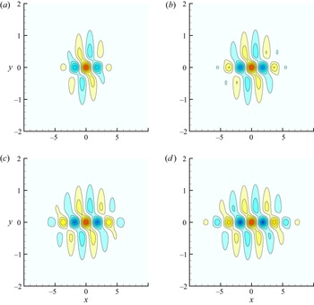
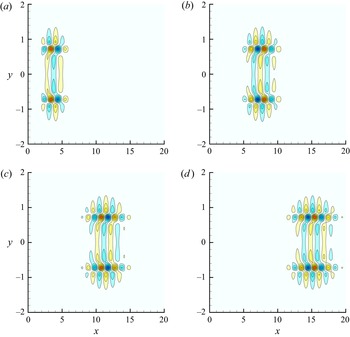
The distributions of  $u(t, x, y)$ at several successive times, obtained for
 $Re = 1000$, are shown in figure 24. Figure 25 shows the distributions of
 $| u (t, x, y_c) | / A_{max}$ along the line
 $y = y_c = 0.75$, at which the maximum shear of the main flow velocity is achieved. The evolution of the perturbation at the initial stage leads to the formation of two wave packets located symmetrically from the axis of symmetry
 $y = 0$. Each of the packets develops similarly to the development of a perturbation in the shear layer. Their characteristic size in the longitudinal direction increases with time, while in the transverse direction it remains constant. The maximum perturbation amplitude
 $A_{max}$ grows exponentially with the rate
 ${\sim } \exp (0.613t)$, and is reached at distance approximately
 $y = \pm 0.7$, which is somewhat closer to the symmetry line than the location of the inflection points in the velocity profile. Perturbations are carried away by the flow at the velocity of the main flow at these points,
 $c_f = U (\pm 0.7) \approx 0.4$.
Distributions of the  $x$-component of the perturbation velocity
 $u(t,x,y) / A_{max}(t)$ at different times: (a)
 $t=10$, (b)
 $t=20$, (c)
 $t=30$, (d)
 $t=40$, for
 $Re=1000$.

Distributions  $| u(t, x, y_c) | / A_{max}(t)$,
 $y_c = 0.75$ at different times: (a)
 $t=10$, (b)
 $t=20$, (c)
 $t=30$, (d)
 $t=40$, for
 $Re=1000$.

To determine the nature of the emerging instability, the perturbation oscillations were monitored at the control point  $(x, y) = (0, y_c = 0.75)$ at different values of the Reynolds number. The growth rate of perturbations in the jet flow is noticeably higher than in the shear layer flow considered above: for
 $Re = 1000$, the maximum amplitude increases in the jet as
 $\exp (0.613t)$, while in the shear layer the rate is
 $\exp (0.341t)$. As a result, when performing calculations with double precision of the representation of real numbers, the amplitude of the perturbation at the control point turns out to be below the level of round-off errors already starting from
 $t = 50$. This interval of observation is usually insufficient to establish the asymptotic behaviour of the perturbation. Therefore, all calculations were carried out with an increased quadruple precision of the representation of real numbers (real*16). In this case, the duration of the observation period is doubled, up to
 $t = 100$. As in the case of the shear layer, the calculations were carried out in a computational domain with size
 $200 \times 12$ (
 $X_m = 100$,
 $Y_m = 6$) on a grid with size
 $4096 \times 128$.
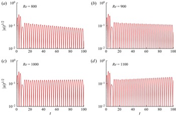
Figure 26 shows the oscillations of  $| u(t, 0, y_c) |\,\sqrt {t}$ for several values of the Reynolds number from
 $Re = 800$ to
 $Re = 1100$. For the two smallest
 $Re$ values, the amplitude of the perturbation at the control point decreases, while for the two largest, a weak increase is observed. In figure 27, the results of the same calculations are presented in the form of plots of the perturbation growth rate
 $q(t_k)$ in (5.6). The graphs in figure 27 show that the evolution of perturbations at large
 $t$ is close to asymptotic behaviour. The closest to the critical value is
 $Re=1000$. Interpolation of the limit values of
 $q(Re)$ gives an estimate
 $Re_{cr}=974$ for the critical value of the Reynolds number, at which there is a transition from convective to absolute type of instability in the flow under consideration. This estimate differs by only 1.5 % from the theoretical value
 $Re_{cr}=960$ obtained in § 4 through the saddle-point analysis (figure 13b).
Evolution of  $| u(t, 0, y_c) |\,\sqrt {t}$ in the jet flow for several values of the Reynolds number.

Growth coefficient  $q (t_k)$ in (5.6) in the jet flow at several values of the Reynolds number.

In general, the results obtained on the behaviour of the perturbation at a fixed point in space give a positive answer to the fundamental question of the possibility of the occurrence of absolute instability in a jet flow with a unidirectional velocity, which confirms the conclusions of Lesshafft & Marquet (Reference Lesshafft and Marquet2010), Balestra et al. (Reference Balestra, Gloor and Kleiser2015) and Vedeneev & Zayko (Reference Vedeneev and Zayko2018) for round jets.
6. Conclusions
In this study, we considered a two-parameter family of plane jet velocity profiles (which includes a close-to-classical jet) and showed, by saddle-point analysis, that unconfined plane jets of inviscid incompressible fluid can be absolutely unstable without the presence of counter-flow. Such jets have specific properties of velocity distribution, similar to round jets studied by Lesshafft & Marquet (Reference Lesshafft and Marquet2010), Balestra et al. (Reference Balestra, Gloor and Kleiser2015) and Vedeneev & Zayko (Reference Vedeneev and Zayko2018). Namely, at the inflection point, the velocity should be sufficiently small, and the velocity gradient sufficiently large. The first feature guarantees a small phase speed of the growing mode, and the second feature guarantees a large growth rate; both properties provide favourable conditions for coupling between growing downstream-travelling mode and damped upstream-travelling mode that results in absolute instability.
Next, we performed viscous analysis and determined critical Reynolds number values, below which the jet flow, being absolutely unstable in inviscid formulation, becomes convectively unstable. Lowering the inflection point location and a mild thinning of the shear layer yields  $Re_{cr}$ less than 500, which is quite a small value that can be achieved in experiments and analysed in direct numerical simulation. However, excessive thinning of the shear layer results in rapid growth of
 $Re_{cr}$ due to stronger effects of viscosity, which tends to damp the growing mode and to prevent its coupling with the upstream-travelling mode.
To confirm the results of the theoretical analysis, numerical simulations of the development of small impulse localized perturbations in the shear layer and jet flow were carried out. It is shown that after a short period of development, the perturbation takes the form of a wave packet localized in space, carried by the main flow at a constant velocity. The amplitude of the perturbation in the packet grows exponentially, and its size in the direction of the flow increases linearly with time. Thus the type of instability (convective/absolute) is determined by the ratio of two velocities: the rate of drift of the perturbation, and the rate of expansion of the region occupied by the perturbation. The rapid growth of the perturbation amplitude limits the possible observation time for the evolution of the perturbation at a fixed point; therefore it is difficult to determine accurately the critical parameters at which the convective instability in the considered flows is replaced by the absolute one. Nevertheless, using calculations with quadruple precision, an estimate was obtained for the condition of occurrence of absolute instability in the shear layer, which coincides with good accuracy with the theoretical results obtained in Huerre & Monkewitz (Reference Huerre and Monkewitz1985) and Shikina (Reference Shikina1987). It is shown that the nature of the instability of the jet flow constructed in § 4 of the present work changes from convective to absolute as the Reynolds number increases. An estimate of the critical Reynolds number  $Re_{cr} = 974$ is obtained, which is in excellent agreement with the theoretical result
 $Re_{cr} = 960$ obtained in § 4.
A question may arise on how jets with non-classical velocity profiles, with shifted inflection point and thinned shear layer, can be produced. For round jets, co-flowing (Hallberg et al. Reference Hallberg, Srinivasan, Gorse and Strykowski2007) or counter-flowing (Strykowski et al. Reference Strykowski, Krothapalli and Jendoubi1996) streams can be used for this purpose. Although such facilities were used for light jets, they can also be employed for the jets of constant density. Another example of apparatus is demonstrated by Zayko et al. (Reference Zayko, Teplovodskii, Chicherina, Vedeneev and Reshmin2018) and Gareev et al. (Reference Gareev, Zayko, Chicherina, Trifonov, Reshmin and Vedeneev2022): a rapidly expanding diffuser covered by a metal grid. A similar method can be used for producing plane jets. Preliminary experiments with plane jets performed by our group demonstrate that the shape of the diffuser wall effectively drives the velocity profile and, in particular, the position, velocity and gradient in the inflection point.
It is expected that organization of absolutely unstable jets can be useful in numerous technologies that employ turbulent jets. As a rule, transition to turbulence does not occur immediately, and a laminar portion, typically of the order of one diameter in length, is present even for very large Reynolds number values due to the convective nature of the instability. In the case of an absolutely unstable jet, the back edge of growing perturbations travels upstream and occupies all the jet length, yielding either secondary transient flow, or turbulization of the jet starting immediately from the orifice. Also, experimental studies of absolutely unstable hot jets (Monkewitz et al. Reference Monkewitz, Bechert, Barsikow and Lehmann1990; Hallberg et al. Reference Hallberg, Srinivasan, Gorse and Strykowski2007; Li & Juniper Reference Li and Juniper2013) demonstrate that the structure of the resulting turbulent jets is complemented, compared to ‘regular’ turbulent jets, by strong side jets and global oscillations of the flow that enhance entrainment of surrounding fluid and, consequently, mixing and heat exchange. Thus we expect that the use of absolutely unstable jets can drastically improve turbulent mixing.
Declaration of interests
The authors report no conflict of interest.
Funding
This work is supported by the Russian Science Foundation under grant 20-19-00404.
Appendix A. Explicit formulas for velocity profiles
Velocity profiles approximating a classical shear layer and those with shifted inflection point location ( $\xi \le 0.5$,
 $\zeta =1$) are given by (2.15) with the following relations:
 \begin{equation} \left.\begin{array}{c@{}} f(y)=a_5 y^5+a_4 y^4+a_3 y^3+1,\\ g(y)=b_5 (y-1)^5+b_4 (y-1)^4+b_3 (y-1)^3,\\ \end{array}\right\} \end{equation}
where  $a_j$ and
 $b_j$ are the solutions of the linear systems of equations
 \begin{gather} \left.\begin{array}{c@{}} a_5 y_0^5+a_4 y_0^4+a_3 y_0^3=\xi-1,\\ 5a_5 y_0^4+4a_4 y_0^3+3a_3 y_0^2=\eta,\\ 20a_5 y_0^3+12a_4 y_0^2+6a_3 y_0=0,\\ \end{array}\right\} \end{gather}
 \begin{gather} \left.\begin{array}{c@{}} b_5 (y_0-1)^5+b_4 (y_0-1)^4+b_3 (y_0-1)^3=\xi,\\ 5b_5 (y_0-1)^4+4b_4 (y_0-1)^3+3b_3 (y_0-1)^2=\eta,\\ 20b_5 (y_0-1)^3+12b_4 (y_0-1)^2+6b_3 (y_0-1)=0,\\ \end{array}\right\} \end{gather}
with  $\eta =-2$ and
 $y_0=1-\xi$.
The thickness of the shear layer ( $\zeta \ge 1$) is changed by the transformation (3.1), in which
 \begin{equation} \left.\begin{array}{c@{}} \varphi(y)=\alpha_5 y^5+\alpha_4 y^4+\alpha_3 y^3+\nu y,\\ \psi(y)=\beta_5 (y-1)^5+\beta_4 (y-1)^4+\beta_3 (y-1)^3+\nu (y-1)+1,\\ \end{array}\right\} \end{equation}
where  $\alpha _j$ and
 $\beta _j$ are the solutions of linear systems of equations
 \begin{gather} \left.\begin{array}{c@{}} \alpha_5 y_0^5+\alpha_4 y_0^4+\alpha_3 y_0^3=y_0(1-\nu),\\ 5\alpha_5 y_0^4+4\alpha_4 y_0^3+3\alpha_3 y_0^2=\zeta-\nu,\\ 20\alpha_5 y_0^3+12\alpha_4 y_0^2+6\alpha_3 y_0=0,\\ \end{array}\right\} \end{gather}
 \begin{gather} \left.\begin{array}{c@{}} \beta_5 (y_0-1)^5+\beta_4 (y_0-1)^4+\beta_3 (y_0-1)^3=(y_0-1)(1-\nu),\\ 5\beta_5 (y_0-1)^4+4\beta_4 (y_0-1)^3+3\beta_3 (y_0-1)^2=\zeta-\nu,\\ 20\beta_5 (y_0-1)^3+12\beta_4 (y_0-1)^2+6\beta_3 (y_0-1)=0,\\ \end{array}\right\} \end{gather}
with  $\nu =1/\zeta ^2$.