1 Introduction
After more than sixty years of research, the characteristics of the acoustic sources are well established for supersonic jets, but this is not the case for subsonic jets due to limited knowledge of jet flow turbulence, as pointed out in the reviews by Tam (Reference Tam1995, Reference Tam1998). In particular, despite the development of comprehensive theories on the generation of aerodynamic noise (Lighthill Reference Lighthill1952; Crighton Reference Crighton1975), the nature of the sources has been a matter of debate for a long time. Using localization techniques, as in Chu & Kaplan (Reference Chu and Kaplan1976) and Fisher, Harper-Bourne & Glegg (Reference Fisher, Harper-Bourne and Glegg1977) for instance, the source distribution along the axial direction in subsonic jets was, however, shown to depend on the Strouhal number
 $St_{D}=fD/u_{j}$
, where
 $f$
is the frequency, and
 $D$
and
 $u_{j}$
are the jet exit diameter and velocity. Overall, high-frequency sound sources are located near the nozzle exit, whereas low-frequency sources lie in the vicinity of the end of the jet potential core. The sound spectra measured in the acoustic field were also found to be dominated by low-frequency components in the downstream direction, but to be broadband in the sideline and upstream directions; see the far-field measurements of Mollo-Christensen, Kolpin & Martucelli (Reference Mollo-Christensen, Kolpin and Martucelli1964) for example. These observations, and other experimental and numerical findings reported in Tam (Reference Tam1998), Panda, Seasholtz & Elam (Reference Panda, Seasholtz and Elam2005) and Tam et al. (Reference Tam, Viswanathan, Ahuja and Panda2008), and in Bogey, Bailly & Juvé (Reference Bogey, Bailly and Juvé2003) and Bogey & Bailly (Reference Bogey and Bailly2006, Reference Bogey and Bailly2007), among others, suggested the presence of two noise components, namely a low-frequency component dominating in the downstream direction, marked by intermittent aspects (Juvé, Sunyach & Comte-Bellot Reference Juvé, Sunyach and Comte-Bellot1980), and a broadband component with a relatively uniform directivity. Thanks notably to the semi-empirical model of Tam & Auriault (Reference Tam and Auriault1999), the broadband component was identified as the noise of the fine-scale turbulence of the jet flow. The low-frequency component, emerging typically around
 $St_{D}=0.2$
, was attributed to the flow large-scale structures and/or instability waves. Unfortunately, despite the efforts of many researchers, its generation mechanism is still not clearly understood.
Some properties of the source radiating the downstream jet noise component have been inferred from experimental and numerical data. It appears to be located in the vicinity of the end of the potential core, where the mixing layers merge. This contention is supported by the source distributions obtained using localization techniques (Chu & Kaplan Reference Chu and Kaplan1976; Fisher et al. Reference Fisher, Harper-Bourne and Glegg1977), but also by cross-correlations calculated between flow quantities inside the jets and sound pressure outside (Seiner Reference Seiner1974; Schaffar Reference Schaffar1979; Panda et al. Reference Panda, Seasholtz and Elam2005; Bogey & Bailly Reference Bogey and Bailly2007; Panda Reference Panda2007; Grizzi & Camussi Reference Grizzi and Camussi2012). Indeed, significant values of correlations are found between the flow on the jet axis near the end of the potential core and the acoustic waves emitted at small angles relative to the downstream direction. The corresponding noise generation mechanism seems also to be related to the fact that at the end of the potential core, shear-layer turbulent structures intrude intermittently and quasi-periodically into the jet (Bogey et al. Reference Bogey, Bailly and Juvé2003). This bursting-like event was described in Tinney, Ukeiley & Glauser (Reference Tinney, Ukeiley and Glauser2008) as a volcano-like eruption forcing a highly coherent mass of fluid through the centre of the jet. It was moreover noted to occur for only a small fraction of the time but for a very high level of turbulent energy, with a regularity matching with the jet’s peak Strouhal number.
For a long time (Mollo-Christensen Reference Mollo-Christensen1967), jet noise sources have also been associated with the streamwise evolution of instability waves, which can be used to describe the dynamics of the flow coherent structures. The modelling of such waves in theoretical studies, e.g. by Kempton & Ffowcs Williams (Reference Kempton and Ffowcs Williams1978) and Tam & Morris (Reference Tam and Morris1980), just to mention a few well-known pioneers in that field, provided features consistent with jet far-field experimental data. In Crighton & Huerre (Reference Crighton and Huerre1990), in particular, it offered an explanation for the superdirective character of jet noise. Due to the spreading of the jet flow, the instability waves grow, saturate and decay, which results in a small fraction of flow components with supersonic phase velocity, radiating noise downstream, as illustrated in Tam et al. (Reference Tam, Viswanathan, Ahuja and Panda2008), Suzuki (Reference Suzuki2010) and Jordan & Colonius (Reference Jordan and Colonius2013). Nevertheless, this phenomenon alone appears to underestimate the actual sound pressure levels of jets, indicating that other important characteristics observed during the collapse of coherent structures at the end of the potential core, such as intermittency and nonlinearity, must be included in the model to increase the radiated noise levels (Cavalieri et al. Reference Cavalieri, Jordan, Agarwal and Gervais2011; Suzuki Reference Suzuki2013). For that purpose, Kastner et al. (Reference Kastner, Samimy, Hileman and Freund2006) notably proposed to use a truncated wave packet instead of a symmetric wave packet to mimic the rapid breakdown of the flow large-scale structures in the model.
In order to isolate the source of the downstream jet noise component, it can be worth dealing with a reduced or simplified jet flow configuration. One possibility is to consider temporally developing flows, as in the present work. The amplification of temporally growing disturbances in a hyperbolic–tangent velocity profile was investigated by Michalke (Reference Michalke1964) using linear stability theory. Temporally developing mixing layers have been calculated in several studies, including those by Comte, Lesieur & Lamballais (Reference Comte, Lesieur and Lamballais1992), Vreman, Sandham & Luo (Reference Vreman, Sandham and Luo1996) and Freund, Lele & Moin (Reference Freund, Lele and Moin2000a ,Reference Freund, Lele and Moin b ), in order to describe the turbulent development and the compressibility effects in free shear flows. Simulations of temporal mixing layers have also allowed for studies of noise generation and propagation in such flows; refer to Fortuné, Lamballais & Gervais (Reference Fortuné, Lamballais and Gervais2004) and Kleimann & Freund (Reference Kleimann and Freund2008) for subsonic mixing layers, and to Buchta & Freund (Reference Buchta and Freund2017) for supersonic mixing layers. Unfortunately, very few computations of temporally developing jets can be found in the literature, certainly because temporal jets do not exit from a nozzle, and have a potential core of infinite length, which renders the comparisons with spatially developing jets difficult. Some have been carried out to examine the structure of the turbulence boundary of a planar jet (van Reeuwijk & Holzner Reference van Reeuwijk and Holzner2014) and to detect the presence of upstream-propagating waves in supersonic jets by Bogey & Gojon (Reference Bogey and Gojon2017), but to the best of the author’s knowledge, the question of their sound field has never been addressed before. Therefore, it is unclear whether temporal jets radiate the same acoustic components as spatially developing jets. If this is the case, original information on potential common sound sources could be gained when dealing with such flows.
In the present work, in order to provide new insight into the generation of noise in high-subsonic jet flows when the jet potential core closes, two temporally developing isothermal round jets at a Mach number of 0.9 and diameter-based Reynolds numbers of 3125 and 12 500 are considered. They are computed on a grid extending up to 120 jet radii in the axial direction by solving the compressible Navier–Stokes equations using high-order finite-difference schemes. The main statistical properties of the jet velocity and near pressure fields and velocity and pressure autocorrelations are calculated from ten runs carried out using different initial random perturbations in the jet shear layers. The first objective is to determine whether the two temporal jets generate sound waves in the same way as spatially developing subsonic jets, including the jets of Stromberg, McLaughlin & Troutt (Reference Stromberg, McLaughlin and Troutt1980), Freund (Reference Freund2001) and Bogey & Bailly (Reference Bogey and Bailly2006, Reference Bogey and Bailly2007) at low Reynolds numbers. The particular question that arises and needs to be answered here is whether, when the jet shear layers merge, low-frequency waves are emitted in the downstream direction as happens at the end of the potential core of spatial jets. If so, this will suggest that they are produced by the same noise generation mechanism, independently of the presence of a nozzle or of a potential core of finite length. The second objective is to find connections between these waves and the potential-core closing. With this aim in view, cross-correlations will be estimated between flow quantities and sound pressure outside the jet flow to track links between sources and observer. The third objective is to extract the acoustic waves resulting from the potential-core closing from the background noise, and to reveal the corresponding noise generation mechanism in the flow. For this, conditional averages of the jet near fields will be calculated using a sample synchronization with salient flow events occurring during that closing. More precisely, these events will be detected when the minimum values of axial velocity on the jet axis due to the intermittent intrusion of turbulent structures in the jet are below an arbitrary threshold value.
The paper is organized as follows. The main characteristics of the two jets and of the simulations, including initial conditions, numerical methods, grid and computational parameters, are documented in § 2. The simulation results, namely vorticity and pressure snapshots, the properties of the jet velocity and pressure fields, flow–noise cross-correlations and conditional samplings of the jet near fields are shown in § 3. Concluding remarks are given in § 4. Finally, the sound field of a temporal jet at a Reynolds number of 50 000 is presented, and the influence of flow periodicity and of the number of runs on the statistical results and the choice of the threshold value used for the conditional sampling are discussed in four appendices.
2 Parameters
2.1 Jet definition
The two jets in this work are round and isothermal, and are characterized by a Mach number of
 $M=u_{j}/c_{a}=0.9$
and Reynolds numbers of
 $Re_{D}=u_{j}D/\unicode[STIX]{x1D708}_{a}=3125$
and
 $12\,500$
, where
 $u_{j}$
and
 $D=2r_{0}$
are the jet initial centreline velocity and diameter, and
 $c_{a}$
and
 $\unicode[STIX]{x1D708}_{a}$
are the speed of sound and kinematic molecular viscosity in the ambient medium. The ambient temperature and pressure are
 $T_{a}=293~\text{K}$
and
 $p_{a}=10^{5}~\text{Pa}$
. At initial time
 $t=0$
, the hyperbolic–tangent profiles of axial velocity presented in figure 1(a) are imposed. Following the variations of
 $\unicode[STIX]{x1D6FF}_{\unicode[STIX]{x1D703}}/r_{0}$
with the Reynolds number observed in experiments for initially laminar jets, e.g. in Zaman (Reference Zaman1985), the velocity profile in the higher Reynolds number case is twice as thin. More precisely, the momentum thickness of the mixing layer is fixed at
 $\unicode[STIX]{x1D6FF}_{\unicode[STIX]{x1D703}}=0.0358r_{0}$
for
 $Re_{D}=3125$
and
 $\unicode[STIX]{x1D6FF}_{\unicode[STIX]{x1D703}}=0.0179r_{0}$
for
 $Re_{D}=12\,500$
. This leads to initial momentum Reynolds numbers of
 $Re_{\unicode[STIX]{x1D703}}=u_{j}\unicode[STIX]{x1D6FF}_{\unicode[STIX]{x1D703}}/\unicode[STIX]{x1D708}=56$
and 112, respectively. Radial and azimuthal velocities are set to zero, pressure is equal at
 $p_{a}$
and density is determined by a Crocco–Busemann relation.
Radial profiles of (a) axial velocity
 $u_{z}/u_{j}$
at
 $t=0$
for ——
 $Re_{D}=3125$
and

 $Re_{D}=12\,500$
, and (b) radial, azimuthal and axial mesh spacings ——
 $\unicode[STIX]{x0394}r/r_{0}$
, – – –
 $r\unicode[STIX]{x0394}\unicode[STIX]{x1D703}/r_{0}$
at
 $r=r_{0}$
and –
 $\cdot$
–
 $\cdot$
 $\unicode[STIX]{x0394}z/r_{0}$
.

At
 $t=0$
, velocity perturbations of low amplitude are added in the mixing layers in order to seed the laminar–turbulent transition. For this, as proposed in Bogey et al. (Reference Bogey, Bailly and Juvé2003), divergence-free Gaussian ring vortices of radius
 $r_{0}$
are imposed. These vortices have a half-width of
 $2\unicode[STIX]{x1D6FF}_{\unicode[STIX]{x1D703}}$
, and are regularly distributed in the axial direction every
 $\unicode[STIX]{x0394}z=0.025r_{0}$
, where
 $\unicode[STIX]{x0394}z$
is the axial mesh spacing. At each position, the vortex has a maximum velocity randomly fixed between
 $0$
and
 $0.01u_{j}$
, and is weighted in the azimuthal direction by the function
 $\cos (n_{\unicode[STIX]{x1D703}}\unicode[STIX]{x1D703}+\unicode[STIX]{x1D711})$
where
 $n_{\unicode[STIX]{x1D703}}$
and
 $\unicode[STIX]{x1D711}$
are randomly chosen between 0 and 32 and between 0 and
 $2\unicode[STIX]{x03C0}$
, respectively. This allows a peak root-mean-square (r.m.s.) value of velocity fluctuations of approximately
 $0.01u_{j}$
to be obtained at
 $t=0$
. Finally, note that ten runs are performed for each Reynolds number using different random seeds in order to improve the statistical convergence of the results.
The reasons for the choice of the Reynolds numbers of
 $3125$
and
 $12\,500$
are manyfold. First, it is possible to carry out very well-resolved numerical simulations of the two temporal jets on grids of large extent in the axial direction, where periodic conditions are applied and statistical averaging is performed. This is not the case for a jet at a Reynolds number of
 $50\,000$
for instance, as will be illustrated in appendix A. Second, according to experiments, jets at low Reynolds numbers, typically below
 $Re_{D}=10^{5}$
, are initially laminar (Crighton Reference Crighton1981; Zaman Reference Zaman1985). Therefore, it does not appear necessary to impose a boundary-layer profile at
 $t=0$
, which would be difficult in the present simulations because of the absence of a nozzle. Third, the downstream noise component of subsonic jets is expected to persist at low Reynolds numbers (Stromberg et al.
Reference Stromberg, McLaughlin and Troutt1980; Kastner et al.
Reference Kastner, Samimy, Hileman and Freund2006; Bogey & Bailly Reference Bogey and Bailly2007). It may even be more predominant than at high Reynolds numbers, which should help us to extract its associated generation mechanism.
2.2 Numerical methods
The numerical framework is identical to that used in recent simulations of round jets (Bogey & Bailly Reference Bogey and Bailly2010; Bogey, Marsden & Bailly Reference Bogey, Marsden and Bailly2012, Reference Bogey, Marsden and Bailly2011b
; Bogey & Marsden Reference Bogey and Marsden2016). The simulations have been carried out using an in-house solver of the three-dimensional filtered compressible Navier–Stokes equations in cylindrical coordinates
 $(r,\unicode[STIX]{x1D703},z)$
based on low-dissipation and low-dispersion, high-order explicit schemes. The axis singularity is taken into account by the method of Mohseni & Colonius (Reference Mohseni and Colonius2000). In order to alleviate the time-step restriction near the cylindrical origin, the derivatives in the azimuthal direction around the axis are calculated at coarser resolutions than permitted by the grid (Bogey, de Cacqueray & Bailly Reference Bogey, de Cacqueray and Bailly2011a
). For the points closest to the jet axis, they are evaluated using
 $16$
points, yielding an effective resolution of
 $2\unicode[STIX]{x03C0}/16$
. Fourth-order eleven-point centred finite differences are used for spatial discretization, and a second-order six-stage Runge–Kutta algorithm is implemented for time integration (Bogey & Bailly Reference Bogey and Bailly2004). A twelfth-order eleven-point centred filter is applied explicitly to the flow variables every time step in order to remove grid-to-grid oscillations while leaving larger scales mostly unaffected. Non-centred finite differences and filters are also used near the grid boundaries (Berland et al.
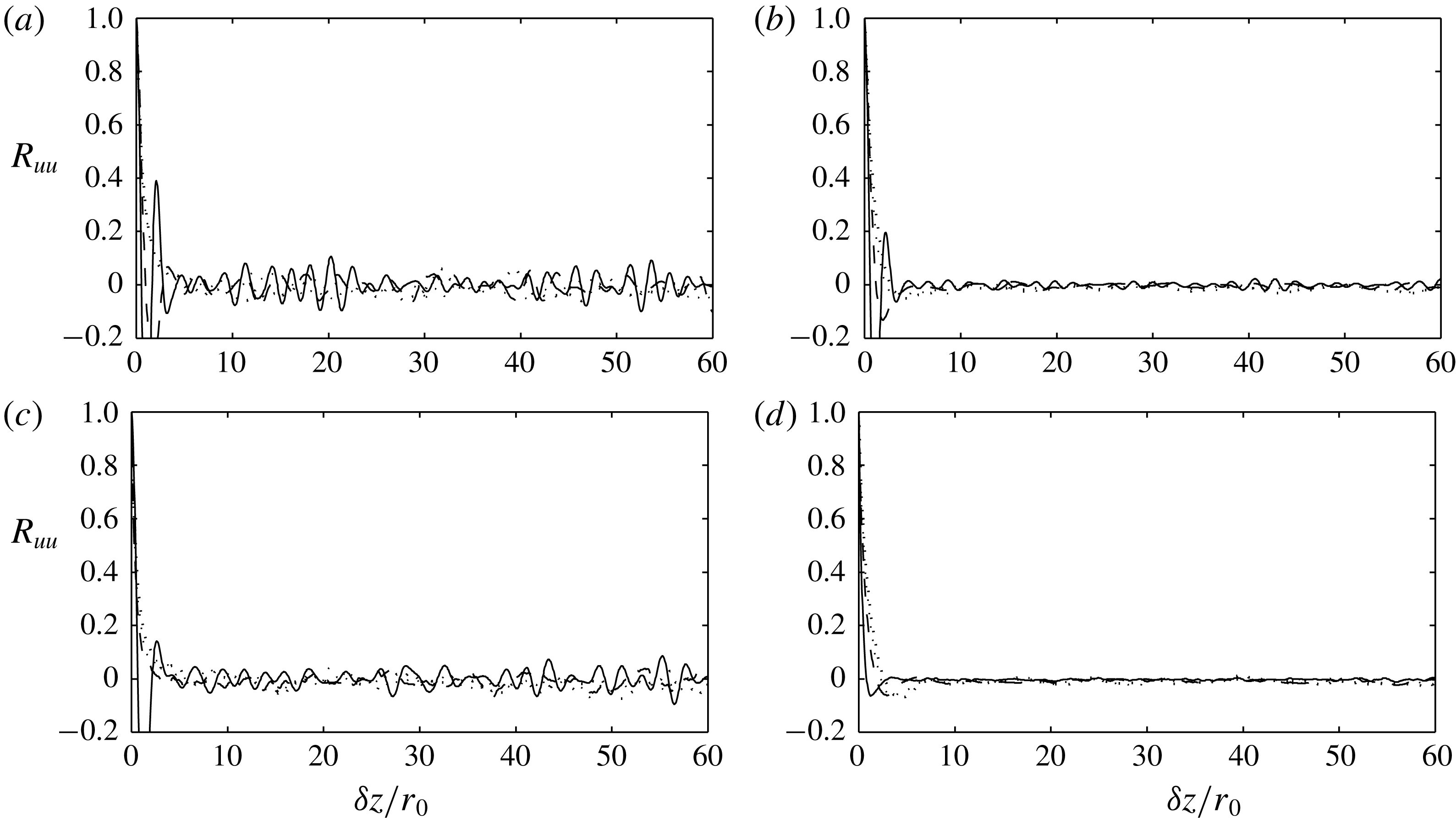
Reference Berland, Bogey, Marsden and Bailly2007; Bogey & Bailly Reference Bogey and Bailly2010). The radiation conditions of Tam & Dong (Reference Tam and Dong1996), extended to three dimensions in Bogey & Bailly (Reference Bogey and Bailly2002), are applied at the sideline boundaries to avoid significant acoustic reflections. Since a temporally developing flow is considered, periodic boundary conditions are imposed in the axial direction. Given the size of the computation domain in that direction, as shown in appendix B providing velocity correlation functions in the jets at
 $r=0$
and
 $r=r_{0}$
at different times, these conditions do not appear to distort the jet flow development.
2.3 Simulation parameters
The mesh grid used in the different runs extends up to
 $z=120r_{0}$
in the axial direction, and out to
 $r=30r_{0}$
in the radial direction. It contains
 $n_{r}\times n_{\unicode[STIX]{x1D703}}\times n_{z}=382\times 512\times 4800=940$
million points. The mesh spacing in the axial direction is uniform and equal to
 $\unicode[STIX]{x0394}z=0.025r_{0}$
, whereas, as illustrated in figure 1(b), the mesh spacing in the radial direction varies significantly. The latter is equal to a minimum value of
 $\unicode[STIX]{x0394}r=0.006r_{0}$
at
 $r=r_{0}$
, and to
 $\unicode[STIX]{x0394}r=0.025r_{0}=\unicode[STIX]{x0394}z$
on the jet axis. It is maximum and equal to
 $\unicode[STIX]{x0394}r=0.2r_{0}$
for
 $r\geqslant 16r_{0}$
, yielding a Strouhal number of
 $St_{D}=2.8$
for an acoustic wave discretized by four points per wavelength. The use of
 $n_{\unicode[STIX]{x1D703}}=512$
points in the azimuthal direction leads to the azimuthal mesh spacings of
 $r\unicode[STIX]{x0394}\unicode[STIX]{x1D703}=0.012r_{0}$
at
 $r=r_{0}$
and of
 $r\unicode[STIX]{x0394}\unicode[STIX]{x1D703}=0.025r_{0}=\unicode[STIX]{x0394}z$
at
 $r=2r_{0}$
. Furthermore, the simulations have been checked, from the calculation of the turbulent kinetic energy budgets, to be fully resolved direct numerical simulations for the jet at
 $Re_{D}=3125$
and very well-resolved large-eddy simulations for the jet at
 $Re_{D}=12\,500$
.
The computations have been performed using an OpenMP-based in-house solver on 16-core and 32-core nodes of Intel Xeon E5 processors. In order to ensure the stability of the explicit time advancement, the time step
 $\unicode[STIX]{x0394}t$
is chosen so that
 $\unicode[STIX]{x0394}t=0.6\unicode[STIX]{x0394}r(r=r_{0})/c_{a}$
for the jet at
 $Re_{D}=3125$
, and
 $\unicode[STIX]{x0394}t=\unicode[STIX]{x0394}r(r=r_{0})/c_{a}$
for
 $Re_{D}=12\,500$
. Its lowering as the Reynolds number decreases is due to the integration of the viscous fluxes. The total number of iterations is equal to 22 600 for
 $Re_{D}=3125$
and to 13 600 for
 $Re_{D}=12\,500$
, to reach a final time of
 $t=75r_{0}/u_{j}$
in both cases. During the simulations, density, the three velocity components, pressure and vorticity norm are recorded on the jet axis at
 $r=0$
and on the cylindrical surfaces at
 $r=r_{0}$
,
 $4r_{0}$
and
 $20r_{0}$
, at a sampling frequency allowing time spectra to be computed up to
 $St_{D}=10$
, and on the four azimuthal planes at
 $\unicode[STIX]{x1D703}=0$
,
 $\unicode[STIX]{x03C0}/2$
,
 $\unicode[STIX]{x03C0}$
and
 $3\unicode[STIX]{x03C0}/2$
, at half the frequency mentioned above. The statistical results obtained in each run are averaged over the periodic directions
 $z$
and
 $\unicode[STIX]{x1D703}$
. For both jets, the results of the different runs are then ensemble averaged, providing mean values, denoted by
 $\langle .\rangle$
in what follows, calculated over an equivalent distance of
 $1200r_{0}$
in the streamwise direction. Thus, the statistics can be considered to be well converged. This is demonstrated in appendix C comparing results, namely mean centreline velocities, peak turbulence intensities and r.m.s. values and spectra of pressure fluctuations, obtained from 5 and 10 runs for the two jets.
3 Results
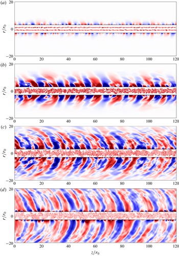
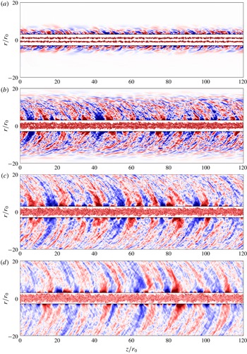
3.1 Vorticity and pressure snapshots
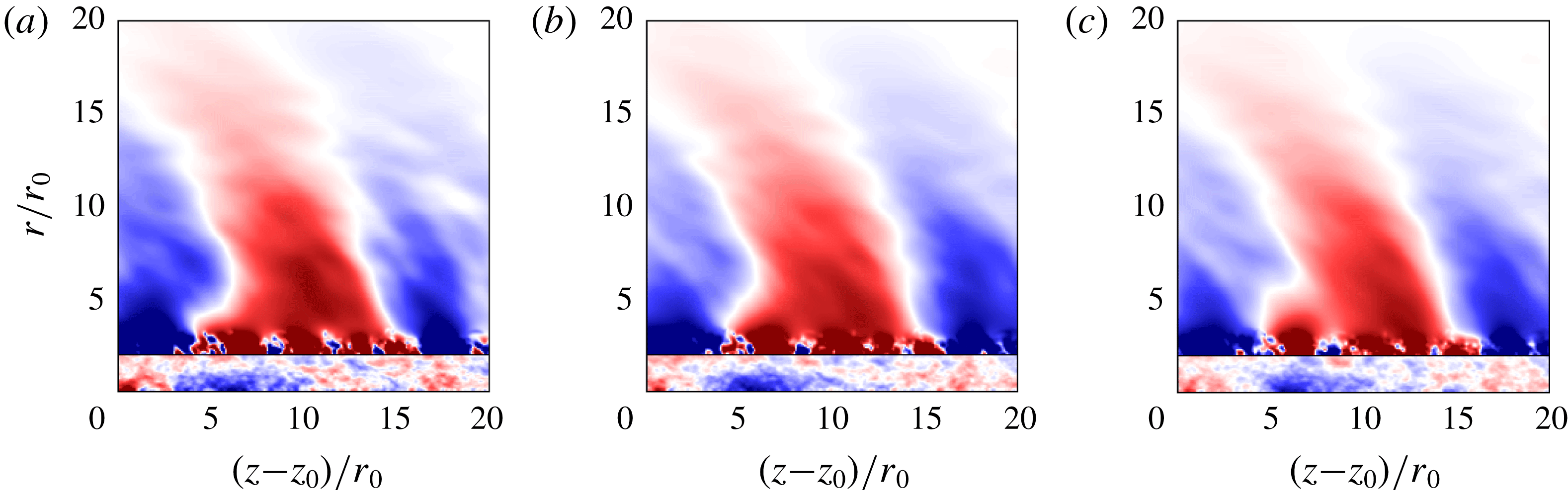
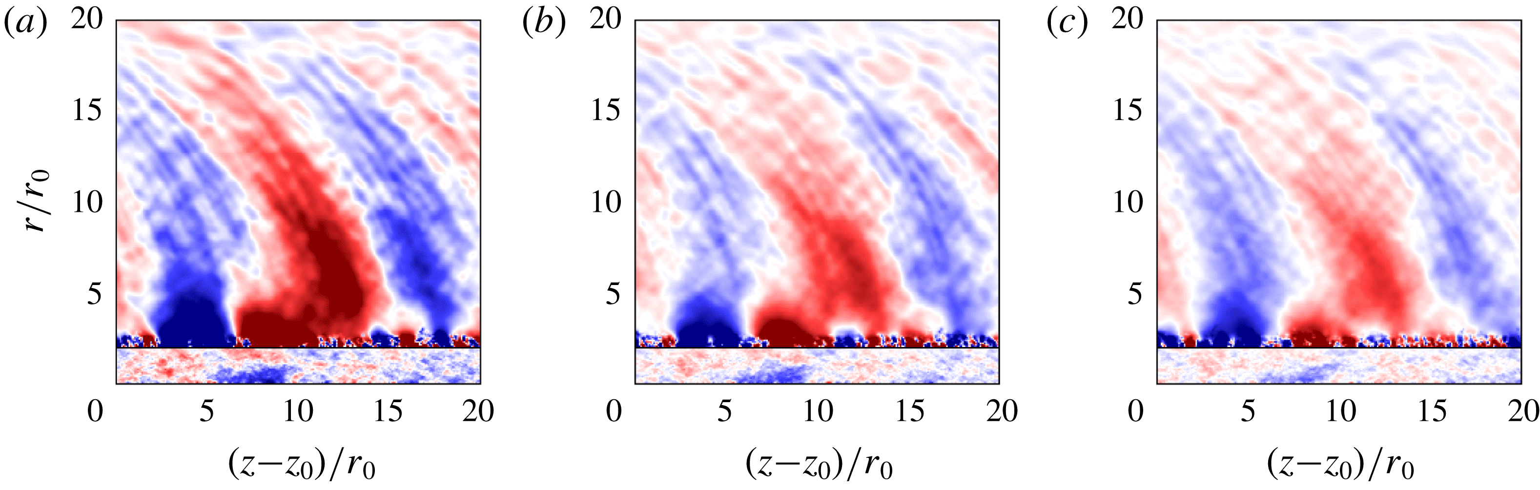
Snapshots of the vorticity norm and pressure fluctuations obtained in the
 $(z,r)$
plane for the jets at
 $Re_{D}=3125$
and
 $Re_{D}=12\,500$
are represented, respectively, in figure 2 at times
 $tu_{j}/r_{0}=15$
, 25, 35 and 45 and in figure 3 at
 $tu_{j}/r_{0}=10$
, 20, 30 and 40, and in the corresponding movies movie_fig2 and movie_fig3 available at https://doi.org/10.1017/jfm.2018.864.
Representation of vorticity norm for
 $r\leqslant 3r_{0}$
and of pressure fluctuations otherwise, obtained for
 $Re_{D}=3125$
at
 $tu_{j}/r_{0}=15$
, 25, 35 and 45, from top to bottom. The colour scales range up to the level of
 $5u_{j}/r_{0}$
for vorticity, and from
 $-250$
to
 $250~\text{Pa}$
for pressure, from blue to red.

Representation of vorticity norm for
 $r\leqslant 3r_{0}$
and of pressure fluctuations otherwise, obtained for
 $Re_{D}=12\,500$
at
 $tu_{j}/r_{0}=10$
, 20, 30 and 40, from top to bottom. The colour scales range up to the level of
 $5u_{j}/r_{0}$
for vorticity, and from
 $-200$
to
 $200~\text{Pa}$
for pressure, from blue to red.

For both Reynolds numbers, two mixing layers can be seen on both sides of the jet axis in figures 2(a) and 3(a). They have just rolled up following the growth of instability waves in the hyperbolic–tangent velocity profile (Michalke Reference Michalke1964) for
 $Re_{D}=3125$
, whereas they appear to be turbulent for
 $Re_{D}=12\,500$
. In figures 2(b) and 3(b), the mixing layers, which have developed thanks to the vortex-pairing mechanism (Winant & Browand Reference Winant and Browand1974), merge on the jet axis, resulting in the disappearance of the potential core. Finally, in figures 2(c,d) and 3(c,d), the jets are fully developed, and contain vortical scales of intensity decreasing with time. Furthermore, more fine turbulent scales are observed in the higher Reynolds number jet, as expected.
For
 $Re_{D}=3125$
, in figure 2, alternatively positive and negative fluctuations are found at
 $tu_{j}/r_{0}=15$
in the pressure field in the close vicinity of the jet. They are most likely the footprints of the coherent turbulent structures of the jet flow in the near field (Arndt, Long & Glauser Reference Arndt, Long and Glauser1997; Coiffet et al.
Reference Coiffet, Jordan, Delville, Gervais and Ricaud2005). At
 $tu_{j}/r_{0}=25$
, as the potential core closes, high-amplitude waves are emitted in the downstream direction. These waves are well visible at later times
 $tu_{j}/r_{0}=35$
and 45. They appear to be symmetric with respect to the jet centreline and to have a typical wavelength of approximately
 $15r_{0}$
. Moreover, they propagate mainly in the downstream direction, and have a very large spatial extent along the wave front direction. Interestingly, they look like the waves emitted at shallow angles by spatially developing subsonic jets at both low and high Reynolds numbers; see for instance the simulation results in Bogey & Bailly (Reference Bogey and Bailly2006) and Bogey (Reference Bogey2018).
For
 $Re_{D}=12\,500$
, in figure 3, the pressure field exhibits, unsurprisingly, more waves of short wavelength than previously for
 $Re_{D}=3125$
, but also additional noise components, whose contribution will be later quantified in the pressure spectra of figure 14. In particular, sound waves generated by vortex pairings in the mixing layers are noted at
 $tu_{j}/r_{0}=10$
and 20. In addition, upstream-propagating high-frequency waves are detected at
 $tu_{j}/r_{0}=30$
and 40 after the potential-core closing, which was not the case for the first jet. At these two times, more importantly given the aim of the present study, low-frequency waves are found to propagate in the downstream direction. Even at a lower level, they resemble those obtained for the jet at
 $Re_{D}=3125$
. Similar acoustic waves of comparable amplitude also appear to be radiated by a temporal jet at
 $Re_{D}=50\,000$
, computed in an extra simulation reported in appendix A. Therefore, these downstream-propagating sound waves, as well as their corresponding noise generation mechanism, persist when the Reynolds number increases, despite the richer spectral content of the jet turbulence, hence the relative weakening of the flow large-scale structures, in that case. Furthermore, they seem not to depend much on the shear-layer initial momentum thickness given that at
 $t=0$
, one sets
 $\unicode[STIX]{x1D6FF}_{\unicode[STIX]{x1D703}}=0.0358r_{0}$
for
 $Re_{D}=3125$
,
 $\unicode[STIX]{x1D6FF}_{\unicode[STIX]{x1D703}}=0.0179r_{0}$
for
 $Re_{D}=12\,500$
and
 $\unicode[STIX]{x1D6FF}_{\unicode[STIX]{x1D703}}=0.0089r_{0}$
for
 $Re_{D}=50\,000$
.
3.2 Properties of the velocity fields
3.2.1 Velocity field statistics
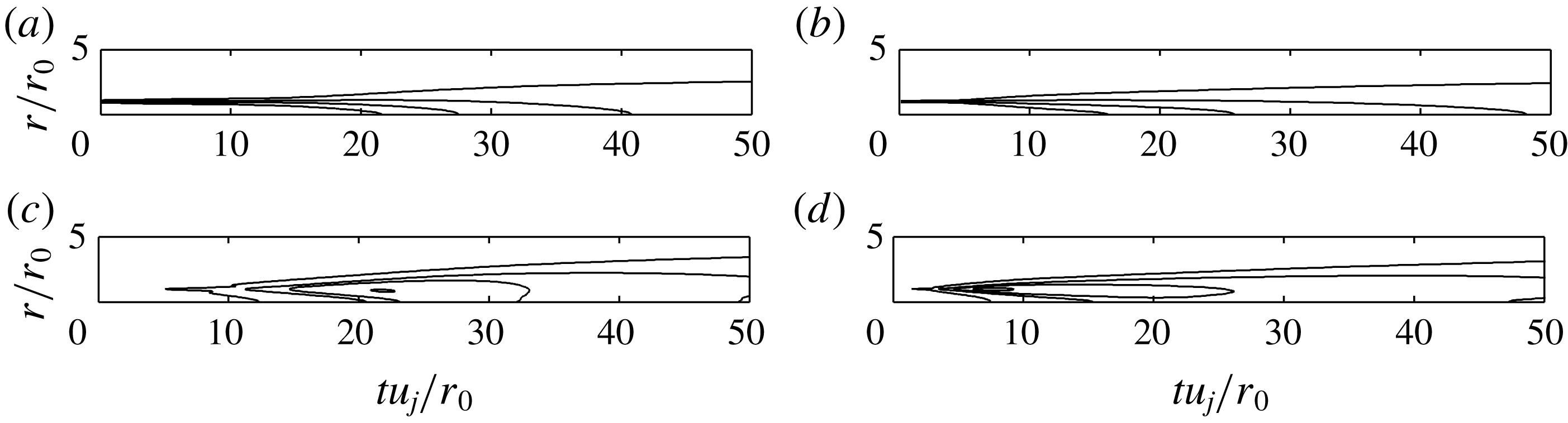
The mean and r.m.s. values of axial velocity calculated for the jets are represented in figure 4 using
 $(t,r)$
coordinates. The results bear striking similarities to the flow fields measured in the
 $(z,r)$
plane of spatially developing subsonic jets, by Zaman (Reference Zaman1986) for example. The mean axial velocity fields of figure 4(a,b) show the jet development with time, and indicates that the potential core closes at
 $tu_{j}/r_{0}\simeq 21$
for
 $Re_{D}=3135$
and earlier at
 $tu_{j}/r_{0}\simeq 16$
for
 $Re_{D}=12\,500$
. In parallel, the axial turbulence intensities are found in figure 4(c,d) to grow in the jet shear layer, to reach values slightly higher than 20 %, and then to decrease. The peak values are obtained around
 $tu_{j}/r_{0}=21$
for
 $Re_{D}=3135$
and
 $tu_{j}/r_{0}=8$
for
 $Re_{D}=12\,500$
, that is near the time of potential-core closing in the first case, but significantly before in the second case.
Space–time representation of (a,b) mean and (c,d) r.m.s. fields of axial velocity for (a,c)
 $Re_{D}=3125$
and (b,d)
 $Re_{D}=12\,500$
using the contour line values: (a,b)
 $\langle u_{z}\rangle /u_{j}=0.05$
, 0.35, 0.65 and 0.95, (c,d)
 $\langle u_{z}^{\prime }u_{z}^{\prime }\rangle ^{1/2}/u_{j}=0.02$
, 0.08, 0.14 and 0.20.

The time variations of the shear-layer momentum thickness, calculated here as
 $$\begin{eqnarray}\unicode[STIX]{x1D6FF}_{\unicode[STIX]{x1D703}}=\int _{0}^{r_{0.001}}\frac{\langle u_{z}\rangle }{\langle u_{z}\rangle (r=0)}\left(1-\frac{\langle u_{z}\rangle }{\langle u_{z}\rangle (r=0)}\right)\,\text{d}r,\end{eqnarray}$$
where
 $r_{0.001}$
is such that
 $\langle u_{z}\rangle (r=r_{0.001})=0.001\langle u_{z}\rangle (r=0)$
, and of the mean centreline axial velocity are plotted in figure 5. In figure 5(a), the shear layers appear to spread slowly when the jet flows are laminar or turbulent, but more rapidly during the laminar–turbulent transitional periods, which happen between
 $tu_{j}/r_{0}\simeq 12.5$
and
 $25$
for
 $Re_{D}=3125$
, and between
 $tu_{j}/r_{0}\simeq 5$
and
 $12.5$
for
 $Re_{D}=12\,500$
. In figure 5(b), the velocity decays after the potential-core closing starts at
 $t_{c}u_{j}/r_{0}=21.6$
for
 $Re_{D}=3125$
and at
 $t_{c}u_{j}/r_{0}=16$
for
 $Re_{D}=12\,500$
, where
 $t_{c}$
is arbitrarily defined by
 $\langle u_{z}(r=0,t=t_{c})\rangle =0.95u_{j}$
. Afterwards, the decay occurs at a higher rate in the lower Reynolds number case.
Time variations of (a) shear-layer momentum thickness
 $\unicode[STIX]{x1D6FF}_{\unicode[STIX]{x1D703}}/r_{0}$
and (b) mean axial velocity
 $\langle u_{z}\rangle /u_{j}$
at
 $r=0$
for ——
 $Re_{D}=3125$
and

 $Re_{D}=12\,500$
.

The time variations of the r.m.s. values and of the skewness factors of axial velocity fluctuations at
 $r=0$
and
 $r=r_{0}$
are displayed in figure 6. In figure 6(a), strong humps are obtained in the profiles of turbulence intensity, leading to maximum values of 17 % at
 $r=0$
and 20 % at
 $r=r_{0}$
for
 $Re_{D}=3125$
, and of 12.6 % at
 $r=0$
and 21.3 % at
 $r=r_{0}$
for
 $Re_{D}=12\,500$
. They result from the merging of vortical structures in the shear layers and on the jet centreline, respectively (Bogey & Bailly Reference Bogey and Bailly2010). As expected, due to the difference in mean flow development, they occur more rapidly in the
 $Re_{D}=12\,500$
case. Moreover, the peak value at
 $r=r_{0}$
is reached much earlier than the peak value at
 $r=0$
for
 $Re_{D}=12\,500$
, but that is not true for
 $Re_{D}=3125$
. This suggests the presence of vortex pairings in the mixing layers only in the higher Reynolds number jet.
In figure 6(b), values of skewness around
 $-1.1$
are found at
 $r=0$
close to the time of potential-core closing for both Reynolds numbers. This indicates intermittent occurrence of velocity deficits on the jet centreline at that time. These deficits follow the intrusion of shear-layer turbulent structures in the potential core of the temporal jet, as it happens at the end of the potential core of spatially developing jets (Bogey et al.
Reference Bogey, Bailly and Juvé2003; Bogey & Bailly Reference Bogey and Bailly2007). At
 $r=r_{0}$
, the results are quite different from those at
 $r=0$
. In this case, the skewness factor is slightly positive, suggesting possible bursts of high-velocity flow structures in the mixing layers.
Time variations of (a) axial turbulence intensity
 $\langle u_{z}^{\prime }u_{z}^{\prime }\rangle ^{1/2}/u_{j}$
and (b) the skewness factor of axial velocity fluctuations
 $u_{z}^{\prime }$
: at
 $r=0$
for ——
 $Re_{D}=3125$
and

 $Re_{D}=12\,500$
, and at
 $r=r_{0}$
for – – –
 $Re_{D}=3125$
and

 $Re_{D}=12\,500$
.

3.2.2 Velocity spectra
Spectra of axial velocity fluctuations computed in the jet flows at
 $r=0$
and
 $r=r_{0}$
are represented in figure 7 as a function of normalized axial wavenumber
 $k_{z}r_{0}$
, up to the value of
 $k_{z}r_{0}=60$
which is close to the filtering cutoff wavenumber of
 $k_{z}r_{0}=62.8$
obtained for four points per wavelength. The spectra calculated on the jet axis at the times of peak turbulence intensity level
 $tu_{j}/r_{0}=26.2$
for
 $Re_{D}=3125$
and
 $tu_{j}/r_{0}=22.8$
for
 $Re_{D}=12\,500$
, just after the potential-core closing, are depicted in figure 7(a). They have similar shapes and are consistent with the
 $k_{z}^{-5/3}$
power law for
 $k_{z}r_{0}\geqslant 2$
. However, the spectrum for
 $Re_{D}=3125$
contains stronger low-frequency components than that for
 $Re_{D}=12\,500$
. It seems also to be dominated by components around
 $k_{z}r_{0}\simeq 0.4$
, corresponding to a wavelength of
 $\unicode[STIX]{x1D706}_{z}\simeq 15r_{0}$
, which is not the case for the higher Reynolds number jet.
The velocity spectra estimated at
 $r=r_{0}$
are shown in figure 7(b). At the early times of
 $tu_{j}/r_{0}=2$
for
 $Re_{D}=3125$
and
 $tu_{j}/r_{0}=1$
for
 $Re_{D}=12\,500$
, components are found to emerge around wavenumbers
 $k_{z}r_{0}=4.8$
and
 $10.2$
, respectively. These peak wavenumbers are slightly lower than those given by the inviscid linear stability theory of Michalke (Reference Michalke1964), predicting that the amplification of temporally growing instability waves is maximum at
 $k_{z}r_{0}=6.2$
and
 $12.4$
in the two hyperbolic–tangent velocity profiles imposed at
 $t=0$
. The discrepancy between computations and theory is likely due to the initial conditions, but also to the low Reynolds numbers of
 $Re_{\unicode[STIX]{x1D703}}=56$
and 112 in the simulated shear layers. For such values, indeed, the growth rates and the peak wavenumbers of instability waves can be expected to be reduced compared to the inviscid case, as reported in the theoretical analyses conducted by Ragab & Wu (Reference Ragab and Wu1989) for two-dimensional mixing layers and by Morris (Reference Morris1976) for axisymmetric jets.
As for the velocity spectra obtained at
 $r=r_{0}$
at the times of peak turbulence intensity level
 $tu_{j}/r_{0}=21.6$
for
 $Re_{D}=3125$
and
 $tu_{j}/r_{0}=7.3$
for
 $Re_{D}=12\,500$
, also plotted in figure 7(b), they are relatively broadband, and show no clear agreement with the
 $k_{z}^{-5/3}$
power law. In this case, the dominant components are noted around
 $k_{z}r_{0}=1$
for
 $Re_{D}=3125$
and
 $k_{z}r_{0}=2.4$
for
 $Re_{D}=12\,500$
. The difference in peak wavenumber can be explained by the fact that the maximum turbulence level is reached at the time of potential-core closing for the first jet, but much earlier, in the developing mixing layers, for the other jet.
Representation of the power spectral densities of axial velocity fluctuations
 $u_{z}^{\prime }/u_{j}$
as a function of axial wavenumber
 $k_{z}r_{0}$
: (a) at
 $r=0$
at time of peak level for ——
 $Re_{D}=3125$
and

 $Re_{D}=12\,500$
, (b) at
 $r=r_{0}$
at time of peak level for ——
 $Re_{D}=3125$
and

 $Re_{D}=12\,500$
, and at
 $tu_{j}/r_{0}=2$
for – – –
 $Re_{D}=3125$
and
 $tu_{j}/r_{0}=1$
for

 $Re_{D}=12\,500$
; –
 $\cdot$
–
 $\cdot$
 $k_{z}^{-5/3}$
slope.

In order to explore the coherence of the flow field in the azimuthal direction, the velocity spectra obtained at
 $r=r_{0}$
at the times of peak turbulence intensity level are displayed in figure 8(a) as a function of azimuthal mode
 $n_{\unicode[STIX]{x1D703}}$
. The time variations of the magnitudes of modes
 $n_{\unicode[STIX]{x1D703}}=0$
,
 $1$
and
 $2$
at
 $r=r_{0}$
are also represented in figure 8(b). For both jets, at all times, the contribution of the axisymmetric mode is dominant, closely followed by the contribution of mode
 $n_{\unicode[STIX]{x1D703}}=1$
. This is in line with the results of the literature about the amplification rates of spatially growing linear instability waves in jet flows; see for example Michalke (Reference Michalke1984) for the inviscid incompressible case and Keiderling, Kleiser & Bogey (Reference Keiderling, Kleiser and Bogey2009) for a viscous jet at a Mach number of 0.9.
Representation of the power spectral densities of axial velocity fluctuations
 $u_{z}^{\prime }/u_{j}$
obtained at
 $r=r_{0}$
: (a) at time of peak level for ——
 $Re_{D}=3125$
and

 $Re_{D}=12\,500$
as a function of azimuthal mode
 $n_{\unicode[STIX]{x1D703}}$
, (b) time variations of the magnitudes of modes ——
 $n_{\unicode[STIX]{x1D703}}=0$
, – – –
 $n_{\unicode[STIX]{x1D703}}=1$
and –
 $\cdot$
–
 $\cdot$
 $n_{\unicode[STIX]{x1D703}}=2$
for
 $Re_{D}=3125$
, and

 $n_{\unicode[STIX]{x1D703}}=0$
,

 $n_{\unicode[STIX]{x1D703}}=1$
and

 $n_{\unicode[STIX]{x1D703}}=2$
for
 $Re_{D}=12\,500$
.

3.2.3 Velocity autocorrelations
In the jet flow field, the space–time autocorrelations of axial velocity fluctuations are computed at radial position
 $r$
and time
 $t$
in the following way:
 $$\begin{eqnarray}{\mathcal{R}}_{u_{z}^{\prime }u_{z}^{\prime }}(\unicode[STIX]{x1D6FF}z,\unicode[STIX]{x1D6FF}t)=\frac{\langle u_{z}^{\prime }(r,\unicode[STIX]{x1D703},z,t)u_{z}^{\prime }(r,\unicode[STIX]{x1D703},z+\unicode[STIX]{x1D6FF}z,t+\unicode[STIX]{x1D6FF}t)\rangle }{\langle u_{z}^{\prime 2}(r,\unicode[STIX]{x1D703},z,t)\rangle ^{1/2}\langle u_{z}^{\prime 2}(r,\unicode[STIX]{x1D703},z+\unicode[STIX]{x1D6FF}z,t+\unicode[STIX]{x1D6FF}t)\rangle ^{1/2}},\end{eqnarray}$$
where
 $\unicode[STIX]{x1D6FF}z$
is the spatial separation in the axial direction and
 $\unicode[STIX]{x1D6FF}t$
is the time delay.
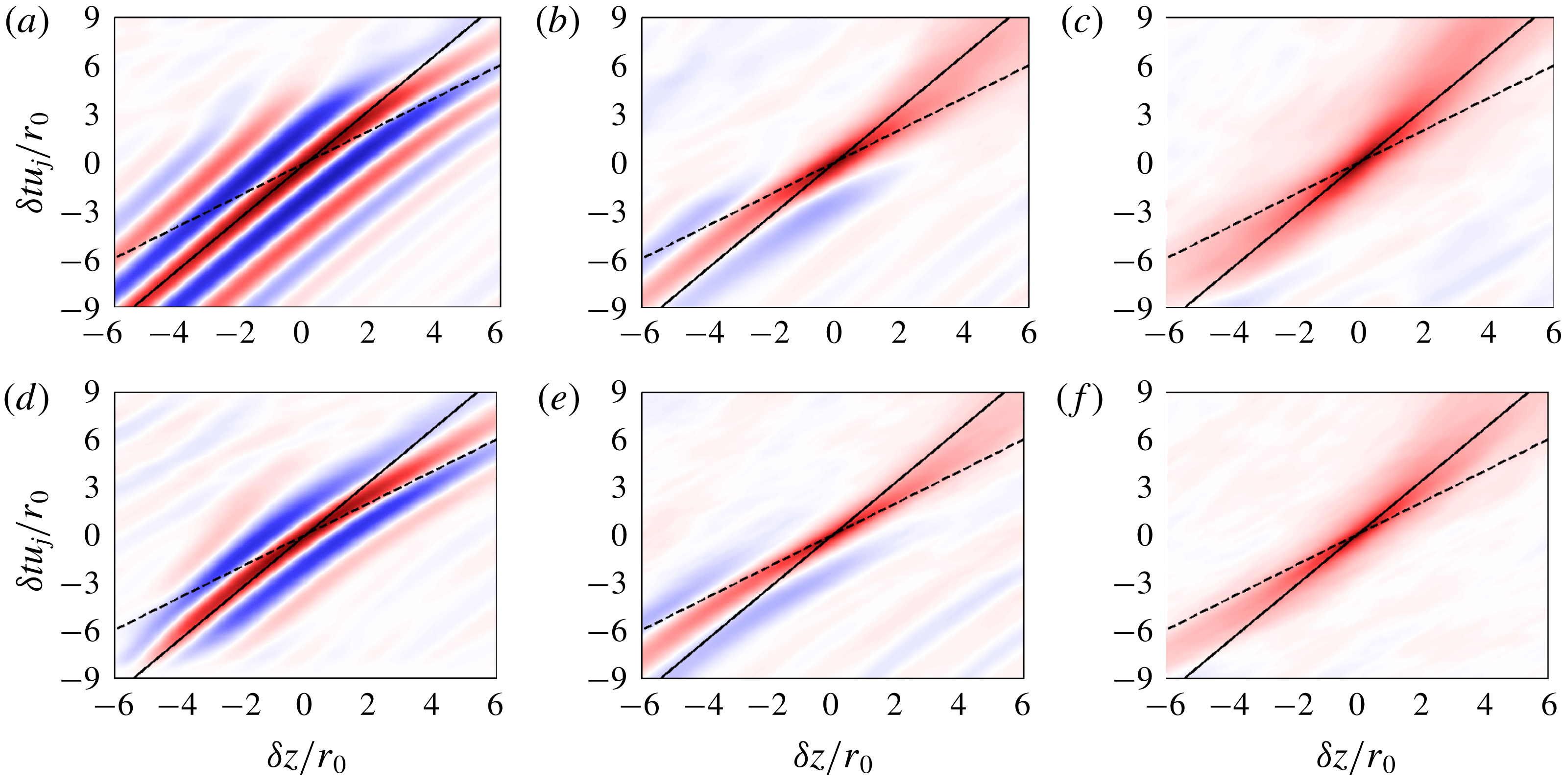
The correlation maps obtained on the jet centreline are represented in figure 9 at times
 $t=t_{c}-6r_{0}/u_{j}$
,
 $t=t_{c}$
and
 $t=t_{c}+6r_{0}/u_{j}$
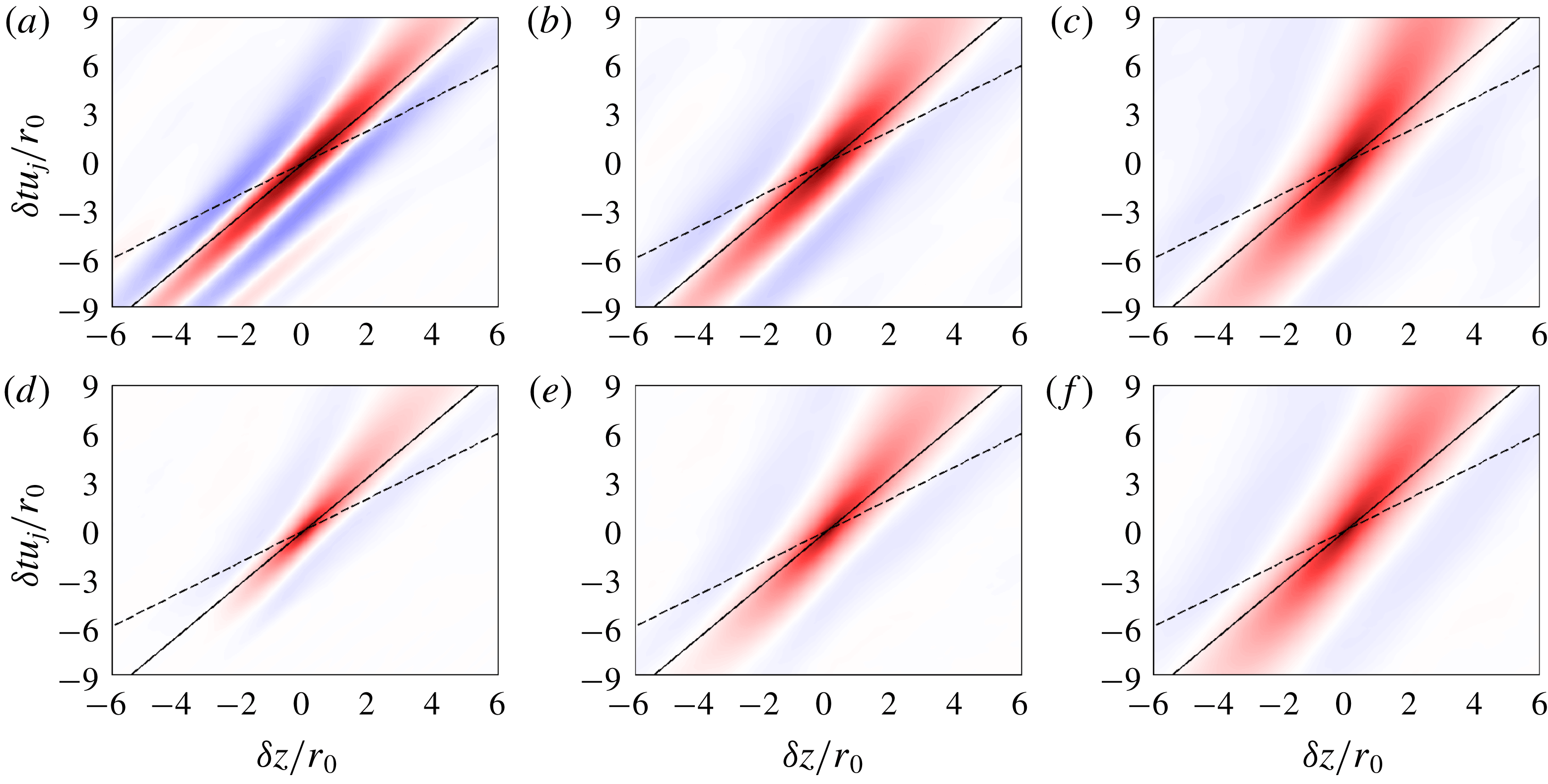
, and in the corresponding movies movie_fig9a and movie_fig9b. The solid and dashed lines show the inclinations expected for convection velocities of
 $0.6u_{j}$
and
 $u_{j}$
. The results for the two jets are similar. In figure 9(a,d), the correlations at
 $t=t_{c}-6r_{0}/u_{j}$
before the potential-core closing have an oscillating shape in the axial direction, and remain significant for very large time delays. In addition, they are well aligned with the trajectory for a convection velocity of
 $0.6u_{j}$
. In figure 9(b,e), the correlations at
 $t=t_{c}$
are comparable to the previous ones for negative time delays, but differ for positive time delays. In the latter case, the correlations are only positive and their inclination gets closer to that corresponding to a convection velocity of
 $u_{j}$
. This is due to the arrival of turbulent structures on the centreline when the potential core closes. Finally, the correlations at later times become less inclined with increasing time, as the jets develop and the velocity decays on the centreline.
Representation of the space–time correlations of axial velocity fluctuations obtained at
 $r=0$
at (a,d)
 $t=t_{c}-6r_{0}/u_{j}$
, (b,e)
 $t=t_{c}$
and (c,f)
 $t=t_{c}+6r_{0}/u_{j}$
for (a–c)
 $Re_{D}=3125$
and (d–f)
 $Re_{D}=12\,500$
; ——
 $\unicode[STIX]{x1D6FF}t=\unicode[STIX]{x1D6FF}z/(0.6u_{j})$
; – – –
 $\unicode[STIX]{x1D6FF}t=\unicode[STIX]{x1D6FF}z/u_{j}$
. The colour scale ranges from
 $-1$
to 1, from blue to red.

For comparison, the correlation maps obtained at
 $r=r_{0}$
are provided in figure 10. They resemble the correlations at
 $r=0$
given in figure 9 at the same times. Slight differences however appear. First, before the potential-core closing, significant correlation levels persist for shorter spatial separations and time delays. This may result from the fact that for
 $t<t_{c}$
, the correlations on the centreline are calculated from the footprints of the coherent structures developing in the mixing layers, whereas those at
 $r=r_{0}$
are computed from a wider variety of turbulent scales. Second, the trajectories of the correlation spots are less inclined. This is particularly true at
 $t=t_{c}$
, where they indicate a convection velocity lower than
 $0.6u_{j}$
.
Representation of the space–time correlations of axial velocity fluctuations obtained at
 $r=r_{0}$
at (a,d)
 $t=t_{c}-6r_{0}/u_{j}$
, (b,e)
 $t=t_{c}$
and (c,f)
 $t=t_{c}+6r_{0}/u_{j}$
for (a–c)
 $Re_{D}=3125$
and (d–f)
 $Re_{D}=12\,500$
; ——
 $\unicode[STIX]{x1D6FF}t=\unicode[STIX]{x1D6FF}z/(0.6u_{j})$
; – – –
 $\unicode[STIX]{x1D6FF}t=\unicode[STIX]{x1D6FF}z/u_{j}$
. The colour scale ranges from
 $-1$
to 1, from blue to red.

Some flow properties estimated from the velocity correlation functions, namely the integral length scale
 $L_{uu}^{(z)}$
and the convection velocity
 $u_{c}$
, are shown in figure 11. In figure 11(a), the integral length scales are found to increase with time. The increase occurs suddenly around the time of potential-core closing on the jet axis, but progressively at
 $r=r_{0}$
. Furthermore, at
 $t>t_{c}$
, the integral length scales are larger for
 $Re_{D}=3125$
than for
 $Re_{D}=12\,500$
, and on the jet axis than at
 $r=r_{0}$
. In figure 11(b), the convection velocities at
 $r=r_{0}$
decrease monotonically with time from
 $u_{c}\simeq 0.6u_{j}$
at
 $tu_{j}/r_{0}=10$
down to
 $u_{c}\simeq 0.3u_{j}$
at
 $tu_{j}/r_{0}=50$
. On the jet axis, on the contrary, they first increase, then reach peak values of
 $0.86u_{j}$
for
 $Re_{D}=3125$
and of
 $0.95u_{j}$
for
 $Re_{D}=12500$
near the time of potential-core closing, and finally diminish. This suggests that the turbulent structures that enter in the potential core are convected at a velocity close to the jet velocity, as in spatially developing jets (Bogey & Bailly Reference Bogey and Bailly2007).
Time variations of (a) the integral length scale
 $L_{uu}^{(z)}/r_{0}$
and (b) the convection velocity
 $u_{c}/u_{j}$
, obtained at
 $r=0$
for ——
 $Re_{D}=3125$
and

 $Re_{D}=12\,500$
, and at
 $r=r_{0}$
for – – –
 $Re_{D}=3125$
and

 $Re_{D}=12\,500$
.

3.3 Properties of the pressure fields
3.3.1 Pressure field statistics
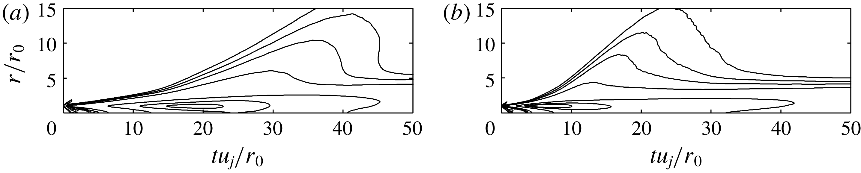
The r.m.s. values of pressure fluctuations obtained for the jets are represented in figure 12 using
 $(t,r)$
coordinates. As previously for the velocity, the results resemble the r.m.s. pressure fields acquired in the
 $(z,r)$
plane of spatially developing subsonic jets (Zaman Reference Zaman1986; Ukeiley & Ponton Reference Ukeiley and Ponton2004; Bogey et al.
Reference Bogey, Barré, Fleury, Bailly and Juvé2007). For both Reynolds numbers, the maximum values are located in the jet flows, approximately at the same position as the maximum r.m.s. values of axial velocity in figure 5(c,d). Outside the jets, lobes, whose origins seem to be the peak levels in the flow (Zaman Reference Zaman1986), are found. They reveal the production of noise in the jet and its propagation outside with increasing time. The r.m.s. pressure fields moreover suggest that the strongest acoustic waves are generated close to the time of potential-core closing for
 $Re_{D}=3125$
, but well before for
 $Re_{D}=12\,500$
, and that their main radiation angle with respect to the flow direction is larger in the latter case than in the former.
Space–time representation of the r.m.s. fields of pressure fluctuations for (a)
 $Re_{D}=3125$
and (b)
 $Re_{D}=12\,500$
using the contour line values
 $\langle p^{\prime }p^{\prime }\rangle ^{1/2}=45$
,
 $60$
, 80, 140, 1000, 3000 and 5000 Pa.

The time variations of the r.m.s. values of pressure fluctuations at
 $r=10r_{0}$
are shown in figure 13(a). The profiles reach maximum values of 83 Pa at
 $tu_{j}/r_{0}=35.4$
for
 $Re_{D}=3125$
and of 68 Pa at
 $tu_{j}/r_{0}=19$
for
 $Re_{D}=12\,500$
. Given that
 $t_{c}u_{j}/r_{0}=21.6$
in the first case and
 $t_{c}u_{j}/r_{0}=16$
in the second case, the peak for
 $Re_{D}=3125$
may be related to the potential-core closing, but it cannot be true for
 $Re_{D}=12\,500$
. In this case, it most likely results from vortex pairings in the shear layers. For completeness, the r.m.s. pressure levels obtained for
 $Re_{D}=3125$
at the three radial positions
 $r=5r_{0}$
,
 $10r_{0}$
and
 $20r_{0}$
, normalized at
 $r=10r_{0}$
using the
 $1/r$
law, are represented in figure 13(b). Peak values of 88, 83 and 85 Pa are noted at
 $tu_{j}/r_{0}=28.6$
,
 $35.4$
and
 $48$
, respectively. The similarity in amplitude supports that the spreading of the sound waves radiated by the jet is spherical. Moreover, the time delays between the peaks indicate a radiation angle of approximately 45 degrees with respect to the axial direction.
Time variations of the r.m.s. values of pressure fluctuations
 $p^{\prime }$
: (a) at
 $r=10r_{0}$
for ——
 $Re_{D}=3125$
and

 $Re_{D}=12\,500$
, (b) at ——
 $r=5r_{0}$
, – – –
 $r=10r_{0}$
and –
 $\cdot$
–
 $\cdot$
 $r=20r_{0}$
for
 $Re_{D}=3125$
normalized using a
 $1/r$
law.

3.3.2 Pressure spectra
The spectra of pressure fluctuations computed at
 $r=10r_{0}$
at
 $tu_{j}/r_{0}=35$
, 45 and 55 for
 $Re_{D}=3125$
and at
 $tu_{j}/r_{0}=30$
, 40 and 50 for
 $Re_{D}=12\,500$
are represented in figure 14 as a function of axial wavenumber
 $k_{z}r_{0}$
. At those times, the low-frequency acoustic waves generated around
 $t=t_{c}$
propagate at the radial position considered, as shown in figures 2 and 3. The three spectra for
 $Re_{D}=3125$
in figure 14(a) display very similar shapes. They contain strong components centred around a wavenumber of
 $k_{z}r_{0}\simeq 0.4$
, and decrease sharply for
 $k_{z}r_{0}>1.6$
. These components can be related to the presence of sound waves of wavelength of
 $\unicode[STIX]{x1D706}_{z}\simeq 15r_{0}$
in the pressure fields of figure 2. In the same way, the shape of the spectra for
 $Re_{D}=12\,500$
in figure 14(b) does not depend much on the time considered. With respect to the spectra for the jet at
 $Re_{D}=3125$
, they are comparable for
 $k_{z}r_{0}<1$
, but show additional high-frequency components typically between
 $k_{z}r_{0}=1.6$
and 6.4. Therefore, two contributions seem to emerge in the present sound spectra: a low-frequency contribution, noticeable at both Reynolds numbers, and a higher-frequency one, disappearing when the Reynolds number is reduced down to
 $Re_{D}=3125$
. This observation is consistent with those made based on the spectra of spatially developing jets, used as evidence for the presence of two jet noise components (Tam Reference Tam1998; Bogey & Bailly Reference Bogey and Bailly2006; Tam et al.
Reference Tam, Viswanathan, Ahuja and Panda2008). It is also supported by the comparison of the present spectra with the large-scale and fine-scale similarity spectra found empirically by Tam, Golebiowski & Seiner (Reference Tam, Golebiowski and Seiner1996) and Tam et al. (Reference Tam, Viswanathan, Ahuja and Panda2008) to fit the far-field spectra measured, respectively, in the downstream direction and in the upstream and sideline directions of both high-subsonic and supersonic jets. Indeed, the spectra for
 $Re_{D}=3125$
do not differ much from the large-scale similarity spectrum when the peak of the latter is placed at
 $(k_{z}r_{0})_{peak}=0.44$
, whereas the spectra for
 $Re_{D}=12\,500$
visibly coincide with a combination of the two similarity spectra with
 $(k_{z}r_{0})_{peak}=0.44$
and 0.55.
Representation of the power spectral densities of pressure fluctuations
 $p^{\prime }/p_{a}$
as a function of wavenumber
 $k_{z}r_{0}$
, obtained at
 $r=10r_{0}$
: (a) for
 $Re_{D}=3125$
at ——
 $tu_{j}/r_{0}=35$
, – – –
 $tu_{j}/r_{0}=45$
and –
 $\cdot$
–
 $\cdot$
 $tu_{j}/r_{0}=55$
, (b) for
 $Re_{D}=12\,500$
at ——
 $tu_{j}/r_{0}=30$
, – – –
 $tu_{j}/r_{0}=40$
and –
 $\cdot$
–
 $\cdot$
 $tu_{j}/r_{0}=50$
;


The spectra of pressure fluctuations obtained at
 $r=20r_{0}$
at
 $tu_{j}/r_{0}=45$
, 55 and 65 for
 $Re_{D}=3125$
and at
 $tu_{j}/r_{0}=40$
, 50 and 60 for
 $Re_{D}=12\,500$
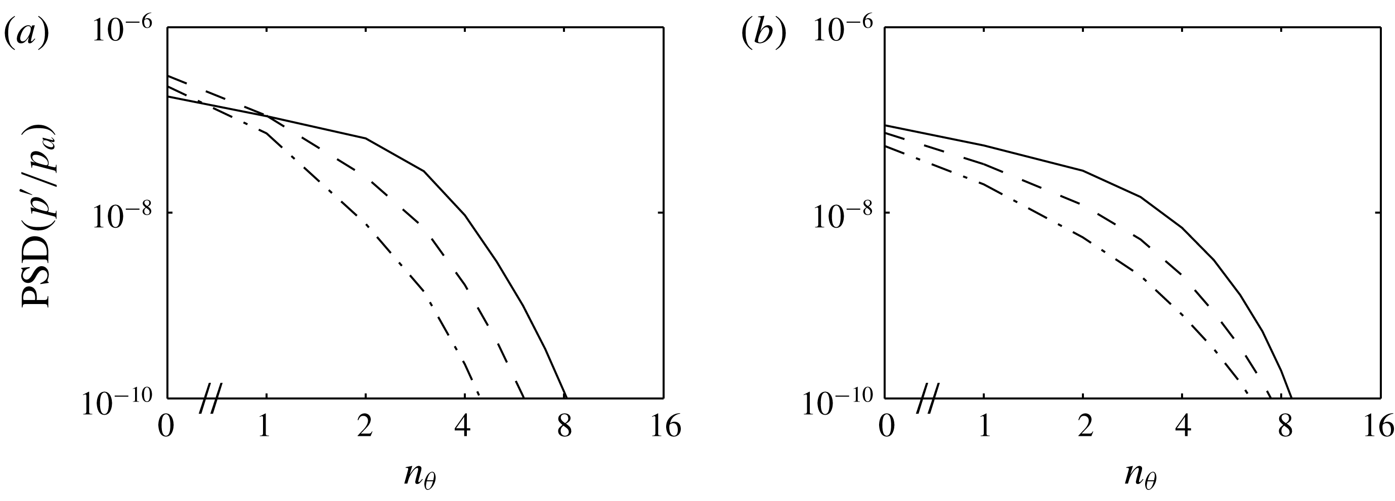
are plotted in figure 15 as a function of the azimuthal mode. In all cases, the energy is maximum for the axisymmetric mode, decreases for higher modes, and is small or negligible for modes
 $n_{\unicode[STIX]{x1D703}}>4$
. This azimuthal distribution of the acoustic pressure is close to that measured at low polar angles for spatially developing subsonic jets (Juvé, Sunyach & Comte-Bellot Reference Juvé, Sunyach and Comte-Bellot1979). For the present jets, in addition, the predominance of the axisymmetric mode is more marked as time passes, such as when lower axial angles are considered in the far field of spatial jets. That predominance is one important feature associated with the downstream subsonic jet noise component (Cavalieri et al.
Reference Cavalieri, Jordan, Colonius and Gervais2012).
Representation of the power spectral densities of pressure fluctuations
 $p^{\prime }/p_{a}$
as a function of azimuthal mode
 $n_{\unicode[STIX]{x1D703}}$
, obtained at
 $r=20r_{0}$
: (a) for
 $Re_{D}=3125$
at ——
 $tu_{j}/r_{0}=45$
, – – –
 $tu_{j}/r_{0}=55$
and –
 $\cdot$
–
 $\cdot$
 $tu_{j}/r_{0}=65$
, (b) for
 $Re_{D}=12\,500$
at ——
 $tu_{j}/r_{0}=40$
, – – –
 $tu_{j}/r_{0}=50$
and –
 $\cdot$
–
 $\cdot$
 $tu_{j}/r_{0}=60$
.

3.3.3 Pressure autocorrelations
In the jet near field, the two-dimensional spatial autocorrelations of pressure fluctuations at radial position
 $r$
and time
 $t$
are calculated as
 $$\begin{eqnarray}{\mathcal{R}}_{p^{\prime }p^{\prime }}(\unicode[STIX]{x1D6FF}r,\unicode[STIX]{x1D6FF}z)=\frac{\langle p^{\prime }(r,\unicode[STIX]{x1D703},z,t)p^{\prime }(r+\unicode[STIX]{x1D6FF}r,\unicode[STIX]{x1D703},z+\unicode[STIX]{x1D6FF}z,t)\rangle }{\langle p^{\prime 2}(r,\unicode[STIX]{x1D703},z,t)\rangle ^{1/2}\langle p^{\prime 2}(r+\unicode[STIX]{x1D6FF}r,\unicode[STIX]{x1D703},z+\unicode[STIX]{x1D6FF}z,t)\rangle ^{1/2}},\end{eqnarray}$$
where
 $\unicode[STIX]{x1D6FF}r$
and
 $\unicode[STIX]{x1D6FF}z$
are the spatial separations in the radial and axial directions.
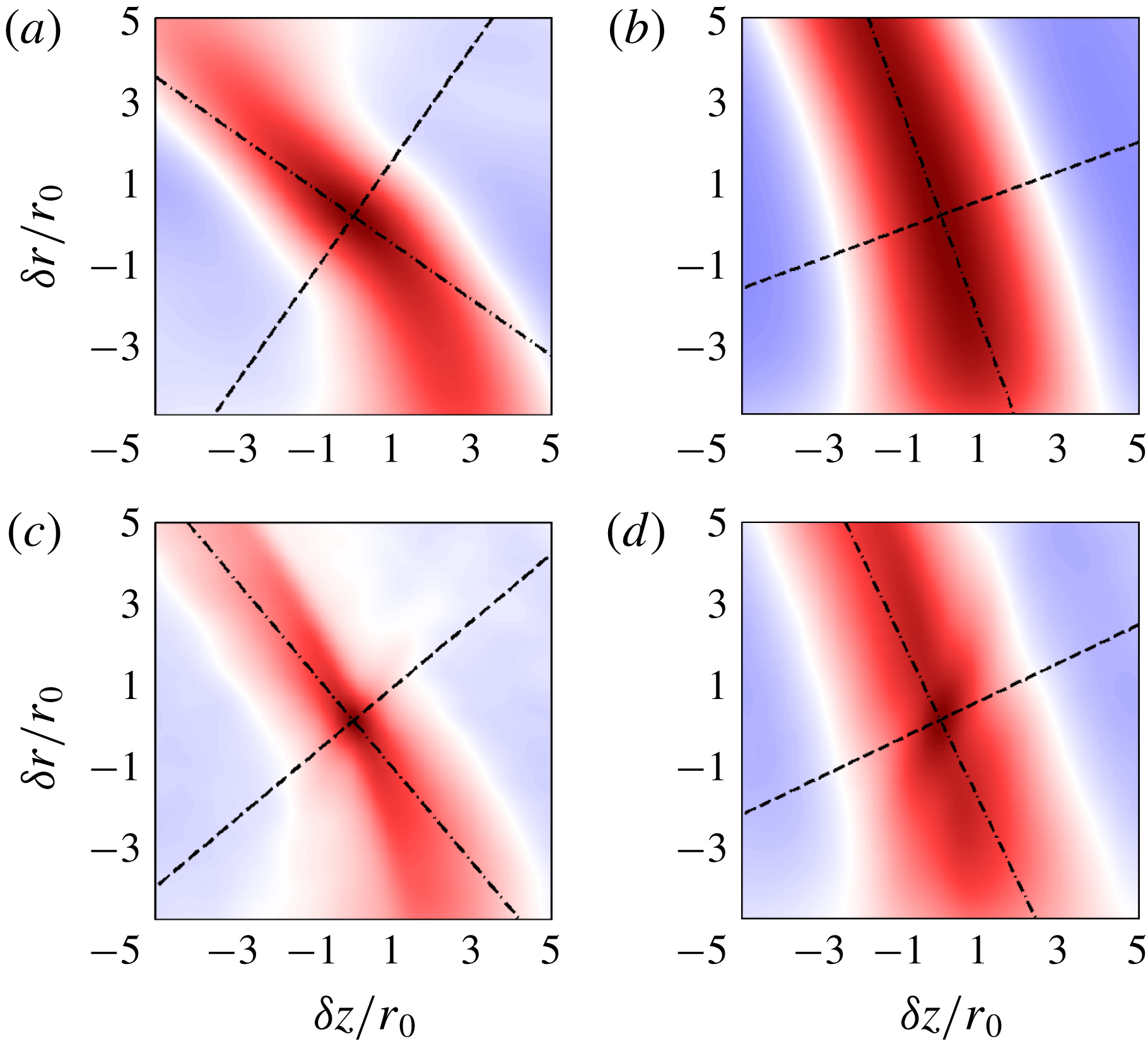
The correlation maps obtained at
 $r=10r_{0}$
at
 $tu_{j}/r_{0}=35$
and 55 for
 $Re_{D}=3125$
and at
 $tu_{j}/r_{0}=30$
and 50 for
 $Re_{D}=12\,500$
are shown in figure 16. For the two jets, the orientation of the correlation spot changes with time, indicating a direction of propagation getting closer to the jet direction. Its spatial extent also becomes larger. This is true both along the wave front, where correlation is strong over a very large distance, and normal to the wave front. For
 $Re_{D}=12\,500$
, the correlation levels are lower than for
 $Re_{D}=3125$
for large separation distances, which is consistent with the richer frequency content of the pressure spectra reported above. Furthermore, weak additional correlation spots aligned in a direction opposite to that of the main spots are visible in figure 16(c–d). They result from the acoustic waves propagating upstream in the jet near field, such as those noted in figure 3(d).
Representation of the two-dimensional spatial correlations of pressure fluctuations obtained at
 $r=10r_{0}$
for
 $Re_{D}=3125$
at (a)
 $tu_{j}/r_{0}=35$
and (b)
 $tu_{j}/r_{0}=55$
, and for
 $Re_{D}=12\,500$
at (c)
 $tu_{j}/r_{0}=30$
and (d)
 $tu_{j}/r_{0}=50$
; lines – – – aligned with and –
 $\cdot$
–
 $\cdot$
perpendicular to the average direction of acoustic propagation. The colour scale ranges from
 $-1$
to 1, from blue to red.

The radiation angles
 $\unicode[STIX]{x1D719}$
and the integral length scales
 $L_{\unicode[STIX]{x1D719}}$
computed along the average direction of propagation found from the spatial correlations of pressure at
 $r=10r_{0}$
are represented in figure 17. From
 $tu_{j}/r_{0}\simeq 30$
for
 $Re_{D}=3125$
and
 $tu_{j}/r_{0}\simeq 20$
for
 $Re_{D}=12\,500$
onwards, that is significantly after the jet potential-core closing, the radiation angles decrease with time in figure 17(a), from
 $\unicode[STIX]{x1D719}\simeq 60^{\circ }$
down to
 $\unicode[STIX]{x1D719}\simeq 30^{\circ }$
at
 $tu_{j}/r_{0}=50$
. During the same period, the integral length scales grow and reach values of approximately
 $0.9r_{0}$
at
 $tu_{j}/r_{0}=60$
. The first result is expected given that, by construction, the waves remaining at
 $r=10r_{0}$
long after their emission times can only be those propagating at low axial angles. The second one suggests an increase of the wavelength. This wavelength increase as the radiation angle decreases is consistent with the trend observed for the downstream noise component of spatial jets (Tam et al.
Reference Tam, Viswanathan, Ahuja and Panda2008). It can also be explained by a wave packet modelling of the jet noise source, as illustrated by Papamoschou (Reference Papamoschou2018), for instance.
Time variations of (a) the radiation angle
 $\unicode[STIX]{x1D719}$
and (b) the integral length scale
 $L_{\unicode[STIX]{x1D719}}/r_{0}$
along the average direction of acoustic propagation at
 $r=10r_{0}$
for ——
 $Re_{D}=3125$
and

 $Re_{D}=12\,500$
.

3.4 Flow–noise cross-correlations
In order to identify links between the flow and sound fields of the jets, it is interesting to compute cross-correlations between flow quantities and acoustic pressure, as was done in several recent experimental and numerical investigations for spatially developing jets (Seiner Reference Seiner1974; Schaffar Reference Schaffar1979; Panda et al.
Reference Panda, Seasholtz and Elam2005; Bogey & Bailly Reference Bogey and Bailly2007; Panda Reference Panda2007; Grizzi & Camussi Reference Grizzi and Camussi2012). In the present work, the axial velocity fluctuations
 $u_{z}^{\prime }$
, the product
 $u_{z}^{\prime }u_{z}^{\prime }$
and the vorticity fluctuations
 $|\unicode[STIX]{x1D714}|^{\prime }$
obtained at
 $r=0$
and
 $r=r_{0}$
, are correlated with the pressure fluctuations
 $p^{\prime }$
at
 $r=10r_{0}$
. These flow quantities are considered because they have been found in the previous studies mentioned above to correlate with far-field jet noise. Moreover, they appear in the source terms of acoustical analogies, namely
 $u_{z}^{\prime }$
and
 $u_{z}^{\prime }u_{z}^{\prime }$
in the shear-noise and self-noise source terms of Lighthill’s analogy (Ribner Reference Ribner1964), and vorticity in the vortex sound theory (Powell Reference Powell1964). The correlations are denoted by
 ${\mathcal{C}}_{u_{z}^{\prime }p^{\prime }}$
,
 ${\mathcal{C}}_{u_{z}^{\prime }u_{z}^{\prime }p^{\prime }}$
and
 ${\mathcal{C}}_{|\unicode[STIX]{x1D714}|^{\prime }p^{\prime }}$
. For
 $u_{z}^{\prime }$
, for example, they are given by
 $$\begin{eqnarray}{\mathcal{C}}_{u_{z}^{\prime }p^{\prime }}(\unicode[STIX]{x1D6FF}z,t_{1})=\frac{\langle u_{z}^{\prime }(r_{1},\unicode[STIX]{x1D703},z+\unicode[STIX]{x1D6FF}z,t_{1})p^{\prime }(r_{2},\unicode[STIX]{x1D703},z,t_{2})\rangle }{\langle u_{z}^{\prime 2}(r_{1},\unicode[STIX]{x1D703},z+\unicode[STIX]{x1D6FF}z,t_{1})\rangle ^{1/2}\langle p^{\prime 2}(r_{2},\unicode[STIX]{x1D703},z,t_{2})\rangle ^{1/2}},\end{eqnarray}$$
where
 $\unicode[STIX]{x1D6FF}z$
is the separation distance in the axial direction,
 $r_{1}=0$
or
 $r_{1}=r_{0}$
, and
 $r_{2}=10r_{0}$
. In simple terms, the flow quantities at position
 $(r=r_{1},z+\unicode[STIX]{x1D6FF}z)$
at time
 $t=t_{1}$
are correlated with the pressure fluctuations at position
 $(r=10r_{0},z)$
at
 $t=t_{2}$
.
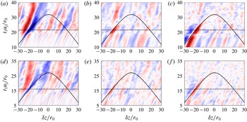
The correlations computed between the flow quantities at
 $r=0$
and pressure at
 $t_{2}u_{j}/r_{0}=40$
for
 $Re_{D}=3125$
and at
 $t_{2}u_{j}/r_{0}=35$
for
 $Re_{D}=12\,500$
are represented in figure 18 as functions of
 $\unicode[STIX]{x1D6FF}z$
and
 $t_{1}$
. The velocity–pressure correlations obtained between
 $t_{2}u_{j}/r_{0}=30$
and
 $50$
for
 $Re_{D}=3125$
and between
 $t_{2}u_{j}/r_{0}=30$
and
 $45$
for
 $Re_{D}=12\,500$
are displayed in the movies movie_fig18a and movie_fig18b. The dashed line represents the time of potential-core closing, and the solid line indicates a propagation at the ambient speed of sound between the centreline and near-field points. High levels of correlations, close to or higher than 0.2 for
 $Re_{D}=3125$
and 0.1 for
 $Re_{D}=12\,500$
, are found near the intersection of the two lines for negative separation distances
 $\unicode[STIX]{x1D6FF}z$
. This supports the presence of a sound source on the axis of both jets, radiating in the downstream direction, when the potential core disappears. The correlations are negative for
 $u_{z}^{\prime }$
and positive for
 $u_{z}^{\prime }u_{z}^{\prime }$
and
 $|\unicode[STIX]{x1D714}|^{\prime }$
. They can be related to the intermittent arrival of low-velocity vortical structures in the jet core. Strong correlations also appear before the time of potential-core closing for vorticity, and afterward for
 $u_{z}^{\prime }$
and
 $u_{z}^{\prime }u_{z}^{\prime }$
. They are due to the convection of the flow fluctuations in the jets, which will be illustrated later. These results are remarkably similar to those reported in Bogey & Bailly (Reference Bogey and Bailly2007) for Mach number 0.9, spatially developing jets at low and high Reynolds numbers.
Space–time correlations obtained between centreline quantities at
 $t=t_{1}$
and pressure fluctuations at
 $r=10r_{0}$
(a–c) at
 $t_{2}u_{j}/r_{0}=40$
for
 $Re_{D}=3125$
and (d–f) at
 $t_{2}u_{j}/r_{0}=35$
for
 $Re_{D}=12\,500$
: (a,d)
 ${\mathcal{C}}_{u_{z}^{\prime }p^{\prime }}$
, (b,e)
 ${\mathcal{C}}_{u_{z}^{\prime }u_{z}^{\prime }p^{\prime }}$
and (c,f)
 ${\mathcal{C}}_{|\unicode[STIX]{x1D714}|^{\prime }p^{\prime }}$
. The colour scale ranges from
 $-0.20$
to
 $0.20$
, from blue to red; —— propagation at the ambient speed of sound; – – –
 $t_{1}=t_{c}$
.

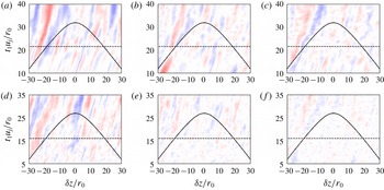
For comparison, the correlations obtained between the flow quantities at
 $r=r_{0}$
and pressure at
 $r=10r_{0}$
are represented in figure 19 in the same way as in figure 18. The correlation levels are significantly lower than those evaluated from the centreline fluctuations as in spatial jets (Bogey & Bailly Reference Bogey and Bailly2007). They do not exceed values of 0.07 for
 $Re_{D}=3125$
and 0.06 for
 $Re_{D}=12\,500$
. They even fail to emerge from the background noise in most cases, except for
 ${\mathcal{C}}_{u_{z}^{\prime }p^{\prime }}$
in figure 19(a) where an elongated correlation pattern similar, albeit very attenuated, to that visible in figure 18(a) appears for negative spatial separation distances. These results suggest that the sound source radiating in the downstream direction is not located in the centre of the mixing layers.
Space–time correlations obtained between quantities at
 $r=r_{0}$
and
 $t=t_{1}$
and pressure fluctuations at
 $r=10r_{0}$
(a–c) at
 $t_{2}u_{j}/r_{0}=40$
for
 $Re_{D}=3125$
and (d–f) at
 $t_{2}u_{j}/r_{0}=35$
for
 $Re_{D}=12\,500$
: (a,d)
 ${\mathcal{C}}_{u_{z}^{\prime }p^{\prime }}$
, (b,e)
 ${\mathcal{C}}_{u_{z}^{\prime }u_{z}^{\prime }p^{\prime }}$
and (c,f)
 ${\mathcal{C}}_{|\unicode[STIX]{x1D714}|^{\prime }p^{\prime }}$
. The colour scale ranges from
 $-0.20$
to
 $0.20$
, from blue to red; —— propagation at the ambient speed of sound; – – –
 $t_{1}=t_{c}$
.

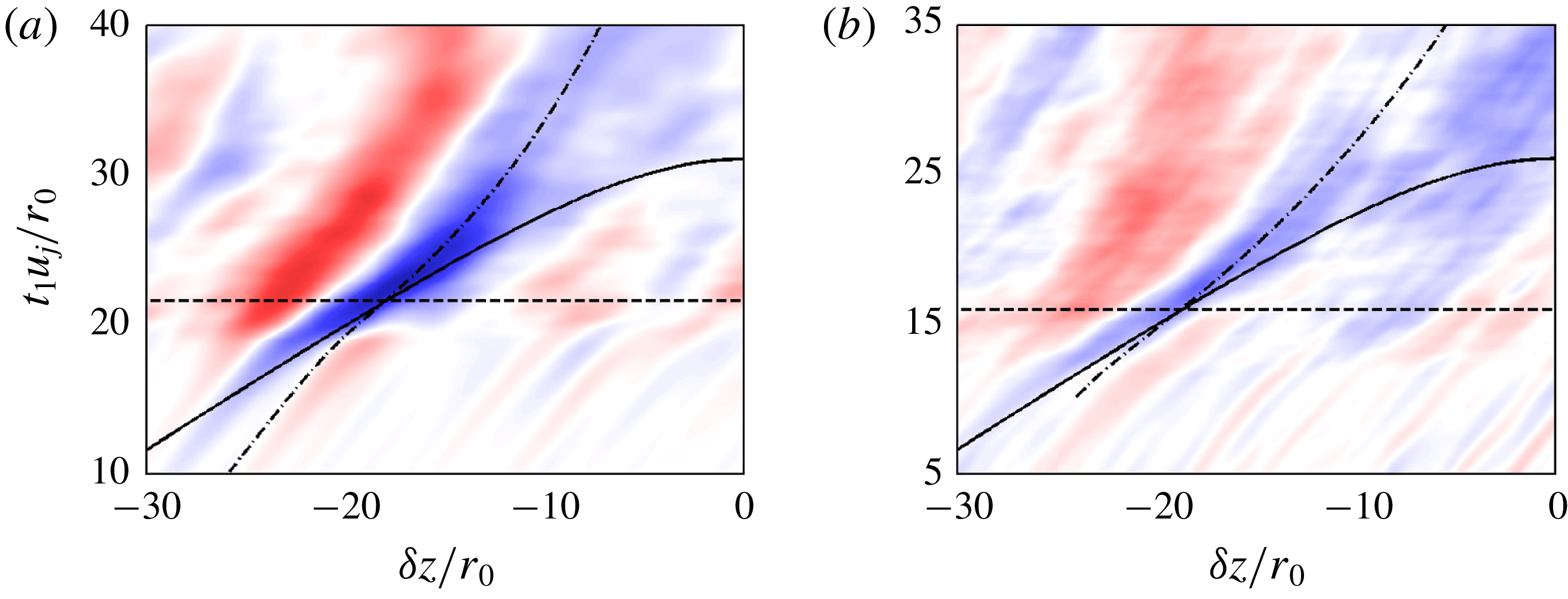
Coming back to the correlations computed from centreline flow quantities, the correlations
 ${\mathcal{C}}_{u_{z}^{\prime }p^{\prime }}$
are presented again in figure 20, together with mixed lines built from the convection velocities on the jet axis given in figure 11(b). The correlation spots coloured in blue turn out to follow these lines, revealing that their orientations result from the convection of the flow fluctuations in the jets (Bogey & Bailly Reference Bogey and Bailly2007). The time variations of these orientations are clearly seen in the corresponding movies.
Space–time correlations
 ${\mathcal{C}}_{u_{z}^{\prime }p^{\prime }}$
obtained between velocity fluctuations at
 $r=0$
and
 $t=t_{1}$
and pressure fluctuations at
 $r=10r_{0}$
(a) at
 $t_{2}u_{j}/r_{0}=40$
for
 $Re_{D}=3125$
and (b) at
 $t_{2}u_{j}/r_{0}=35$
for
 $Re_{D}=12\,500$
. The colour scale ranges from
 $-0.30$
to
 $0.30$
, from blue to red; —— propagation at the ambient speed of sound; – – –
 $t_{1}=t_{c}$
; –
 $\cdot$
–
 $\cdot$
trajectory based on the convection velocity on the jet axis.

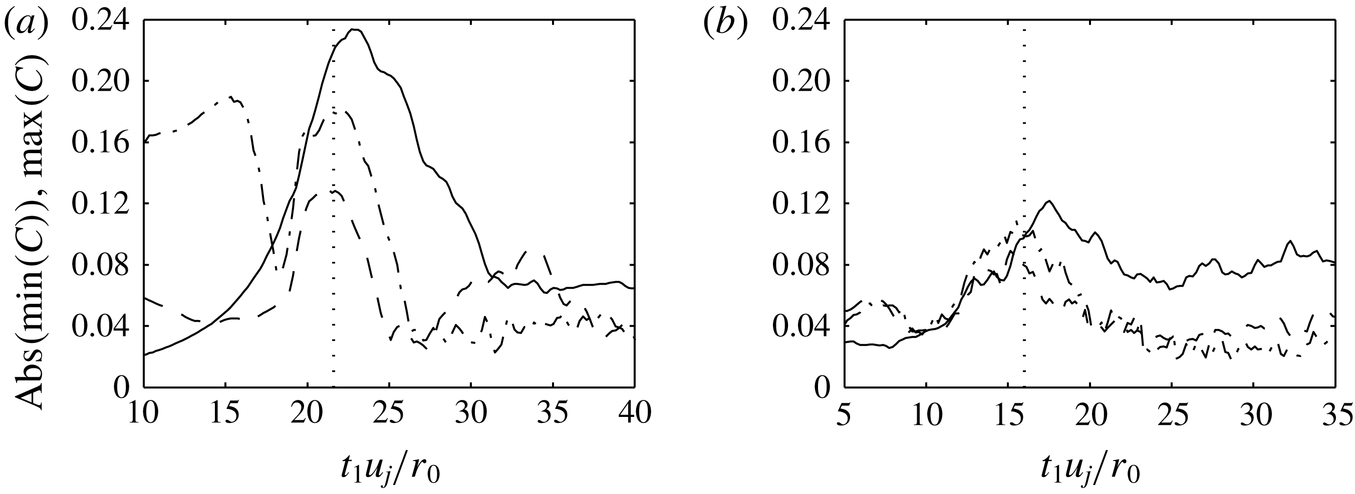
In order to provide more quantitative results, the peak values of correlations determined from centreline fluctuations at time
 $t_{1}$
and pressure fluctuations at
 $t_{2}u_{j}/r_{0}=40$
for
 $Re_{D}=3125$
and
 $t_{2}u_{j}/r_{0}=35$
for
 $Re_{D}=12\,500$
are plotted in figure 21 as a function of
 $t_{1}$
. Maximum values equal to 0.234, 0.132 and 0.180 for
 $Re_{D}=3125$
and to 1.122, 0.890 and 0.108 for
 $Re_{D}=12\,500$
are reached for
 $-{\mathcal{C}}_{u_{z}^{\prime }p^{\prime }}$
,
 ${\mathcal{C}}_{u_{z}^{\prime }u_{z}^{\prime }p^{\prime }}$
and
 ${\mathcal{C}}_{|\unicode[STIX]{x1D714}|^{\prime }p^{\prime }}$
, respectively, slightly after or at the time of potential-core closing. Significant levels are also obtained before
 $t=t_{c}$
for
 ${\mathcal{C}}_{|\unicode[STIX]{x1D714}|^{\prime }p^{\prime }}$
in figure 21(a). After the maximum values at
 $t\simeq t_{c}$
, moreover, the levels decrease rather slowly for
 $-{\mathcal{C}}_{u_{z}^{\prime }p^{\prime }}$
, supporting that the flow velocity feature correlating with the emitted sound waves persists long after the time of noise generation.
Representation of peak values of correlations between centreline quantities at
 $t=t_{1}$
and pressure fluctuations at
 $r=10r_{0}$
(a) at
 $t_{2}u_{j}/r_{0}=40$
for
 $Re_{D}=3125$
and (b) at
 $t_{2}u_{j}/r_{0}=35$
for
 $Re_{D}=12\,500$
: ——
 $|\text{min}({\mathcal{C}}_{u_{z}^{\prime }p^{\prime }})|$
, – – –
 $\max ({\mathcal{C}}_{u_{z}^{\prime }u_{z}^{\prime }p^{\prime }})$
, –
 $\cdot$
–
 $\cdot$
 $\max ({\mathcal{C}}_{|\unicode[STIX]{x1D714}|^{\prime }p^{\prime }})$
, as a function of
 $t_{1}$
;
 $\cdots \cdots$
 $t_{1}=t_{c}$
.

Finally, in the corresponding movies, the flow–noise correlation maps do not seem to depend much on the time of arrival of the acoustic waves at
 $r=10r_{0}$
. However, the correlation peak values gradually increase with time
 $t_{2}$
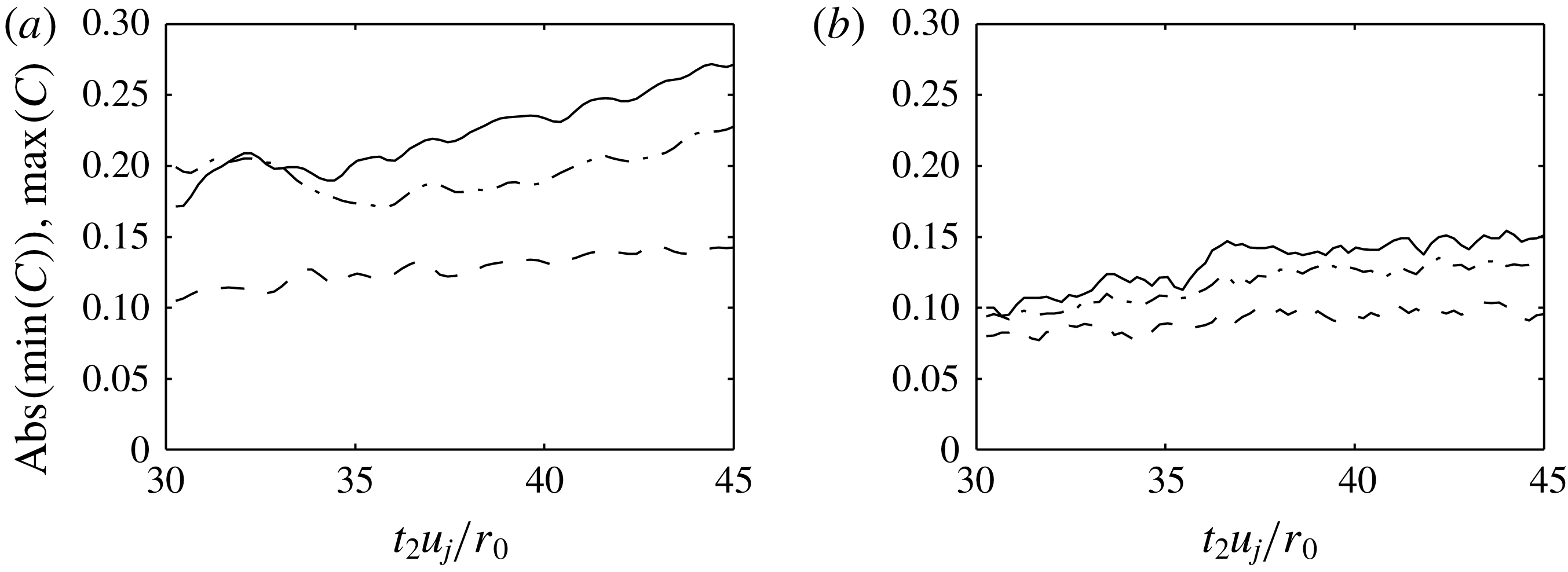
, as highlighted in figure 22. For
 $-{\mathcal{C}}_{u_{z}^{\prime }p^{\prime }}$
, for instance, they grow from 0.17 up to 0.27 for
 $Re_{D}=3125$
and from 0.10 up to 0.15 for
 $Re_{D}=12\,500$
between
 $t_{2}u_{j}/r_{0}=30$
and 45. Therefore, the flow–noise correlation levels are higher as the angle of radiation of the sound waves with respect to the flow direction is lower, which is in agreement with the experimental trends for spatial jets (Panda et al.
Reference Panda, Seasholtz and Elam2005).
Representation of peak values of correlations between centreline quantities at
 $t=t_{1}$
and pressure fluctuations at
 $r=10r_{0}$
at
 $t=t_{2}$
for (a)
 $Re_{D}=3125$
and (b)
 $Re_{D}=12\,500$
: ——
 $|\text{min}({\mathcal{C}}_{u_{z}^{\prime }p^{\prime }})|$
, – – –
 $\max ({\mathcal{C}}_{u_{z}^{\prime }u_{z}^{\prime }p^{\prime }})$
, –
 $\cdot$
–
 $\cdot$
 $\max ({\mathcal{C}}_{|\unicode[STIX]{x1D714}|^{\prime }p^{\prime }})$
, as a function of
 $t_{2}$
.

3.5 Conditional averaging of the jet flow and pressure fields
In order to visualize and better understand the noise generation mechanism related to the intermittent intrusion of turbulent structures in the core of the present jets, a conditional averaging method is applied in this section to the flow and acoustic fields provided by the simulations. The method consists in averaging a limited number of samples, selected using a trigger condition, in a signal or in a movie. It has been employed in the past in many studies to isolate a specific phenomenon from the background noise. For aeroacoustic purposes, it has enabled researchers, for example, to extract coherent structures and velocity events in mixing layers and jets (Dahan et al. Reference Dahan, Elias, Maulard and Perulli1978; Hileman et al. Reference Hileman, Thurow, Caraballo and Samimy2005; Camussi & Grizzi Reference Camussi and Grizzi2014), and acoustic components in the pressure fields of free and impinging subsonic and supersonic jets (Kearney-Fisher, Sinha & Samimy Reference Kearney-Fisher, Sinha and Samimy2013; Akamine et al. Reference Akamine, Okamoto, Teramoto, Okunuki and Tsutsumi2016). Thanks to this method, Kastner et al. (Reference Kastner, Samimy, Hileman and Freund2006), in particular, found that the rapid breakdown of the flow large-scale structures plays an important role in the generation of subsonic jet noise.
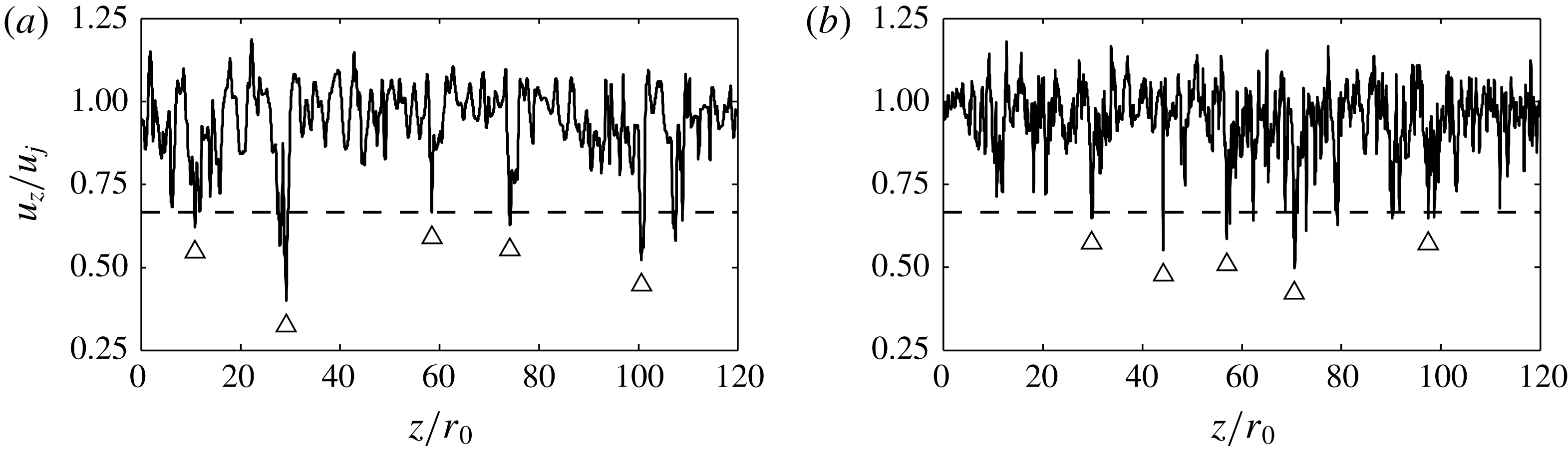
In the present work, the signal for the sample selection is the signal of axial velocity on the jet axis at the time
 $t_{c}$
of potential-core closing, and the trigger condition relies on the use of a lower threshold. These choices are motivated by the fact that centreline axial velocity strongly correlates with the near-field pressure fluctuations long after
 $t_{c}$
, and that it is negatively skewed, as shown in previous sections. The corresponding signals obtained in the first simulation runs of the two temporal jets are depicted in figure 23. For both Reynolds numbers, as expected from the profiles of skewness factors of velocity of figure 6(b), intermittent negative spikes of velocity much lower than the jet velocity, even below
 $0.5u_{j}$
in certain cases, can be seen. In the conditional averaging procedure, the trigger events are identified by detecting the minimum values of velocity below a threshold of
 $(2/3)u_{j}$
, yielding a difference of approximately three standard deviations below the mean value for the signals considered. This threshold value is chosen arbitrarily, but the use of other velocity thresholds, such as
 $0.60u_{j}$
and
 $0.75u_{j}$
, for example, does not change the results qualitatively but only quantitatively, as verified in appendix D. The trigger events separated by a distance of less than
 $10r_{0}$
are discarded to avoid sample overlapping. This reduces for instance the number of samples to 5 in the two signals of figure 23, and leads to a total number equal to 45 for
 $Re_{D}=3125$
and 43 for
 $Re_{D}=12\,500$
. The flow and pressure fields are then recorded over windows centred around the position
 $z_{c}$
of the trigger events, and the resulting snapshots are ensemble averaged. This is carried out at time
 $t_{c}$
, but also at previous and subsequent times using the same synchronization with the negative spikes of axial centreline velocity at time
 $t_{c}$
, in order to get access to the time evolution of the noise generation mechanism. The results obtained in the four azimuthal planes at
 $\unicode[STIX]{x1D703}=0$
,
 $\unicode[STIX]{x03C0}/2$
,
 $\unicode[STIX]{x03C0}$
and
 $3\unicode[STIX]{x03C0}/2$
are averaged, which allows us to increase convergence, but also to focus on the generation of the axisymmetric sound waves dominating in the jet near field, as shown by the spectra of figure 15. Despite the limited number of events selected, the averaged fields displayed in what follows clearly exhibit coherent features. This may be explained by the fact that these events are by far the most energetic ones in the flow.
Axial velocity obtained at
 $r=0$
and
 $t=t_{c}$
for (a)
 $Re_{D}=3125$
and (b)
 $Re_{D}=12\,500$
; – – –
 $u_{z}/u_{j}=2/3$
;
 $\triangle$
events selected for the conditional averaging.

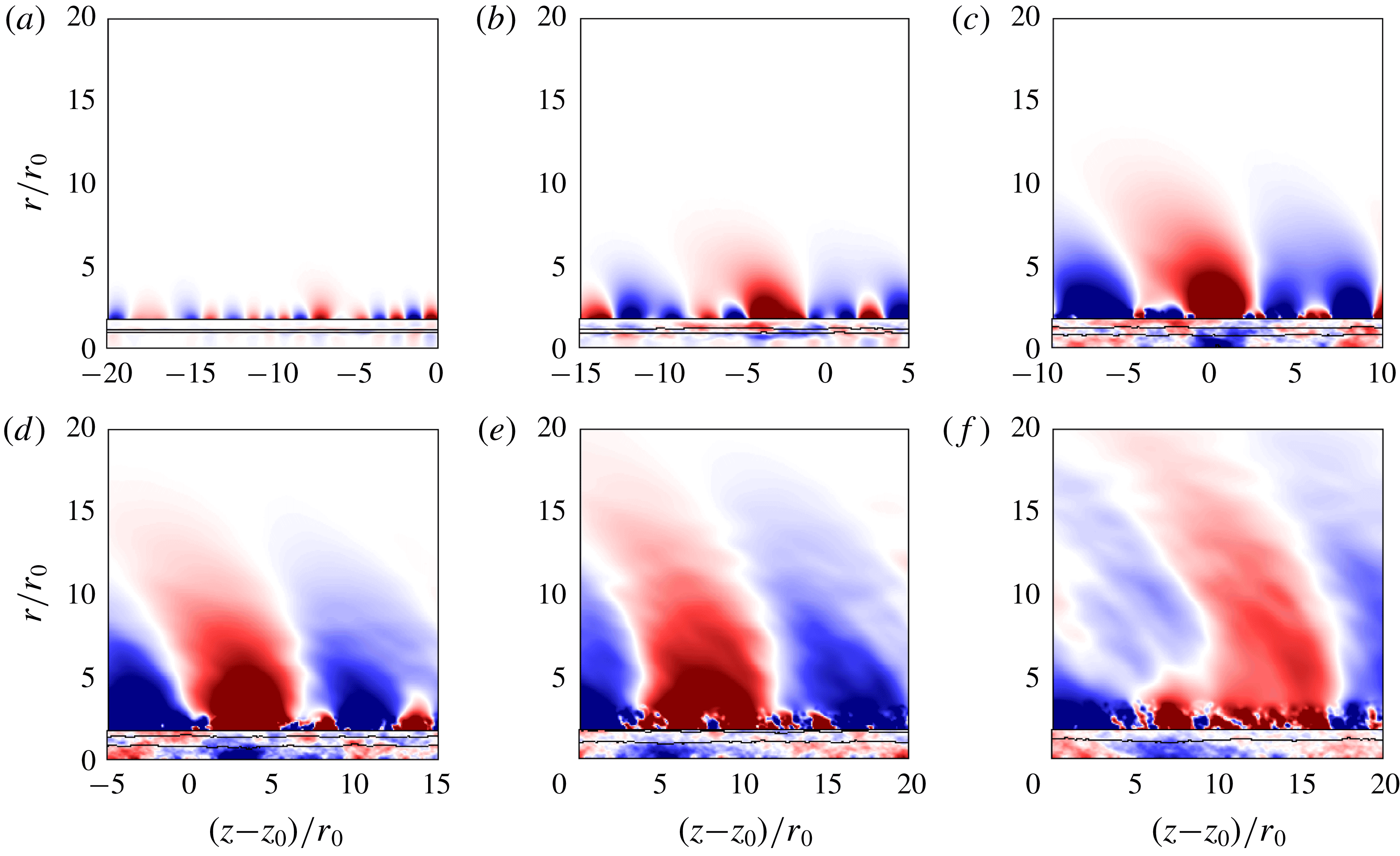
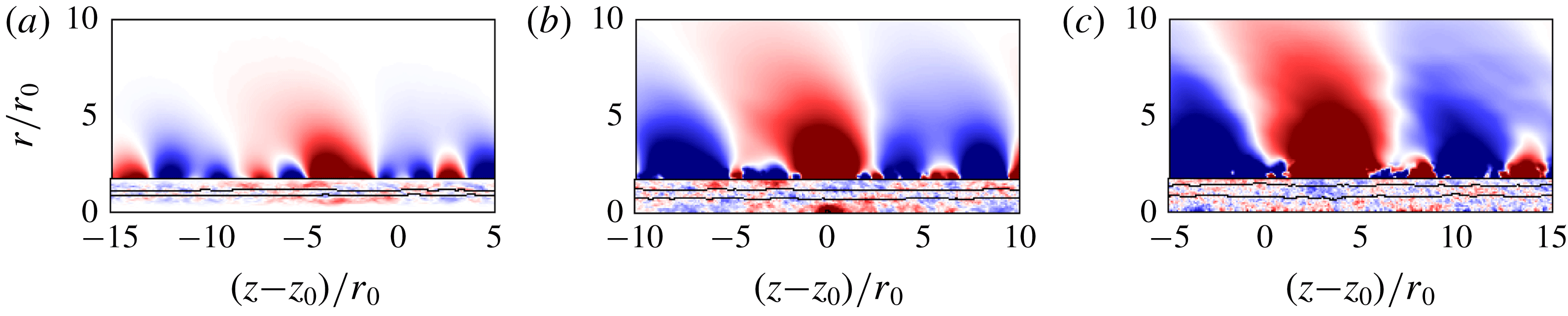
The conditional fields of velocity fluctuations in the jet flow and of the pressure fluctuations outside, obtained at six times distributed every
 $5r_{0}/u_{j}$
between
 $t_{c}-10r_{0}/u_{j}$
and
 $t_{c}+15r_{0}/u_{j}$
, are represented in figure 24 for
 $Re_{D}=3125$
and in figure 26 for
 $Re_{D}=12\,500$
; see also the corresponding movies movie_fig24 and movie_fig26. The conditional fields of vorticity fluctuations at
 $t_{c}-5r_{0}/u_{j}$
,
 $t_{c}$
and
 $t_{c}+5r_{0}/u_{j}$
are also given in figures 25 and 27. In the figures, velocity contours are drawn for the values of one third and two thirds of the mean centreline velocity in order to make the extent of the mixing layer visible. Similar features are observed for the two jets despite the difference in Reynolds number. The amplitudes are however lower in the pressure field for the higher Reynolds number case, in agreement with the results of § 3.3.
Representation of the fluctuations of axial velocity for
 $r\leqslant 1.75r_{0}$
and of pressure otherwise, obtained for
 $Re_{D}=3125$
at (a)
 $t_{c}-10r_{0}/u_{j}$
, (b)
 $t_{c}-5r_{0}/u_{j}$
, (c)
 $t_{c}$
, (d)
 $t_{c}+5r_{0}/u_{j}$
, (e)
 $t_{c}+10r_{0}/u_{j}$
and (f)
 $t_{c}+15r_{0}/u_{j}$
using conditional averaging; ——
 $u_{z}=(1/3)\langle u_{z}(r=0)\rangle$
and
 $u_{z}=(2/3)\langle u_{z}(r=0)\rangle$
. The colour scales range from
 $-0.075u_{j}$
up to
 $0.075u_{j}$
and from
 $-90$
up to
 $90~\text{Pa}$
, from blue to red.

Representation of the fluctuations of vorticity norm for
 $r\leqslant 1.75r_{0}$
and of pressure otherwise, obtained for
 $Re_{D}=3125$
at (a)
 $t_{c}-5r_{0}/u_{j}$
, (b)
 $t_{c}$
and (c)
 $t_{c}+5r_{0}/u_{j}$
using conditional averaging; ——
 $u_{z}=(1/3)\langle u_{z}(r=0)\rangle$
and
 $u_{z}=(2/3)\langle u_{z}(r=0)\rangle$
. The colour scales range from
 $-0.75u_{j}/r_{0}$
up to
 $0.75u_{j}/r_{0}$
and from
 $-90$
up to
 $90~\text{Pa}$
, from blue to red.

Representation of the fluctuations of axial velocity for
 $r\leqslant 1.75r_{0}$
and of pressure otherwise, obtained for
 $Re_{D}=12\,500$
at (a)
 $t_{c}-10r_{0}/u_{j}$
, (b)
 $t_{c}-5r_{0}/u_{j}$
, (c)
 $t_{c}$
, (d)
 $t_{c}+5r_{0}/u_{j}$
, (e)
 $t_{c}+10r_{0}/u_{j}$
and (f)
 $t_{c}+15r_{0}/u_{j}$
using conditional averaging; ——
 $u_{z}=(1/3)\langle u_{z}(r=0)\rangle$
and
 $u_{z}=(2/3)\langle u_{z}(r=0)\rangle$
. The colour scales range from
 $-0.075u_{j}$
up to
 $0.075u_{j}$
and from
 $-40$
up to
 $40~\text{Pa}$
, from blue to red.

Representation of the fluctuations of vorticity norm for
 $r\leqslant 1.75r_{0}$
and of pressure otherwise, obtained for
 $Re_{D}=12\,500$
at (a)
 $t_{c}-5r_{0}/u_{j}$
, (b)
 $t_{c}$
and (c)
 $t_{c}+5r_{0}/u_{j}$
using conditional averaging; ——
 $u_{z}=(1/3)\langle u_{z}(r=0)\rangle$
and
 $u_{z}=(2/3)\langle u_{z}(r=0)\rangle$
. The colour scales range from
 $-0.75u_{j}/r_{0}$
up to
 $0.75u_{j}/r_{0}$
and from
 $-40$
up to
 $40~\text{Pa}$
, from blue to red.

At the time of potential-core closing, in figures 24(c) and 25(b) for
 $Re_{D}=3125$
, and in figures 26(c) and 27(b) for
 $Re_{D}=12\,500$
, spots of strong negative and positive values are found, respectively, in the velocity and vorticity fields on the jet axis around
 $z=z_{c}$
, as expected due to the trigger condition used in the averaging procedure. In the pressure fields, lobes of positive fluctuations located at
 $z\simeq z_{c}$
and surrounded by two smaller lobes of negative fluctuations are noticed. They can be regarded as the traces of the turbulent structures in the jet near field (Arndt et al.
Reference Arndt, Long and Glauser1997).
The axial profiles of velocity and vorticity fluctuations at
 $r=0$
and of pressure fluctuations at
 $r=2.5r_{0}$
at
 $t=t_{c}$
are plotted in figure 28. For both jets, negative and positive spikes emerge for velocity and vorticity. They are centred around
 $z=z_{c}$
, are of length
 $0.6r_{0}$
, and exhibit extremum values of
 $-0.38u_{j}$
and
 $2.5u_{j}/r_{0}$
for
 $Re_{D}=3125$
and of
 $-0.36u_{j}$
and
 $3.5u_{j}/r_{0}$
for
 $Re_{D}=12\,500$
. At the same axial position, a hump of positive values peaking at 324 Pa for
 $Re_{D}=3125$
and at 215 Pa for
 $Re_{D}=12\,500$
is seen in the pressure profiles. It is the central part of the instability wave, of typical wavelength
 $12r_{0}$
, appearing in the pressure fields of figures 24(c) and 26(c). Therefore, when the potential core closes, the eruption of shear-layer vortical structures through the centre of the jet results in a velocity deficit and a vorticity excess in the flow, and in hydrodynamic pressure waves in its immediate vicinity.
Representation of the fluctuations of (a) axial velocity and (b) vorticity norm at
 $r=0$
, and of (c) pressure at
 $r=2.5r_{0}$
, obtained at
 $t=t_{c}$
using conditional averaging for ——
 $Re_{D}=3125$
and

 $Re_{D}=12\,500$
.

The evolutions of these flow and pressure patterns are revealed in figures 24–27 and in the corresponding movies. In both jets, before the potential-core closing, a spot of lower velocity and higher level of vorticity relative to the background flow field develops in the interfacial region between the mixing layer and the potential core. It is discernible at a very early stage, at
 $t_{c}-10r_{0}/u_{j}$
around
 $z=z_{c}-7r_{0}$
in the velocity fields of figures 24(a) and 26(a), and at
 $t_{c}-5r_{0}/u_{j}$
around
 $z=z_{c}-3.5r_{0}$
in the vorticity fields of figures 25(b) and 27(b). Its strength is characterized in figure 29 showing the extremum values of velocity and vorticity fluctuations at
 $r=0$
and between
 $r=0$
and
 $r=(2/3)r_{0}$
as a function of time. In absolute values, they first increase relatively slowly, but rise sharply after
 $t_{c}-3r_{0}/u_{j}$
. They reach a peak at
 $t\simeq t_{c}$
when the vortical spot arrives on the jet axis, and thereafter collapse. For
 $t\geqslant t_{c}$
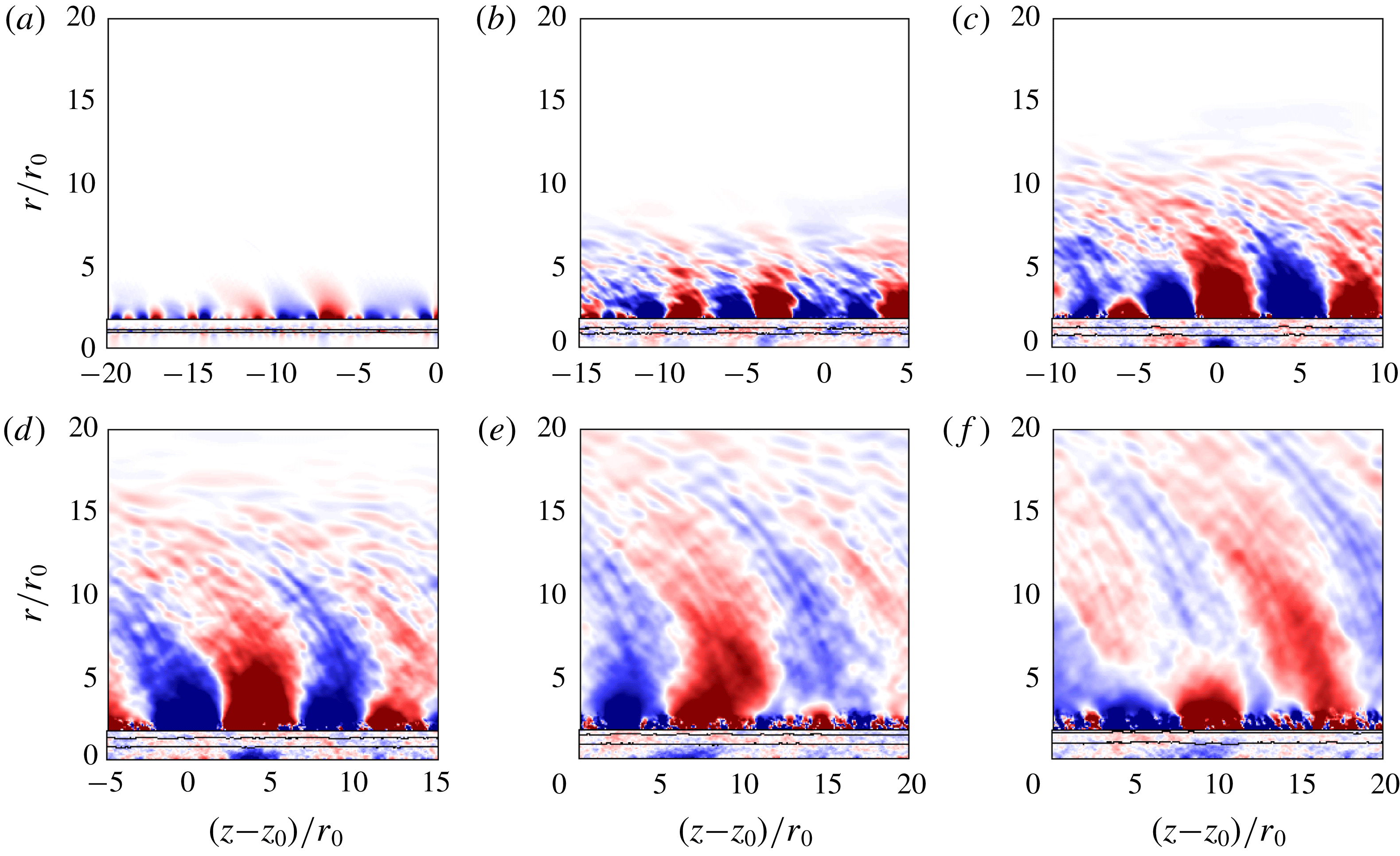
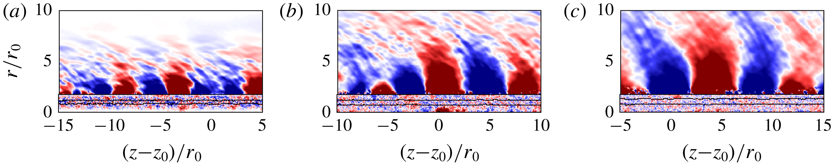
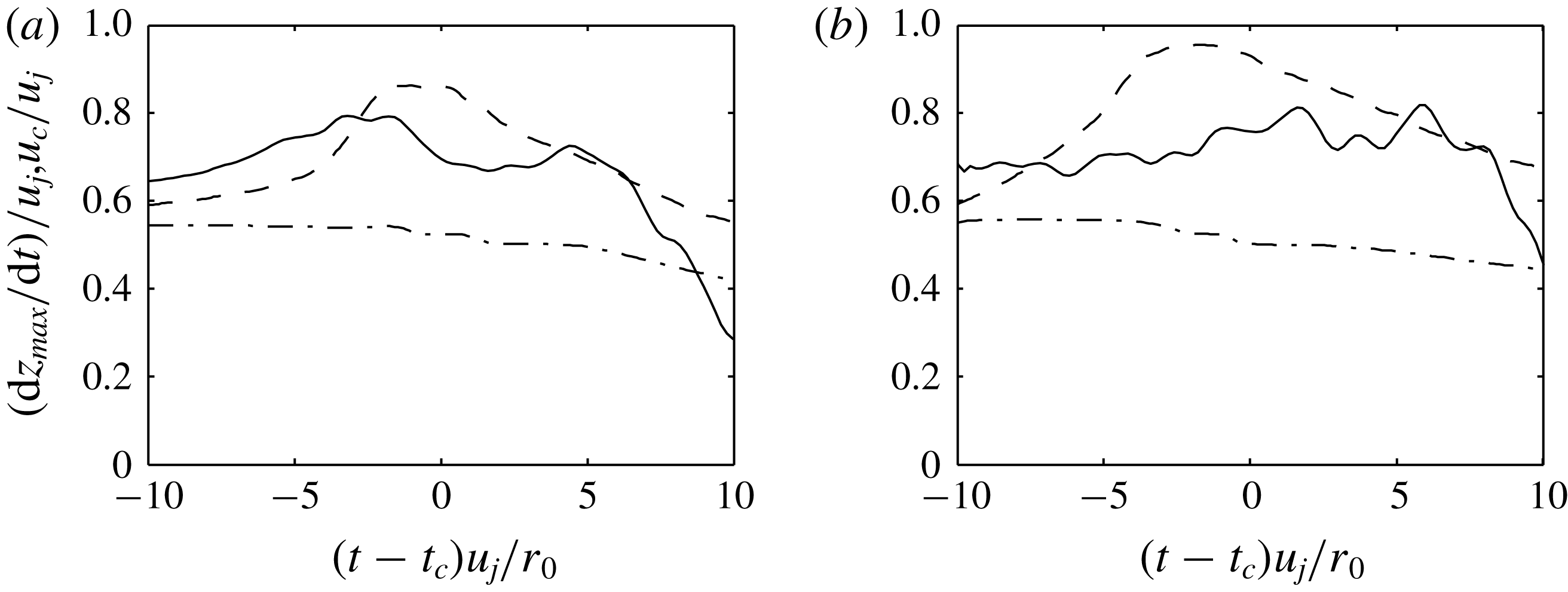
, the structure extracted by the conditional averaging also decelerates. It is thus located consecutively around
 $z=z_{c}$
,
 $z_{c}+4r_{0}$
,
 $z_{c}+7r_{0}$
and
 $z_{c}+9r_{0}$
in figure 26(c–f), for example. Moreover, the velocity deficit appears to persist over a long time period, and is still quite visible at
 $t_{c}+15r_{0}/u_{j}$
for both jets, with a large extent in the axial direction. On the contrary, the vorticity excess vanishes rapidly, and is hardly detectable at
 $t_{c}+5r_{0}/u_{j}$
in figures 25(c) and 27(c).
Time variations of (a) the minimum values of axial velocity fluctuations and (b) the maximum values of vorticity norm fluctuations obtained at
 $r=0$
for ——
 $Re_{D}=3125$
and

 $Re_{D}=12\,500$
, and between
 $r=0$
and
 $r=(2/3)r_{0}$
for – – –
 $Re_{D}=3125$
and

 $Re_{D}=12\,500$
using conditional averaging.

The development and disappearance of the high-vorticity spot on the high-velocity side of the mixing layer is accompanied by the growth and decay of a hydrodynamic pressure wave in the jet near field. To quantify this phenomenon, the normalized maximum values of pressure fluctuations obtained at
 $r=2.5r_{0}$
, as well as the corresponding values averaged over
 $2r_{0}\leqslant r\leqslant 3r_{0}$
, are represented in figure 30(a). For both jets, the two profiles are very similar to each other, indicating that the shape of the signal envelope does not depend appreciably on the radial position. In addition, the peak values of pressure fluctuations are achieved at
 $t\simeq t_{c}+2r_{0}/u_{j}$
. Interestingly, this is roughly the time when the correlations between the centreline velocity and the radiated noise are the strongest (refer to figure 21), suggesting that noise generation occurs at that moment.
Outside the jets, the emission and propagation of acoustic waves in the downstream direction are then clearly visible for both jets. One dominant wave of positive pressure, and two weaker waves of negative pressure on both sides, are radiated. They are attached to the flow velocity deficit at
 $t=t_{c}$
, but progressively move further away at later times as they travel at the speed of sound, more rapidly than the flow structures. The noise generation mechanism highlighted here strongly resembles that associated with a wave packet, exemplified in Tam et al. (Reference Tam, Viswanathan, Ahuja and Panda2008), Suzuki (Reference Suzuki2010) and Jordan & Colonius (Reference Jordan and Colonius2013). In the present work, it is clearly identified in a subsonic jet flow without resorting to any wave packet modelling.
The axial positions of the wave packets in the present jets, given in practice by those of the pressure peaks in the near field, are presented in figure 30(b) as a function of time. They are nearly identical for the two jets, regardless of the Reynolds number. Furthermore, they are very close to the positions of the minimum values of velocity in the flow, also depicted in the figure. This demonstrates the connection between the structure developing at the edge of the potential core and the hydrodynamic wave outside the jet flow. Both appear to travel at a rather uniform velocity between
 $t_{c}-10r_{0}/u_{j}$
and
 $t_{c}+5r_{0}/u_{j}$
, but subsequently at a velocity decreasing with time.
Time variations (a) of the maximum values of pressure fluctuations, normalized by their peak values, averaged over
 $2r_{0}\leqslant r\leqslant 3r_{0}$
for ——
 $Re_{D}=3125$
and

 $Re_{D}=12\,500$
and at
 $r=2.5r_{0}$
for – – –
 $Re_{D}=3125$
and

 $Re_{D}=12\,500$
, (b) of the axial positions of the pressure peaks averaged over
 $2r_{0}\leqslant r\leqslant 3r_{0}$
for ——
 $Re_{D}=3125$
and

 $Re_{D}=12\,500$
and of the minimum values of axial velocity between
 $r=0$
and
 $r=(2/3)r_{0}$
for ○
 $Re_{D}=3125$
and ○
 $Re_{D}=12\,500$
; – – – propagation at
 $0.8u_{j}$
.

The velocities estimated from the axial positions of the wave packets over segments of duration
 $5u_{j}/r_{0}$
are shown in figure 31. For both jets, despite the presence of oscillations, they are close to 65 per cent of the initial jet velocity at
 $t_{c}-10r_{0}/u_{j}$
, then gradually increase up to approximately
 $0.75u_{j}$
and finally fall down for
 $t>t_{c}+5r_{0}/u_{j}$
. Compared to the convection velocities calculated at
 $r=0$
and
 $r=r_{0}$
from velocity cross-correlations, they differ significantly. First, they are always higher than the convection velocity at
 $r=r_{0}$
, which can be related to the fact that the structure developing in the flow is not located in the centre of the mixing layer, as mentioned above. Second, at
 $t\simeq t_{c}$
, they are lower than the convection velocity at
 $r=0$
suggesting that in average, the structure accelerates less than it could have been expected when the potential core closes. Inversely, it appears to slow down suddenly shortly after.
Time variations of —— the velocities calculated from the positions of the near-field pressure peaks represented in figure 30(b) and of the convection velocities at – – –
 $r=0$
and –
 $\cdot$
–
 $\cdot$
 $r=r_{0}$
for (a)
 $Re_{D}=3125$
and (b)
 $Re_{D}=12\,500$
.

Finally, the present conditional fields provide explanations for the properties of the correlation maps obtained between flow and acoustic fluctuations for the temporal jets, but also for spatially developing jets (Schaffar Reference Schaffar1979; Bogey & Bailly Reference Bogey and Bailly2007). The absence of velocity deficit and vorticity excess in the mixing layer seems to be responsible for the negligible correlations computed from the flow signals at
 $r=r_{0}$
. The persistence of a velocity deficit over a long period and the rapid disappearance of a vorticity excess on the jet axis may also be the reasons for which the correlations based on the centreline signals remain significant long after the time of sound generation for velocity but not for vorticity. Lastly, several pressure waves of alternating sign are emitted during the noise generation process, which may be the cause of the presence of the multiple spots of notable level in the correlation fields.
4 Conclusion
In this paper, noise generation in temporally developing subsonic round jets is investigated. For that purpose, the flow and the near pressure fields computed for isothermal jets at a Mach number of 0.9 and Reynolds numbers of 3125 and 12 500 using direct numerical simulation are detailed. Cross-correlations between the two fields are also calculated in order to localize possible sound sources in the jets. Overall, despite the difference in Reynolds number, leading to a more rapid flow development and more high-frequency components for the higher Reynolds number jet, the results for the two jets are very similar. In both cases, when the jet potential core closes, shear-layer turbulent structures intermittently intrude inside the jet, and high-amplitude low-frequency waves are radiated in the downstream direction. These waves are significantly correlated with the axial velocity and vorticity fluctuations on the jet centreline. These results suggest that the mechanism responsible for the downstream noise component of spatially developing subsonic jets is also encountered in temporal jets. Therefore, it appears not to depend on the presence of a potential core of finite length, of a nozzle or on the streamwise spreading of the jet flow, but to be linked to the physics of the interactions and merging of parallel mixing layers.
In the present jets, that mechanism is extracted by a procedure of conditional averaging of the flow and sound fields using a sample synchronization with the minimum values of centreline velocity at the time of potential-core closing
 $t_{c}$
. It occurs over a long time period, and evolves large-scale coherent features of the flow. In summary, a spot of lower velocity and higher level of vorticity relative to the background flow field develops at the inner edge of the mixing layer, reaches a peak intensity on the jet axis at
 $t_{c}$
, and then disappears. Simultaneously, a hydrodynamic wave packet grows and decays in the near pressure field. Both travel at a velocity initially slightly increasing with time, but rapidly decreasing shortly after
 $t_{c}$
. In the acoustic field, sound waves are emitted in the flow direction from the wave packet. Further studies will be based on extra post-processing of the present simulation data. Additional simulations of temporally developing jets, at different Mach numbers for instance, will also be performed in order to get more information about the noise generation mechanism revealed in this work. Finally, it will be necessary to go back and consider spatial jets to determine whether that mechanism can be isolated in such flows.
Acknowledgements
The present work was granted access to the High-Performance-Computing resources of FLMSN (Fédération Lyonnaise de Modélisation et Sciences Numériques), partner of EQUIPEX EQUIP@MESO, and of IDRIS (Institut du Développement et des Ressources en Informatique Scientifique) under the allocation 2016-2a0204 made by GENCI (Grand Equipement National de Calcul Intensif). It was performed within the framework of the Labex CeLyA of Université de Lyon, operated by the French National Research Agency (grant no. ANR-10-LABX-0060/ANR-11-IDEX-0007).
Supplementary movies
Representation of vorticity norm for
 $r\leqslant 3r_{0}$
and of pressure fluctuations otherwise, obtained for
 $Re_{D}=50\,000$
at (a)
 $tu_{j}/r_{0}=20$
and (b)
 $tu_{j}/r_{0}=45$
. The colour scales range up to the level of
 $5u_{j}/r_{0}$
for vorticity, and from
 $-200$
to
 $200~\text{Pa}$
for pressure, from blue to red.

Supplementary movies are available at https://doi.org/10.1017/jfm.2018.864.
Appendix A
In this first appendix, the extra simulation of a temporal jet at
 $Re_{D}=50\,000$
is reported. The jet flow is initially set up and forced as described in § 2.1 for the two jets at lower Reynolds numbers considered in this study. Following the variations of
 $\unicode[STIX]{x1D6FF}_{\unicode[STIX]{x1D703}}/r_{0}$
with the Reynolds number, in particular, the momentum thickness of the mixing layer is equal to
 $\unicode[STIX]{x1D6FF}_{\unicode[STIX]{x1D703}}=0.0089r_{0}$
at
 $t=0$
, which is twice as thin as for the jet at
 $Re_{D}=12\,500$
. In the simulation, the grid is finer compared to that defined in § 2.3 for the two other jets to keep a very high resolution. It contains
 $n_{r}\times n_{\unicode[STIX]{x1D703}}\times n_{z}=657\times 1024\times 3200=2.2$
billion points, and is characterized by mesh spacings of
 $\unicode[STIX]{x0394}r=0.003r_{0}$
at
 $r=r_{0}$
and
 $\unicode[STIX]{x0394}r=0.0125r_{0}$
on the jet axis, and of
 $\unicode[STIX]{x0394}z=0.0125r_{0}$
. Therefore, it extends only up to
 $z=40r_{0}$
in the axial direction. A total number of 18 600 iterations are performed, for a final time of
 $t=50r_{0}/u_{j}$
. Only one run is carried out, preventing the presentation of statistical results.
Space correlations of axial velocity fluctuations obtained at (a,c)
 $r=0$
and (b,d)
 $r=r_{0}$
for (a,b)
 $Re_{D}=3125$
and (c,d)
 $Re_{D}=12\,500$
: at ——
 $t=10r_{0}/u_{j}$
, – – –
 $t=20r_{0}/u_{j}$
, –
 $\cdot$
–
 $\cdot$
 $t=30r_{0}/u_{j}$
,
 $\cdots \cdots$
 $t=40r_{0}/u_{j}$
.

Results obtained for
 $Re_{D}=3125$
from —— 5 and – – – 10 runs and for
 $Re_{D}=12\,500$
from


 $r=0$
, (b) peak value of axial turbulence intensity, (c) r.m.s. value of pressure fluctuations at
 $r=10r_{0}$
, and (d) power spectral densities of pressure fluctuations at
 $r=10r_{0}$
at
 $tu_{j}/r_{0}=45$
for
 $Re_{D}=3125$
and
 $tu_{j}/r_{0}=40$
for
 $Re_{D}=12\,500$
.

Snapshots of the vorticity norm and pressure fluctuations obtained in the
 $(z,r)$
plane at
 $tu_{j}/r_{0}=20$
and 45, that is just before and well after the time of potential-core closing, are shown in figure 32 and in the movie movie_fig32. Large-scale hydrodynamic waves and acoustic waves of short wavelength are found in the pressure field at both times. Above all, low-frequency sound waves are seen to propagate in the downstream direction at the later time. They strongly resemble and have amplitudes similar to those obtained for the jet at
 $Re_{D}=12\,500$
in figure 3. These results suggest that the downstream noise component obtained for the temporal jets at
 $Re_{D}=3125$
and
 $Re_{D}=12\,500$
persists at higher Reynolds numbers. This component also seems not to depend significantly on the shear-layer initial momentum thickness.
Appendix B
In this second appendix, the space correlations of axial velocity fluctuations obtained at
 $r=0$
and
 $r=r_{0}$
in the two temporal jets at
 $Re_{D}=3125$
and
 $Re_{D}=12\,500$
at times
 $tr_{0}/u_{j}=10$
, 20, 30 and 40 are represented in figure 33 as a function of separation distance
 $\unicode[STIX]{x1D6FF}z$
up to
 $\unicode[STIX]{x1D6FF}z=60r_{0}$
, which is half the axial extent of the computational domain, in order to examine the influence of the periodic conditions, and to detect a possible bias due to these conditions. For separation distances
 $\unicode[STIX]{x1D6FF}z>5r_{0}$
, the correlation levels at
 $r=0$
in figure 33(a,c) are small, typically below 0.05, and decrease with time as the jets develop. The levels at
 $r=r_{0}$
in figure 33(b,d) are much smaller, and even negligible, due to better convergence thanks to the averaging in the azimuthal direction. In all cases, in particular, no correlation hump emerges around
 $\unicode[STIX]{x1D6FF}z=60r_{0}$
,
 $30r_{0}$
and
 $15r_{0}$
, corresponding to one half, one quarter and one eighth of the domain size. Therefore, the periodic conditions in the axial direction do not appear to distort the jet flow development.
Velocity and pressure fluctuations obtained at
 $t=t_{c}+12r_{0}/u_{j}$
for
 $Re_{D}=3125$
by conditional averaging using thresholds of (a)
 $u_{z}=0.60u_{j}$
, (b)
 $u_{z}=(2/3)u_{j}$
and (c)
 $u_{z}=0.75u_{j}$
for the event detection. The colour scales range from
 $-0.075u_{j}$
up to
 $0.075u_{j}$
and from
 $-90$
up to
 $90~\text{Pa}$
, from blue to red.

Velocity and pressure fluctuations obtained at
 $t=t_{c}+12r_{0}/u_{j}$
for
 $Re_{D}=12\,500$
by conditional averaging using thresholds of (a)
 $u_{z}=0.60u_{j}$
, (b)
 $u_{z}=(2/3)u_{j}$
and (c)
 $u_{z}=0.75u_{j}$
for the event detection. The colour scales range from
 $-0.075u_{j}$
up to
 $0.075u_{j}$
and from
 $-40$
up to
 $40~\text{Pa}$
, from blue to red.

Appendix C
In this third appendix, the time variations of mean axial velocity on the jet centreline, of peak axial turbulence intensity and of the r.m.s. values of pressure fluctuations at
 $r=10r_{0}$
, and pressure spectra at
 $r=10r_{0}$
calculated from 5 runs and from 10 runs are compared in figure 34 for the two jets at
 $Re_{D}=3125$
and
 $Re_{D}=12\,500$
, in order to check the sensitivity of the results to the number of runs performed for each jet using different initial perturbations. In all cases, the solutions are identical or very similar to each other. Therefore, the statistical results seem to be well converged in the present study.
Appendix D
In this final appendix, the influence of the threshold value arbitrarily chosen for the conditional averaging in § 3.5 is illustrated. The fields of velocity and pressure fluctuations obtained at
 $t=t_{c}+12r_{0}/u_{j}$
using velocity thresholds of
 $u_{z}=0.60u_{j}$
,
 $(2/3)u_{j}$
and
 $0.75u_{j}$
on the jet axis for the event detection at
 $t=t_{c}$
are shown in figure 35 for the jet at
 $Re_{D}=3125$
and in figure 36 for the one at
 $Re_{D}=12\,500$
. For both jets, the use of different threshold values is found not to change the results qualitatively. However, lowering the threshold results in an increase of the levels, because only the most energetic events are averaged in this case. For
 $Re_{D}=12\,500$
, for example, the extremum values of velocity fluctuations at
 $r=0$
and of pressure fluctuations at
 $r=5r_{0}$
at
 $t=t_{c}+12r_{0}/u_{j}$
are equal to
 $-0.033u_{j}$
and
 $25.3~\text{Pa}$
using a threshold of
 $u_{z}=0.75u_{j}$
but to
 $-0.079u_{j}$
and
 $56.6~\text{Pa}$
using
 $u_{z}=0.60u_{j}$
. More oscillations also appear: compare for instance figures 35(a) and 35(c). Given that the numbers of events detected in the two jets are equal to 62 and 68 using a velocity threshold of
 $u_{z}=0.75u_{j}$
, 45 and 43 using
 $u_{z}=(2/3)u_{j}$
, but only 26 and 23 using
 $u_{z}=0.60u_{j}$
, they are due to poorer convergence.