


1. Introduction
An important outcome of the first similarity hypothesis of Kolmogorov (Reference Kolmogorov1941) (K41) is that the normalized moments of  $\partial u_1/\partial x_1$, i.e.
 \begin{equation} {F_{n + 1}} = \frac{{\overline{{{\left({\dfrac{{\partial {u_1}}}{{\partial {x_1}}}} \right)}^{n + 1}}} }}{{{{\overline{{{\left( {\dfrac{{\partial {u_1}}}{{\partial {x_1}}}} \right)}^2}} }^{(n + 1)/2}}}}, \end{equation}
are constant ( $n = 1, 2, 3\ldots$) at very large
 $Re_\lambda$ (=
 ${u_1'}\lambda /\nu$, where
 $\lambda$ is the longitudinal Taylor microscale
 $u_1'/ (\partial u_1/\partial x_1)'$,
 $\nu$ is the fluid kinematic viscosity and a prime denotes a root-mean-square value), while the refined similarity hypothesis of Kolmogorov (Reference Kolmogorov1962) (K62) predicts a power-law increase for
 $|{F_{n + 1}} |$ (by definition,
 $F_2=1$) with
 ${Re_\lambda }$ (e.g. Gibson, Stegen & Williams Reference Gibson, Stegen and Williams1970; Wyngaard & Tennekes Reference Wyngaard and Tennekes1970; Van Atta & Antonia Reference Van Atta and Antonia1980; Sreenivasan & Antonia Reference Sreenivasan and Antonia1997; Davidson Reference Davidson2004; Ishihara, Gotoh & Kaneda Reference Ishihara, Gotoh and Kaneda2009), viz.
 \begin{equation} |F_{n+1}|\sim {Re_\lambda^{\alpha_{(n+1)}}} \quad (\alpha>0). \end{equation}
In (1.1),  $u_1$,
 $u_2$ and
 $u_3$ are the velocity fluctuations along the
 $x_1$,
 $x_2$ and
 $x_3$ directions, respectively, and the overbar denotes time averaging.
In fact,  $Re_\lambda$ is required to be very large so that, when
 $n \geq 2$,
 ${F_{n+1}}$ is not affected by large-scale forcing and either (1.1) or (1.2) holds. However, many turbulent flows encountered in practical situations are characterized by a low to moderate
 $Re_\lambda$ and thus the influence of the large-scale forcing, which may differ from flow to flow, on
 ${F_{n+1}}$ may linger. An understanding of this influence is of major importance in turbulence research because only when this influence disappears can we make meaningful assessments with regard to (1.1) or (1.2). One question then naturally arises: how do we quantify the effect of large-scale forcing on
 ${F_{n+1}}$ in a given flow, for example, in shearless grid turbulence? Batchelor & Townsend (Reference Batchelor and Townsend1947) were the first to derive an equation for
 ${F_{3}}$ in shearless grid turbulence, viz.
 \begin{equation} - U_1\frac{{\textrm{d} \overline\varepsilon_{iso} }}{{\textrm{d}\kern0.7pt x}} = \frac{7}{{3\sqrt {15} }} \frac{{{{\overline\varepsilon_{iso} }^{3/2}}}}{{{\nu ^{1/2}}}}\left[F_{3} + 2\frac{G}{{{Re_\lambda }}}\right], \end{equation}
where  $U_1$ is the (constant) mean velocity in the
 $x_1$ direction. In (1.3),
 $\overline \varepsilon _{iso}$ (
 $=15\nu \overline {(\partial u_{1}/\partial x_{1})^2 }$) is the isotropic energy dissipation rate and G is the non-dimensional enstrophy destruction coefficient of
 $\overline \varepsilon _{iso}$
 \begin{equation} G = \overline{u_1^2 } \frac{{\overline{(\partial ^2 u_1 /\partial x_1^2 )^2 } }}{\overline{(\partial u_1 /\partial x_1 )^2 }^2}. \end{equation}
Recently, Thiesset, Antonia & Djenidi (Reference Thiesset, Antonia and Djenidi2014), Antonia et al. (Reference Antonia, Tang, Djenidi and Danaila2015) and Tang et al. (Reference Tang, Antonia, Djenidi, Abe, Zhou, Danaila and Zhou2015a,Reference Tang, Antonia, Djenidi and Zhoub) extended the work of Batchelor & Townsend (Reference Batchelor and Townsend1947) to various turbulent flows, i.e. grid turbulence, along the axis in the self-preserving far-field of a round jet, along the centreline of a fully developed channel flow and a far-wake of a circular cylinder. They showed that, in each flow, the transport equation for  $\overline \varepsilon _{iso}$ can be written as
 \begin{equation} F_3 + 2\frac{G}{{{Re_\lambda }}}=\frac{C}{{{Re_\lambda }}}, \end{equation}
where the analytical expression for  $C$, which reflects the effect of large-scale forcing on
 $F_3$, differs from flow to flow. In shearless grid turbulence,
 $C={{90}}/{{7(1 + 2R)}}({{({-m + 1})}/{-m}})$ with
 $R = \overline {{u_2^2}} /\overline {{u_1^2}}$ and
 $m$ is a power-law decay exponent for the longitudinal velocity variance, viz.
 $\overline {u_1^2} \sim x_1^{m}$, while
 $C={{90}}/{{7(2 + R)}}$ on the axis of a far-field of a self-preserving round jet (Thiesset et al. Reference Thiesset, Antonia and Djenidi2014; Antonia et al. Reference Antonia, Tang, Djenidi and Danaila2015). For shearless grid turbulence, Djenidi, Antonia & Tang (Reference Djenidi, Antonia and Tang2019) further showed that the effect of the large-scale forcing on
 $F_4$ can be recast in the form
 $(100/3)\times F_3/Re_\lambda$ when
 $m=-1$ and thus should tend to zero when
 ${Re_\lambda }$ is sufficiently large. To our knowledge, however, there has been no attempt to quantify the effect of the large-scale forcing on
 $F_{n+1}$ for
 $n>3$. Therefore, the major objective of this paper is to develop an analytical framework based on the Navier–Stokes (N–S) equations which should allow the effect on
 $F_{n+1}$ of the large-scale forcing, associated with the combined actions of streamwise advection and mean shear, to be quantified in grid turbulence. It should be noted that the large-scale effect acts at various scales of motion, as seen for example in the transport equation of the second-order velocity structure function (e.g. Danaila, Anselmet & Antonia Reference Danaila, Anselmet and Antonia2002). However, their impact decreases with decreasing scale. Thus, for convenience, we use hereafter the terminology ‘large-scale effect’ when referring to advection and mean shear phenomena.
In the sense implied by (1.1) and (1.2), local isotropy should apply to all statistical moments. The exact isotropic relations between different components of the fourth-order tensor  $\overline {({{\partial {u_i}}}/{{\partial {x_p}}})({{\partial {u_j}}}/{{\partial {x_q}}})}$ (the second-order moment) have often been used to test local isotropy (Mestayer Reference Mestayer1982; Browne, Antonia & Shah Reference Browne, Antonia and Shah1987; Antonia, Kim & Browne Reference Antonia, Kim and Browne1991; Kim & Antonia Reference Kim and Antonia1993; Saddoughi & Veeravalli Reference Saddoughi and Veeravalli1994; Gotoh, Fukayama & Nakano Reference Gotoh, Fukayama and Nakano2002; Lavoie et al. Reference Lavoie, Burattini, Djenidi and Antonia2005; Thiesset, Danaila & Antonia Reference Thiesset, Danaila and Antonia2013a). Siggia (Reference Siggia1981) showed that in isotropic turbulence, all fourth-order velocity derivative moments can be expressed in terms of four invariants
 \begin{equation} \left.\begin{gathered} {I_1} = \overline{{{(\textrm{tr}({s^2}))}^2}} = \overline{{{(s_1^2 + s_2^2 + s_3^2)}^2}}, \\ {I_2} = \overline{{\omega ^2}\textrm{tr}({s^2})} = \overline{(\omega _1^2 + \omega _2^2 + \omega _3^2)(s_1^2 + s_2^2 + s_3^2)}, \\ {I_3} = \overline{{\omega ^2}{s_{ij}}{s_{jk}}{\omega _k}} = \overline{\omega _1^2s_1^2 + \omega _2^2s_2^2 + \omega _3^2s_3^2},\\ {I_4} = \overline{{{({\omega ^2})}^2}} = \overline{{{(\omega _1^2 + \omega _2^2 + \omega _3^2)}^2}}, \end{gathered}\right\} \end{equation}
where  $\omega$ is the module of the vorticity vector, s is the strain tensor and
 ${\textrm {tr}({s^2})}$ is the trace of the contracted product of s with itself. Although the dependence of
 $I_1$,
 $I_2$,
 $I_3$ and
 $I_4$ on
 $Re_\lambda$ has been examined in homogeneous isotropic turbulence and the outer region of a turbulent boundary layer over a smooth wall (e.g. Kerr Reference Kerr1985; Tsinober, Kit & Dracos Reference Tsinober, Kit and Dracos1992; Zhou & Antonia Reference Zhou and Antonia2000b; Ishihara et al. Reference Ishihara, Kaneda, Yokokawa, Itakura and Uno2007), there is no attempt to test the isotropic fourth-order velocity derivative moments as a function of four invariants. Instead, for the high-order moments, local isotropy tests have often focused on the behaviour of normalized odd moments of transverse velocity derivatives, defined as
 \begin{equation} {F_{y,n + 1}} = \frac{{\overline{{{\left( {\dfrac{{\partial {u_1}}}{{\partial {x_2}}}} \right)}^{n + 1}}} }}{{{{\overline{{{\left( {\dfrac{{\partial {u_1}}}{{\partial {x_2}}}} \right)}^2}} }^{(n + 1)/2}}}}, \end{equation}
(with  $n= 2, 4$ and 6) which should be zero if local isotropy is satisfied. However, available data, primarily in nearly sheared grid turbulence, indicate that small-scale anisotropy persists to very high Reynolds numbers. For example, Schumacher, Sreenivasan & Yeung (Reference Schumacher, Sreenivasan and Yeung2003) collected available data for
 $F_{y,3}$ and showed that, although
 $F_{y,3}$ decreases as
 $Re_\lambda$ increases, it is still not zero (
 $\approx$0.2) at
 $Re_\lambda \approx 1000$. Shen & Warhaft (Reference Shen and Warhaft2000) showed that, allowing for the scatter (in the range
 ${\approx }10{\sim}25$),
 $F_{y,5}$ does not show any obvious dependence on
 $Re_\lambda$ over the range
 $100< Re_\lambda <1000$ (see also Schumacher et al. Reference Schumacher, Sreenivasan and Yeung2003). Shen & Warhaft (Reference Shen and Warhaft2000) showed that
 $F_{y,7}$ actually increases with
 $Re_\lambda$ (
 $F_{y,7} \sim Re_\lambda ^{0.63}$). This raises the question: how does the departure from zero of
 ${F_{y,n + 1}}$ affect other small-scale quantities? This will be addressed in the present paper.
2. Theoretical considerations
The dynamic equation for the velocity fluctuation  $u_i$ is given by (e.g. Pope Reference Pope2000)
 \begin{equation} \frac{{\partial {u_i}}}{{\partial t}} + {U_j}\frac{{\partial {u_i}}}{{\partial {x_j}}} + {u_j} \frac{{\partial {u_i}}}{{\partial {x_j}}} + {u_j}\frac{{\partial {{U}_i}}}{{\partial {x_j}}} - \frac{{\partial \overline{{u_i}{u_j}} }}{{\partial {x_j}}} + \frac{{\partial p}}{{\partial {x_i}}} - \nu \frac{\partial }{{\partial {x_j}}}\frac{{\partial {u_i}}}{{\partial {x_j}}} = 0 \end{equation}
In (2.1),  $U_1$,
 $U_2$ and
 $U_3$ are the mean velocities in the
 $x_1$,
 $x_2$ and
 $x_3$ directions, respectively, and
 $p$ is the instantaneous kinematic pressure. Note that
 $i=1,2,3$ and, unless otherwise noted, only the repeated index
 $j$ indicates summation. We first differentiate (2.1) with respect to
 $x_k$ (
 $k=1,2,3$), multiply the resulting equation by
 $({\partial u_i /\partial {x_k}})^n$ (
 $n=1,2,3 \ldots$) and then average to finally obtain:
 \begin{align} & \overline{{{\left( {\frac{{\partial {u_i}}}{{\partial {x_k}}}} \right)}^n} \frac{\partial }{{\partial {x_k}}}\frac{{\partial {u_i}}}{{\partial t}}} + \frac{{\partial {{U}_j}}}{{\partial {x_k}}} \overline{{{\left( {\frac{{\partial {u_i}}}{{\partial {x_k}}}} \right)}^n} \frac{{\partial {u_i}}}{{\partial {x_j}}}} + {{U}_j} \overline{{{\left( {\frac{{\partial {u_i}}}{{\partial {x_k}}}} \right)}^n} \frac{\partial }{{\partial {x_k}}}\frac{{\partial {u_i}}}{{\partial {x_j}}}} \nonumber\\ &\quad + \overline{{{\left( {\frac{{\partial {u_i}}}{{\partial {x_k}}}} \right)}^n} \frac{\partial }{{\partial {x_k}}}\frac{{\partial {u_i}{u_j}}}{{\partial {x_j}}}} + \overline{{{\left( {\frac{{\partial {u_i}}}{{\partial {x_k}}}} \right)}^n} \frac{{\partial {u_j}}}{{\partial {x_k}}}} \frac{{\partial {{U}_i}}}{{\partial {x_j}}} + \overline{{{\left( {\frac{{\partial {u_i}}}{{\partial {x_k}}}} \right)}^n}{u_j}} \frac{\partial }{{\partial {x_k}}} \frac{{\partial {{U}_i}}}{{\partial {x_j}}} \nonumber\\ &\quad - \overline{{{\left( {\frac{{\partial {u_i}}}{{\partial {x_k}}}} \right)}^n}} \frac{\partial }{{\partial {x_k}}}\frac{{\partial \overline{{u_i}{u_j}} }}{{\partial {x_j}}} + \overline{{{\left( {\frac{{\partial {u_i}}}{{\partial {x_k}}}} \right)}^n}\frac{\partial }{{\partial {x_k}}} \frac{{\partial p}}{{\partial {x_i}}}} - \nu \overline{{{\left( {\frac{{\partial {u_i}}}{{\partial {x_k}}}} \right)}^n}\frac{\partial }{{\partial {x_k}}} \frac{\partial }{{\partial {x_j}}}\frac{{\partial {u_i}}}{{\partial {x_j}}}} = 0. \end{align}
Note that the continuity equation has been used to obtain the first term on the second line. Because the flow is statistically stationary for grid turbulence in a fixed laboratory reference frame, we have
 \begin{equation} \overline{{{\left( {\frac{{\partial {u_i}}}{{\partial {x_k}}}} \right)}^n} \frac{\partial }{{\partial {x_k}}}\frac{{\partial {u_i}}}{{\partial t}}} = \overline{{{\left( {\frac{{\partial {u_i}}}{{\partial {x_k}}}} \right)}^n} \frac{\partial }{{\partial t}}\frac{{\partial {u_i}}}{{\partial {x_k}}}} = \frac{1}{{n + 1}}\frac{\partial }{{\partial t}}\overline{{{\left( {\frac{{\partial {u_i}}}{{\partial {x_k}}}} \right)}^{n + 1}}} = 0 \end{equation}
and thus we drop this term from (2.2).
We first consider shearless grid turbulence. In this case, the terms in (2.2) associated with the mean velocity gradient are zero. It should also be noted that the statistics vary in the  $x_1$ direction only. After some trivial manipulations, (2.2) reduces to
 \begin{align} & \frac{1}{{n + 1}}{{U}_1}\frac{\partial }{{\partial {x_1}}} \overline{{{\left( {\frac{{\partial {u_i}}}{{\partial {x_k}}}} \right)}^{n + 1}}} + \overline{{{\left( {\frac{{\partial {u_i}}}{{\partial {x_k}}}} \right)}^n} \frac{\partial }{{\partial {x_k}}}\frac{{\partial {u_i}{u_j}}}{{\partial {x_j}}}} \nonumber\\ &\quad - \overline{{{\left( {\frac{{\partial {u_i}}}{{\partial {x_k}}}} \right)}^n}} \frac{\partial }{{\partial {x_1}}}\frac{{\partial \overline{{u_i}{u_1}} }}{{\partial {x_1}}} + \overline{{{\left( {\frac{{\partial {u_i}}}{{\partial {x_k}}}} \right)}^n}\frac{\partial }{{\partial {x_k}}} \frac{{\partial p}}{{\partial {x_i}}}} - \nu \overline{{{\left( {\frac{{\partial {u_i}}}{{\partial {x_k}}}} \right)}^n} \frac{\partial }{{\partial {x_k}}}\frac{\partial }{{\partial {x_j}}} \frac{{\partial {u_i}}}{{\partial {x_j}}}} = 0. \end{align}
Equation (2.4) is the generalized transport equation for  $\overline {({\partial u_i /\partial {x_k}})^{n+1}}$. Because the majority of the available data for small-scale quantities in the dissipative range are associated only with the
 $x_1$ direction (e.g.
 $F_{n+1}$), we first focus on the transport equation for
 $\overline {({\partial u_1 /\partial {x_1}})^n}$ which can be obtained by putting
 $i=k=1$ in (2.4), i.e.
 \begin{align} & \frac{1}{{n + 1}}{{U}_1}\frac{\partial }{{\partial {x_1}}} \overline{{{\left( {\frac{{\partial {u_1}}}{{\partial {x_1}}}} \right)}^{n + 1}}} + \overline{{{\left( {\frac{{\partial {u_1}}}{{\partial {x_1}}}} \right)}^n} \frac{{\partial {u_j}}}{{\partial {x_1}}}\frac{{\partial {u_1}}}{{\partial {x_j}}}} \nonumber\\ &\quad + \overline{{{\left( {\frac{{\partial {u_1}}}{{\partial {x_1}}}} \right)}^n} \frac{\partial }{{\partial {x_1}}}\frac{{\partial p}}{{\partial {x_1}}}} - \nu \overline{{{\left( {\frac{{\partial {u_1}}}{{\partial {x_1}}}} \right)}^n} \frac{\partial }{{\partial {x_1}}}\frac{\partial }{{\partial {x_j}}} \frac{{\partial {u_1}}}{{\partial {x_j}}}} = 0. \end{align}
To arrive at (2.5), we used the following approximations for shearless grid turbulence
 \begin{equation} \left| {\frac{1}{{n + 1}}\frac{\partial }{{\partial {x_1}}} \overline{{u_1}{{\left({\frac{{\partial {u_1}}}{{\partial {x_1}}}} \right)}^{n + 1}}}} \right| \ll \left| {\frac{{{{U}_1}}}{{n + 1}} \overline{\frac{\partial }{{\partial{x_1}}}{{\left( {\frac{{\partial {u_1}}}{{\partial {x_1}}}} \right)}^{n + 1}}}} \right| \end{equation}
and
 \begin{equation} \left| {\overline{{{\left( {\frac{{\partial {u_1}}}{{\partial {x_1}}}} \right)}^n}} \frac{\partial }{{\partial {x_1}}}\frac{{\partial \overline{{u_1}{u_1}} }}{{\partial {x_1}}}} \right| \ll \left| {\overline{{{\left( {\frac{{\partial {u_1}}}{{\partial {x_1}}}} \right)}^n} \frac{{\partial {u_j}}}{{\partial {x_1}}}\frac{{\partial {u_1}}}{{\partial {x_j}}}}} \right| . \end{equation}
These two assumptions are justified in Appendix A in shearless grid turbulence.
After normalization by  $\overline {{{( {\partial {u_1}/\partial {x_1}} )}^2}}$, (2.5) can be rewritten as
 \begin{equation} - \frac{1}{{n + 1}}{{U}_1}\frac{\partial }{{\partial {x_1}}} \overline{{{\left( {\frac{{\partial {u_1}}}{{\partial {x_1}}}} \right)}^{n + 1}}} = {\overline{{{\left( {\frac{{\partial {u_1}}}{{\partial {x_1}}}} \right)}^2}} ^{(n + 2)/2}} \left[ {{S_{n + 2}} + {P_{n + 2}} - \frac{{{G_{n + 2}}}}{{{Re_\lambda }}}} \right], \end{equation}
where  ${S_{n + 2}}$,
 ${P_{n + 2}}$ and
 ${G_{n + 2}}$ are defined as
 \begin{gather} {S_{n + 2}} = \frac{{\overline{{{\left( {\dfrac{{\partial {u_1}}}{{\partial {x_1}}}} \right)}^n} \dfrac{{\partial {u_j}}}{{\partial {x_1}}}\dfrac{{\partial {u_1}}}{{\partial {x_j}}}} }}{{{{\overline{{{\left( {\dfrac{{\partial {u_1}}}{{\partial {x_1}}}} \right)}^2}} }^{(n + 2)/2}}}}, \end{gather}
 \begin{gather}{P_{n + 2}} = \frac{{\overline{{{\left( {\dfrac{{\partial {u_1}}}{{\partial {x_1}}}} \right)}^n}\dfrac{\partial }{{\partial {x_1}}}\dfrac{{\partial p}}{{\partial {x_1}}}} }}{{{{\overline{{{\left( {\dfrac{{\partial {u_1}}}{{\partial {x_1}}}} \right)}^2}} }^{(n + 2)/2}}}}, \end{gather}
 \begin{gather}{G_{n + 2}} = \frac{{\overline{u_1^2} \overline{{{\left( {\dfrac{{\partial {u_1}}}{{\partial {x_1}}}} \right)}^n}\dfrac{{{\partial ^3}{u_1}}}{{\partial {x_1}\partial {x_j}\partial {x_j}}}} }}{{{{\overline{{{\left( {\dfrac{{\partial {u_1}}}{{\partial {x_1}}}} \right)}^2}} }^{(n + 3)/2}}}}. \end{gather}
These terms can be interpreted as representing production ( ${S_{n + 2}}$), pressure-strain rate correlation (
 ${P_{n + 2}}$) and viscous destruction (
 ${G_{n + 2}}$), respectively. The term on the left-hand side of (2.8) represents a (large-scale) streamwise advection term.
If a power-law decay rate for  $\overline {{u_1^2}}$ is assumed, viz.
 $\overline {{u_1^2}} \sim x_1^{m }$, then (2.8) can be written as
 \begin{equation} \frac{{{C_{n + 2}}}}{{R{e_\lambda }}} = {S_{n + 2}} + {P_{n + 2}} - \frac{{{G_{n + 2}}}}{{R{e_\lambda }}}, \end{equation}
where
 \begin{equation} {C_{n + 2}} = \frac{{5( - m + 1){F_{n + 1}}}}{-m}. \end{equation}
The derivations of (2.8) to (2.12) are shown in Appendix C.
The following comments can be made with regard to the above analytical considerations.
(i) Equation (2.12) is derived from (2.4) by taking
 $i=k=1$. Because (2.4) is the generalized transport equation for $\overline {({\partial u_i /\partial {x_k}})^{n+1}}$, one can easily derive the transport equations for other normalized moments of velocity derivative by changing $i$ and $k$ independently in (2.4). For simplicity, we will discuss the cases $i=k=1$ and $i=1$, $k=2$; the latter case will be addressed in the next section.
(ii) Within the framework of K41, the effect of the large scales, i.e.
${C_{n + 2}}/Re_\lambda$, is set to zero. Clearly, this term must be retained for an accurate description at any finite $Re_\lambda$.(iii) Note that the derivation of (2.12) does not assume local isotropy (LI), which is one of the key assumptions of K41 and K62. If LI is assumed,
${S_{n + 2}}$, $P_{n+2}$ and ${G_{n + 2}}$ can be further replaced by their isotropic forms for a given $n$. For example, for $n=1$, ${C_{3}}$ will be equal to ${7C/6}$ for shearless grid turbulence after taking $R=1$ (see the discussions associated with (1.5)). Therefore, (1.5) is a special case of (2.12) under the conditions of $n = 1$ (by definition, $F_2$ = 1) and isotropy in shearless grid turbulence. In other words, (2.12) is the generalization of (1.5) for all orders. Indeed, (2.12) contains ${F_{n + 1}}$ and ${F_{n + 2}}$ because the latter is one of the three components in ${S_{n + 2}}$. This shows that studying the effects of large scales on ${F_{n + 2}}$ requires a knowledge of these large-scale effects on ${F_{n + 1}}$. This illustrates the ‘cascading’ process of the effects of the large scale on the velocity derivative moments of increasing order.(iv) Regardless of whether
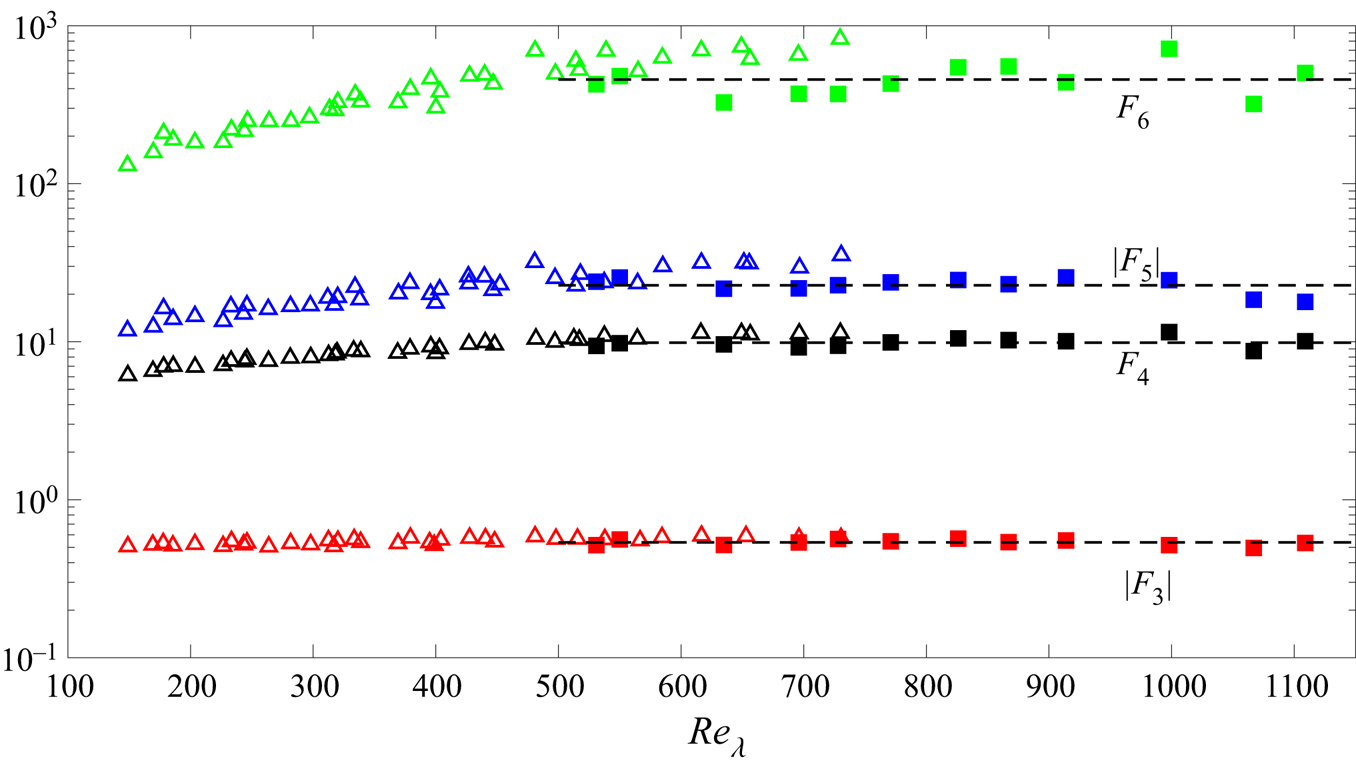
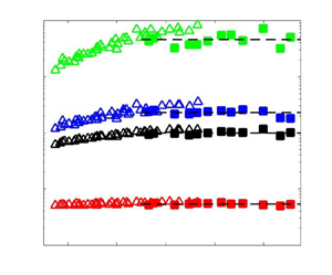
${F_{n + 1}}$ increases with $R{e_\lambda }$, as predicted by K62, or approaches a constant, as predicted by K41, (2.12) indicates clearly that one should not ignore the effect of the large-scale forcing on ${S_{n + 2}}$, ${P_{n + 2}}$ and ${{{G_{n + 2}}}}/{{R{e_\lambda }}}$ before testing the prediction of either K41 or K62. In the context of K41 or K62, for which the power-law exponent for $F_{n + 1}$ (see (1.2)) is smaller than 1, the manner in which ${S_{n + 2}} + {P_{n + 2}} - {{{G_{n + 2}}}}/{{R{e_\lambda }}}$ approaches zero depends on $n$, $F_{n + 1}$ and $m$. The larger $F_{n + 1}$ will result in a slower approach. On the contrary, if ${\alpha _{(n+1)}}$ in (1.2) is larger or equal to 1, the effect of the larger scale forcing on ${S_{n + 2}}$, ${P_{n + 2}}$ and ${{{G_{n + 2}}}}/{{R{e_\lambda }}}$ will never disappear. For shearless grid turbulence, Gylfason, Ayyalasomayajula & Warhaft (Reference Gylfason, Ayyalasomayajula and Warhaft2004) showed that $F_{3}\sim Re_\lambda ^{0.09}$, $F_{4}\sim Re_\lambda ^{0.39}$, $F_{5}\sim Re_\lambda ^{0.63}$ and $F_{6}\sim Re_\lambda ^{1.08}$; note that the data for $F_{4}$ have been reappraised in the context of the finite Reynolds number effect by Tang et al. (Reference Tang, Antonia, Djenidi, Danaila and Zhou2018). These data are shown in figure 1, where a linear scale is used for $Re_\lambda$. Recent results show however that $F_{3}$, $F_{4}$, $F_{5}$ and $F_{6}$ are approximately constant over a significant range of $Re_\lambda$ (${\simeq }500\text {--}1150$) along the axes of a plane jet (Antonia et al. Reference Antonia, Djenidi, Danaila and Tang2017) and a circular jet (Tang et al. Reference Tang, Antonia, Djenidi, Danaila and Zhou2018). The data for the plane jet are included in figure 1 for comparison. This figure suggests that the power-law formulation (1.2) for $F_{3}$, $F_{4}$, $F_{5}$ and $F_{6}$ (K62) mimics reasonably well the finite Reynolds number effect. Thus, altogether, these results indicate that once $Re_\lambda$ becomes sufficiently large, the normalized moments exhibit a plateau. The value of the plateau is approximately 0.54 for $|F_{3}|$ and 10 for $F_{4}$ for both the shearless grid turbulence data of Gylfason et al. (Reference Gylfason, Ayyalasomayajula and Warhaft2004) and the plane jet data for $Re_\lambda \gtrsim 550$. Over the same $Re_\lambda$ range, the values of $|F_{5}|$ and $F_{6}$ may be slightly larger in shearless grid turbulence than on the plane jet axis; the reason for this small difference deserves further investigation.


Dependence of  $|F_{3}|$,
 $F_{4}$,
 $|F_{5}|$ and
 $F_{6}$ on
 $Re_\lambda$ along the axis of the plane jet, reproduced from figure 2 of Antonia et al. (Reference Antonia, Djenidi, Danaila and Tang2017) (
 $\blacksquare$), and in grid turbulence, reproduced from figure 3 of Gylfason et al. (Reference Gylfason, Ayyalasomayajula and Warhaft2004) (
 $\triangle$); for the latter, only the laboratory shearless grid turbulence data are shown. The horizontal dashed lines indicate the mean values of each of the plotted quantities for the plane jet data.

It is generally accepted that LI is satisfied closely in shearless grid turbulence. LI is also satisfied closely on the plane jet axis in the dissipative range, at least in the context of the second- and third-order statistics (Tang et al. Reference Tang, Antonia, Djenidi, Danaila and Zhou2017). In the sense implied by K41 and K62, LI should apply to all statistical moments, not only second- and third-order quantities. As pointed out in § 1, the fourth-order velocity derivative moments can be expressed in terms of four invariants ( $I_1$,
 $I_2$,
 $I_3$ and
 $I_4$) and thus can be used to test LI. However, we follow Siggia (Reference Siggia1981) and use the following four relations
 \begin{equation} \left.\begin{gathered} {D_1} = \overline{{{\left( {\frac{{\partial u}}{{\partial x}}} \right)}^4}} = \frac{{4{I_1}}}{{105}}, \\ {D_2} = \overline{{{\left( {\frac{{\partial u}}{{\partial x}}} \right)}^2}{{\left( {\frac{{\partial v}}{{\partial x}}} \right)}^2}} = \frac{{{I_1}}}{{105}} + \frac{{{I_2}}}{{70}} - \frac{{{I_3}}}{{105}}, \\ {D_3} = \overline{{{\left( {\frac{{\partial v}}{{\partial x}}} \right)}^4}} = \frac{{3{I_1}}}{{140}} + \frac{{11{I_2}}}{{140}} -\frac{{3{I_3}}}{{35}} + \frac{{{I_4}}}{{80}}, \\ {D_4} = \overline{{{\left( {\frac{{\partial u}}{{\partial x}}} \right)}^2}{{\left( {\frac{{\partial v}}{{\partial z}}} \right)}^2}} = \frac{{{I_1}}}{{105}} + \frac{{{I_2}}}{{210}} + \frac{{2{I_3}}}{{105}}, \end{gathered}\right\} \end{equation}
because they can be determined experimentally; here  ${D_1}$,
 ${D_2}$ and
 ${D_3}$ are estimated from the experimental data measured with a one-dimensional vorticity probe in a plane jet (a detailed description is given in Tang et al. Reference Tang, Antonia, Djenidi, Danaila and Zhou2017). If LI is satisfied, then any fourth-order statistical moment can be determined by
 $D_\beta$ (
 $\beta = 1,2,3,4$). Interestingly, Siggia (Reference Siggia1981) pointed out that there is no freedom for different velocity derivatives to scale differently with Reynolds number, i.e.
 ${{{I_\beta }}}/{{{I_1}}}$ must approach a constant as
 $Re_\lambda$ increases. Accordingly,
 ${{{D_\beta }}}/{{{D_1}}}$ must also approach a constant as
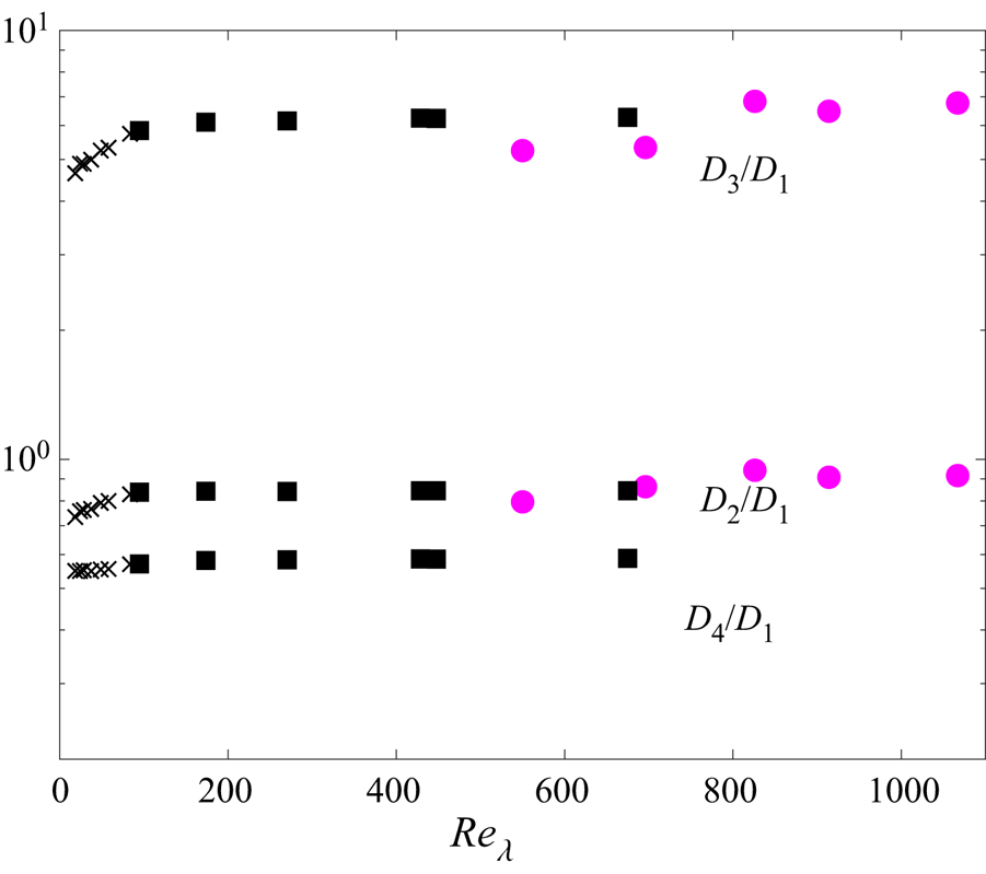
 $Re_\lambda$ increases. Figure 2 shows the ratio
 ${{{D_\beta }}}/{{{D_1}}}$ (
 $\beta = 2,3$) as a function of
 $Re_\lambda$ for the plane jet data. For reference, the ratio with
 $\beta = 2, 3, 4$ for stationary forced periodic box turbulence, where it is generally accepted that LI is closely satisfied (Kerr Reference Kerr1985; Ishihara et al. Reference Ishihara, Kaneda, Yokokawa, Itakura and Uno2007), is also shown. In this latter flow, the ratio
 ${{{D_\beta }}}/{{{D_1}}}$ (
 $\beta = 2,3,4$) becomes
 $Re_\lambda$-independent when
 $Re_\lambda \geq 100$. For the present data, both
 ${{{D_2 }}}/{{{D_1}}}$ and
 ${{{D_3 }}}/{{{D_1}}}$ are approximately constant over the range
 $Re_{\lambda } = 500{\sim}1100$ with almost the same magnitudes as in box turbulence, which indicates that LI is adequately satisfied by the plane jet data.
Variation of  ${{{D_\beta }}}/{{{D_1}}}$ (
 $\beta = 2,3$) with
 $Re_\lambda$ for the plane jet data (
 $\bigcirc$, magenta). For reference, the data for stationary forced periodic box turbulence (
 $\beta = 2,3,4$) are also shown,
 ${\times }$, Kerr (Reference Kerr1985);
 $\blacksquare$, Ishihara et al. (Reference Ishihara, Kaneda, Yokokawa, Itakura and Uno2007) (only the data for
 $k^*_{max}=2$ are shown).

The transport equation for  $\overline \varepsilon$ (
 $= \nu \overline {{{( {{{\partial {u_i}}}/{{\partial {x_k}}}} )}^2}}$), or equivalently the mean enstrophy
 $\overline {{\omega ^2}}$ for homogeneous turbulence, can be obtained from (2.4) by summation of the equations corresponding to all combinations of
 $i$,
 $k$ and
 $j$ for
 $n=1$. The resulting equation is
 \begin{equation} \frac{1}{{2\nu}}{U_1}\frac{\partial }{{\partial {x_1}}}\overline \varepsilon + \overline{\left( {\frac{{\partial {u_i}}}{{\partial {x_k}}}} \right)\frac{{\partial {u_j}}}{{\partial {x_k}}} \frac{{\partial {u_i}}}{{\partial {x_j}}}} + \overline{\left( {\frac{{\partial {u_i}}}{{\partial {x_k}}}} \right) \frac{\partial }{{\partial {x_k}}}\frac{{\partial p}}{{\partial {x_i}}}} - \nu \overline{\left( {\frac{{\partial {u_i}}}{{\partial {x_k}}}} \right)\frac{\partial }{{\partial {x_k}}} \frac{\partial }{{\partial {x_j}}}\frac{{\partial {u_i}}}{{\partial {x_j}}}} = 0, \end{equation}
where the repeated indices  $i$,
 $j$ and
 $k$ indicate summation. The pressure term can be rewritten as
 \begin{equation} {\overline{\left( {\frac{{\partial {u_i}}}{{\partial {x_k}}}} \right)\frac{\partial }{{\partial {x_k}}} \frac{{\partial p}}{{\partial {x_i}}}} = \frac{\partial }{{\partial {x_i}}} \overline{\left( {\frac{{\partial {u_i}}}{{\partial {x_k}}}} \right)\frac{{\partial p}}{{\partial {x_k}}}} - \overline{\frac{{\partial p}}{{\partial {x_k}}}\frac{\partial }{{\partial {x_k}}} \left( {\frac{{\partial {u_i}}}{{\partial {x_i}}}} \right)} } \end{equation}
and is zero owing to homogeneity ( ${({\partial }/{{\partial {x_i}}})\overline {( {} )} = 0}$) and incompressibility (
 ${{{\partial {u_i}}}/{{\partial {x_i}}}}=0$). Equation (2.15) then reduces to the well-known equation originally obtained by Batchelor & Townsend (Reference Batchelor and Townsend1947) and which expresses the balance between the production of
 $\overline {{{({{{\partial {u_i}}}/{{\partial {x_k}}}} )}^2}}$ through vortex stretching and its destruction through viscous action. When LI is assumed, this equation simplifies to
 \begin{equation} \frac{1}{{35\nu }}{U_1}\frac{{\partial \bar \varepsilon }}{{\partial {x_1}}} + \overline{{{\left( {\frac{{\partial {u_1}}}{{\partial {x_1}}}} \right)}^3}} + 2\nu \overline{{{\left( {\frac{{{\partial ^2}{u_1}}}{{\partial x_1^2}}} \right)}^2}} = 0. \end{equation}
There are three combinations ( $i=k=1$,
 $i=2$
 $k=1$,
 $i=3$
 $k=1$), (
 $i=1$
 $k=2$,
 $i=k=2$,
 $i=3$
 $k=2$), (
 $i=1$
 $k=3$,
 $i=2$
 $k=3$,
 $i=k=3$) for which the pressure-strain rate term disappears (e.g. Vreman & Kuerten Reference Vreman and Kuerten2014). It is important to note however that for any specific combinations of
 $i$ and
 $k$, the pressure-strain rate term may not be immediately neglected. If LI is assumed, this term can, e.g. by similarity to the fourth-order-tensorial expression given by Antonia & Browne (Reference Antonia and Browne1983) with
 $p$ replacing
 $\theta$ (a passive temperature fluctuation), be written as
 \begin{equation} \overline{\frac{{\partial p}}{{\partial {x_l}}}\frac{\partial }{{\partial {x_k}}} \left( {\frac{{\partial {u_i}}}{{\partial {x_j}}}} \right)} = b\left( {{\delta _{ik}}{\delta _{jl}} + {\delta _{il}}{\delta _{jk}} - \frac{2}{3}{\delta _{ij}}{\delta _{kl}}} \right), \end{equation}
where  $b$ is constant. It follows, for example for
 $k=l=1$, that
 \begin{equation} \overline{\frac{{\partial p}}{{\partial {x_1}}}\frac{\partial }{{\partial {x_1}}} \left( {\frac{{\partial {u_1}}}{{\partial {x_1}}}} \right)} = \frac{4}{3}b, \end{equation}
when  $i=j=1$ or
 \begin{equation} \overline{\frac{{\partial p}}{{\partial {x_1}}}\frac{\partial }{{\partial {x_1}}} \left( {\frac{{\partial {u_2}}}{{\partial {x_2}}}} \right)} = \overline{\frac{{\partial p}}{{\partial {x_1}}} \frac{\partial }{{\partial {x_1}}}\left( {\frac{{\partial {u_3}}}{{\partial {x_3}}}} \right)} ={-} \frac{2}{3}b, \end{equation}
when  $i=j=2$ or 3. When LI is assumed, (2.4) for
 $n=1$ and any combination of
 $i$ and
 $k$ will simplify to an expression which can be reconciled with (2.17) only when
 $b=0$. One may expect that
 $b \ne 0$ for finite
 ${Re_\lambda }$. The magnitude of
 $b$ should however decrease as
 ${Re_\lambda }$ increases and thus lead to the isotropization of the small-scale turbulence.
3. Transport equations for the normalized odd moments of the transverse velocity derivative ${F_{y,3}}$, ${F_{y,5}}$ and ${F_{y,7}}$ in shearless and sheared grid turbulence


We now focus on the transport equations for the normalized odd moments of the transverse velocity derivative, which can be obtained from (2.4) by taking  $i=1$ and
 $k=2$, i.e.
 \begin{align} & \frac{1}{{n + 1}}{{U}_1}\frac{\partial }{{\partial {x_1}}} \overline{{{\left( {\frac{{\partial {u_1}}}{{\partial {x_2}}}} \right)}^{n + 1}}} + \overline{{{\left( {\frac{{\partial {u_1}}}{{\partial {x_2}}}} \right)}^n} \frac{{\partial {u_j}}}{{\partial {x_2}}}\frac{{\partial {u_1}}}{{\partial {x_j}}}} \nonumber\\ &\quad + \overline{{{\left( {\frac{{\partial {u_1}}}{{\partial {x_2}}}} \right)}^n} \frac{\partial }{{\partial {x_2}}}\frac{{\partial p}}{{\partial {x_1}}}} - \nu \overline{{{\left( {\frac{{\partial {u_1}}}{{\partial {x_2}}}} \right)}^n}\frac{\partial }{{\partial {x_2}}} \frac{\partial }{{\partial {x_j}}}\frac{{\partial {u_1}}}{{\partial {x_j}}}} = 0. \end{align}
To arrive at (3.1), we used the following approximations:
 \begin{equation} \left| {\frac{1}{{n + 1}}\frac{\partial }{{\partial {x_1}}} \overline{{u_1}{{\left( {\frac{{\partial {u_1}}}{{\partial {x_2}}}} \right)}^{n + 1}}} } \right| \ll \left| {\frac{{{U_1}}}{{n + 1}}\overline{\frac{\partial }{{\partial {x_1}}}{{\left( {\frac{{\partial {u_1}}}{{\partial {x_2}}}} \right)}^{n + 1}}} } \right| \end{equation}
and
 \begin{equation} \left| {\overline{{{\left( {\frac{{\partial {u_1}}}{{\partial {x_2}}}} \right)}^n}} \frac{\partial }{{\partial {x_1}}}\frac{{\partial \overline{{u_1}{u_1}} }}{{\partial {x_1}}}} \right| \ll \left| {\overline{{{\left( {\frac{{\partial {u_1}}}{{\partial {x_2}}}} \right)}^n} \frac{{\partial {u_j}}}{{\partial {x_2}}}\frac{{\partial {u_1}}}{{\partial {x_j}}}} } \right|. \end{equation}
These two assumptions are discussed and justified in Appendix B for shearless and sheared grid turbulence. After normalizing by  $\overline {{{( {\partial {u_1}/\partial {x_1}} )}^2}}$, (3.1) becomes
 \begin{equation} - \frac{1}{{n + 1}}{{U}_1}\frac{\partial }{{\partial {x_1}}} \overline{{{\left( {\frac{{\partial {u_1}}}{{\partial {x_2}}}} \right)}^{n + 1}}} = {\overline{{{\left( {\frac{{\partial {u_1}}}{{\partial {x_1}}}} \right)}^2}} ^{(n + 2)/2}} \left[ {{S_{y,n + 2}} + {P_{y,n + 2}} - \frac{{{G_{y,n + 2}}}}{{R{e_\lambda }}}} \right], \end{equation}
where  ${S_{y,n + 2}}$,
 ${P_{y,n + 2}}$ and
 ${G_{y,n + 2}}$, like
 ${S_{n + 2}}$,
 ${P_{n + 2}}$ and
 ${G_{n + 2}}$, are small-scale quantities, defined as
 \begin{gather} {S_{y,n + 2}} = \frac{{\overline{{{\left( {\dfrac{{\partial {u_1}}}{{\partial {x_2}}}} \right)}^n} \dfrac{{\partial {u_j}}}{{\partial {x_2}}}\dfrac{{\partial {u_1}}}{{\partial {x_j}}}} }}{{{{\overline{{{\left( {\dfrac{{\partial {u_1}}}{{\partial {x_1}}}} \right)}^2}} }^{(n + 2)/2}}}}, \end{gather}
 \begin{gather}{P_{y,n + 2}} = \frac{{\overline{{{\left( {\dfrac{{\partial {u_1}}}{{\partial {x_2}}}} \right)}^n}\dfrac{\partial }{{\partial {x_2}}}\dfrac{{\partial p}}{{\partial {x_1}}}} }}{{{{\overline{{{\left( {\dfrac{{\partial {u_1}}}{{\partial {x_1}}}} \right)}^2}} }^{(n + 2)/2}}}}, \end{gather}
 \begin{gather}{G_{y,n + 2}} = \frac{{\overline{u_1^2} \overline{{{\left( {\dfrac{{\partial {u_1}}}{{\partial {x_2}}}} \right)}^n}\dfrac{{{\partial ^3}{u_1}}}{{\partial {x_2}\partial {x_j}\partial {x_j}}}} }}{{{{\overline{{{\left( {\dfrac{{\partial {u_1}}}{{\partial {x_1}}}} \right)}^2}} }^{(n + 3)/2}}}}. \end{gather}
If one assumes  $\overline {{u_1^2}}\sim x_1^{m }$, then (3.4) reduces to
 \begin{equation} \frac{{{C_{y,n + 2}}}}{{R{e_\lambda }}} = {S_{y,n + 2}} + {P_{y,n + 2}} - \frac{{{G_{y,n + 2}}}}{{R{e_\lambda }}}, \end{equation}
where
 \begin{equation} {C_{y,n + 2}} = \frac{{5( - m + 1){F_{y,n + 1}}}{{R_s^{-(n + 1)/2}}}}{-m}, \end{equation}
where
 \begin{equation} R_s = \frac{{\overline{{{\left( {\dfrac{{\partial {u_1}}}{{\partial {x_1}}}} \right)}^2}} }}{{\overline{{{\left( {\dfrac{{\partial {u_1}}}{{\partial {x_2}}}} \right)}^2}} }}. \end{equation}
The derivations of (3.4) to (3.8) are shown in Appendix D for shearless grid turbulence. Taking  $i=1$ and
 $k=3$ in (2.4) and repeating the above procedure, we can obtain the transport equations for the normalized moments of the transverse velocity derivative in the
 $x_3$ direction, i.e.
 \begin{equation} {F_{z,n + 1}} = \frac{{\overline{{{\left( {\dfrac{{\partial {u_1}}}{{\partial {x_3}}}} \right)}^{n + 1}}} }}{{{{\overline{{{\left( {\dfrac{{\partial {u_1}}}{{\partial {x_3}}}} \right)}^2}} }^{(n + 1)/2}}}}. \end{equation}
Further, by choosing  $n=1,3, 5,\ldots$ in (3.8), we can also obtain the transport equations for the normalized even moments of the transverse velocity derivative. Similar comments to those associated with (2.12) can be made and are therefore not repeated here. Finally, taking
 $n=2, 4, 6$, (3.8) leads to the transport equations for the normalized odd moments of the transverse velocity derivative
 ${F_{y,3}}$,
 ${F_{y,5}}$ and
 ${F_{y,7}}$. Note that for
 $n=2, 4, 6$ and when LI is satisfied, any combination of the indices in
 ${S_{y,n + 2}}$,
 ${P_{y,n + 2}}$ and
 ${G_{y,n + 2}}$ will lead to a term involving the Kronecker delta
 $\delta _{12}$, which is zero. To simplify the analysis, we rewrite (3.8) as
 \begin{equation} \frac{{{C_{y,n + 2}}}}{{R{e_\lambda }}} =SPG_{y,n + 2}, \end{equation}
where  $SPG_{y,n + 2}= {S_{y,n + 2}} + {P_{y,n + 2}} - {{{G_{y,n + 2}}}}/{{R{e_\lambda }}}$ (
 $n=2, 4, 6$) should be zero if LI is satisfied. The parameters
 $R_s$ and
 ${F_{y,n+1}}$ (
 $n=2, 4, 6$), which should be 0.5 and 0 under LI, represent a measure of small-scale anisotropy. Because the derivation of (3.12) does not assume LI, then
 $R_s$ and
 ${F_{y,n+1}}$ can be used to quantify how the departure from LI (i.e.
 ${F_{y,n+1}}\ne 0$ and
 $R_s\ne 0.5$) affects
 $SPG_{y,n + 2}$. Although
 $R_s$ is nearly 0.5 in shearless grid turbulence (e.g. Danaila et al. Reference Danaila, Zhou, Anselmet and Antonia2000), there is a large scatter for
 $R_s$ in sheared grid turbulence. For example, Tavoularis & Corrsin (Reference Tavoularis and Corrsin1981a,Reference Tavoularis and Corrsinb) found that
 $R_s\approx 0.2$ at
 $Re_\lambda =160$ but
 $R_s\approx 0.5$ for
 $Re_\lambda =140\text {--}660$ in the experiment of Ferchichi & Tavoularis (Reference Ferchichi and Tavoularis2000). It is possible that this difference in
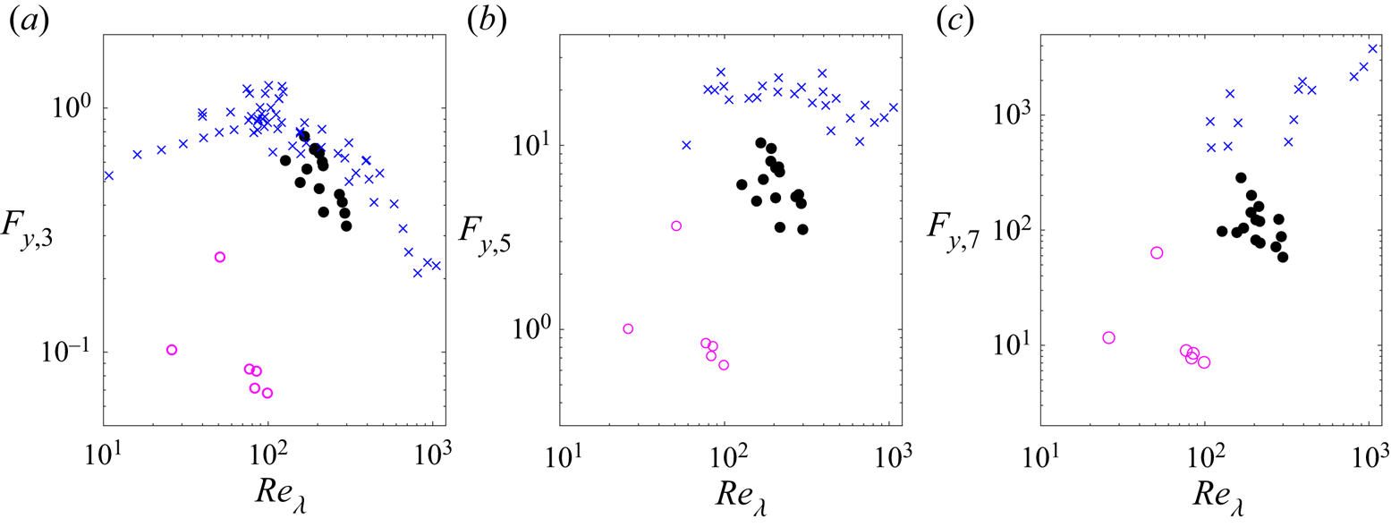
 $R_s$ reflects differences in the initial conditions between the two experiments. Figure 3 shows the distributions of
 ${F_{z,3}}$,
 ${F_{z,5}}$ and
 ${F_{z,7}}$ on the axis of the intermediate wakes generated using five different initial conditions (a solid circular cylinder, a solid square cylinder, a screen circular cylinder, a solid plate and screen strip), and the distributions of
 ${F_{y,3}}$,
 ${F_{y,5}}$ and
 ${F_{y,7}}$ in sheared grid turbulence and shearless grid turbulence.
(a–c) Dependence of  ${F_{y,3}}$,
 ${F_{y,5}}$ and
 ${F_{y,7}}$ on
 $Re_\lambda$ in sheared and shearless grid turbulence. The data for sheared grid turbulence (
 $\times$, blue) are reproduced from Schumacher et al. (Reference Schumacher, Sreenivasan and Yeung2003) and Shen & Warhaft (Reference Shen and Warhaft2000) without identifying the sources. The data for shearless grid turbulence (
 $\bigcirc$, magenta) are calculated from the data of Zhou & Antonia (Reference Zhou and Antonia2000b). For comparison, the data for
 ${F_{z,3}}$,
 ${F_{z,5}}$ and
 ${F_{z,7}}$ (
 $\bigcirc$, black) in intermediate wakes, generated using several different initial conditions, are also shown (Tang et al. Reference Tang, Antonia, Danaila, Djenidi, Zhou and Zhou2016).

Some remarks are warranted before discussing figure 3. Although (3.12) is derived for shearless grid turbulence, it should also apply to the centreline of the intermediate wake of solid circular cylinder because the one-point energy budget in this flow region (Thiesset, Antonia & Danaila Reference Thiesset, Antonia and Danaila2013) is similar to that for shearless grid turbulence. In sheared grid turbulence, the one-point energy budget can be approximated by
 \begin{equation} \bar \varepsilon ={-} \frac{1}{2}U_1\frac{{\partial \overline{{u_i^2}} }}{{\partial x_1}} - \overline{u_1u_2} \frac{{\partial U_1}}{{\partial x_2}}.\end{equation}
If there is no advection term, i.e.  $\bar \varepsilon \approx - \overline {u_1u_2} ({{\partial U_1}}/{{\partial x_2}})$ or
 $- \frac {1}{2}U_1({{\partial \overline {{u_i^2}} }}/{{\partial x_1}})\approx 0$ in sheared grid turbulence, the flow is not decaying and thus the term on the left-hand side of (3.12) (or equivalently
 ${{{C_{y,n + 2}}}}/{{R{e_\lambda }}}$ in (3.12)) should be negligible. In this situation, non-zero values of
 ${F_{y,3}}$,
 ${F_{y,5}}$ and
 ${F_{y,7}}$ will not directly affect small-scale quantities
 $SPG_{y,n + 2}$ and the production term should have a significant effect on small-scale quantities; the latter will be discussed in some detail in the next section. However, the experiments of Ferchichi & Tavoularis (Reference Ferchichi and Tavoularis2000) and Shen & Warhaft (Reference Shen and Warhaft2000) indicated that the ratio
 $-\overline {u_1u_2} ({{\partial U_1}}/{{\partial x_2}})/\bar \varepsilon _{iso}$ is approximately 1.51 and 1.81 at
 $Re_\lambda =972$ and 204, respectively. Namely, the contribution from the advection term to the one-point energy budget cannot be discounted. To quantify how the departure from LI (i.e.
 ${F_{y,n+1}}\ne 0$) affects the small-scale quantities in sheared grid turbulence, we assume that the production and advection are proportional to each other and thus we write
 \begin{equation} \overline{{u_1}{u_2}} \frac{{\partial {U_1}}}{{\partial {x_2}}} = A\frac{1}{2}{U_1} \frac{{\partial \overline{{q^2}} }}{{\partial {x_1}}}, \end{equation}
where  $A$ is a constant depending on the particular experiment or simulation and
 $\overline {q^2}=\overline {u_i^2}$. Therefore, (3.13) can be written as
 \begin{equation} \bar \varepsilon ={-} (A+1)\frac{1}{2}U_1\frac{{\partial \overline{{{q^2}}} }}{{\partial x_1}}. \end{equation}
The purpose of introducing (3.14) is to obtain a power-law decay rate for  $\overline \varepsilon$ using (3.15) after assuming a power-law decay rate for
 $\overline {{q^2}} \sim x_1^{m_1}$ in sheared grid turbulence, where
 $m_1$ may differ from
 $m$. This will allow the large-scale term in (3.4) to be simplified significantly, which will be discussed in the context of (3.18). We recall that LI is generally not satisfied in this flow. Therefore, to avoid the ambiguity arising from the directional dependence of
 $\overline {{u_1^2}}$ and
 $\lambda$ used to define
 $Re_\lambda$, we adopt here a more general definition, i.e.
 \begin{equation} Re_{\lambda_{q}} = \frac{{{{\overline{{q^2}} }^{1/2}}}}{{{3^{1/2}}}}\frac{{{\lambda _q}}}{\nu}, \end{equation}
where  $\lambda _q$ is given by
 \begin{equation} {\lambda _q} = {(5\nu )^{1/2}}\frac{{{{\overline{{q^2}} }^{1/2}}}}{{{{\overline \varepsilon }^{1/2}}}}. \end{equation}
The definition of  $Re_\lambda$ is equivalent to that of
 $Re_{\lambda _{q}}$ only when isotropy applies (at all scales), i.e.
 $\overline {{q^2}} =3\overline {{u_1^2}}$ and
 $\overline \varepsilon =\overline \varepsilon _{iso}=15\nu \overline {{{({\partial {u_1}/\partial {x_1}})}^2}}$. Using the power-law decay rate
 $\overline {{q^2}} \sim x_1^{m_1}$ and definition of
 $Re_{\lambda _{q}}$ (3.16) and (3.15), the large-scale term in (3.4) leads to
 \begin{align} & {{-\frac{1}{{n +
1}}{U_1}\frac{\partial }{{\partial {x_1}}}
\overline{{{\left( {\frac{{\partial {u_1}}}{{\partial
{x_2}}}} \right)}^{n + 1}}} }\biggl/{{{\overline{{{\left(
{\frac{{\partial {u_1}}}{{\partial {x_1}}}} \right)}^2}}
}^{(n + 2)/2}}}} \nonumber\\ &\quad = \frac{{{F_{y,n +
1}}R_s^{{ - (n + 1)/2}}(1 - {m_1})5\sqrt {{R_{iso}}} }}{{(
- {m_1})(A + 1){Re_{{\lambda _q}}}}} = \frac{{{C_{y0,n +
2}}\sqrt {{R_{iso}}} }}{{(A + 1){Re_{{\lambda _q}}}}},
\end{align}
where
 \begin{equation} {C_{y0,n + 2}} = \frac{{5( - m_1 + 1){F_{y,n + 1}}}{{R_s^{-(n + 1)/2}}}}{-m_1}, \end{equation}
and  $R_{iso}=\overline \varepsilon _{iso} /\overline \varepsilon$, which represents a measure of small-scale anisotropy. The detailed derivation is shown in Appendix D in sheared grid turbulence. It can be observed from (3.18) and (3.12) that the advection of
 ${F_{y,n + 1}}$ by
 $U_1$ can be recast in the same manner in both shearless and sheared grid turbulence. Actually, if one focuses on shearless grid turbulence under the the assumption of isotropy,
 $m_1=m$ (
 ${C_{y0,n + 2}}$ will be equal to
 ${C_{y,n + 2}}$ in (3.9)),
 $R_{iso}=1$,
 $Re_{\lambda _{q}}=Re_\lambda$ and
 $A=0$ (the production term in (3.14) disappears so (3.18) will become identical to the left-hand side of (3.12).
The following comments can be made with regard to figure 3, (3.12) and (3.18).
(i) It is clear that the magnitude of the normalized odd moments of the transverse velocity derivative differs from flow to flow for all the flows considered here. Its value is largest for sheared grid turbulence followed by the centreline of the intermediate wake, then the shearless grid turbulence.
(ii) None of the values in figure 3 are zero, which underlines the absence of local isotropy, even in shearless grid turbulence. With the exception of
${F_{y,5}}$ and ${F_{y,7}}$ in sheared grid turbulence, the other quantities decrease as $Re_{\lambda }$ increases, which is consistent with the idea that the small scales approach LI with increasing $Re_\lambda$. However, in sheared grid turbulence, ${F_{y,5}}$ does not diminish perceptibly even when $Re_\lambda$ is as high as 1000 and ${F_{y,7}}$ even increases with $Re_\lambda$ (Shen & Warhaft (Reference Shen and Warhaft2000) showed ${F_{y,7}} \sim Re_\lambda ^{0.63}$).(iii) Although, these results, especially those for sheared grid turbulence, have been interpreted as implying that the small-scale anisotropy can persist to very high Reynolds numbers, the transport equations for the normalized odd moments, i.e. (3.8) (or (3.18)) for
$n=2, 4, 6$, imply that the departure from LI, as reflected by the non-zero values of ${F_{y,3}}$, ${F_{y,5}}$ and ${F_{y,7}}$, will not affect small-scale quantities $SPG_{y,n + 2}$ when $Re_\lambda$ (or $Re_{\lambda _{q}}$) is sufficiently large. Larger ${F_{y,3}}$, ${F_{y,5}}$ and ${F_{y,7}}$ values will lead to a slower rate at which this effect will disappear.(iv) The small-scale anisotropy persists to Reynolds numbers as high as
$Re_\lambda \sim 1000$. This implies that effects of the large-scale inhomogeneity on the small scales are still non-negligible suggesting that the value 1000 should not be considered as ‘sufficiently large’ for ignoring the large-scale anisotropy effect. As an example, let us estimate $SPG_{y,8}$, which is zero when LI is satisfied. To do this, we use the value of ${F_{y,7}}$ at the largest $Re_\lambda$ in figure 3(c) (${F_{y,7}}=3772$ at $Re_\lambda =1054$) and $R_s\approx 0.5$ for $Re_\lambda =140\text {--}660$ in the experiment of Ferchichi & Tavoularis (Reference Ferchichi and Tavoularis2000). This yields
(3.20)Note that, for this estimation,\begin{align} SP{G_{y,8}} = \frac{{{C_{y,n + 2}}}}{{R{e_\lambda }}} = \frac{{\dfrac{{5( - {m_1} + 1){F_{y,n + 1}}R_s^{ - (n + 1)/2}}}{{ - {m_1}}}}}{{R{e_\lambda }}} > \frac{{5{F_{y,n + 1}}R_s^{ - 7/2}}}{{R{e_\lambda }}} = 202. \end{align}${{( - {m_1} + 1)}}/{{ - {m_1}}}$ has been assumed to be larger than 1. Clearly, $SP{G_{y,8}}$ is far from zero, which indicates a departure from LI. It is however evident that $SP{G_{y,8}}$ will decrease as $Re_\lambda$ increases.


4. Effect of the mean shear
As shown in figure 3, the mean shear appears to have a non-negligible effect on  ${F_{y,3}}$,
 ${F_{y,5}}$ and
 ${F_{y,7}}$. However, does the mean shear directly affect small-scale quantities such as
 ${S_{n + 2}}$,
 ${P_{n + 2}}$ and
 ${G_{n + 2}}$ in (2.12)? To address this issue, we now focus our attention on sheared grid turbulence with a mean velocity gradient in the
 $x_2$ direction (
 ${{\partial {{U}_1}}}/{{\partial {x_2}}}$). We first assume that the term in (2.2) associated with
 ${{\partial {{U}_1}}}/{{\partial {x_2}}}$, i.e. the second term on the second line of (2.2), is the dominant (large-scale) term. Taking
 $i=k=1$, this term becomes, after some trivial manipulations,
 \begin{equation}
\left.\begin{gathered}
\hspace{-12pc}\frac{{\overline{{{\left( {\dfrac{{\partial
{u_1}}}{{\partial {x_1}}}} \right)}^n} \dfrac{{\partial
{u_2}}}{{\partial {x_1}}}} \dfrac{{\partial
{{U}_1}}}{{\partial {x_2}}}}}{{{{\overline{{{\left(
{\dfrac{{\partial {u_1}}}{{\partial {x_1}}}} \right)}^2}}
}^{(n + 2)/2}}}} = \frac{{\overline{{{\left(
{\dfrac{{\partial {u_1}}}{{\partial {x_1}}}} \right)}^n}
\dfrac{{\partial {u_2}}}{{\partial {x_1}}}}
\dfrac{{\partial {{U}_1}}}{{\partial
{x_2}}}}}{{{{\overline{{{\left( {\dfrac{{\partial
{u_1}}}{{\partial {x_1}}}} \right)}^2}} }^{(n +
1)/2}}{{\overline{{{\left( {\dfrac{{\partial
{u_1}}}{{\partial {x_1}}}} \right)}^2}} }^{1/2}}}} \\ =
\frac{{15\nu \overline{{{\left( {\dfrac{{\partial
{u_1}}}{{\partial {x_1}}}} \right)}^n} \dfrac{{\partial
{u_2}}}{{\partial {x_1}}}} \overline{u_1^2}
\dfrac{{\partial {{U}_1}}}{{\partial
{x_2}}}{{\overline{{{\left( {\dfrac{{\partial
{u_1}}}{{\partial {x_1}}}} \right)}^2}} }^{1/2}}}}{{15\nu
{{\overline{{{\left( {\dfrac{{\partial {u_1}}}{{\partial
{x_1}}}} \right)}^2}} }^{(n + 1)/2}}\overline{u_1^2}
\overline{{{\left( {\dfrac{{\partial {u_1}}}{{\partial
{x_1}}}} \right)}^2}} }} = \frac{{15\nu {S_{y,n +
1}}\overline{u_1^2}\dfrac{{\partial {{U}_1}}}{{\partial
{x_2}}}{{\overline{{{\left( {\dfrac{{\partial
{u_1}}}{{\partial {x_1}}}} \right)}^2}} }^{1/2}}}}{{\bar
\varepsilon_{iso} \overline{u_1^2} }} \\ \frac{{15{S_{y,n +
1}}\overline{u_1^2} \dfrac{{\partial {{U}_1}}}{{\partial
{x_2}}}}}{{\bar \varepsilon_{iso} R{e_\lambda }}} =
\frac{{15{S_{s,n + 1}}{S^*}}}{{R{e_\lambda }}}=
\frac{{{C_{s,n + 2}}}}{{R{e_\lambda }}},
\end{gathered}\right\}
\end{equation}
where  ${C_{s,n + 2}}$ is a constant, defined as
 \begin{equation} {C_{s,n + 2}} = 15{S_{s,n + 1}}{S^*}; \end{equation}
 $S^*$ is the non-dimensional shear parameter
 \begin{equation} {S^*} = \frac{{\overline{u_1^2} \dfrac{{\partial {{U}_1}}}{{\partial {x_2}}}}}{{\bar \varepsilon_{iso} }}, \end{equation}
and  ${S_{s,n + 1}}$ is the normalized correlation involving the streamwise derivative of
 $u_1$ and
 $u_2$, defined as
 \begin{equation} {S_{s,n + 1}} = \frac{{\overline{{{\left( {\dfrac{{\partial {u_1}}}{{\partial {x_1}}}} \right)}^n} \dfrac{{\partial {u_2}}}{{\partial {x_1}}}} }}{{{{\overline{{{\left( {\dfrac{{\partial {u_1}}}{{\partial {x_1}}}} \right)}^2}} }^{(n + 1)/2}}}}. \end{equation}
Note that the small-scale quantities  ${S_{n + 2}}$,
 ${P_{n + 2}}$ and
 ${G_{n + 2}}$ are the same as in (2.12). However, studying the effect of the mean shear on other small-scale quantities simply requires changing
 $i$ and
 $k$ independently in (2.2). This is not done here. The dimensional analysis of Schumacher et al. (Reference Schumacher, Sreenivasan and Yeung2003) shows that, if
 $S^*/Re_\lambda \gg 1/8$, the effects of mean shear on small scales will always be felt no matter how high the Reynolds number is. However, (4.2) shows that both
 ${S_{s,n + 1}}$ and
 $S^*$ can affect small-scale quantities. Although the effect of
 $S^*$ has received significant attention for sheared grid turbulence (Schumacher et al. Reference Schumacher, Sreenivasan and Yeung2003), the possible influence of
 ${S_{s,n + 1}}$ on small-scale quantities has largely been ignored in the literature. Note that
 ${S_{s,n + 1}}$ should be zero if LI is satisfied. Even if
 $S^*/Re_\lambda \gg 1/8$, once
 $15{S_{s,n + 1}}{S^*}/Re_\lambda$ is small compared with
 ${S_{n + 2}}$ at given
 $n$ when
 $Re_\lambda$ is sufficiently large, the effect of the mean shear on small scales can be negligible. More importantly, the larger the product
 ${S_{s,n + 1}}{S^*}$, the slower the rate at which this effect will disappear. The difference between the present results and those of Schumacher et al. (Reference Schumacher, Sreenivasan and Yeung2003) is not surprising because the present inference from the N–S equations should be superior to a conclusion based on dimensional arguments.
5. Conclusions and discussions
The transport equations for the normalized  $n^{th}$-order moments of velocity derivatives are derived from the N–S equations for sheared and shearless grid turbulence. The particular critical feature of these equations is that they do not assume local isotropy, thus providing an ideal framework for assessing the effect of large-scale forcing (or inhomogeneity) arising from the advection and production terms on small-scale turbulence. The major conclusions can be summarized as follows.
(1) For shearless grid turbulence, the influence of the (large-scale) streamwise advection of
${F_{n + 1}}$ by the mean velocity on the normalized moments of the velocity derivatives can be expressed in the form $C_1 F_{n + 1}/Re_\lambda$. Accordingly, regardless of whether the variation of ${F_{n + 1}}$ with $Re_\lambda$ follows K41 or K62, for which the power-law exponent for $F_{n + 1}$ ($|F_{n+1}|\sim {Re_\lambda ^{\alpha _{(n+1)}}}$) is smaller than 1, the effect of large scales on small scales will become negligible when $Re_\lambda$ is sufficiently large. The manner in which $C_1 F_{n + 1}/Re_\lambda$ reaches zero depends on the values of $n$, $F_{n + 1}$ and the turbulent energy decay exponent $m$. However, if ${\alpha _{(n+1)}}$ is larger or equal to 1, the effect of the large scales on the small-scale quantities ${S_{n + 2}}$, ${P_{n + 2}}$ and ${{{G_{n + 2}}}}/{{R{e_\lambda }}}$ will increase with $Re_\lambda$.(2) The large-scale effect associated with the streamwise advection of
${F_{y,3}}$, ${F_{y,5}}$ and ${F_{y,7}}$ on $SPG_{y,n + 2}$ ($n=2, 4, 6$), which should be zero if LI is satisfied, can be expressed in the form $C_2 F_{y,n + 1}/Re_\lambda$ for both shearless and sheared grid turbulence. None of the values for ${F_{y,3}}$, ${F_{y,5}}$ and ${F_{y,7}}$ are zero, which underlines the absence of local isotropy. Further, the equations clearly reveal that the departure from local isotropy persists when $Re_\lambda$ is large. Indeed, the available data show that the maximum power-law exponents for ${F_{y,3}}$, ${F_{y,5}}$ and ${F_{y,7}}$ are smaller than 1 (e.g. Shen & Warhaft Reference Shen and Warhaft2000). Larger ${F_{y,3}}$, ${F_{y,5}}$ and ${F_{y,7}}$ values will lead to a slower rate at which local isotropy is approached in the context of $SPG_{y,n + 2}$ for $n=2, 4, 6$ as the Reynolds number increases.(3) The effect of the mean shear on
${S_{n + 2}}$, ${P_{n + 2}}$ and ${G_{n + 2}}$ can be expressed in the form $15{S_{s,n + 1}}{S^*}/Re_\lambda$. Thus, if $15{S_{s,n + 1}}{S^*}/Re_\lambda$ does not increase faster than $Re_\lambda$, its effect on small scales can be negligible (i.e. $15{S_{s,n + 1}}{S^*}/Re_\lambda$ is small compared with ${S_{n + 2}}$ at given $n$) when $Re_\lambda$ is sufficiently large. The larger product ${S_{s,n + 1}}{S^*}$ will result in a slower rate at which this large-scale effect becomes negligible as the Reynolds number increases.


The transport equations developed in this paper represent an important set of constraints for finite-Reynolds-number turbulent flows. They also show how the effect of the large-scale forcing (or inhomogeneity) on small-scale turbulence gradually decreases as the Reynolds number increases and eventually becomes negligible when  $Re_\lambda$ becomes sufficiently large. Finally, we should stress that the large-scale forcing (or inhomogeneity) arising from the advection and production will not vanish even at very large
 $Re_\lambda$. Instead, their contributions will become negligible when
 $Re_\lambda$ is sufficiently large.
Funding
S.L.T wishes to acknowledge support given to him from NSFC through grants 11702074 and 91952109 and from Natural Scientific Research Innovation Foundation in Harbin Institute of Technology through grant HIT.NSRIF.2020059.
Declaration of interests
The authors report no conflict of interest.
Appendix A. Discussion of the approximations in (2.6) and (2.7) in shearless grid turbulence
Equation (2.6),
 \begin{equation} \left| {\frac{1}{{n + 1}}\frac{\partial }{{\partial {x_1}}} \overline{{u_1}{{\left( {\frac{{\partial {u_1}}}{{\partial {x_1}}}} \right)}^{n + 1}}} } \right| \ll \left| {\frac{1}{{n + 1}}\overline{\frac{\partial }{{\partial {x_1}}}{U_1}{{\left( {\frac{{\partial {u_1}}}{{\partial {x_1}}}} \right)}^{n + 1}}}} \right|, \end{equation}
requires only  ${u_1'} \ll {U_1}$ (or equivalently
 ${u_1'}/{U_1} \ll 1$) to be satisfied. This is supported reasonably well by the available shearless grid turbulence data in the literature. For example, Shen & Warhaft (Reference Shen and Warhaft2002) and Gylfason et al. (Reference Gylfason, Ayyalasomayajula and Warhaft2004) showed that
 ${u_1'}/{U_1} <18.1\,\%$ over a significant range of
 $Re_\lambda$ (
 $=$ 26–863) in the shearless grid turbulence. Namely, the assumption in (2.6) is tenable.
Equation (2.7) can be rewritten as
 \begin{align} \left| {\overline{{{\left( {\frac{{\partial {u_1}}}{{\partial {x_1}}}} \right)}^n}} \frac{\partial }{{\partial {x_1}}}\frac{{\partial \overline{{u_1}{u_1}} }}{{\partial {x_1}}}} \right| \ll \left| {\overline{{{\left( {\frac{{\partial {u_1}}}{{\partial {x_1}}}} \right)}^n} \frac{{\partial {u_j}}}{{\partial {x_1}}}\frac{{\partial {u_1}}}{{\partial {x_j}}}}} \right| \sim \left| {\overline{{{\left( {\frac{{\partial {u_1}}}{{\partial {x_1}}}} \right)}^n} \frac{{\partial {u_1}}}{{\partial {x_1}}}\frac{{\partial {u_1}}}{{\partial {x_1}}}}} \right| = \left| {\overline{{{\left( {\frac{{\partial {u_1}}}{{\partial {x_1}}}} \right)}^{n + 2}}} } \right|. \end{align}
In shearless grid turbulence, the one-point energy budget can be approximated by
 \begin{equation} \overline \varepsilon \approx{-} \frac{{3U_1}}{2}\frac{{\partial \overline{{u_1^2}} }}{{\partial x_1}}. \end{equation}
If a power-law decay rate for  $\overline {{u_1^2}}$ is assumed in this flow, viz.
 \begin{equation} \frac{{\overline{{u_1^2}} }}{{{U_1^2}}} = {A_u}{\left( {\frac{{x_1 - {x_0}}}{M}} \right)^m}, \end{equation}
where  $A_u$,
 $x_0$ and
 $M$ are the constant prefactor, virtual origin of the flow and grid mesh size, respectively, we can obtain
 \begin{equation} \bar \varepsilon = {{\bar \varepsilon }_{iso}} = 15\nu \overline{{{\left( {\partial {u_1}/\partial {x_1}} \right)}^2}} ={-} \frac{{3{U_1}}}{2}\frac{{\partial \overline{u_1^2} }}{{\partial {x_1}}} ={-} \frac{{3m{A_u}U_1^3}}{{2M}}{\left( {\frac{{{x_1} - {x_0}}}{M}} \right)^{m - 1}}. \end{equation}
After normalizing (A2) by  $\overline {{{( {\partial {u_1}/\partial {x_1}} )}^2}}$, and then substituting expressions (A4) and (A5) in (A2), we obtain the following equation:
 \begin{equation} \left| {{F_n}} \right|\frac{{10(1 - m)}}{{{Re_M} \left( {\dfrac{{{x_1} - {x_0}}}{M}} \right)}} \ll \left| {{F_{n + 2}}} \right|, \end{equation}
where  $Re_M=U_1M/\nu$. As shown in figure 1,
 $| {{F_n}} | \ll | {{F_{n + 2}}} |$ is tenable for
 $n \le 4$ in shearless grid turbulence. We can observe from (A6) that (A2) (or equivalently (2.7)) is tenable at large
 $Re_M$ and large downstream location
 $({{({{x_1} - {x_0}})}/{M}})$.
Appendix B. Discussion of the approximations in (3.2) and (3.3) in shearless and sheared grid turbulence
Equation (3.2) can be rewritten as
 \begin{equation} \left| {\frac{1}{{n + 1}}\frac{\partial }{{\partial {x_1}}}\overline{{u_1}{{\left( {\frac{{\partial {u_1}}}{{\partial {x_2}}}} \right)}^{n + 1}}} } \right| \ll \left| {\frac{1}{{n + 1}}\overline{\frac{\partial }{{\partial {x_1}}}{U_1}{{\left( {\frac{{\partial {u_1}}}{{\partial {x_2}}}} \right)}^{n + 1}}} } \right|, \end{equation}
which requires only  ${u_1'} \ll {U_1}$ (or equivalently
 ${u_1'}/{U_1} \ll 1$). This is supported reasonably well by the data of Shen & Warhaft (Reference Shen and Warhaft2002) and Gylfason et al. (Reference Gylfason, Ayyalasomayajula and Warhaft2004), which show
 ${u_1'}/{U_1} <18.1\,\%$ for
 $Re_\lambda =26\text {--}974$ in both shearless and sheared grid turbulence. Namely, the assumption in (3.2) is tenable in shearless and sheared grid turbulence.
Equation (3.3) can be rewritten as
 \begin{equation} \left| {\overline{{{\left( {\frac{{\partial {u_1}}}{{\partial {x_2}}}} \right)}^n}} \frac{\partial }{{\partial {x_1}}}\frac{{\partial \overline{{u_1}{u_1}} }}{{\partial {x_1}}}} \right| \ll \left| {\overline{{{\left( {\frac{{\partial {u_1}}}{{\partial {x_2}}}} \right)}^n} \frac{{\partial {u_j}}}{{\partial {x_2}}}\frac{{\partial {u_1}}}{{\partial {x_j}}}} } \right| \sim \left| {\overline{{{\left( {\frac{{\partial {u_1}}}{{\partial {x_1}}}} \right)}^{n + 2}}} } \right|. \end{equation}
We first examine (B2) in shearless grid turbulence. After normalizing it by  $\overline {{{( {\partial {u_1}/\partial {x_1}} )}^2}}$, and then substituting expressions (A4), (3.10) and (A5) in (B2), we obtain the following equation:
 \begin{equation} \frac{{\left| {{F_{y,n}}} \right|}}{{{R^{n/2}_s}}}\frac{{10(1 - m)}}{{R{e_M} \left( {\dfrac{{{x_1} - {x_0}}}{M}} \right)}} \ll \left| {{F_{n + 2}}} \right|. \end{equation}
Note that we have  $R_s\approx 0.5$ (e.g. Danaila et al. Reference Danaila, Zhou, Anselmet and Antonia2000) and
 $| {{F_{y,n}}} | \ll | {{F_{n + 2}}} |$ in shearless grid turbulence. It can be observed from (B3) that (B2) (or equivalently (3.3)) is tenable at large
 $Re_M$ and large
 $({{{({x_1} - {x_0})}}/{M}} )$.
We now examine (B2) in sheared grid turbulence. If a power-law decay rate for  $\overline {{q^2}} \sim x_1^{m_1}$ is assumed in this flow, viz.
 \begin{equation} \frac{{\overline{{q^2}} }}{{{U_1^2}}} = {A_q}{\left( {\frac{{x_1 - {x_0}}}{M}} \right)^{m_1}}, \end{equation}
where  $A_q$ is the constant prefactor, (3.15) can then be written as
 \begin{equation} \overline \varepsilon ={-} (A + 1)\frac{1}{2}{U_1}\frac{{\partial \overline{{q^2}} }}{{\partial {x_1}}} ={-} \frac{{(A + 1){m_1}{A_q}U_1^3}}{{2M}}{\left( {\frac{{{x_1} - {x_0}}}{M}} \right)^{{m_1} - 1}}. \end{equation}
As isotropy may not be satisfied in this flow, even for  $Re_\lambda \sim 1000$, as shown in figure 3, it would make more sense to consider the large-scale anisotropy and the small-scale anisotropy when checking the assumption in (3.3) (or equivalently (B2)), viz.
 \begin{equation} R_L=3\overline{{u_1^2}}/\overline{{q^2}},\quad R_{iso}=\overline \varepsilon_{iso} /\overline \varepsilon. \end{equation}
In sheared grid turbulence, although  $R_L$ and
 $R_{iso}$ may vary with
 $Re_\lambda$, they should be approximately constant along the downstream location at a given
 $Re_\lambda$. As for (B3), after normalizing (B2) by
 $\overline {{{( {\partial {u_1}/\partial {x_1}} )}^2}}$, and then substituting expressions (B4), (B5) and (B6a,b) in (B2), we obtain the following equation:
 \begin{equation} \frac{{\left| {{F_{y,n}}} \right|}}{{{R^{n/2}_s}}}\frac{{10(1 - m_1){R_L}}}{{{R_{iso}}R{e_M}(A+1) \left({\dfrac{{{x_1} - {x_0}}}{M}} \right)}} \ll \left| {{F_{n + 2}}} \right|. \end{equation}
Note that we also have  $| {{F_{y,n}}} | \ll | {{F_{n + 2}}} |$ in sheared grid turbulence (e.g. Shen & Warhaft Reference Shen and Warhaft2000; Schumacher et al. Reference Schumacher, Sreenivasan and Yeung2003) and
 $R_L$,
 $R_s$ and
 $R_{iso}$ should not depart significantly from their isotropic values. We can observe that (B7) is tenable at large
 $Re_M$ and large
 $({{{({x_1} - {x_0})}}/{M}})$ in the sheared grid turbulence. Namely, (3.3) is tenable in the sheared grid turbulence.
Appendix C. Derivations of (2.8) to (2.12) in shearless grid turbulence
Using (A4), (A5) and the definition of the Taylor microscale  $\lambda$ leads to
 \begin{equation} {\lambda ^2} = \frac{{\overline{u_1^2} }}{{\overline{{{\left( {\dfrac{{\partial {u_1}}}{{\partial {x_1}}}} \right)}^2}} }} = \frac{{{A_u}U_1^2{{\left( {\dfrac{{{x_1} - {x_0}}}{M}} \right)}^m}}}{{ - \dfrac{{m{A_u}U_1^3}}{{10\nu M}}{{\left( {\dfrac{{{x_1} - {x_0}}}{M}} \right)}^{m - 1}}}} ={-} \frac{{10\nu M}}{{m{U_1}}}\left( {\frac{{{x_1} - {x_0}}}{M}} \right).\end{equation}
Further, using (A4), (C1) and the definition of  $Re_\lambda$ leads to
 \begin{equation} Re_\lambda = \frac{{{{\overline{u_1^2} }^{1/2}}\lambda }}{\nu } = \sqrt { - \frac{{10{A_u}{R_M}}}{m}} {\left( {\frac{{{x_1} - {x_0}}}{M}} \right)^{m/2 + 1/2}}. \end{equation}
Finally, after normalizing by  $\overline {{{( {\partial {u_1}/\partial {x_1}} )}^2}}$ and then substituting expressions (A5) and (C2) into the large-scale term in (2.8), the latter becomes
 \begin{align} & {{-\frac{1}{{n +
1}}{U_1}\frac{\partial }{{\partial {x_1}}}
\overline{{{\left( {\frac{{\partial {u_1}}}{{\partial
{x_1}}}} \right)}^{n + 1}}} }\Biggl/{{{\overline{{{\left(
{\frac{{\partial {u_1}}}{{\partial {x_1}}}} \right)}^2}}
}^{(n + 2)/2}}}} \nonumber\\ &\quad = {{ - \frac{1}{{n +
1}}{U_1}\frac{\partial }{{\partial {x_1}}} \left( {{F_{n +
1}}{{\overline{{{\left( {\frac{{\partial {u_1}}}{{\partial
{x_1}}}} \right)}^2}} }^{(n + 1)/2}}} \right)}\Biggl/
{{{\overline{{{\left( {\frac{{\partial {u_1}}}{{\partial
{x_1}}}} \right)}^2}} }^{(n + 2)/2}}}} \nonumber\\ &\quad
\simeq{-} \frac{1}{{n + 1}}{U_1}{F_{n + 1}}\frac{\partial
}{{\partial {x_1}}}{\overline{{{\left( {\frac{{\partial
{u_1}}}{{\partial {x_1}}}} \right)}^2}} ^{(n +
1)/2}}\Biggl/{\overline{{{\left( {\frac{{\partial
{u_1}}}{{\partial {x_1}}}} \right)}^2}} ^{(n + 2)/2}}
\nonumber\\ &\quad = \frac{{ - \dfrac{1}{{n +
1}}{U_1}{F_{n + 1}}{{\left( { -
\dfrac{{m{A_u}U_1^3}}{{10\nu M}}} \right)}^{(n + 1)/2}}
\dfrac{{(m - 1)(n + 1)}}{{2M}}{{\left( {\dfrac{{{x_1} -
{x_0}}}{M}} \right)}^{(m - 1)(n + 1)/2 - 1}}}}{{{{\left( {
- \dfrac{{m{A_u}U_1^3}}{{10\nu M}}} \right)}^{(n +
2)/2}}{{\left( {\dfrac{{{x_1} - {x_0}}}{M}} \right)}^{(m -
1)(n + 2)/2}}}} \nonumber\\ &\quad = \frac{{{F_{n +
1}}\dfrac{{5({-}m + 1)}}{-m}}}{{Re_\lambda }} =
\frac{{{C_{n + 2}}}}{{Re_\lambda }}.
\end{align}
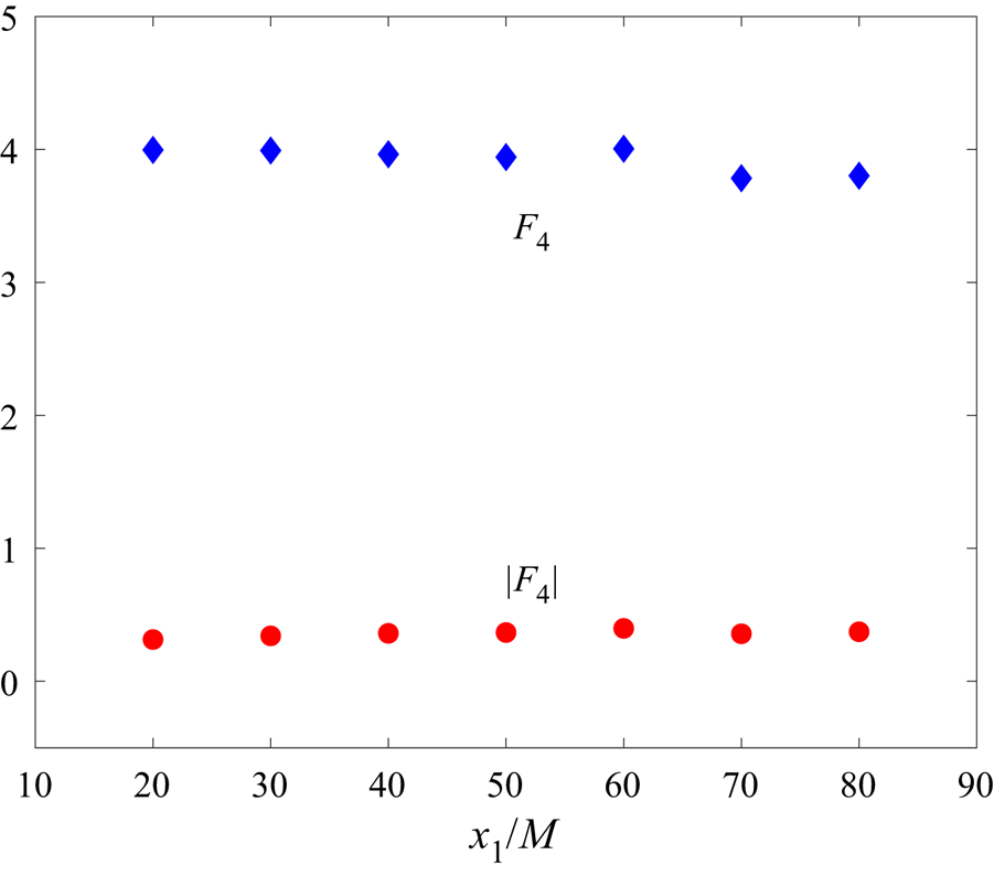
Note that  $F_{n + 1}\approx const.$ along the streamwise direction
 $x_1$ has been used in shearless grid turbulence; this is supported by the data in figure 4. Consequently, the large-scale term in (2.12), viz.
 ${{{C_{n + 2}}}}/{{Re_\lambda }}$ term, is obtained.
Downstream evolution of  $|F_3|$ (
 $\bigcirc$, red) and
 $F_4$ (
 $\diamond$, blue) in shearless grid turbulence at
 $Re_M\approx 10^4$ (unpublished data of Zhou & Antonia Reference Zhou and Antonia2000a).

Appendix D. Derivations of (3.4) to (3.8)
We first derive (3.8) for shearless grid turbulence. After normalizing by  $\overline {{{( {\partial {u_1}/\partial {x_1}} )}^2}}$ and then substituting expressions (A5) and (C2) into the large-scale term in (3.4), the latter becomes
 \begin{align} & {{ - \frac{1}{{n +
1}}{U_1}\frac{\partial }{{\partial {x_1}}}
\overline{{{\left( {\frac{{\partial {u_1}}}{{\partial
{x_2}}}} \right)}^{n + 1}}} }\Biggl/ {{{\overline{{{\left(
{\frac{{\partial {u_1}}}{{\partial {x_1}}}} \right)}^2}}
}^{(n + 2)/2}}}} \nonumber\\ &\quad = {{ - \frac{1}{{n +
1}}{U_1}\frac{\partial }{{\partial {x_1}}} \left( {{F_{y,n
+ 1}}{{\overline{{{\left( {\frac{{\partial
{u_1}}}{{\partial {x_2}}}} \right)}^2}} }^{(n + 1)/2}}}
\right)}\Biggl/ {{{\overline{{{\left( {\frac{{\partial
{u_1}}}{{\partial {x_1}}}} \right)}^2}} }^{(n + 2)/2}}}}
\nonumber\\ &\quad = {{ - \frac{1}{{n +
1}}{U_1}\frac{\partial }{{\partial {x_1}}} \left( {{F_{y,n
+ 1}}R_s^{{ - (n + 1)/2}}{{\overline{{{\left(
{\frac{{\partial {u_1}}}{{\partial {x_1}}}} \right)}^2}}
}^{(n + 1)/2}}} \right)}\Biggl/ {{{\overline{{{\left(
{\frac{{\partial {u_1}}}{{\partial {x_1}}}} \right)}^2}}
}^{(n + 2)/2}}}} \nonumber\\ &\quad = {{ -
\frac{1}{{n + 1}}{U_1}{F_{y,n + 1}}R_s^{{ - (n + 1)/2}}
\frac{\partial }{{\partial {x_1}}}\left(
{{{\overline{{{\left( {\frac{{\partial {u_1}}}{{\partial
{x_1}}}} \right)}^2}} }^{(n + 1)/2}}} \right)}\Biggl/
{{{\overline{{{\left( {\frac{{\partial {u_1}}}{{\partial
{x_1}}}} \right)}^2}} }^{(n + 2)/2}}}} \nonumber\\ &\quad =
\frac{{{F_{y,n + 1}}R_s^{{ - (n + 1)/2}}\dfrac{{5(1 -
m)}}{{ - m}}}}{{R{e_\lambda }}} = \frac{{{C_{y,n +
2}}}}{{Re_\lambda }}. \end{align}
Here,  $F_{y,n + 1}\approx const.$ and
 $R_s \approx const.$ along the streamwise direction
 $x_1$ have been used in shearless grid turbulence. Consequently, the large-scale term in (3.8), viz.
 ${{{C_{y,n + 2}}}}/{{Re_\lambda }}$ term, is obtained.
We now derive (3.8) in sheared grid turbulence. Substituting expressions (3.17), (B4) and (B5) into (3.16) leads to
 \begin{equation} Re_{\lambda_{q}} = \sqrt {\frac{{10{A_q}{Re_M}}}{{3(A + 1)( - {m_1})}}} {\left( {\frac{{{x_1} - {x_0}}}{M}} \right)^{{m_1}/2 + 1/2}}. \end{equation}
Finally, after substituting expressions (B6a,b), (B5) and (D2) into the large-scale term in (3.4), the latter becomes
 \begin{align} & {{ - \frac{1}{{n +
1}}{U_1}\frac{\partial }{{\partial {x_1}}}
\overline{{{\left( {\frac{{\partial {u_1}}}{{\partial
{x_2}}}} \right)}^{n + 1}}} }\Biggl/ {{{\overline{{{\left(
{\frac{{\partial {u_1}}}{{\partial {x_1}}}} \right)}^2}}
}^{(n + 2)/2}}}} \nonumber\\ &\quad = {{ - \frac{1}{{n +
1}}{U_1}{F_{y,n + 1}}R_s^{{ - (n + 1)/2}} \frac{\partial
}{{\partial {x_1}}}\left( {{{\overline{{{\left(
{\frac{{\partial {u_1}}}{{\partial {x_1}}}} \right)}^2}}
}^{(n + 1)/2}}} \right)} \Biggl/ {{{\overline{{{\left(
{\frac{{\partial {u_1}}}{{\partial {x_1}}}} \right)}^2}}
}^{(n + 2)/2}}}} \nonumber\\ &\quad = \frac{{U_1}{F_{y,n +
1}}R_s^{{ - (n + 1)/2}}}{{n + 1}} \frac{{\dfrac{{(1 -
{m_1})(n + 1)}}{{2M}}{{\left( {\dfrac{{(A + 1)( -
{m_1}){A_q}U_1^3}}{{30\nu M{R_{iso}}}}} \right)}^{(n +
1)/2}}{{\left( {\dfrac{{{x_1} - {x_0}}}{M}}
\right)}^{({m_1} - 1)(n + 1)/2 - 1}}}}{{{{\left(
{\dfrac{{(A + 1)( - {m_1}){A_q}U_1^3}}{{30\nu M{R_{iso}}}}}
\right)}^{(n + 2)/2}}{{\left( {\dfrac{{{x_1} - {x_0}}}{M}}
\right)}^{({m_1} - 1)(n + 2)/2}}}} \nonumber\\ &\quad =
\frac{{{F_{y,n + 1}}R_s^{{ - (n + 1)/2}}(1 - {m_1})5\sqrt
{{R_{iso}}} }}{{( - {m_1})(A + 1){Re_{{\lambda _q}}}}} =
\frac{{{C_{y0,n + 2}}\sqrt {{R_{iso}}} }}{{(A +
1){Re_{{\lambda _q}}}}}. \end{align}
Here,  $F_{y,n + 1}\approx const.$ and
 $R_s \approx const.$ along the streamwise direction
 $x_1$ have been used in sheared grid turbulence. It is obvious that the form of the large-scale term in (3.4) is similar for sheared and shearless grid turbulence.