Implications
Housing costs are typically the second-largest cost of pig production after feed cost. Also, the amount of housing area as measured by floor space is a numerical measure used in welfare guidelines for pig production. Thus, this analysis summarized available scientific literature to provide more accurate prediction equations for growth performance across a wider range of inference than previously available. Also, this is the first analysis to quantify the small but meaningful effect of floor space on feed efficiency.
Introduction
Determining ideal floor space for growing pigs is regarded by many as an enigmatic topic. On one hand, reducing floor space decreases gain and feed intake (Gelhbach et al., Reference Gelhbach, Becker, Cox, Harmon and Jensen1966; Gonyou and Stricklin, Reference Gonyou, Brumm, Bush, Deen, Edwards, Fangman, McGlone, Meunier-Salaun, Morrison, Spoolder, Sundberg and Johnson1998), but on the other, it can increase production per unit of housing space (Powell et al., Reference Petherick and Baxter1993). Because of the welfare and economic implications of floor space allowance, accurately predicting its impact on growth could help establish value per unit of floor space to optimize growth rate while still efficiently utilizing space. Kornegay and Notter (Reference Kornegay and Notter1984) calculated the first empirical prediction equations for growing and finishing pigs; however, their database only contained studies with pigs up to 93 kg. Powell et al. (Reference Petherick and Baxter1993) subsequently developed prediction equations for pigs up to 114 kg. However, both sets of equations are outdated for current market weights. Gonyou et al. (Reference Gonyou and Stricklin2006) used transformed values in a broken line allometric model to predict the space requirement of pigs for average daily gain (ADG) and average daily feed intake (ADFI). To date, these equations are viewed as the most applicable prediction equations due to their transformation of the data into percentage changes in ADG and ADFI as the unit of analysis. While this analysis accounts for study-to-study variation, the transformation may result in non-normally distributed error terms. Also, the inclusion criteria required at least one treatment above the k coefficient of 0.030 and at least one treatment below 0.030, limited inclusion of some studies. Therefore, the objective of this study was to utilize data from the existing literature to establish predictive equations for ADG, ADFI and gain : feed ratio (G : F) of finishing pigs dependent on floor space.
Material and methods
A literature review was conducted to compile studies that examined the effects of floor space allowance on ADG, ADFI and G : F of finishing pigs. The literature review and database development used similar techniques as described previously for predicting the effects of net energy on ADG and G : F by Nitikanchana et al. (Reference Nitikanchana, Dritz, Tokach, DeRouchey, Goodband and White2015) and the effects of dietary composition on pork fat iodine value by Paulk et al. (Reference Paulk, Bergstrom, Tokach, Dritz, Burnett, Stephenson, Vaughn, DeRouchey, Goodband, Nelssen and Gonzalez2015). Briefly, the literature search was conducted via the Kansas State University Libraries, utilizing the CABI search engine, and using the keywords ‘space requirement’ or ‘floor space allowance’ with ‘finishing pig’ or ‘growing pig.’ Data were derived from both refereed and non-refereed publications including theses, electronic publications and university publications. Each publication was screened to ensure that there were at least two-floor space treatments. The initial screen yielded 37 publications. In addition, to be included in the final database, experiments had to meet the following criteria: first, pigs used in the experiments had to have ad libitum access to feed and water; second the materials and methods had to provide management information including treatment means, feeder space, water space, group size and floor type; and third the studies had to have a reported standard error (SE) or SD for treatment means. Papers were eliminated from the analysis for not allowing ad libitum access to feed and water (one paper), lack of treatment means (one paper), failure to report SE or SD to calculate an SE (three papers), or not including information associated with feeder space, water space or group size (two papers). Also, only studies with a minimum initial BW of 18 kg were used due to lack of information at lighter BWs. Papers that did not calculate study length or final BW were included in the database and the missing information was calculated by using ADG, initial BW and either study length or final BW. For papers that reported feed efficiency as feed : gain ratio (F : G), an inverse proportion was calculated using ADG and ADFI values. This value was then used to convert the related SEs associated with the F : G information. Briefly, the estimates were converted to a SD (SD=SE×√n), then a CV (SD/mean) was calculated, the CV was then used to calculate a SD (CV×G : F) for the G : F proportion, this value was then transformed back to a SE (SD/√n=SE). The coefficient k (k=floor space m2/BW0.67) was calculated for all experimental units based on the final BW of the growth period and the associated floor space allowance. Growth performance over the entire study length for each experimental unit was used in the database, except if floor space allowance was adjusted across phases. In these instances, where individual phase performance was reported the growth periods associated with the floor space allowance provided were used as individual observations.
Flooring type (partially slatted or fully slatted concrete) used in each study was also accounted for in the prediction models. Water space was calculated as the number of pigs per waterer within a pen. In studies where wet/dry feeders were used, each feeder space was also considered a waterer. Feeder space was calculated as the number of pigs per feeder hole. Gender was also categorized as a potential predictor variable. There were four papers that presented floor space treatments for barrows and four papers that reported floor space treatments for gilts. All other papers either contained mixed gender pens (barrows and gilts) or reported main effect means without separating gender×floor space treatment interactions. Due to the low number of observations that included data by gender the effects within gender or interactions with gender were not modeled. However, these observations were maintained in the final model. The final database for studies examining the influence of floor space allowance resulted in 30 papers with 112 observations for ADG, and 28 papers with 107 observations for ADFI. The final database resulted in publication dates from 1983 to 2014 (Supplementary Material Table S1).
Statistical analyses for model development
Mixed model methodology described by St-Pierre (Reference St-Pierre2001) to collate quantitative values across multiple studies was used. These methods were used to develop regression equations separately predicting ADG and ADFI dependent on floor space. The floor space treatment applied within each experiment was the observational and experimental unit and thus served as the residual error term. The method of maximum likelihood was used in the model selection to evaluate the significance of fixed effect terms. Once the ADG and ADFI models were determined the predicted values for each observation were output and the G : F model was developed. Random effects included in the model were decade, paper within decade, and experiment within paper×decade interactions. Decade was included as a random effect to account for random error associated with the increases in growth rate over time (Knap, Reference Knap2009). Paper within decade was used to account for random error observed between papers within the same decade. Experiment within paper×decade interaction was used to account for random error observed from experiment to experiment within each paper×decade interaction. The error between decades, papers within decades and experiments within paper×decade interactions were partitioned using the repeated statement. Covariance parameter estimates were different, emphasizing the use of these random effects in the model selection process across decade and paper. Including these random effect terms lead to significant decreases in in the Bayesian information criterion (BIC). Also, to account for variance and replication differences across studies the inverse of the SE was used as a weighting factor in the model using procedures presented by St-Pierre (Reference St-Pierre2001). Weighting the observation using the SE resulted in a reduced residual covariance estimate, supporting their use for the model fitting process.
Candidate terms for the modeled equations were selected by evaluating the single variable predictors. The initial model was fit using the single predictor of k in the model with the random effects. As expected k had the lowest BIC for all the single variable predictors. The threshold level of significance for single variable terms inclusion was P<0.10. The single variable term with the lowest BIC was initially evaluated and terms were then added to the models in a step-wise manual forward selection process based on improvement in the BIC. A model comparison with a reduction in BIC of more than 2 was considered an improvement (Kass and Raftery, Reference Kass and Raftery1995). Throughout the selection process, studentized residuals plots were observed to determine if quadratic or interaction terms were needed. Per the hierarchy principle, even if the lower order terms were not significant, they were retained in the model (Peixoto, Reference Powell, Brumm and Massey1987).
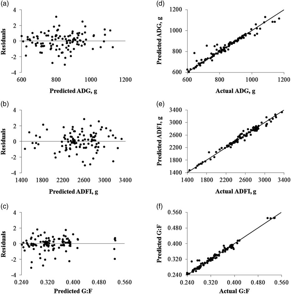
The method of residual maximum likelihood was then used to obtain the estimate of the parameters for the candidate models. These models were also examined by evaluating a histogram of the residuals for evidence of normality and plotting residuals against predicted values of Y (ADG, ADFI and G : F of finishing pigs within each set of databases; St-Pierre, Reference St-Pierre2001). Residual plots were also used to investigate outliers. Any residual >3 standard deviations from the mean were deemed outliers for review. Outliers were then reviewed to determine if they were biologically significant. As a result, three observations for finishing ADG, ADFI and G : F in both databases were removed from the analysis. Finally, due to the inclusion of peer reviewed (23) and non-peer reviewed (seven) publications (thesis and technical memos) the studentized residuals from the final model were categorized as peer or non-peer reviewed and plotted for visual evidence of patterns suggesting heterogeneity or bias across the two categories. The means from the two categories of the residuals were then compared using a t-test and there was no evidence suggesting difference. Thus, all non-peer reviewed publications were maintained in the final model. The PROC MIXED procedure of SAS (SAS Institute Inc., Cary, NC, USA) was used for all statistical modeling.
Statistical analyses for model performance
Regression analysis of the predicted values dependent on the observed values was performed for model performance using methods suggested by Tedeschi (Reference Tedeschi2006). The coefficient of determination (r 2) was calculated to evaluate the precision of the model-predicted values to the observed values by describing the proportion of variance in the observed values described by the predicted values. Mean bias was used to assess model accuracy and was computed by subtracting the mean of the observed values minus the mean of the predicted values. The mean bias was expressed in g for ADG and ADFI. A positive mean bias would indicate an underestimation and a negative value indicates an overestimation by the prediction equation. Also, observed values were plotted against predicted values to evaluate the line of equality and determine if there was bias in the estimations (Altman and Bland, Reference Altman and Bland1983). This bias was further quantitatively evaluated by calculating a bias correction factor (C b ). This method measures the accuracy of the model-predicted values to the observed values by examining how far the regression line deviates from the slope of unity. A range of 0 to 1 can be observed for the bias correction factor with a value of 1 indicating there is no deviation of the regression line from the line of unity.
Next a reproducibility index was developed and termed the concordance correlation coefficient (CCC) using methods suggested by Tedeschi (Reference Tedeschi2006). This coefficient was used to simultaneously assess both precision and accuracy of the model by utilizing the correlation coefficient (r), mean bias, and the bias correction factor in its calculation. A value of 1 or −1 implies perfect concordance or disconcordance. While a value closer to zero denotes the absence of agreement between the variables. Root mean square error of prediction (RMSEP) was used to measure the predictive accuracy of the model. This was calculated as the cumulative variation between the observed values and model-predicted values. The model efficiency statistic (MEF) which is interpreted as the proportion of variation explained by the line Y=ƒ(X 1 , … ,X p ) was calculated. A value of one would indicate a perfect fit and if the MEF value is less than zero, the model-predicted values are more variable than the observed values. Finally, a coefficient of model determination was established. The coefficient is defined as a ratio of the total variance of observed data to the square of the difference between the model-predicted mean and mean of the observed data. A ratio <1 suggests an overestimation of the total variance observed in the model-predicted values, and a value >1 suggests an underestimation of the total variance by the predicted values.
Results
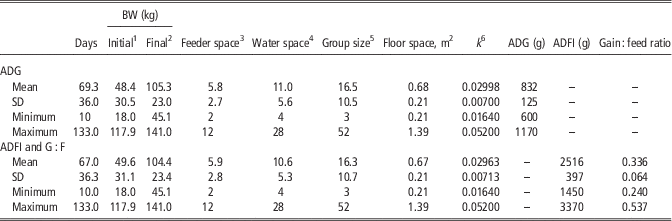
Descriptive statistics are presented in Table 1. These values depict the floor space, feeder space, water space, floor type and study length from finishing swine experiments throughout the literature. They also portray the range of growth performance and BW throughout experiments used to develop the models. Residuals v. predicted values and actual values v. predicted values indicate that model assumptions were valid (Figure 1).
Studentized residual plots when modeling the effect of floor space values on pig growth performance (a) average daily gain (ADG), (b) average daily feed intake (ADFI), and (c) gain : feed ratio (G : F), and plots of actual values v. predicted values relative to the line of equality for (d) ADG, (e) ADFI, and (f) G : F. The plots for ADG are based on 112 observations from 30 papers and 107 observations from 28 papers for ADFI and G : F.

Descriptive statistics for data included in prediction models for the effects of floor space on finishing pig growth performance

ADG=average daily gain; ADFI=average daily feed intake
1 Refers to the BW of pigs at the beginning of the experiment.
2 Refers to the BW of pigs at the end of the experiment.
3 Number of pigs per feeder hole.
4 Number of pigs per waterer.
5 Number of pigs per pen.
6 Coefficient k is the constant in the equation k=floor space (m2)/BW0.667.
Average daily gain
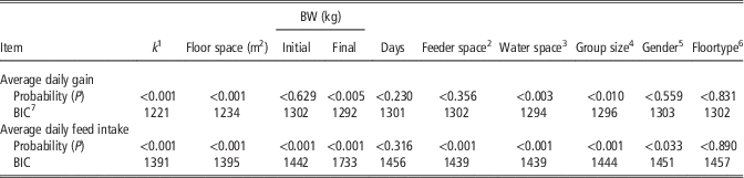
For ADG, using k as a single predictor variable resulted in the lowest BIC value (Table 2). Therefore, k was the first predictor variable selected for the models. Also, an increasing k was a significant predictor of increased ADG (P<0.01). However, when examining the studentized residuals clear quadratic trends were evident suggesting that increasing k increased ADG but at a diminishing rate; thus, k 2 was added and was a significant predictor (P<0.001) of ADG as well as lowering the BIC value compared with the model containing only the linear term of k. Next, initial BW was included but was not a significant predictor of ADG (P=0.233). Although, after examining the residuals of the model with BW it appeared that for observations with heavier initial BW, as k increased the predicted values continued to underestimate ADG suggesting the need for a k×initial BW interactive term. Its inclusion increased ADG as k or as initial BW were increased and was useful (P<0.006) as a predictor of ADG and resulted in models with the lowest BIC values. Although not significant, based on the hierarchy principle the single variable term for initial BW was retained in the model. Including final BW resulted in a significant coefficient for BW (P=0.013) as well as lowering the BIC value. This resulted in a model with the lowest BIC value (1183; Table 3).
Single variable models used to predict average daily gain and average daily feed intake for finishing pigs

1 Coefficient k is the constant in the equation k=floor space (m2)/BW0.67.
2 Represents the number of pigs per feeder hole.
3 Represents the number of pigs per waterer.
4 Group size represents the number of pigs per pen.
5 Gender for each database consisted of barrow, gilt and mixed (barrow and gilt) information.
6 Floor types observed for finishing databases were partially and fully slatted concrete flooring.
7 Bayesian information criterion (BIC) values were used to compare the precision of the model.
Regression equations generated from existing data for average daily gain (ADG), average daily feed intake (ADFI) and G : F for finishing pigs

Examining the model fits (Table 4), it appeared the model-predicted values had a mean bias of −1.6 g/day. The coefficients of determination (r 2=0.949) suggested that almost 95% of the variation observed in the actual values were explained by the model-predicted values. This agrees with the MEF statistics (MEF=0.948) generated. In addition, the bias correction factors (C b =0.999) were high, suggesting the regression line was closely related to the line of unity. Next, the reproducibility indexes was also high (CCC=0.989), indicating strong agreement between the observed and model-predicted values. The coefficients of model determination were >1 (CD=1.13) suggesting that the model-predicted value underestimated the total variance in the observed values by ~13%. The RMSEP (28.7 g/day) indicates >93% of the error associated with the model was random error.
Evaluation of model fit to databases for prediction equations for finishing pig growth

1 Coefficient of determination (Neter et al., Reference Neter, Kutner, Nachtsheim and Wasserman1996). Values measure the fit of the residual variance and do not infer information from random effects in the model; therefore, they are higher than a simple fixed effect model.
2 Mean bias was computed by subtracting the mean of observed values minus the mean of the predicted values (Cochran and Cox, Reference Cochran and Cox1957). A negative value insinuates an overestimation.
3 Bias correction factor (C b ) is a component of the CCC statistic that indicates how far the regression line deviates from the slope of unity (45°; Lin, 1989).
4 Concordance correlation coefficient (CCC), also known as reproducibility index, assesses both the precision and accuracy of the model (Lin, Reference Lin1989).
5 Root mean square error of prediction (RMSEP) is used to measure the predictive accuracy of the model (Mitchell, Reference Mitchell1997).
6 Modeling efficiency statistic (MEF) is used as an indicator of goodness of fit (Mayer and Butler, Reference Mayer and Butler1993). A MEF value closer to 1 suggests better fit and a value less than zero indicates that the model-predicted values are worse than the observed mean.
7 The coefficient of model determination (CD) explains the proportion of the total variance of the observed values explained by the predicted data. The closer the CD value to 1 the better, with ratios over 1 insinuating model under prediction of total variance, and a ratio <1 suggesting an overestimation of the total variance by the model.
Average daily feed Intake
For ADFI model, k was a significant single predictor of feed intake and increasing k is associated with an increase in ADFI (P<0.01). Also, using k as a single predictor variable resulted in the lowest BIC values when compared to the BIC values in the other single variable models (1175). Therefore, k was the first predictor variable selected for candidate models. When examining the studentized residuals resulting from the models clear quadratic trends were evident for k suggesting that increasing k increased ADFI but at a diminishing rate. Thus, k 2 was added to the models as a significant predictor (P<0.003) which lowered the BIC values. Initial BW was also a predictor (P<0.056) of ADFI, because increasing initial BW decreased ADFI, which reduced the BIC values (1123 and 1332 for database 1 and 2, respectively). Finally, similar to ADG, the inclusion of a k×initial BW interaction (P<0.001) reduced the BIC to their lowest values, and with its inclusion in the models, increasing k or initial BW resulted in an increased ADFI. Final BW was then included as a significant (P<0.01) predictor of ADFI, because ADFI increased within increasing final BW. The resulting models had the lowest BIC value with the fewest terms of any candidate models evaluated
When examining the model fit, it appeared the model-predicted values were close to actual values, with mean bias of 0.06 g/day. The coefficient of determination (0.978) suggesting that ~98% of the variation observed in the actual values were explained by the model-predicted values. This agrees with the MEF statistics (MEF=0.978) that ~98% of the variation associated with the responses were explained by the fitted model-predicted lines. In addition, the bias correction factor (C b =0.999) was high, suggesting the regression lines were closely related to the lines of unity, and the reproducibility index was also high (CCC=0.990), suggesting strong agreement between the observed and model-predicted values. The coefficients of model determination were >1 (CD=1.04) suggesting that the model-predicted values underestimated the total variance in the observed values by ~4%. The RMSEP 59.2 g/day and indicated that >98% of the error of the models was random error.
Gain : feed ratio
For finishing G : F models, using the predicted ADG/predicted ADFI values for both databases resulted significant predictions of G : F (P<0.001). The 95% confidence interval on the coefficient for the term was 0.995 to 1.003. The coefficient of 1.00 was observed in the 95% confidence interval range, which indicates predicted ADG/predicted ADFI had a coefficient where there was a lack of evidence that it was different than 1, which supports their use as a predictor of G : F. When evaluating the fit of the G : F models to their databases, the mean bias was −0.0007. The coefficient of determination (r 2=0.978) suggested that ~98% of the variation observed in the actual values were explained by the model-predicted values. This agrees with the MEF statistics (MEF=0.977) that almost 99% of the variation associated with the responses are explained by the fitted model-predicted lines. In addition, the bias correction factors (C b =0.999) were high suggesting the regression line was closely related to the line of unity, and the reproducibility index was also high (CCC=0.988), suggesting strong agreement between the observed and model-predicted values. The coefficients of model determination were slightly >1 (CD 1.04). The RMSEP was 0.010 which indicated that >99% of variation in the model error term was random error.
Discussion
Historically, floor space allowance has been expressed in the literature as the amount of space per pig. The difficulty with this approach is that as pigs grow, their requirement for space grows as well. To alleviate this challenge, the use of an allometric tool to convert the three-dimensional term of weight to a two-dimensional measure of area was used as the expression of floor space: A=k×BW0.67. Where A represents floor space allowance in m2, k represents a constant coefficient, and BW0.67 in kg represents the geometric conversion of weight to area. This assumes that as BW increases the animal’s surface area requirement increases proportionately. The increased proportion of variance accounted for when k is used as single initial predictor compared with floor space alone suggests this assumption is valid. The first to propose this method was Petherick and Baxter (Reference Peixoto1981) with others adopting it to provide a consistent area of space as the animal grows. In fact, many space recommendations are based on k (AAFC, 1993; European Community, 2001).
Shull (Reference Shull2010) discussed one discrepancy with the use of the allometric measurement k. Does the pig’s requirement for space grow proportionately to BW0.67? This assumption is based off the geometric principle that increasing the volume of a cube results in a proportional increase in the surface area of each side. There is little research truly examining whether this function captures the true changes in the pig’s space requirement as it increases in BW. Interestingly, the models were further improved with the inclusion of initial and final BW terms. Thus, the multivariable models herein would indicate that the change in floor space requirement indicates an improvement in the description of floor space requirement. This is an indication that the two-dimensional space requirement for pigs is most likely not perfectly related to their three dimensional volume and consistent with the concept that a pig is not a perfect cube. Therefore, we believe the improvement in fit of the models when describing floor space as a function of BW and k may describe the biological response more accurately than using k alone.
Furthermore, the improvement in fit of current models with additional predictors in addition to k suggest use of the single predictor allometric coefficient k fails to account for BW interactions with floor space allowance. And thus, the multi-term models herein use initial and final BW, along with a k×initial BW interaction, as predictor terms for growth. This means there is different critical k thresholds (requirements) based on the BW range of finishing pigs that are being examined. Kornegay and Notter (Reference Kornegay and Notter1984) were the first to use linear and curvilinear analysis to describe the impact of floor space allowance on growth criteria. Their empirical equations, developed for growing and finishing pigs, were single variable prediction models with floor space as the predictor variable in which increasing floor space improved performance parameters at a decreasing (quadratic) rate. The drawbacks to their prediction equations were that they did not account for BW influences on response criteria, and with the statistical capabilities of the time, their models were simple fixed effect models which did not account for known random error terms that could impact responses. Another limitation from their data was the heaviest observed BW was 93 kg which is much lower than current market weights.
The most recently developed summary of the floor space literature included linear broken-line space requirement curves based on the allometric coefficient k (Gonyou et al., Reference Gonyou and Stricklin2006). To account for study-to-study variation the authors transformed the data as a percentage of the maximum response. This allows for an equation that is easily interpretable across a wide variety of different production environments. This has resulted in their wide acceptance as a standard for estimating the influence of floor space allowance on ADG and ADFI. Initially, we tried to model the data using similar methods. However, due to the constraint of classifying all responses on a percentage basis we observed significant patterns in the studentized residuals that failed to support the assumption of normal distribution. However, using general linear mixed models with predictor variables to directly predict ADG and ADFI from an analysis of the current literature database the model assumptions for normality were met. This suggests our modeling procedure is significantly more robust than that used by Gonyou et al. (Reference Gonyou and Stricklin2006) Also, the current analysis used weighted observations to account for differences in experimental design and replication across papers and experiments to help improve the precision of estimates and lower the residual error of the prediction models. The weighting by the inverse of the SE allowed studies with less variability of the estimate to be more heavily weighted in the evidence. Also, this allowed treatment means with the same standard deviation but higher mounts of replication to have increased weight in the analysis
When Gonyou et al. (Reference Gonyou and Stricklin2006) included studies into their database, they only accepted studies in which at least one floor space treatment was above the k coefficient of 0.030 and at least one observation was below that same threshold. In total, the authors had 11 published papers that were used to estimate the space requirement of finishing pigs. However, the database of peer-reviewed published literature available prior to publication of the prediction equations included an additional nine studies. It appears these studies were not included due to the stringent k threshold for study inclusion. The lack of inclusion of these studies may have biased the threshold response closer to k=0.030. The models developed herein used a total of 92 and 112 observations in their respective databases which is more than three times the size of the database used by Gonyou et al. (Reference Gonyou and Stricklin2006) to predict ADG and ADFI.
Another important factor is that values of k were calculated for all observations without restrictions on the inclusions of values. In addition, since the publication of Gonyou et al. (Reference Gonyou and Stricklin2006) more research has been conducted with finishing pigs at heavier weights, providing more information on how BW alters the impact floor space allowance on growth. These two factors led to a curvilinear model where a true plateau or end to space restriction was not observed across the ranges of k and initial and final BW evaluated. Fundamentally, we know that eventually a plateau does occur but we were unable to delineate a breakpoint based on the data ranges for the predictor variables. Also, this indicates that the impact of space restriction on growth changes as either initial or final BW changes. This indicates that the breakpoint differs and the slope differs based on weight range of the pig evaluated. In contrast, the equation provided by Gonyou et al. (Reference Gonyou and Stricklin2006) assumed a constant slope and breakpoint. Subsequent studies have indicated that growth rate is impacted at a lighter BW than suggested by the Gonyou et al. (Reference Gonyou and Stricklin2006) equation (Thomas et al., Reference Thomas, Goodband, Tokach, DeRouchey, Woodworth and Dritz2015; Flohr et al., Reference Flohr, Tokach, DeRouchey, Woodworth, Goodband and Dritz2016). Also, the curvilinear approach and initial BW interaction with k is useful for predicting the impact of growth rate when pigs have been marketed from the pen. Removal of the pig essentially changes the space available. Indeed, in the subsequent validation work by Flohr et al. Reference Flohr, Tokach, DeRouchey, Woodworth, Goodband and Dritz2016 we have confirmed a lack of a breakpoint when marketing pigs at heavy weights (135 to 145 kg BW) under practical commercial ranges of space allowance.
Next, the impact of floor space allowance on feed efficiency is a perplexing topic. There are several proposed modes of actions for the worsened feed efficiency caused by reduced floor space allowance. Chapple (Reference Chapple1993) proposed that rearing pigs in groups reduces the capacity of the pig to deposit protein resulting in reduced feed intake and worsened feed utilization. Zhang et al. (2013) reported a linear reduction in N digestibility and blood urea nitrogen for 25 kg pigs stocked at 0.64, 0.48 and 0.38 m2 for 36 days. Shull (Reference Shull2010) has implicated the potential for increased feed wastage and energy expenditures due to increased trips to the feeder caused by more interruptions during feeding. It may be that reducing floor space allowance leads to multiple behavioral changes that could impact growth and metabolism. Most researchers have not necessarily focused on the impact of floor space allowance on feed efficiency because the response seems to be a lower magnitude and more variable than that of ADG and ADFI. Previous equations to estimate the impact of floor space allowance on feed efficiency were proposed by Harper and Kornegay (Reference Harper and Kornegay1983) and by Powell et al. (Reference Petherick and Baxter1993); however, Gonyou et al. (Reference Gonyou and Stricklin2006) concluded that feed efficiency was not impacted by floor space allowance. Most papers conclude that there is no evidence for statistical differences in G : F with varying floor space allowance; however, most studies see increased final BW as floor space allowance is increased. So, it begs to question; is the influence of floor space allowance on feed efficiency potentially veiled by changes in final BW between treatments? While a few of the papers utilized in the database reported statistical evidence for an impact of floor space on feed efficiency, a majority of studies observed numerically improved G : F. Although the response may not be to the same magnitude as ADG and ADFI, examining the available literature suggests that feed efficiency is impacted by floor space allowance. This illustrates the value of combining studies in a meta-analysis framework to describe small but significant relationships.
Interestingly, the prediction equations herein did not find any other environmental factors (group size, feeder space or water space) as significant predictors of growth in the multivariable models. However, that does not mean that potential interactions with these factors and floor space allowance do not exist. The magnitude was not large enough to be included in our final models. In fact, the amount of research examining the effects of water space (pigs per waterer) on growth is surprisingly limited. The Midwest Plan Service (1991) recommends one water space per 10 weaned pigs and for 15 growing pigs. However, this recommendation makes no mention of different waterer forms that are available. Also, within this analysis, feeder space was a general term used to describe the number of pigs per feeder hole. Ideally, a more descriptive term that includes a characterization of the feeding space quality would have been preferred; however, the number of pigs per feeder hole was the only consistently reported value across papers included in the databases. Additional information regarding trough space per pig, along with feeder design would have helped describe potential feeder effects on growth performance.
In summary, floor space allowance is an important environmental factor that influences finishing pig growth. The regression equations herein provide good alternative estimates of ADG, ADFI and G : F based on BW and k in order to predict finishing pig growth performance when provided different floor space allowances. Compared to previous equations, the models herein were developed using general linear mixed models from a larger database and with additional information at heavier BWs than previously summarized.
Supplementary material
To view supplementary material for this article, please visit https://doi.org/10.1017/10.1017/S1751731117002440