1 Introduction
Turbulence drastically decreases mixing times among reactants in any flow regime, and scramjet engines in particular would benefit from gaining a certain control authority on its dynamics and spatial distribution within the combustor, where the flow is largely supersonic. Because of the high speeds, the residence time of the flow within the combustor of a hypersonic air breathing engine is of the order of 1 ms and, therefore, the combustion process is mixing limited. A systematic study of turbulence dynamics in these complex flows will provide the tools to address and solve the aforementioned issue.
Due to their decreased sensitivity to compressibility effects when compared to the spanwise structures in planar shear layers, streamwise vortical structures have always attracted the interest of researchers in the field of supersonic mixing. Additionally, the increased turbulence levels associated with their straining action in the flow and the possibility to re-orient and re-distribute the vorticity due to its vectorial nature by means of specific vortex interactions, make these vortices the preferential candidates for mixing augmentation in scramjet injection strategies.
Although molecular mixing is accomplished at the smallest scales and accelerated by the action of turbulence, two fundamental contributions to the process come directly from the mean flow: the entrainment of irrotational fluid into the vortices and the strain rates introduced by the large-scale, vortical motion at the interface between the reactants (Marble Reference Marble1985; Waitz et al. Reference Waitz, Qiu, Manning, Fung, Elliot, Kerwin, Krasnodebski, O’Sullivan, Tew and Greitzer1997). This can also be seen in the one-dimensional equation for the species concentration transport:
 $$\begin{eqnarray}\frac{\unicode[STIX]{x2202}K}{\unicode[STIX]{x2202}t}=\unicode[STIX]{x1D716}n\frac{\unicode[STIX]{x2202}K}{\unicode[STIX]{x2202}n}+D_{t}\frac{\unicode[STIX]{x2202}^{2}K}{\unicode[STIX]{x2202}n^{2}},\end{eqnarray}$$
where
 $n$
is the axis normal to the interface,
 $K$
is the concentration,
 $\unicode[STIX]{x1D716}$
is the normal strain rate and
 $D_{t}$
is the binary, turbulent diffusion coefficient.
In addition, strain rates are also responsible for increasing the turbulence levels as they allow relatively large amounts of energy to be extracted from the mean flow and converted into turbulent motion, as can be seen in the production term of the turbulent kinetic energy (
 $TKE$
) transport equation:
 $$\begin{eqnarray}P_{TKE}=-\langle u_{i}^{\prime }u_{j}^{\prime }\rangle \unicode[STIX]{x1D61A}_{ij},\end{eqnarray}$$
where
 $\unicode[STIX]{x1D61A}_{ij}$
is the mean strain rate tensor and
 $u_{i}^{\prime }$
,
 $u_{j}^{\prime }$
are the velocity fluctuations.
The proper selection of the aforementioned vortex interactions and the consequent generation of mean strain rates in specific areas of the flow could potentially allow both the manipulation of entrainment and the mixing enhancement in supersonic flows.
Effects of streamwise vortices on mixing and mixing efficiency have been experimentally studied in the past. One of the initial works on vortex-enhanced mixing in subsonic flows was conducted by Chigier & Chervinsky (Reference Chigier and Chervinsky1967). In that combined theoretical and experimental investigation, it was demonstrated that entrainment of fluid within a swirling jet increased linearly with the degree of swirl, suggesting increased spreading and better mixing when streamwise vortices are introduced within a turbulent jet. Swithenbank & Chigier (Reference Swithenbank and Chigier1969) attempted a generalization of the concepts proposed in the earlier work from Chigier & Chervinsky (Reference Chigier and Chervinsky1967) to supersonic flows. They presented an extensive review of the principal phenomena related to turbulent mixing and postulated that streamwise vortex systems introduced in jets or wakes developing in supersonic flow would be beneficial in the mixing processes for scramjet combustors. However, very few arguments were presented for the actual supersonic case as the authors pointed out that further work was needed to assess the effectiveness of subsonic or transonic swirling jets in the mixing process with an external high-speed flow. From that point, a common approach of the studies on scramjet fuel injection concepts has been to aim at increasing the streamwise vorticity in the combustor by means of ramps, which have been extensively tested in the past (Donohue & McDaniel Reference Donohue and McDaniel1996; Aso et al. Reference Aso, Yamane, Ando, Umii, Tokunaga and Sakata1997; Schumacher Reference Schumacher2000; Inoue & Aso Reference Inoue and Aso2004; Koike et al. Reference Koike, Suzuki, Kitamura, Hirota, Takita, Masuya and Matsumoto2006; Kondo, Sakaue & Arai Reference Kondo, Sakaue and Arai2008; Kondo et al. Reference Kondo, Hayase, Sakaue and Arai2009; Arai et al. Reference Arai, Sakaue, Hayase, Hiejima, Sunami and Nishioka2011), or transverse jets (Billig & Schetz Reference Billig and Schetz1992). However, the effects of the resulting vortical structures on the turbulence and consequent losses introduced in the flow are still unexplored.
Some works have been dedicated to the understanding of the mean motion of supersonic vortical structures, but relatively limited research has been conducted in the field of turbulence in this class of flows. Particle image velocimetry (PIV) greatly helped to obtain information on the spatial distribution of turbulence across relatively large cross-sections of the flows under consideration, overcoming the inevitable limitations of hot-wire anemometry. PIV is, in fact, currently the state-of-the art for flow velocity measurements, but can still be poisoned by uncertainties if great care is not used in the experimental design and set-up, especially when applied to supersonic flows. Additionally, the convergence of the turbulence statistics requires the collection of a large amount of data, implying the execution of extensive and sometimes not cost-effective wind-tunnel campaigns. Therefore, it can be conjectured that one of the reasons for this lack of turbulence data may be due to both in the difficulty of assessing the degree of reliability of PIV measurements as well as to the necessity for prohibitive experimental campaigns.
Smith & Goyne (Reference Smith and Goyne2011) adopted stereoscopic PIV (S-PIV) to study the flow field resulting from the streamwise counter-rotating vortex pair shed from a ramp mounted in a dual-mode scramjet combustor, both in a reacting and non-reacting environment. The work first presented the detailed description of the S-PIV system and its use in the challenging experimental conditions along with the related uncertainties, then provided the measurements of the mean flow fields and turbulence intensity in the plumes for the reacting and non-reacting cases. The discussion was mostly focused upon the differences of the mean flows for the two cases considered, but only marginally on the turbulence intensities and no attempt was made to find a connection between them and any of the relevant quantities typical of the streamwise structures shed from the ramp (i.e. circulation, size of the vortices).
Beresh et al. (Reference Beresh, Henfling, Erven and Spillers2006) presented high-quality stereoscopic PIV turbulence statistics of a counter-rotating vortex pair (CVP) developing in a transverse jet into a transonic cross-flow. The work directly relates to previous measurements conducted by the same authors in the streamwise direction (Beresh et al.
Reference Beresh, Henfling, Erven and Spillers2005) while providing, additionally, fundamental data at least in one of the downstream cross-planes which, according to Beresh et al. (Reference Beresh, Henfling, Erven and Spillers2006), are rare to find in scholarly work. The manuscript presented measurements in one streamwise cross-section of the flow for increasing fuel-to-free stream momentum flux ratios (i.e.
 $J$
). Among the outcomes of the research (some interesting conclusions were drawn for the mean flow quantities), the trends of the Reynolds stresses and
 $TKE$
were given for one value of
 $J$
to provide useful data for the improvement of turbulence models for this class of flows. Unfortunately, despite the great care put in the experiments as well as the quality of the measurements, the analysis of the fluctuating flow data could not yield more general conclusions on the physics and the dynamics of turbulence within the CVP due to the lack of cross-flow sections inspected.
For all these reasons, turbulence databases in supersonic flow are still rather incomplete. Especially in the context of supersonic streamwise vortices, significant work is missing despite the widespread recognition that these structures increase the strain rates in the flow, directly affecting the production of turbulent kinetic energy. Therefore, vortices of different scales and strengths resulting, for example, from complex interactions, may have a non-negligible effect on the turbulence content of the flow which is worth exploring due to the possible application of these structures to both internal (mixing and combustion) and external aerodynamics (wing-tip vortices).
More complete is the turbulence database in subsonic flows where many semi-empirical turbulence decay relations have been proposed, based mostly on grid-generated turbulence, in an effort to better understand the physics underlying the decay of isotropic and homogeneous turbulence (George & Wang Reference George and Wang2009; Hearst & Lavoie Reference Hearst and Lavoie2014; Isaza, Salazar & Warhaft Reference Isaza, Salazar and Warhaft2014; Sinhuber, Bodenschatz & Bewley Reference Sinhuber, Bodenschatz and Bewley2015). Valente & Vassilicos (Reference Valente and Vassilicos2011) provided a review of existing models for the description of the decay of homogeneous and isotropic turbulence in addition to presenting experimental data on turbulence generated by multiscale grids. Those results showed a faster decay compared to the commonly accepted power-law-based dissipation rates (Taylor Reference Taylor1935; Batchelor Reference Batchelor1959; Pope Reference Pope2000). As part of the review of the models for homogeneous and isotropic turbulence decay, a generally accepted scaling law was also reported, which included the dependence of the
 $TKE$
from the grid Reynolds number
 $Re_{0}$
as well as the streamwise distance
 $x$
relative to a virtual origin
 $x_{0}$
and non-dimensionalized by the length scale of the inlet
 $L_{B}$
(see (1.3)).
 $$\begin{eqnarray}\sqrt{TKE}\frac{\unicode[STIX]{x1D706}}{\unicode[STIX]{x1D708}}\propto Re_{0}^{1/2}\left(\frac{x-x_{0}}{L_{B}}\right)^{m/2-n/4},\end{eqnarray}$$
where
 $\unicode[STIX]{x1D706}$
is the Taylor microscale,
 $\unicode[STIX]{x1D708}$
is the kinematic viscosity and
 $m$
and
 $n$
are exponents which depend on the class of flow considered: plane wakes, axisymmetric wakes, self-propelled plane wakes, self-propelled axisymmetric wakes, mixing layers, plane jets, axisymmetric jets and regular grid turbulence.
Lately, interactions among the vortical structures have been found crucial for targeting specific modifications of the plume’s morphology (Maddalena, Vergine & Crisanti Reference Maddalena, Vergine and Crisanti2014). Thus, the first step towards the optimization of injection strategies based on streamwise vortex mixing for scramjet combustors is the understanding of the modifications introduced by the large-scale motion down to the smaller scales. A vortex interaction-based approach to increase the vorticity content and strain rates in a particular area of the flow is through the merging of co-rotating structures, which can happen in subsonic flow and, under controlled conditions, in a supersonic flow regime as well. Vortex merging has been analysed in incompressible flow in the past (Cerretelli & Williamson Reference Cerretelli and Williamson2003; Meunier, Dizs & Leweke Reference Meunier, Dizs and Leweke2005) and recently documented, with the support of reduced-order simulations, in the supersonic regime. In particular, Maddalena et al. (Reference Maddalena, Vergine and Crisanti2014) demonstrated the ability of a computer code (i.e. VorTx), based on an inviscid supersonic flow model developed by the authors, to predict the complex flow physics behind the merging of co-rotating structures in supersonic cold flow.
VorTx was also used by Vergine & Maddalena (Reference Vergine and Maddalena2015) to design an experimental campaign aimed at analysing of the mean flow fields resulting from vortex merging and non-merging scenarios in a Mach 2.5 cold flow. The reduced-order simulations were presented and the inviscid nature of the evolving streamwise vortices of given strength (i.e. circulation of the order of
 $1~\text{m}^{2}~\text{s}^{-1}$
) was assessed along with their entrainment capability. However, no turbulence data were provided, leaving unanswered the question on any possible differences in turbulence levels between merger and isolated vortices.
It is thus clear that the characterization of the modifications in the fluctuating cross-flows introduced by merging and non-merging streamwise vortices is a key point that must be addressed.
Therefore, in addition to briefly summarizing part of the mean flow results of the two aforementioned vortex interaction scenarios, the first part of this work (presented in § 4) analyses in depth the characteristics and the dynamics of turbulence within the same supersonic vortical structures through the use of S-PIV (see § 2.1). Specifically, the same streamwise vortices have been considered to experimentally investigate a case where the resulting dynamics evolves in a vortex merging scenario (case I) and a case where the merging process is avoided (case II), as prescribed by the outcomes of reduced-order, inviscid simulations conducted with VorTx. The streamwise vortices are generated by means of expansion ramps placed on the surface of a strut injector and develop in its wake throughout a Mach 2.5 supersonic flow. In the merging case, two co-rotating structures interact, creating a relatively large merger the circulation of which is roughly double that of the isolated vortices, whereas in the non-merging case the vortices evolve approximately preserving their mutual distances. Full flow field measurements of the fluctuating components of velocity and streamwise vorticity along with the turbulent kinetic energy are collected at every streamwise station for cases I and II. The fluctuations are also extracted from the point of peak turbulence inside the vortices and their decay along the flow field is quantified and analysed. The decay of the area-averaged turbulent kinetic energy (calculated across the vorticity patches) is also presented as it is considered more representative of the turbulence content of the structures. It will be shown that the in-plane fluctuations of the velocity inside the vorticity patches decay differently from those along the streamwise direction. Additionally, the turbulence intensity within the surveyed vortices, under the same conditions, appear to scale with the strength of the larger structures present in the flow, thus suggesting the possibility of finding optimal vortex configurations for employment in an actual injection strategy suitable for scramjet combustors.
The interesting outcomes of the initial analysis led the authors to extend the study to other interaction scenarios. Specifically, in the second part of the manuscript (see § 5), data from three additional merging cases attained in the same free stream flow with ramps of different geometries (i.e. cases III–V) are added to the database already available to allow an interpretation of the
 $TKE$
scaling and decay through dimensional analysis. In these last cases, the ramps mounted on the strut injector have different height, compression angle and mutual distance in an effort to target different levels of strength to span a relatively large range of vortex Reynolds numbers. Similarly to cases I and II, the structures are probed at different downstream stations to study their evolution and the decay of the turbulent kinetic energy content. The scaling between turbulence and strength of the vortices for the levels of vortex strength achieved in the experiments is confirmed in the second part of the work, where dimensional analysis unveils a relationship between
 $TKE$
, vortex Reynolds number and streamwise distance and that can be useful both for computational fluid dynamics (CFD) simulations validation and for the preliminary design of streamwise vortex-based injection strategies suitable for scramjet combustors.
2 Test facility and experimental set-up
All the experiments were conducted in a blow-down type supersonic wind tunnel equipped with a variable Mach number nozzle set to Mach 2.5, and a
 $15.2\times 11.4\times 76~\text{cm}^{3}$
test section. Three optical access points, two windows on the sides and one on the top, allow a full view of the probed flow field.
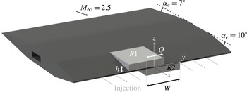
A strut injector (see figure 1), mounted in the centre plane of the supersonic wind-tunnel’s test section and spanning its entire width, was used in this work as it served as modular platform allowing for the placement of multiple ramp configurations to study the evolution and dynamics of pre-imposed vortical systems (Vergine & Maddalena Reference Vergine and Maddalena2012). When present, the injectant is delivered through a thin slit located on the symmetry plane at the trailing edge of the strut. The injection slit was designed to generate a nearly two-dimensional plume (the size of the injection port is
 $101.6\times 0.5~\text{mm}^{2}$
). The unswept expansion ramps (expansion angle
 $\unicode[STIX]{x1D6FC}_{e}=10^{\circ }$
; height at the base
 $h=5.8$
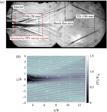
mm) were kept in place on the expansion surface of the injector through a shallow spanwise groove, carefully filled before the experiments. The presence of the strut allowed for a shock-free area between the streamwise stations located at 58 mm and 186 mm (i.e.
 $10h$
and
 $32h$
, respectively) downstream of the injection point (see the shadowgraph image in figure 2
a). In all the cases inspected in this manuscript the strut produces a wake flow in which the streamwise vortices evolve, as can be seen in figure 2(b). Note that the measured velocity magnitude exceeds that of the free stream only within the Prandtl–Meyer expansion region ahead of the recompression shocks. The slight change in the shock pattern inclination when the injector was equipped with compression–expansion ramps did not affect the surveyed stations which always remained in the shock-free region downstream, as can also be inferred by the S-PIV results shown later.
The cases of ramp configurations used in the experiments were based on the results of the simulations conducted with VorTx, which were targeted to obtain either merging or non-merging of the co-rotating vortices within two CVPs of opposite sign shed from the ramps. The reduced-order simulations are omitted in this manuscript as not part of the scope of the manuscript, however, the interested reader may consult the work of Vergine & Maddalena (Reference Vergine and Maddalena2015), where the simulations for cases I and II are shown.
The five cases presented in this work were obtained by using ramps the height of which was either
 $h$
or
 $2h$
(where
 $h=5.8$
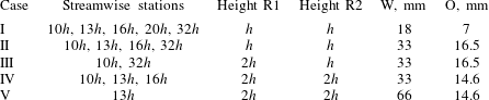
mm) with different widths W and by varying the overlap O between the internal edges of the vortex generators. All of them, except case V, were composed of four vortices arranged in two CVPs, in which the differences resided in the distance among the structures (i.e. the width of the ramps is not expected to affect the strength of the vortices). The mutual overlaps between the counter-rotating vortex pairs were 7 mm for case I, 16.5 mm for cases II and III, 14.6 mm for cases IV and V. In case V the compression ramps in use were spanning almost the entire half-width of the strut to exclude the interaction of the external vortices with the merger.
Schematic of the strut injector equipped with expansion ramps.

(a) Shadowgraph of the flow downstream of the strut; (b) streamwise PIV survey.

2.1 Stereoscopic particle image velocimetry system set-up
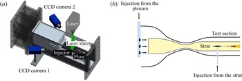
Stereoscopic particle image velocimetry was the flow measurement technique used in this investigation. The S-PIV system available consists of a double-pulsed New Wave Research Solo PIV 120 Nd:YAG laser, two LaVision Imager Intense cameras (
 $1376\times 1040~\text{px}^{2}$
, pixel size:
 $6.45~\unicode[STIX]{x03BC}\text{m}$
) equipped with 50 mm lenses and the LaVision DaVis 7.1 software used for the post-processing. The particles can be delivered through both the injection port of the strut and the injection system mounted in the supersonic wind-tunnel reservoir to seed the entire flow field. In some of the surveys (i.e. cases I and II) it was chosen to deliver particles from both locations to better mark the plume issuing from the injection port and enable plume morphology studies. To do so, a very small amount of helium (fuel-to-free stream momentum flux ratio
 $J=1\times 10^{-3}$
) was delivered through the injection slit of the strut to ensure the proper entrainment of the tracers yet limiting as much as possible the momentum added into the flow.
Figures 3(a) and 3(b) show the schematic of the PIV set-up and the seeding injection system adopted during the experiments.
Schematics of (a) the PIV system set-up used in the surveys and (b) the flow-seeding strategy adopted in the supersonic wind tunnel.

 $\text{TiO}_{2}$
nano-particles were chosen for their size and limited agglomeration (nominal diameter: 20 nm; cluster diameter:
 $0.25~\unicode[STIX]{x03BC}\text{m}$
; density:
 $4130~\text{kg}~\text{m}^{-3}$
). The assessment of the particle response downstream of a shock performed by the authors (Vergine & Maddalena Reference Vergine and Maddalena2014) confirmed that the
 $\text{TiO}_{2}$
particles can closely track the imposed vortex field.
The cameras were positioned so as to achieve approximately the same resolution in all the experiments (i.e.
 $0.06~\text{mm}~\text{px}^{-1}$
) resulting in an interrogation area (
 $32\times 32~\text{px}^{2}$
) of approximately 1.86 mm and a grid spacing of 0.93 mm due to the
 $50\,\%$
overlap among neighbouring cells. Based on the size of the interrogation area, it is possible to calculate a cutoff wavenumber
 $k_{cut}=1.69~\text{rad}~\text{mm}^{-1}$
, which must be considered the upper bound of the resolved turbulence spectrum in these measurements.
As the turbulence time scale was estimated to be
 $4~\unicode[STIX]{x03BC}\text{s}$
in this class of flows, the pulse separation time
 $\unicode[STIX]{x0394}t$
chosen for the experiments was
 $1.2~\unicode[STIX]{x03BC}\text{s}$
, to permit to freeze the motion of the fastest-decaying turbulent eddies while still allowing for measurable in-plane displacements (Vergine & Maddalena Reference Vergine and Maddalena2014). The upper bound of the pulse separation time was constrained by the necessity of keeping the out-of-plane motion around
 $1/4$
of the laser sheet thickness which, therefore, was set to its maximum nominal value of 2 mm.
Test matrix.

3 Test matrix
The nominal stagnation conditions adopted in the experiments (
 $p_{0_{\infty }}=610$
kPa,
 $T_{0_{\infty }}=294$
K) permitted steady run times of approximately 13 s each and a free stream Reynolds number per unit length of
 $6.45\times 10^{7}~\text{m}^{-1}$
. Due to the different size and strength of the streamwise structures, the vortex Reynolds numbers (i.e. the ratio between the circulation and the laminar viscosity at the free stream static temperature) ranged between
 $2.99\times 10^{5}$
and
 $8.25\times 10^{5}$
(See § 5). The location of the stations inspected in the streamwise direction is a multiple of
 $h=5.8$
mm, the height of the expansion ramps in use and chosen as a base dimension. Table 1 summarizes the test matrix indicating the streamwise stations probed and the values of ramp’s height, width and overlap employed in each inspected case. Note that in case III the height of the ramp on the top surface of the strut
 $R1$
was double that of the ramp on the bottom surface
 $R2$
.
Average S-PIV data were obtained by collecting approximately 250–900 instantaneous flow fields at the different streamwise stations. Within this range of realizations, the
 $TKE$
data reached convergence in all the probed vortices. The different number of image pairs collected were due both to experimental limitations and to the rejection of the instantaneous flow fields containing the majority of spurious vectors. Although the average quantities reached convergence for few tens of collected pairs with acceptable uncertainties, the statistical quantities might have not converged as fast. For this reason, a study of the
 $TKE$
in selected points of the flow field (i.e. the point of peak turbulent kinetic energy in each structure) was conducted.
All the results in the manuscript are normalized with the same maximum measured value of the quantity of interest. Specifically, the vorticity is normalized with the absolute value of the peak that was measured at station
 $10h$
for case I,
 $\unicode[STIX]{x1D714}_{x,ref}=5.21\times 10^{4}~\text{s}^{-1}$
, and the circulation is normalized by the absolute value of that of the merger (the largest structure in the flow field) at station
 $10h$
for case I,
 $\unicode[STIX]{x1D6E4}_{ref}=3.47~\text{m}^{2}~\text{s}^{-1}$
. The
 $TKE$
is also normalized by the maximum value obtained at station
 $10h$
for case I,
 $TKE_{ref}=3.86\times 10^{3}~\text{m}^{2}~\text{s}^{-2}$
. The spatial coordinates are normalized with respect to
 $h$
. Note that in some of the cases presented in the second part of the manuscript (i.e. case III, IV or V) the peak
 $TKE$
in the vortical structures is higher than
 $TKE_{ref}$
, thus explaining normalized values being greater than one.
As the work is focused on studying the dependence of the turbulent kinetic energy of the streamwise vortices on the vortex Reynolds number and the streamwise distance, slight changes in flow conditions downstream of the re-compression shock due to the different ramp geometries do not influence the final analysis.
4 Part I: cases I and II
4.1 Cases I and II: mean flow data
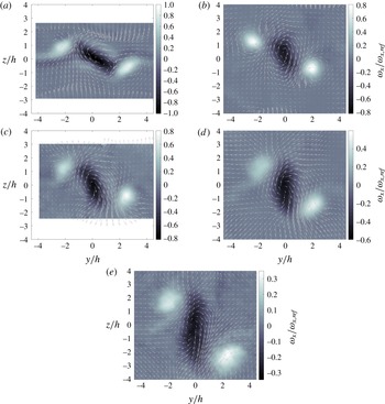
Figure 4 shows the velocity vector fields and the average streamwise vorticity contour plots normalized respect to the maximum value obtained in the S-PIV surveys conducted at station
 $10h$
,
 $\unicode[STIX]{x1D714}_{x,ref}=5.21\times 10^{4}~\text{s}^{-1}$
. The central vortices shed from the internal edges of the ramps resulted already merged at station
 $10h$
, forming an elongated vorticity patch which evolved and rotated up to station
 $32h$
, assuming a bean-like shape. By visual inspection, the size of the merger is approximately double that of the external vortices. Note that the contour plots have been re-scaled to better highlight the geometrical features of the streamwise vorticity field. A comprehensive analysis of the plume and the mean flow fields of this case can be found in Maddalena et al. (Reference Maddalena, Vergine and Crisanti2014).
Case I: evolution of the streamwise vorticity normalized by
 $\unicode[STIX]{x1D714}_{x,ref}=5.21\times 10^{4}~\text{s}^{-1}$
. Stations (a)
 $10h$
, (b)
 $13h$
, (c)
 $16h$
, (d)
 $20h$
and (e)
 $32h$
.

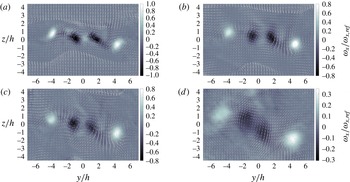
The average flow fields obtained for case II are shown in figure 5 for all the streamwise stations considered. As seen in this case, the central vortices did not fully merge throughout the entire survey and their vorticity peaks remained well separated up to station
 $32h$
.
Case II: evolution of the streamwise vorticity normalized by
 $\unicode[STIX]{x1D714}_{x,ref}=5.21\times 10^{4}~\text{s}^{-1}$
. Stations (a)
 $10h$
, (b)
 $13h$
, (c)
 $16h$
and (d)
 $32h$
.

4.2 Circulation of the vortices
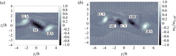
The analysis from this point will be carried out by referring to the different vorticity patches with acronyms. Images in figure 6 presents the nomenclature adopted to identify the structures in the two cases inspected. Specifically: ELV and ERV indicate the external-left vortex and external-right vortex, respectively; ML and MR stand for median-left and median-right vortices; M indicates the merger.
Nomenclature of the structures in the flow fields: (a) case I; (b) case II. The streamwise vorticity contour is shown normalized by
 $\unicode[STIX]{x1D714}_{x,ref}=5.21\times 10^{4}~\text{s}^{-1}$
.

Note that the presentation of the results in this manuscript slightly differs from that provided by Vergine & Maddalena (Reference Vergine and Maddalena2015) due to: (i) updated datasets for the
 $13h$
station of case I and the
 $10h$
station of case II and (ii) the addition of the
 $13h$
station in case II.
The circulation of the structures was evaluated as the flux of streamwise vorticity which was above its maximum statistical uncertainty among all the surveyed stations, in this case
 $\pm 5000~\text{s}^{-1}$
(i.e. less than
 $10\,\%$
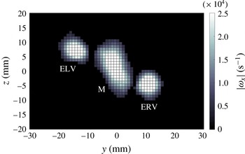
of the maximum measured value). In figure 7 the actual cells over which the streamwise vorticity was averaged are presented for each structure for case I, station
 $13h$
: a location where the vorticity patches lay in close proximity. In this way, only the vorticity that can be confidently measured contributes to the calculation of the circulation. Note that the area used to evaluate the circulation coincides with the area over which the
 $TKE$
is averaged in the calculation of
 $TKE_{AVG}$
.
Case I, station
 $13h$
. Streamwise vorticity magnitude exceeding
 $5000~\text{s}^{-1}$
.

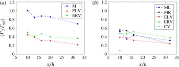
Figures 8(a) and 8(b) present the evolution of the circulation of each structure calculated as the flux of streamwise vorticity across the patch and normalized with respect to
 $\unicode[STIX]{x1D6E4}_{ref}$
for case I and case II, respectively. It is noteworthy that the circulation of the merger in case I is essentially double that of the external structures, while the circulation is quite similar for all the vortices in case II.
The measurement error on each velocity component
 $e_{v}$
is evaluated as the combination of the systematic interpolation error
 $e_{s}$
and the random error
 $e_{rand}$
affecting the measured in-plane velocity components:
 $e_{v}=\sqrt{e_{s}^{2}+e_{rand}^{2}}$
. The systematic error
 $e_{s}$
is here made to coincide with the intrinsic uncertainty given by the use of a three-point Gaussian interpolator for the evaluation of the fractional displacement within the interrogation area and typically of the order of one-tenth of a pixel. This error has been estimated to be
 $\pm 4.8~\text{m}~\text{s}^{-1}$
for the experimental conditions attained. Although the random error
 $e_{rand}$
is usually very small, its evaluation in each interrogation area was necessary due to its strong dependence on the seeding density which could not necessarily be the same in every realization. The analysis of the random error allowed us to consider a maximum of
 $\pm 1.5~\text{m}~\text{s}^{-1}$
, which was assumed constant to produce conservative estimates. The total error on the measurement of each velocity component is, therefore,
 $e_{v}=5~\text{m}~\text{s}^{-1}$
. The error on the circulation can be evaluated as follows (4.1):
 $$\begin{eqnarray}e_{\unicode[STIX]{x1D6E4}}=\sqrt{\sum (e_{\unicode[STIX]{x1D714}_{x}}A_{i})^{2}}.\end{eqnarray}$$
Where the summation is taken across the area occupied by the streamwise vorticity of each structure above the cutoff,
 $e_{\unicode[STIX]{x1D714}_{x}}=2\sqrt{e_{s}^{2}+e_{rand}^{2}}$
is the error on the streamwise vorticity (i.e. twice as much as
 $e_{v}$
) and
 $A_{i}$
is the area of the
 $i$
th cell. Although the error on the velocity components is measurable, that on the circulation resulted always of the order of
 $10^{-4}~\text{m}^{2}~\text{s}^{-1}$
for each vorticity patch and, therefore, negligible.
Circulation of the vortices along the probed flow field. (a) Case I and (b) case II. The values are normalized by
 $\unicode[STIX]{x1D6E4}_{ref}=3.47~\text{m}^{2}~\text{s}^{-1}$
.

4.3 Fluctuating flow measurements: methodology, convergence and uncertainty
Single point values of the
 $TKE$
are calculated in the location of its peak within the vorticity patches. On the other hand, area-averaged values of the
 $TKE$
are calculated by means of the following equation:
 $$\begin{eqnarray}TKE_{AVG}=\frac{1}{A}\sum TKE_{i}A_{i},\end{eqnarray}$$
where
 $A$
is the area of the vorticity patch remaining above the chosen cutoff and
 $TKE_{i}$
is the turbulent kinetic energy. The average
 $TKE$
content across the vorticity patch is in this work a quantity of interest as it is less prone to be affected by possible inexact single-point measurements.
The
 $TKE$
is calculated as half the sum of the squares of the velocity fluctuations in the three directions across the entire range of instantaneous flow fields (4.3), namely:
 $$\begin{eqnarray}TKE={\textstyle \frac{1}{2}}(\langle {u^{\prime }}^{2}\rangle +\langle {v^{\prime }}^{2}\rangle +\langle {w^{\prime }}^{2}\rangle ).\end{eqnarray}$$
Each term in (4.3), in turn, is affected by statistical uncertainty
 $\unicode[STIX]{x1D716}_{stat}$
, due to the limited number of instantaneous flow fields collected, and a convergence error which was found negligible for the cases presented here.
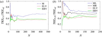
To assess the degree of convergence of the data, the peak
 $TKE$
variation with the number of realizations
 $N$
was analysed. The same steps were repeated for all the surveyed stations, however, figure 9 only shows the
 $TKE_{P}$
against
 $N$
at stations
 $16h$
for both cases I and II and which, for different reasons, could have been seriously affected by convergence problems. In fact, in case I the only meaningful portion of the aforementioned measurement was limited to the plume (due to seeding from the injector only), while in case II only a limited number of realizations could be available. All the results were declared converged if the per cent
 $TKE$
change respect to the measured final value against the number of realizations was within
 $\pm 1\,\%$
.
Peak
 $TKE$
trends with the number of realizations of the structures present in the flow field at station
 $16h$
. (a) Case I and (b) case II.

Because of the negligible convergence error, the total uncertainty on the turbulent kinetic energy can be calculated as follows in (4.4)
 $$\begin{eqnarray}\unicode[STIX]{x1D6FF}TKE={\textstyle \frac{1}{2}}\sqrt{(\unicode[STIX]{x1D716}_{stat,\langle {u^{\prime }}^{2}\rangle }^{2})^{2}+(\unicode[STIX]{x1D716}_{stat,\langle {v^{\prime }}^{2}\rangle }^{2})^{2}+(\unicode[STIX]{x1D716}_{stat,\langle {w^{\prime }}^{2}\rangle }^{2})^{2}}.\end{eqnarray}$$
The statistical uncertainty
 $\unicode[STIX]{x1D716}_{stat}$
depends on the fourth and the second statistical moments along with the number of realizations collected in each point and it is evaluated for a
 $95\,\%$
confidence interval (Benedict & Gould Reference Benedict and Gould1996). Specifically, for one of the squares of the fluctuating components of the velocity (namely,
 $\langle {u^{\prime }}^{2}\rangle$
), the statistical error can be written as:
 $$\begin{eqnarray}\unicode[STIX]{x1D716}_{stat,\langle {u^{\prime }}^{2}\rangle }=1.96\sqrt{\frac{\langle {u^{\prime }}^{4}\rangle -\langle {u^{\prime }}^{2}\rangle ^{2}}{N}}.\end{eqnarray}$$
Where
 $N$
is the number of realization in each point of the flow field.
The magnitude of each velocity fluctuation and the fluctuating component of the streamwise vorticity will be extracted from the point of peak
 $TKE$
to understand their relative contribution. For the uncertainty on the single fluctuations (i.e. velocity and vorticity) the formulation in (4.6) was used. Note that (4.6) is written for the streamwise velocity fluctuations, but can be applied to the remaining components as well as to the fluctuating vorticity by substituting the respective statistical moments:
 $$\begin{eqnarray}\unicode[STIX]{x1D716}_{stat,\langle {u^{\prime }}^{2}\rangle ^{0.5}}=1.96\sqrt{\frac{1}{N}\frac{\langle {u^{\prime }}^{4}\rangle -\langle {u^{\prime }}^{2}\rangle ^{2}}{4\langle {u^{\prime }}^{2}\rangle }}.\end{eqnarray}$$
The error on the
 $TKE$
measurement is overlapped to the statistical uncertainty. The aforementioned error depends on the square of the fluctuations in the interpolation error
 $\langle e_{s}\rangle ^{2}$
introduced by the peak-detection algorithm employed by the PIV software (see § 4.2) and on the square of the fluctuations in the random error
 $\langle e_{rand}\rangle ^{2}$
. In this case, the respective contributions of the aforementioned errors were found to be approximately
 $\langle e_{s}\rangle ^{2}=23~\text{m}^{2}~\text{s}^{-2}$
and
 $\langle e_{rand}\rangle ^{2}=0.4~\text{m}^{2}~\text{s}^{-2}$
, therefore, negligible for the
 $TKE$
values presented in this manuscript.
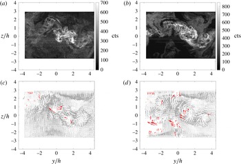
Case I, station
 $10h$
. (a,b) Instantaneous images from one of the PIV cameras in use; (c,d) instantaneous flow fields resulting from the same shots.

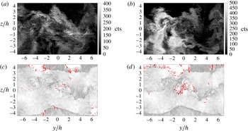
In order to show the quality of the recorded images (see figures 10
a,b and 11
a,b) and the number of valid the realizations contributing to both data and uncertainty, two representative instantaneous flow fields were extracted from the data collected at station
 $10h$
for case I (figure 10
c,d) and at station
 $13h$
for case II (figure 11
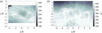
c,d), respectively. The selected locations represent worst cases scenarios as they could be poisoned with reflections and uneven seeding which often result in lack of correlation and, therefore, an empty space in the PIV grid. The two instantaneous flow fields have been chosen to show a typical realization with an almost full vector field and another with fewer vectors.
Case II, station
 $13h$
. (a,b) Instantaneous images from one of the PIV cameras in use; (c,d) instantaneous flow fields resulting from the same shots.

Grey vectors in figures 10 and 11 represent the valid realizations calculated by means of the PIV software in use (DaVis 7.1). The software was set-up to remove as many spurious vectors as possible from each instantaneous flow field and attempting to keep the largest number of ‘good’ vectors. However, after visual inspection, a few invalid vectors were still present and an internally developed post-processing code was used to apply a median filter for the removal of the remaining false vectors, which were highlighted in red in figures 10 and 11. Note that the median filter compares the in-plane magnitude of a velocity vector with the mean of its neighbours and eliminates it if the per cent difference is above
 $75\,\%$
. As can be seen, empty spots were present in the measurements, however, they are mostly confined outside the area of interest in all the instantaneous realizations.
Although any median filter inevitably removes also good vectors, the benefit of getting rid of spurious data largely overcomes the negative effect of removing good data. Figures 12(a) and 12(b) show the total amount of valid realizations
 $N$
per spatial location; although a slight lack of data is present within the central vorticity patch for case I (much milder is the loss of data in case II), the amount of realizations was still sufficient to attain convergence of the results.
Number of realizations per point. (a) Case I, station
 $10h$
; (b) case II, station
 $13h$
.

4.4 Case I: fluctuating flow data
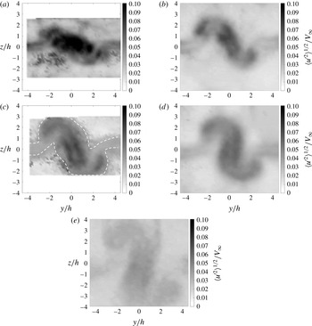
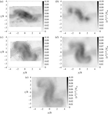
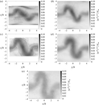
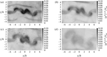
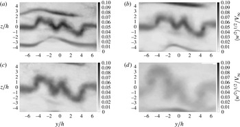
Figures 13–15 present the fluctuating components of the velocity across the flow fields for case I, normalized by the nominal free stream velocity (i.e.
 $V_{\infty }=572.89~\text{m}~\text{s}^{-1}$
). As can be seen, the magnitude of the velocity fluctuations remains of the order of one-tenth of
 $V_{\infty }$
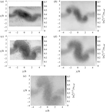
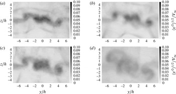
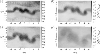
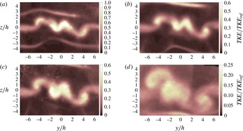
all along the surveyed flow field. The image in figure 16 shows the normalized fluctuating component of the streamwise vorticity: turbulence imposes a very large fluctuation of the aforementioned quantity, especially inside the vorticity patches where it is actually comparable with its peak value. Finally, figure 17 shows the
 $TKE$
– normalized by
 $TKE_{ref}=3.86\times 10^{3}~\text{m}^{2}~\text{s}^{-2}$
– as calculated by means of (4.3) at the different stations. Note that the measurement at station
 $16h$
was originally conducted by seeding the injectant only; therefore, the abrupt variation of the aforementioned quantities between the wake and the external flow is an artefact of the data reduction code due to the different number of valid realizations in those areas. The data that should be considered valid are those within the dashed line only.
Case I: evolution of the fluctuating component of the streamwise velocity normalized by
 $V_{\infty }=572.89~\text{m}~\text{s}^{-1}$
. Stations (a)
 $10h$
, (b)
 $13h$
, (c)
 $16h$
, (d)
 $20h$
and (e)
 $32h$
.

Case I: evolution of the fluctuating component of the velocity along the
 $y$
axis normalized by
 $V_{\infty }=572.89~\text{m}~\text{s}^{-1}$
. Stations (a)
 $10h$
, (b)
 $13h$
, (c)
 $16h$
, (d)
 $20h$
and (e)
 $32h$
.

Case I: evolution of the fluctuating component of the velocity along the
 $z$
axis normalized by
 $V_{\infty }=572.89~\text{m}~\text{s}^{-1}$
. Stations (a)
 $10h$
, (b)
 $13h$
, (c)
 $16h$
, (d)
 $20h$
and (e)
 $32h$
.

Case I: evolution of the fluctuating component of the streamwise vorticity normalized by
 $\unicode[STIX]{x1D714}_{x,ref}=5.21\times 10^{4}~\text{s}^{-1}$
. Stations (a)
 $10h$
, (b)
 $13h$
, (c)
 $16h$
, (d)
 $20h$
and (e)
 $32h$
.

Case I: evolution of the
 $TKE$
normalized by
 $TKE_{ref}=3.86\times 10^{3}~\text{m}^{2}~\text{s}^{-2}$
. Stations (a)
 $10h$
, (b)
 $13h$
, (c)
 $16h$
, (d)
 $20h$
and (e)
 $32h$
.

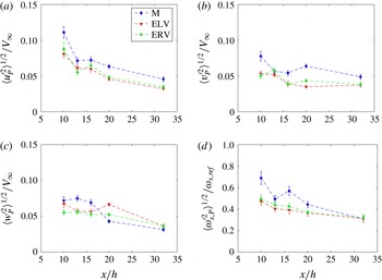
The plots in figure 18 show the trends of the fluctuating components of the velocity (figure 18
a–c) and the vorticity (figure 18
d) in the point where the turbulent kinetic energy of each structure reaches a peak. The first main difference between them is the magnitude recorded in the closest streamwise station (i.e.
 $10h$
): it appears that the axial fluctuations in that location are approximately double those along
 $y$
and
 $z$
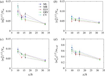
for each structure, with higher values in the merger when compared with the external vorticity patches. Additionally, the decay of the in-plane fluctuations is much slower than that in the streamwise direction, suggesting that the strong large-scale stirring motion of the vortices is sustaining them. On the other hand, the fluctuations of the streamwise velocity component measurably decrease, being, therefore, the main cause of the turbulence decay shown in figure 19. As far as the vorticity fluctuations, it is noteworthy that they remain always comparable with the mean peak vorticity (the weaker fluctuations in the point of maximum turbulence at
 $32h$
are still 35 %–40 % of
 $\unicode[STIX]{x1D714}_{x,ref}$
) but, similarly to the other fluctuating quantities, seem to increase with the strength and the size of the structures.
Case I: trends of the normalized fluctuating components of (a) the streamwise velocity, (b) the
 $y$
-component of the velocity, (c) the
 $z$
-component of the velocity and (d) the streamwise vorticity in the point of peak
 $TKE$
.

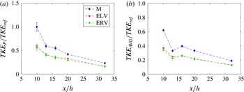
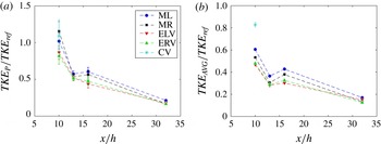
Figure 19(a,b) show the evolution of the normalized peak
 $TKE$
(denoted by the subscript
 $P$
) and that of the average
 $TKE$
(i.e.
 $TKE_{AVG}$
) across each vortex, respectively. As might be expected due to the large number of cells constituting the vorticity patch, the total error for
 $TKE_{AVG}$
is so much smaller than that attained in the single point measurement of
 $TKE_{P}$
that the error bars are almost completely absent.
Case I: trends of
 $TKE$
normalized by
 $TKE_{ref}=3.86\times 10^{3}~\text{m}^{2}~\text{s}^{-2}$
along the streamwise direction. (a) Peak
 $TKE$
and (b) average
 $TKE$
across the vorticity patch.

There are two important considerations to be made based on the plots shown in figure 19: (i) the intensity of the
 $TKE$
(both peak and average) in the merger is very close to being double that of the isolated vortices at stations
 $10h$
and
 $13h$
and (ii)
 $TKE$
is still being produced between stations
 $10h$
and
 $20h$
. Regardless of the uncertainty, in fact, a clear inversion of the trend of the curves in each patch is noticeable, thus suggesting that the
 $TKE$
production overcame its decay at station
 $16h$
, especially when the average taken across the mean streamwise vorticity patch is considered.
The first, in particular, is notable result in light of the fact that it is legitimate to assume – at least in the absence of vortex stretching phenomena – that the initial values of the fluctuating components of the vortices should have been the same for all the structures before merging took place, as will also be shown for case II. Therefore, these measurements seem to suggest the presence of a proportionality law between circulation and
 $TKE$
, de facto linking mean and fluctuating flow fields.
4.5 Case II: fluctuating flow data
Figures 20–23 show the normalized fluctuating components of the velocity and the streamwise vorticity across the flow field imposed by the vortical structures present in case II. Even for this non-merging scenario, the magnitude of the fluctuations remains of the order of one tenth of the free stream velocity all along the surveyed flow field (see figures 20–22), although the spatial distribution of the fluctuations is very different from those of case I (compare with figures 13–15). Also, the morphology of the normalized
 $TKE$
scalar field, presented in figure 24, is much different from that of the merging case in figure 17. Compared to case I, where the merger induced a rotation in the clockwise direction of both the whole system of vortices and the
 $TKE$
scalar field, the structures in this case do not rotate around a common centre, thus preventing the redistribution of the turbulent kinetic energy in the direction of rotation. The only notable similarity with case I are the turbulence levels which are not too different and can be presented with the same scale. The major modification that the flow field undergoes is due to diffusion and the natural turbulence decay noticeable at downstream stations.
Case II: evolution of the fluctuating component of the streamwise velocity normalized by
 $V_{\infty }=572.89~\text{m}~\text{s}^{-1}$
. Stations (a)
 $10h$
, (b)
 $13h$
, (c)
 $16h$
and (d)
 $32h$
.

Case II: evolution of the fluctuating component of the velocity along the
 $y$
axis normalized by
 $V_{\infty }=572.89~\text{m}~\text{s}^{-1}$
. Stations (a)
 $10h$
, (b)
 $13h$
, (c)
 $16h$
and (d)
 $32h$
.

Case II: evolution of the fluctuating component of the velocity along the
 $z$
axis normalized by
 $V_{\infty }=572.89~\text{m}~\text{s}^{-1}$
. Stations (a)
 $10h$
, (b)
 $13h$
, (c)
 $16h$
and (d)
 $32h$
.

Case II: evolution of the fluctuating component of the streamwise vorticity normalized by
 $\unicode[STIX]{x1D714}_{x,ref}=5.21\times 10^{4}~\text{s}^{-1}$
. Stations (a)
 $10h$
, (b)
 $13h$
, (c)
 $16h$
and (d)
 $32h$
.

Case II: evolution of the
 $TKE$
normalized by
 $TKE_{ref}=3.86\times 10^{3}~\text{m}^{2}~\text{s}^{-2}$
. Stations (a)
 $10h$
, (b)
 $13h$
, (c)
 $16h$
and (d)
 $32h$
.

Figure 25 shows the trends of the fluctuating components of the velocity and streamwise vorticity in the point of peak turbulence. Also in the non-merging scenario, the fluctuations along the
 $y$
and
 $z$
axes not only are not as strong as those along
 $x$
, but their decay proceeds in a slower fashion for every vorticity patch from which they have been extracted. In this case, however, the levels of the fluctuations do not differ much although higher values are extracted from the middle patches (i.e. ML, MR and CV), attesting the presence of an area in which the very large shear due to the close vicinity of strong co-rotating vortices contributes to produce turbulence. The vorticity fluctuations, on the other hand, seem to decay in a very similar way for each vortex and, analogously with the findings of case I, their magnitude remains always comparable to
 $\unicode[STIX]{x1D714}_{x,ref}$
.
Case II: trends of the normalized fluctuating components of (a) the streamwise velocity, (b) the
 $y$
-component of the velocity, (c) the
 $z$
-component of the velocity and (d) the streamwise vorticity in the point of peak
 $TKE$
.

As can be seen in the plots of figure 26, the intensities of the
 $TKE$
are very similar for each structure at each streamwise station, with slightly higher values in the central vorticity patches. This result builds on the findings presented in § 4.4, where it was postulated that the peak
 $TKE$
may scale with the vortex’s size and strength. Interestingly, this is not the case for the central vorticity patch which is characterized by fairly low circulation, a very large value of peak
 $TKE$
, and which is not a structure generated by the ramps. Also in this case, a measurable inversion of the
 $TKE$
trend (both peak and average) can be recognized between
 $10h$
and
 $16h$
, indicating that turbulence production overcomes the decay in this area.
Case II: trends of
 $TKE$
normalized by
 $TKE_{ref}=3.86\times 10^{3}~\text{m}^{2}~\text{s}^{-2}$
along the streamwise direction. (a) Peak
 $TKE$
and (b) average
 $TKE$
across the vorticity patch.

5 Part II: turbulence characterization and dimensional analysis
5.1 Cases III–V: mean and fluctuating flow data
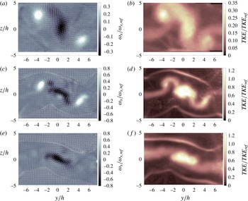
Figure 27 shows the normalized streamwise vorticity and the
 $TKE$
for cases III–V at selected streamwise stations to show the wide variety of streamwise vorticity and turbulent kinetic energy distributions possible with just a slight change in the mutual distance of the ramps in use. Although additional stations were probed for these cases, they are not shown as this section is mainly focused on the extraction of vortex Reynolds numbers as well as peak and average values of the turbulent kinetic energy.
The vortices shed from the internal edges of the ramps merged in all these additional cases to create a structure whose strength was roughly the sum of the circulation of the isolated ones. It is exactly this amalgamation of streamwise vorticity that enabled the study of the evolution of many different categories of supersonic vortical structures, as the merger has actually been considered a single, isolated large vortex in the following calculations.
As the
 $TKE$
contour plots show, the stronger shock generated by the taller ramps (see the contours corresponding to case IV and V in figure 27) did not noticeably change the background turbulence levels in the shock-free region in which the streamwise vortices evolve (approximately
 $150{-}200~\text{m}^{2}~\text{s}^{-2}$
in cases I–IV, while
 $250~\text{m}^{2}~\text{s}^{-2}$
in case V).
Streamwise vorticity normalized by
 $\unicode[STIX]{x1D714}_{x,ref}=5.21\times 10^{4}~\text{s}^{-1}$
(a,c,e) and
 $TKE$
normalized by
 $TKE_{ref}=3.86\times 10^{3}~\text{m}^{2}~\text{s}^{-2}$
(b,d,f) contours for (a,b) case III, station
 $32h$
; (c,d) case IV, station
 $13h$
; (e,f) case V, station
 $13h$
.

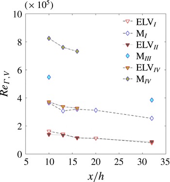
The plot in figure 28 shows the vortex Reynolds number evolution of some of the structures (i.e. the isolated vortices and the merger) along the probed flow field for the cases considered here; data from other cases have been omitted but it was verified that the same conclusions apply to all the vortices considered. A decay can be inferred in all the cases, although marginal when compared to the actual values of the Reynolds numbers attained.
Vortex Reynolds numbers of some of the structures surveyed in cases I–IV.

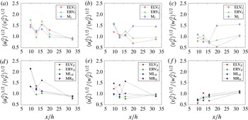
Ratios between the fluctuating velocity components: (a,d)
 $\sqrt{\langle u_{P}^{\prime 2}\rangle /\langle v_{P}^{\prime 2}\rangle }$
, (b,e)
 $\sqrt{\langle u_{P}^{\prime 2}\rangle /\langle w_{P}^{\prime 2}\rangle }$
and (c,f)
 $\sqrt{\langle v_{P}^{\prime 2}\rangle /\langle w_{P}^{\prime 2}\rangle }$
. Note that panels (a,b,c) pertain to case I, while (d,e,f) pertain to case II.

5.2 Turbulence characterization
In order to characterize the turbulence, three properties have been analysed: homogeneity, isotropy and compressibility.
The
 $TKE$
contour plots shown in figures 17, 24 and 27 clearly show the high inhomogeneity of the turbulence under consideration, highlighting how the streamwise structures act not only to produce, but also to transport, turbulence from one region to another in space.
The degree of isotropy of the turbulence was analysed in the point of peak
 $TKE$
for cases I and II (see figure 29). In case I the ratios between the fluctuations of the components of the velocity seem to lie close to 1 (i.e. local isotropic turbulence), essentially all along the flow field within the external vortices (ELV and ERV), while noticeable differences between the remaining ratios can be noticed in the merger. Especially
 $u^{\prime }/w^{\prime }$
and
 $v^{\prime }/w^{\prime }$
in the merger tend to reach a constant value of approximately 1.5 downstream. A situation which is similar to that of the external vortices of case I can be recognized in the same structures of case II, where all the fluctuating components in the point of peak turbulence tend to equalize downstream. The internal vortices (ML and MR), on the other hand, present a much more erratic behaviour, showing relatively high peaks of the quantities
 $u^{\prime }/v^{\prime }$
and
 $u^{\prime }/w^{\prime }$
at stations
 $10h$
and
 $16h$
. The non-isotropic nature of the turbulence in the same point has been verified for the whole set of cases analysed in the manuscript although the corresponding plots have been omitted.
The magnitude of the fluctuating velocity was used to estimate the fluctuating Mach number in order to discover whether or not the turbulence can be considered incompressible. It stayed below 0.3 across the probed sections remaining, therefore, within the incompressible regime.
For this reason, the data under consideration belong to an incompressible, non-homogeneous and globally anisotropic turbulence, at least in the single point corresponding to the location of the peak turbulence.
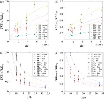
 $TKE$
peak (a,c) and average (b,d) – normalized by
 $TKE_{ref}=3.86\times 10^{3}~\text{m}^{2}~\text{s}^{-2}$
– of some of the structures as a function of (a,b) the vortex Reynolds number at different stations and (c,d) the normalized streamwise distance for different inspected cases.

5.3 Dimensional analysis
The preliminary observation of the multiple turbulence data allowed us to infer that turbulent kinetic energy, both peak and average, increases with the increasing strength of the streamwise structures (i.e. circulation) and, as expected, decays with the streamwise distance
 $x$
originating at the injection point (see figure 30). For this reason, the functional relationship between the
 $TKE$
and the aforementioned parameters is postulated to be in the form shown in (5.1)
 $$\begin{eqnarray}\unicode[STIX]{x1D713}\left(TKE,V_{\infty },\unicode[STIX]{x1D6E4},\unicode[STIX]{x1D708},\frac{x}{h}\right)=0.\end{eqnarray}$$
Assuming valid the relation in (5.1), three non-dimensional groups that regulate the phenomenon can be retrieved, specifically:
 $\unicode[STIX]{x1D6F1}_{1}=TKE/V_{\infty }^{2}$
,
 $\unicode[STIX]{x1D6F1}_{2}=\unicode[STIX]{x1D708}/\unicode[STIX]{x1D6E4}$
and
 $\unicode[STIX]{x1D6F1}_{3}=x/h$
; note that the group
 $\unicode[STIX]{x1D6F1}_{2}$
is the inverse of the vortex Reynolds number of each structure.
Equation (5.2) shows the form of the final equation relating the dimensionless parameters. In the relation,
 $\unicode[STIX]{x1D6F1}_{2}$
has been inverted to explicitly show the dependence on the vortex Reynolds number,
 $Re_{\unicode[STIX]{x1D6E4}}$
 $$\begin{eqnarray}\frac{TKE}{V_{\infty }^{2}}=CRe_{\unicode[STIX]{x1D6E4}}^{A}\left(\frac{x}{h}\right)^{B}.\end{eqnarray}$$
A constant Reynolds number to assign to each structure was needed to carry out the dimensional analysis calculations. For this purpose, the Reynolds number of each structure evaluated at the closest possible station per case inspected was assigned (i.e. considering the circulation at station
 $10h$
for cases I to IV and the circulation at
 $13h$
for case V).
Figures 30(a) and 30(b) show, respectively, the normalized peak and average
 $TKE$
as a function of
 $Re_{\unicode[STIX]{x1D6E4}}$
, measured at different stations. Figures 30(c) and 30(d) show the change in normalized peak and average
 $TKE$
as a function of the downstream distance normalized by the ramp’s height
 $h=5.8$
mm. Recall that the average
 $TKE$
is necessarily lower than the peak
 $TKE$
due to the averaging process applied to calculate it. Note that in figure 30 simple curve fits of the type:
 $y=a(x-b)^{n}$
have been included only to highlight possible qualitative trends of the turbulent kinetic energy with the vortex Reynolds number and the normalized streamwise coordinate. Specifically, the exponent
 $n=0.5$
was used to fit (
 $Re_{\unicode[STIX]{x1D6E4}},TKE/TKE_{ref}$
), while
 $n=-1$
for (
 $x/h,TKE/TKE_{ref}$
); as will be shown later these exponents are quite close to the optimal
 $A$
and
 $B$
coefficients in (5.2) calculated through dimensional analysis.
Figures 30(a,b) and 30(c,d) clearly show that the
 $TKE$
increases with increasing vortex Reynolds numbers and decays with the streamwise distance. Furthermore, very similar trends exist for both
 $TKE_{P}$
and
 $TKE_{AVG}$
, thus indicating that all the points belonging to the vortices behave in a similar manner. However, as the trends of cases I and II show some production of
 $TKE$
still occurring between
 $10h$
and
 $16h$
, the data belonging to this interval in these two cases have been neglected as we are interested in describing the turbulence decay only. In any case, a calculation performed utilizing the entire set of data (i.e. including those neglected in this work) has shown a minimal sensitivity of the final relation to the presence of this ‘production zone’ likely due to its mild nature.
To find the aforementioned relation, an optimization algorithm calculates the best combination of
 $A$
and
 $B$
to yield the highest coefficient of determination of the linear fit
 $R^{2}$
between
 $TKE/V_{\infty }^{2}$
and
 $Re_{\unicode[STIX]{x1D6E4}}^{A}\left(x/h\right)^{B}$
. The peak in the map of coefficients
 $R^{2}=f(A,B)$
corresponds to the optimal combination of
 $A$
and
 $B$
. Based on the analysis of the trends obtained from experimental results, the calculation was performed assuming a range of
 $B$
coefficients between 0 and
 $-3$
, and a range between 0 and 3 for the
 $A$
coefficients.
The corresponding maximum
 $R^{2}$
is 0.97 for the correlation involving
 $TKE_{P}$
, with the optimal combination of coefficients being:
 $A=0.48$
and
 $B=-1.38$
. The
 $R^{2}$
is instead 0.93 for the correlation on
 $TKE_{AVG}$
, with corresponding coefficients:
 $A=0.48$
and
 $B=-1.35$
.
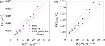
By plotting the experimental data combined as in the right-hand side of (5.2), the coefficient
 $C$
in (5.2) can be retrieved by means of a simple linear fit of the data (see 31). The fits in 31 (solid line) include the
 $95\,\%$
confidence bounds (the dashed lines), indicating that the
 $95\,\%$
of future realizations are expected to be included in that range. Note that although all the data come from vortices produced and evolving in different ways (i.e. some are shed from the ramps some other are mergers), they all closely follow the proposed power laws. Therefore, the relationships cannot be used to explain how the vortices are formed or evolve, an information that only the analysis of their interaction can provide.
Correlations and fits for (a) peak
 $TKE$
and (b) average
 $TKE$
.

The final functional relationships (i.e. the slope of the solid line in figure 31) that describe the decay of the peak and average
 $TKE$
across the vortices are presented in (5.3) and (5.4)
 $$\begin{eqnarray}\displaystyle \frac{TKE_{P}}{V_{\infty }^{2}}=2.67\times 10^{-7}\left[Re_{\unicode[STIX]{x1D6E4}}^{0.48}\left(\frac{x}{h}\right)^{-1.38}\right]+1.38\times 10^{-3} & & \displaystyle\end{eqnarray}$$
 $$\begin{eqnarray}\displaystyle \frac{TKE_{AVG}}{V_{\infty }^{2}}=1.31\times 10^{-7}\left[Re_{\unicode[STIX]{x1D6E4}}^{0.48}\left(\frac{x}{h}\right)^{-1.35}\right]+1.47\times 10^{-3}. & & \displaystyle\end{eqnarray}$$
At first glance, equation (5.2) is similar to the relation for the grid turbulence decay in (1.3) and reworked in the form given in (5.5)
 $$\begin{eqnarray}\frac{TKE}{V_{\infty }^{2}}=\left(\frac{\unicode[STIX]{x1D708}}{\unicode[STIX]{x1D706}V_{\infty }}\right)^{2}Re_{0}\left(\frac{x-x_{0}}{L_{B}}\right)^{m-(n/2)}.\end{eqnarray}$$
Particularly, when the vortex Reynolds number is taken in the place of the grid Reynolds number the structure of the equations is the same. Although the data presented § 4 clearly showed a non-isotropic nature of the turbulence under consideration, the inspection of the fluctuating Mach numbers across each flow field did reveal that the turbulence considered here is essentially incompressible in nature, thus partially justifying the aforementioned similarity.
The differences between the isotropic incompressible turbulence and that introduced by the streamwise vortices under consideration are noteworthy. By considering
 $\left(\unicode[STIX]{x1D708}/\unicode[STIX]{x1D706}V_{\infty }\right)^{2}$
a constant, the exponent corresponding to
 $A$
in (5.5) is 1, while that corresponding to
 $B$
is
 $-0.275$
; in fact,
 $m=0.35$
and
 $n=1.25$
for grid turbulence (Valente & Vassilicos Reference Valente and Vassilicos2011). This indicates that in the subsonic, isotropic turbulence a stronger dependence of the
 $TKE$
on the Reynolds number and a much slower decay is found when compared to the turbulence data provided in this manuscript.
6 Conclusions
An experimental campaign was conducted in a Mach 2.5 flow to study the decay of turbulence in complex flows originating from a five cases of supersonic streamwise vortex interaction.
In the first part of the manuscript the detailed analysis of the turbulence was presented for a case where the resulting vortex dynamics evolves in the vortex merging of two co-rotating structures in the flow field (case I) and a case where the merging process is avoided (case II). The fluctuating components in the measurements were extracted from the point where the
 $TKE$
peaks within each vorticity patch and their decay along the flow field was quantified and analysed for cases I and II. The
 $TKE$
decay was also presented considering its area-averaged value across the vorticity patches.
Because of the possible repercussions of the aforementioned
 $TKE$
scaling with the size and strength of a supersonic streamwise vortex both in the validation of CFD models and in the design of scramjet injection concepts, the second part of the manuscript was aimed at experimentally substantiate the results of the analysis conducted for cases I and II with the addition of data from three more cases (i.e. cases III–V). The relatively large amount of data collected resulted sufficient to find a suitable scaling law of the turbulence decay in these vortical flows through the application of dimensional analysis.
The main conclusions that can be drawn from this study are the following:
-
(i) In case I (i.e. the merging case) the streamwise velocity and vorticity fluctuations as well as the
 $TKE$
in the merged patch are almost double those in the isolated structures.
-
(ii) In case II (i.e. the non-merging case) the intensities of the fluctuating components (including streamwise vorticity and
$TKE$
) were very similar for each structure at each streamwise station. -
(iii) It was identified that
$TKE$
, both local and average, invert their decay between
$10h$
and
$20h$
in cases I and II. This is potentially beneficial in the design of streamwise vortex-based injection strategies for scramjets, as it suggests that it may be possible to target pre-determined shifts of the ‘turbulence production zone’ through specific vortex interactions. -
(iv) The measurements presented in part I of the manuscript suggested that the turbulent kinetic energy content in the vortices increases in structures characterized by higher circulation, thus suggesting a possible scaling between the aforementioned quantities and providing fundamental grounds for the study presented in part II.
-
(v) In part II the peak and the area-averaged
$TKE$
(i.e.
$TKE_{P}$
and
$TKE_{AVG}$
) were related to the vortex Reynolds number
$Re_{\unicode[STIX]{x1D6E4}}$
and the normalized streamwise distance
$x/h$
, and showed recognizable trends for all the inspected cases. The
$TKE$
content in the structures was found to increase with the vortex Reynolds number while decaying as expected with the streamwise distance. -
(vi) Dimensional analysis was used to find semi-empirical power laws correlating
$TKE$
,
$x/h$
and
$Re_{\unicode[STIX]{x1D6E4}}$
with high coefficients of determination. It was found that the form of the resulting law describing the
$TKE$
decay within the various interacting vortical structures is similar, in its mathematical formulation, to that of incompressible homogeneous and isotropic turbulence, but is characterized by quite different decay exponents.


Due to the dependence of the
 $TKE$
production on the mean flow strain rates (see (1.2)), which are directly affected by the strength, the position and the dynamics of the streamwise vortical structures introduced in the flow field as discussed in the experiments presented in this manuscript, it is possible to conjecture that specifically designed vortex interactions can be tailored to enhance strain rates and turbulence in targeted locations within the flow. As shown in (1.1), mixing rates are affected by both strain rates at the interface between the components of the mixture and the binary turbulent diffusion coefficient. Thus, this work shows that a deeper understanding of the vortex dynamics in supersonic flows and associated turbulence transport can have a profound impact in the definition of efficient mixing configurations, and more work on this area is recommended.
Acknowledgement
This research was sponsored (in part) by the NASA Langley Research Center through the NASA Research Announcement grant number NNX12AG46A with Dr T. G. Drozda as the Technical Monitor.