1 Introduction
The most common issue in multi-agent reinforcement learning (MARL) is the exponential increase of the state space with each additional agent. Alternatively, agents could observe only local state information, but due to the lack of observability of the other agents, the world then appears non-deterministic to each agent. The exponential increases in the state-action space in which agents are learning, that are required to make the environment Markovian again, result in impractically long learning times but the lack of observability can result in suboptimal policies.
In single-agent reinforcement learning (RL), one commonly used approach to speed up learning is to incorporate domain knowledge by reward shaping. This technique is the process of providing an agent with additional rewards in order to guide the learning process to achieve a faster convergence time. Recent work has proved that, provided the additional rewards obey some properties, this can be applied in multi-agent environments without altering the original Nash equilibria (Devlin & Kudenko, Reference Devlin and Kudenko2011).
In many environments, agents are trying to achieve different subgoals based on the context the agent is currently in. For example, this context could be the high-level location of the agent (the sector it is patrolling or the room it is currently in), where the subgoal is the next victim that has to be rescued after a disaster, or the next flag that needs to be collected in a flag domain. In multi-agent systems (MAS) this context might also be defined by the interactions that occur between the agents. Many MAS are characterised by the fact that agents only influence each other in particular regions of the state space, for instance, consider autonomous-guided vehicles in a warehouse. These vehicles mostly influence each other around the entrances of corridors in the main hallway. In situations where agents are not influencing each other, these agents should also not been taken into consideration and single-agent RL can be applied. Most research around these sparse interactions focusses on learning when agents should coordinate their actions (Kok et al., Reference Kok, ’t Hoen, Bakker and Vlassis2005) or learning when agents should augment their state space to include information from other agents (Melo & Veloso, Reference Melo and Veloso2009; de Hauwere et al., Reference De Hauwere, Vrancx and Nowé2010). This is achieved by using the reward signal to detect when coordination is beneficial or when agents can safely be ignored. In each of these contexts (i.e. acting individually or required to coordinate with another agent), the agent is often trying to reach a different subgoal (i.e. reach its individual goals vs. solve the coordination problem with the other agent) and hence could benefit from using a different, more appropriate, shaping function.
In this paper, the context of an agent is defined through the sparse interactions it has with other agents. Moreover, the influence of these interactions will only be reflected several time steps in the future, that is, the reward signal is delayed. We build upon Future Coordinating Q-learning (FCQ-learning) (de Hauwere et al., Reference De Hauwere, Vrancx and Nowé2011b), which is capable of detecting these future coordination problems and extend it by means of context-sensitive reward shaping; a novel design of potential functions for reward shaping.
The remainder of this paper is structured as follows. First, we will present the basic background about single and MARL, reward shaping and sparse interactions. Next, we explain in detail how different reward shaping functions are incorporated in FCQ-learning. We evaluate our algorithm empirically in Section 5 and end with some conclusions.
2 Single and multi-agent reinforcement learning
2.1 Single-agent reinforcement learning
RL is an approach to solving Markov Decision Processes (MDPs). Where an MDP can be described as follows; let S={s 1, … , s N} be the state space of a finite Markov chain {x l}l⩾0 and let  $A\,{\equals}\,\{ a^{1} ,\:\,\ldots\,\:,\,a^{r} \} $
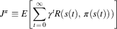
be the action set available to the agent. Each combination of starting state s i, action choice a i∈A and next state s j has an associated transition probability T(s i, a i, s j) and immediate reward R(s i, a i). The goal is to learn a policy π, which maps an action to each state so that the expected discounted reward J π is maximised:
 $$J^{\pi } \equiv E\left[ {\mathop{\sum}\limits_{t\,=\, 0}^\infty \gamma ^{t} R(s(t),\,\pi (s(t)))} \right]$$
where γ∈[0, 1) is the discount factor and expectations are taken over stochastic rewards and transitions. This goal can also be expressed using Q-values, which explicitly store the expected discounted reward for every state-action pair:
 $$Q(s,\,a) = R(s,\,a)\,{\plus}\,\gamma \mathop{\sum}\limits_{s'} T(s,\,a,\,s')\mathop {{\rm max}}\limits_{a'} \,Q(s',\,a')$$
In order to find the optimal policy, one can learn this Q-function and subsequently use greedy action selection over these values in every state. In RL, the agent typically does not have any knowledge about the underlying model, that is, the transition and reward function. Watkins described an algorithm, Q-learning, to iteratively approximate the optimal values Q*. In Q-learning (Watkins, Reference Watkins1989), a table consisting of state-action pairs is stored. Each entry contains the value for  $\hat{Q}(s,\,a)$
which is the learner’s current hypothesis about the actual value of Q(s, a). The
 $\hat{Q}$
-values are updated according to following update rule:
 $$\hat{Q}(s,\,a)\,\leftarrow\,\hat{Q}(s,\,a)\,{\plus}\,\alpha _{t} [R(s,\,a)\,{\plus}\,\gamma \mathop {{\rm max}}\limits_{a'} \,\hat{Q}(s',\,a')\,{\minus}\,\hat{Q}(s,\,a)]$$
where α t is the learning rate at time step t.
Provided all state-action pairs are visited infinitely often and a appropriate learning rate is chosen, the estimates  $\hat{Q}$
will converge to the optimal values Q* (Tsitsiklis, Reference Tsitsiklis1994).
2.1.1 Reward shaping in single-agent reinforcement learning
In many RL problems, the agent is only awarded a reward upon achieving a certain goal. For all other transitions R(s, a)=0. As can be seen from Equation (3), this reward is propagated through the state space. However, this process can be significantly time consuming.
One approach to overcome this problem, known as reward shaping, is the principle of giving additional numerical feedback to intermediate states that guide the learning agent. As manually determining which additional reward should be given can easily alter the agent’s intended goal (Randløv & Alstrøm, Reference Randløv and Alstrøm1998), Ng et al. introduced potential-based reward shaping (PBRS) (Ng et al., Reference Ng, Harada and Russell1999). In PBRS, the additional reward given to the agent is defined as the difference of a potential function Φ, defined over a source state s and a destination state s′:
 $$F(s,\,s') = \gamma \Phi (s')\,{\minus}\,\Phi (s)$$
where γ has the same value as in the Q-update rule which now takes following form:
 $$\hat{Q}(s,\,a)\,\leftarrow\,\hat{Q}(s,\,a)\,{\plus}\,\alpha _{t} [R(s,\,a)\,{\plus}\,F(s,\,s')\,{\plus}\,\gamma \mathop {{\rm max}\,}\limits_{a'} \hat{Q}(s',\,a')\,{\minus}\,\hat{Q}(s,\,a)]$$
Provided all additional reward are of this form, Ng and colleagues proved a single agent’s optimal policy would be unchanged (or more generally that the order of policies ranked by value would remain constant).
2.2 Multi-agent reinforcement learning
Problems in which multiple agents are acting simultaneously are commonly modelled as a Markov game (MG). In an MG, the state information s i∈S is the set of system states, which contains the information of all the agents. Actions are the joint result of multiple agents choosing an action individually. Let  $A_{k} \,{\equals}\,\{ a_{k}^{1} ,\:\,\ldots\,\:,\,a_{k}^{r} \} $
be the action set available to agent k, and k:1 … n, n being the total number of agents present in the system. Transition probabilities T(s i, a i, s j) in an MG depend on a starting state s i, ending state s j and a joint action from state s i, that is,
 $$a^{i} = (a_{1}^{i} ,\:\,\ldots\,\:,\,a_{n}^{i} )$$
with
 $a_{k}^{i} \in A_{k} $
. The reward function R k(s i, a i) is now individual to each agent k, meaning that agents can receive different rewards for the same state transition and joint action.
In a special case of the general MG framework, known as team games or multi-agent MDPs (MMDPs), all agents share the same reward function and the MG is purely cooperative. In this case, optimal policies still exist (Boutilier, Reference Boutilier1996; Claus & Boutilier, Reference Claus and Boutilier1998) and the optimal policy can be defined as the joint agent policy which maximises the payoff of all agents.
Alternatively, in the non-cooperative case one typically tries to learn an equilibrium between agent policies (Greenwald & Hall, Reference Greenwald and Hall2003; Hu & Wellman, Reference Hu and Wellman2003; Vrancx et al., Reference Vrancx, Verbeeck and Nowé2008). These systems require each agent to calculate or learn equilibria between possible joint actions in every joint state and as such assume that each agent retains estimates over all joint actions in all states. Moreover, these algorithms also face a selection problem if multiple equilibria exist.
2.2.1 Reward shaping in multi-agent reinforcement learning
From the description above it is clear that, learning in MAS adds several additional problems compared with learning in single-agent systems. One of the most important being the exponential increase in the state-action space in which the agents are learning. This significantly slows down the convergence of the learning and, as a consequence, their ability to adapt quickly to the changing environment too (Tumer & Khani, Reference Tumer and Khani2009).
Recently, Devlin and Kudenko introduced a method for transforming coordinated plans made together into a potential function to shape the rewards of the agents and guide their exploration in MAS (Devlin & Kudenko, In Reference Devlin and KudenkoPress). The authors illustrated that reward shaping in MAS also offers an elegant way to incorporate domain knowledge in the learning process and can speed up convergence. Moreover, it is also proven that PBRS in MAS does not change the Nash equilibria of the underlying stochastic game the agents are playing (Devlin & Kudenko, Reference Devlin and Kudenko2011).
In this paper, we use the approach of plan-based reward shaping (Grzes & Kudenko, Reference Grzes and Kudenko2008; Devlin & Kudenko, In Reference Devlin and KudenkoPress) to generate a potential function from a given individual greedy plan. The potential of the agent’s current state is given by
 $$\Phi (s) = CurrentStepInPlan\,{\times}\,w$$
where CurrentStepInPlan is the position of the current state of the agent in its plan and w a scaling factor defined as follows:
 $$w = MaxReward\,/\,NumStepsInPlan$$
As the scaling factor affects how likely the agent is to follow the heuristic knowledge, maintaining a constant maximum across all heuristics compared ensures a fair comparison. For environments with an unknown maximum reward the scaling factor w can be set experimentally or based on the designer’s confidence in the heuristic.
3 Sparse interactions
3.1 Concept
Recent research around MARL is trying to make a bridge between a complete independent view of the state of the system and a fully cooperative system where agents share and learn using all information. As mentioned before, learning using all this information slows the process. However, this information can still be used to determine when it should be used or when it is safe to ignore it. Terms such as local or sparse interactions were introduced to describe this new avenue in MARL. A new framework, called decentralised sparse interaction MDP (DEC-SIMDP) defines this new concept. Intuitively, his multi-agent framework consists of a set of single-agent MDPs for states in which agents are not interacting and a collection of MMDPs, containing the states and agents in which agents have to coordinate (Melo & Veloso, Reference Melo and Veloso2010). In order to define this DEC-SIMDP formally, we must first describe what is meant by the interaction between agents.
Definition 1 An agent k is independent of agent l in a state s∈S if the following conditions hold at state s:
∙ The transition probabilities for the local state of agent k at s do not depend on the state/action of agent l:
 $$\eqalignno{ P[s_{k} (t\,{\plus}\,1) = v_{k} \,\mid\,s(t) = u,\,a(t)=b] \cr\hskip-15pt= P[s_{k} (t\,{\plus}\,1) = v_{k} \,\mid\,s_{{{\minus}l}} (t) = u_{{{\minus}l}} ,\,a_{{{\minus}l}} (t) = b_{{{\minus}l}} ] $$
where the variables with subscript −l represent the system state information or joint actions, without the local information or action of agent l.
∙ It is possible to decompose the reward function, such that the reward signal both agents experience is independent of each others’ actions at state s.
So intuitively, this means that an agent k depends on the state information or the action of another agent l in a particular state s if either the transition function cannot be decoupled from the state information or action of agent l or the reward cannot be decomposed such that agent k does not experience any influence from the actions of agent l at s. An important remark concerning this definition must be made. First, these interactions are dependent on a particular agent in a particular state. This means that state s is not necessarily an interaction state for any other agent than agent k, although it certainly can be. Moreover, if there is a dependency between agent k and agent l at state s, it does not mean that there is also a dependency between agent l and agent k at state s. With other words, the relation is not necessarily symmetrical.
Given these rules for independence, sparse interactions are defined as follows.
Definition 2 In a DEC-MDP a set of agents K interact at state s if the following conditions simultaneously hold:
∙ If agent l∈K and ∃ agent k, such that agent k depends on agent l, then agent k∈K;
∙ If agent k∈K and agent k depends on agent l in state s, then agent l∈K;
∙ There is no strict subset K′ ⊂ K, such that the above conditions hold for K′.
If a set of agents K interact in state s, we refer to s Kas an interaction state for the agents in K.
Following from the definition of interaction states, we can now define interaction areas.
Definition 3 (Interaction area)An interaction area S Iis a set of joint states for which the following conditions hold:
1. S I⊂S Kfor some set of agents K, where S Kis the joint-state space of the agents in K;
2. ∃s ⇒ s∈S Iand s is an interaction state for the agents in K;
3. For any
 $s^{i} \in S^{I} ,\,a_{k}^{i} \in A_{k} $
and s j∉S I,
$P[S_{K} (t\,{\plus}\,1) = s^{j}\!\mid\!S_{K} (t) = s^{i} ,\,\vec {a}_{K} (t) = \vec {a}_{K}^{i} ] = \prod\limits_{k\in N} \,T(s_{k}^{i} ,\,a_{k} ,\,s_{k}^{j} )$
4. The set S Iis connected. This means that for every pair of states x, y∈S I, there exists a sequence of actions, such that y is reachable from x (or vice versa), through a set of states U ⊂ S I.


Which gives following definition for a DEC-SIMDP.
Definition 4 (DEC-SIMDP)An N-agent DEC-SIMDP with a set of L interaction areas  $\{ S_{1}^{I} ,\:\,\ldots\,\:,\,S_{L}^{I} \} $
is a tuple of
 $$\Gamma =\left( {M^{k} ,\,(M^{{I,l}} ,\,S^{{I,l}} )} \right),\:with\,k\in1,\:\,\ldots\,\:,\,L\,\;and\;l\in1,\:\,\ldots\,\:,\,L$$
where:
∙ Each M kis an MDP, M k=(S k, A k, T k, R k), that individually models agent k in the absence of other agents;
∙ Each (M I,l, S I,l) is an MMDP that represents a local interaction between K agents in the states of S I,l. For this joint state space representation holds:
$S_{K}^{I} \,\subset\,S\,\colon\,\,M^{{I,l}} = \left( {\left| K \right|,\,S_{K} ,\,A_{{1,\:}} _{{\,\ldots\,\:,\,{_\left| K _}\right|}} ,\,T,\,R^{I} } \right)$
, where R Irepresents the reward function for the agents in the interaction.

Melo and Veloso (Reference Melo and Veloso2009) introduced an algorithm, called learning of coordination (LoC), where agents learn in which states they need to condition their actions on other agents. As such, their approach is a way of solving a DEC-SIMDP. To achieve this they augment the action space of each agent with a pseudo-coordination action. This action will perform an active perception step. This could for instance be a broadcast to the agents to divulge their location or using a camera or sensors to detect the location of the other agents. This active perception step will decide whether coordination is necessary or if it is safe to ignore the other agents. As the penalty of miscoordination is bigger than the cost of using the active perception, the agents learn to take this action only in the interaction states of the underlying DEC-SIMDP. This approach solves the coordination problem by deferring it to the active perception mechanism.
De Hauwere et al. introduced CQ-learning for solving a DEC-SIMDP (de Hauwere et al., Reference De Hauwere, Vrancx and Nowé2010). This algorithm maintains statistics on the obtained immediate rewards and compares these against a baseline, which it received from training the agents independently of each other or by tracking the evolution of the rewards over time (de Hauwere et al., Reference De Hauwere, Vrancx and Nowé2011a). As such, states in which coordination should occur can be identified and the state information of these states is augmented to include the state information of the other agents. These are states in which there exists a statistical significant difference between the rewards of acting alone in the environment and acting with multiple agents or when the rewards radically change over time. Hence, this technique does not rely on external mechanisms, such as active perception as in LoC, to do so.
Kok et al. also introduced an approach where agents learn when it is beneficial to coordinate with other agents in fully cooperative games (Kok et al., Reference Kok, ’t Hoen, Bakker and Vlassis2005). They attempt to reduce the action space which agents need to consider, by letting the agents learn individually, and detecting differences in the reward signal based on different joint actions. Only in states where a dependency between the agents exists the agents will coordinate by selecting an action together in the joint action space, using a variable elimination algorithm.
3.2 Future Coordinating Q-learning
All of these approaches however assume that states in which coordination is required can be identified solely based on the immediate rewards. This assumption might not always be met and thus there is need for more general algorithms capable of dealing with this issue, as all currently existing techniques fail in such settings. In this paper, we focus on enhancing, by applying reward shaping, the learning process of a technique that can handle delayed coordination problems using sparse interactions. This technique, called FCQ-learning, is capable of detecting the influence from other agents several time steps ahead.
In this section, we explain this approach of dealing with delayed coordination problems. As explained, the view of the algorithms described in the previous section is too limited, as it is not acceptable to assume that the need for coordination is reflected immediately in the reward signal following the action. Learning using the full MG view of the system, such delayed reinforcement signals are propagated through the joint-state space and algorithms using this MG view can still learn optimal policies. It should however be clear by now that this view of the system is not a realistic one as it slows learning. A DEC-SIMDP is more realistic as it models exactly the coordination dependencies that exist between agents in a limited set of states and allows to learn without always selecting actions based on the full MG view. As it is not modelled how these dependencies can be resolved, the DEC-SIMDP is still applicable as a framework for delayed coordination problems. Note that there is a clear distinction between being able to observe the other agents and learn when to use this information, versus always learning using this information as illustrated in Melo and Veloso (Reference Melo and Veloso2009) and de Hauwere et al. (Reference De Hauwere, Vrancx and Nowé2010).
The idea of FCQ-learning is that agents learn in which of their local states they will augment their state information to incorporate the information of other agents and use a more global system state based on statistical tests on the reward signal. As such, agents only learn using their local states and a limited number of augmented states in which statistical tests have indicated that observation is beneficial.
This idea is represented in Figure 1. The local states for one agent are represented at the bottom. In its local states labelled 4 and 6 the agent decided to augment its information to include the state information of another agent illustrated at the top. It has augmented local state 4, with local states 1, 2 and 3 of another agent and local state 6 with local states 1 and 2 of another agent. Note that an agent’s local state only contains state information about the agent itself such as its own location, battery level, other sensory input, etc. Whereas, the global state contains the local state information about all agents. In this example, the agent is learning using a state space consisting of 14 states, whereas traditional algorithms would learn using a state space of 81Footnote 1. Also note that this augmentation of states is not symmetrical. One agent could detect the need for coordination before another agent and already solve it, before this other agent detected this need.
The state information of states 4 and 6 is augmented to incorporate additional information of another agent in order to solve coordination problems. State 4 is augmented with states 1, 2 and 3 and state 6 with states 1 and 2 of another agent

The major challenge is detecting in which states the state information must be augmented. During learning, FCQ-learning samples the returns the agent collects in each local state, and groups them according to the local state of other agents. This principle is shown in Figure 2. Using these samples, the agent then performs a Friedman statistical test which can identify the significance of the difference between the different local states of the other agents for its own local state. This test indicates whether the returns are drawn from the same distribution or are coming from different distributions. In Figure 2, Agent 1 starts sampling the rewards until termination of the episode in local state x i based on the local state information y i, y j and y k of Agent 2. Note that it is only observing this information to collect samples, it is still learning using only its own local state information. If enough samples have been collected and if a significant difference is detected among these states, the state information for the local state of Agent 1 is augmented to include the information of the other agent for which the difference was detected (as illustrated in Figure 1) and the agent will select actions based on the augmented state information. In de Hauwere et al. (Reference De Hauwere, Vrancx and Nowé2011c), the authors also describe how the number of samples can be reduced in case a baseline where agents are not being influenced is available.
Agent 1 in local state x i is collecting rewards until termination of the episode based on the local state information of Agent 2
At every time step, when the agent selects an action, it will check if its current local state is a state which has been augmented and contains the state information of other agents. If so, it will condition its action based on this augmented state information, otherwise it can act independently using only its own local state information.
Two situations for updating the Q-values are distinguished:
1. An agent is in an augmented state: following update rule is used:
(8)where Q k stands for the Q-table containing the local states, and
$$Q_{k}^{{{\rm aug}}} (js,\,a_{k} )\,\leftarrow\,(1\,{\minus}\,\alpha _{t} )Q_{k}^{{{\rm aug}}} (js,\,a_{k} )\,{\plus}\,\alpha _{t} [r(js,\,a_{k} )\,{\plus}\,\gamma {\rm max}_{{a'_{k} }} Q_{k} (s',\,a'_{k} )]$$
$Q_{k}^{{{\rm aug}}} $
contains the augmented states (js). Note that this augmented Q-table is initially empty as we use a bottom-up approach to learning sparse interactions. The Q-values of the local states of an agent are used to bootstrap the Q-values of the states that were augmented with global state information. This is to capture the idea of a sparse interaction, where agents only influence each other in certain states, after which they can act independently again.2. An agent is in a local state: the Q-learning rule of Equation (3) is used with only local state information.


The case where the Q-table with joint states to bootstrap is not considered in this update scheme since at time step t an agent cannot know that it will be in a state where coordination will be necessary at time step t+1 as this will also depend on the actions of other agents.
For every augmented state a confidence value is maintained which indicates how certain the algorithm is that this is indeed a state in which coordination might be beneficial. If the augmented state of a local state is visited, the confidence value is increased. Otherwise the confidence values of all the augmented states that have been created from the current local state are decreased. This ensures that states where an agent would request state information about another agent, but where this state information does not correspond to the augmented state, are reduced again to states where agents only consider local state information. By reducing this value less than it is increased, some fault tolerance is added against too quickly reducing states to local states again.
The algorithm is more formally described in Algorithm 1.
4 Context-sensitive reward shaping
An agent, learning in an environment, can have different subgoals it is trying to achieve while accomplishing the global goal of the task at hand. Incorporating all these subgoals into one shaping function is not feasible. The idea we present here is to have different appropriate shaping functions, that depend on the context the agent is currently in. This context is defined by the subgoal it is currently trying to accomplish. The shaping function for a context will guide the agent towards achieving the particular goal of that context. These shaping functions can be defined for a single agent, or can be generated from a joint plan including the other agents’ state. As acknowledged by Devlin and Kudenko (In Reference Devlin and KudenkoPress), individual plans might contain conflicting knowledge, which results in agents interfering with each other. On the other hand, shaping functions based on joint plans require prior coordination and knowledge of interaction states. As this may not always be possible, we propose to use a different shaping function when acting individually or when coordinating. If these contexts can be detected automatically, agents can autonomously switch to a different shaping function for the particular context the agent is currently in. This allows the designer of the system to have multiple simple shaping functions, rather than try to build one shaping function that covers all the subtleties that occur when multiple agents act in the same environment.
We implement our approach to context-sensitive reward shaping by using FCQ-learning to detect the different contexts. FCQ-learning samples the state space and will automatically augment certain states to include state information about other agents if the agent is influenced by them. This means that an agent can be in one of following contexts:
1. Individual: the agent is not influenced by any other agent and only uses local state information to select its actions.
2. Coordinating: the agent is influenced by another agent and uses augmented state information to select actions.
As explained above, a different shaping function is to be used in these different contexts as they have different subgoals. In the individual context the agent is trying to accomplish its goal and collect a reward upon achieving it. It is not influenced by any other agent in the states that are part of this context and hence it selects its actions independently. In the coordinating context, the agent is in an interaction area, its transitions and rewards are dependent on the state information and actions of other agents and its goal in this context is to select the best action that solves the coordination problem. This is not necessarily the same action it would select to reach its individual goal. As an example to clarify this, we explain the set-up of the experiments we used. These are navigation tasks, where both agents have to reach the same location but the order in which they reach this location will determine the reward they receive. Agent 1 needs to enter the goal location before Agent 2. The global goal of the system is for both agents to reach the goal location in the correct order. Agents are initially unaware of the fact that they have to coordinate with this other agent in order to avoid collisions and they also do not have any information about the order in which they need to reach the goal. This is learned through the statistical tests that FCQ-learning performs on the reward signal and as such, agents learn different policies for those situations where they are independent of other agents and for those where there is a dependency between them.
In the Individual context the shaping function used is calculated as described in Section 2.2. The potential is calculated from a high-level plan which contains landmarks from the initial position to the goal. So the potential is actually a gradient that steers the agent in the general direction of the goal, as if it was a beacon. As the potential difference from Equation (4) is increased as they reach landmarks that are located nearer to the goal, agents receive a positive intermediate feedback, while they are learning a low-level navigation policy. In this context, agents ignore each other and are only concerned with reaching the goal.
In the Coordinating context the global goal of the system is used to shape the rewards. Agent 1, which has to reach the goal first, keeps the same potential function and is, therefore, still guided towards the goal. Agent 2 receives an incentive to not reduce the distance between itself and Agent 1. As such we are certain that Agent 1 can reach the goal first and accomplish the global goal of the system. This shaping function represents domain knowledge about the fact that agents have to reach the goal in a certain order and as such gives the agent immediate feedback about the coordination, rather than having to wait several episodes until the final reward that is given upon completion of the episode is propagated to the coordination states.
The idea is presented visually in Figure 3. Both shaping functions follow the assumptions of Devlin and Kudenko (Reference Devlin and Kudenko2011) and as such the original equilibria of the game are not altered.
Context-sensitive use of reward shaping in multi-agent systems
5 Experimental evaluation of context-sensitive shaping functions
5.1 Gridworld experiments
To validate this approach to reward shaping within the FCQ-learning framework, we first use two discrete, gridworld navigation with priority tasks; Grid game 2 and TunnelToGoal as shown in Figure 4.
Navigation games: (a) Grid game 2 and (b) TunnelToGoal
The initial positions are marked with Si for each agent i. The goal position is indicated with the letter G. Each cell can only be occupied by one agent at any given time. These environments induce some form of coordination problem, where following the shortest path to the respective goals of the agents would result in collisions. Moreover, agents need to coordinate during the episode in order to enter the goal in the correct order and achieve the highest reward. All experiments were run for 10 000 learning episodes (an episode is completed if all agents reach their respective goal state) and averaged over 20 independent runs. The experiments were run using a learning rate of 0.2 and a discount factor γ=0.95. Exploration was regulated using a fixed ε-greedy policy with ε=0.1. Reaching the goal results in a reward of 20 in Grid game 2 and of 600 in TunnelToGoal if the agents reach the goal in the correct order (i.e. Agent 1 before Agent 2). Otherwise, the maximum reward they can achieve is 10 in Grid game 2 and 300 in TunnelToGoal.
If the agents collide they remain in the location they were in before the collision and receive a penalty of −10 for colliding. All transitions are assumed to be stochastic, they succeed in 90% of the cases or, in the other 10% agents are moved to one of the adjacent cells at random.
Two shaping approaches were used to evaluate the benefits of context-sensitive reward shaping and compared with FCQ-learning without shaping, denoted as No shaping. The first one was to only use the individual shaping function. So agents were only guided towards the goal using a shaping function derived from a high-level plan. These results are denoted as Simple shaping. We also tried to solve these problems using only the coordination shaping function. In this function, agents are given an incentive to approach the goal in the correct order, but are not given any additional information about how to reach the goal. This however resulted in the fact that agents never managed to reach the goal as these functions gave the agents an incentive to solve a problem that was not apparent yet. Agents were still learning a policy to reach the goal, but were penalised by the shaping functions if they approached the goal in the wrong order. In the initial stages of the learning process the reward of reaching the goal is not yet propagated through the state space, so Agent 2 received penalties in many states that the agent has to explore in order to find the goal. Due to this bad shaping function, Agent 2 learned a policy where it tried to move as far away as possible from the other agent (as this resulted in a small positive-shaped reward). Finally, the results for context-sensitive shaping functions are denoted as Context shaping.
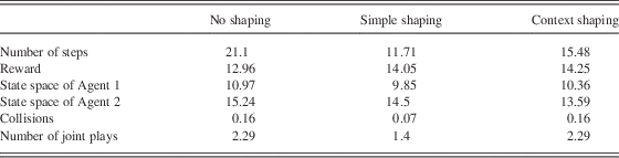
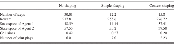
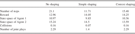
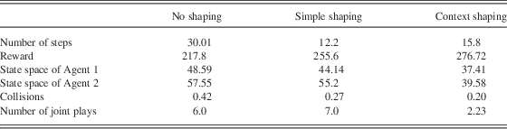
We will begin by describing the qualitative results of the learned policies for FCQ-learning without shaping, with a simple shaping function and with a context-sensitive shaping function. We compare the number of steps the agents need to complete an episode, how often they collide during an episode, the average reward they received per episode, the size of the state space in which they are learning and how often they use the augmented state space (= #joint plays). These results were obtained by taking the average over the last 100 episodes (while still using the ε-greedy action selection mechanism).
Even in the Grid game 2 environment, which is relatively small, the benefit from applying context-sensitive reward shaping can clearly be seen. The number of steps to finish an episode is reduced with nearly 30% and the reward is increased with 10% compared with not using any shaping function. The simple shaping function manages to reach the goal faster as it exclusively uses a shaping function that encourages this.
In the TunnelToGoal environment we see even bigger changes. The number of steps required for both agents to complete an episode is almost halved with context-sensitive shaping and is even lower for the simple shaping function.
Also in this environment, surprisingly, in many cases the slowest agent turned out to be Agent 1 if no shaping was used. This effect occurred also if only a simple shaping function was used, albeit less often. This shaping function is indeed the correct shaping function for Agent 1. As this agent had to reach the goal first in order to reach the highest reward, without shaping the agents do not manage to reach the same performance level as the agents with simple or context-sensitive reward shaping. FCQ-learning alone has a larger state space and uses augmented state information more often per episode than with reward shaping. This is due to the fact that the incorporation of background knowledge in the shaping function when using augmented state information significantly helps the agent reach the optimal solution (in which Agent 1 has to reach the goal first).
In both environments the state space of Agent 2 contains more augmented states. This can be explained by the fact that this agent has to verify where Agent 1 is currently located in order to (possibly) make a detour, allowing Agent 1 to reach the goal first.
In Figure 5, we show the number of steps needed to complete an episode during the learning process. On the left we see the results for the Grid game 2 environment, on the right the results for the TunnelToGoal environment. In the larger TunnelToGoal environment we clearly see the effect of reward shaping. Agents are learning a lot faster to reach their goal. We also see that context-sensitive shaping learns a stable policy more quickly than simple shaping as it has a specific shaping function that is used to solve the detected conflicts that occur between the agents.
Average number of steps to complete an episode for Grid game 2 (left) and TunnelToGoal (right)
The consequence of this increase in learning speed is also reflected in Figure 6. This figure shows the average number of collisions per episode. In the beginning of the learning process, while the agents are still identifying joint states, we see a higher number of collisions in the agents with reward shaping. As the shaping helps them reach their goal faster, the number of collisions is also increased sooner. Note that these collisions are necessary for FCQ-learning to identify the states in which they should use augmented state information. If agents only use a single shaping function, this function leads them to states in which agents influence each other, which results in lower rewards as these shaping functions do not take other agents into consideration and hence the agents could learn the wrong coordination policy. FCQ-learning with context-sensitive shaping on the other hand switches to a different shaping function in these states in order to solve the coordination problem that occurs in these states. This happens around learning episode 1000, after which we see a sudden drop in the number of collisions per episode. In Grid game 2 we see the same effect, albeit a lot more subtle as this environment is a lot smaller than TunnelToGoal.
Average number of collisions per episode for Grid game 2 (left) and TunnelToGoal (right)
The rewards obtained by the agents per episode, shown in Figure 7, also follow the same pattern and around episode 1000 we see an increase in the obtained rewards, due to this decrease in the number of collisions. If no shaping function is used, it takes FCQ-learning a lot longer to reach a stable policy (which also performs worse) as when a shaping function is used. The agents using context-sensitive shaping also reach a higher reward than the agents using a single shaping function.
Average reward per episode for Grid game 2 (left) and TunnelToGoal (right)
Finally, we show the number of times agents used augmented state information per episode in Figure 8. FCQ-learning without a shaping function has a larger state space (which can also be seen in Tables 1 and 2). This occurs because agents do not get feedback on their interaction immediately. Instead, the effect of having coordinated correctly is only reflected in the goal state several time steps ahead and, therefore, it takes several learning episodes for this feedback to be back propagated. Meanwhile, other states are being augmented unnecessarily. This also explains why FCQ-learning without shaping does not find the correct coordination policy as often as with context-sensitive reward shaping. The agent could have learned contradicting policies in the different augmented states, as there is no feedback between augmented states (they are bootstrapped with local state information). Learning to coordinate between different augmented states will take many learning episodes, especially since interactions are sparse and becomes more difficult each time new augmented states are identified. The agents using a single shaping function need the augmented state information more often because even in these augmented states the agent receive an incentive to reach the goal as quickly as possible, without considering the other agents. As such, more states are identified as agents receive higher-shaped rewards for miscoordination. The number of joint plays for context-sensitive reward shaping decreases over time as agents converge to a policy more quickly and the number of augmented states that are visited decreases over time. Moreover, this also results in a decrease in the size of the state space because, as explained in Section 3.2, the confidence level of augmented states that are not visited often enough is decreased after which eventually they are being reduced to local states again.
Average number of joint plays per episode for Grid game 2 (left) and TunnelToGoal (right)
Final results for the Grid game 2 environment
Final results for the TunnelToGoal environment
5.2 Air traffic control
Recently, institutions like the Federal Aviation Authority (FAA) and EUROCONTROL started using computational tools during the development of new air traffic control (ATC) procedures that allow them to model and simulate a new procedure and have immediate feedback in terms of the impact on controller workload, overall delays and distances or fuel burned by the aircraft, etc. One such tool is the fast-time simulator. An important characteristic of this tool is that it offers a low cost solution to have a fast and reliable feedback to validate new ATC procedures. Moreover, the accuracy of these tools has increased a lot in recent years and are more and more used by airport staff to simulate new procedures and operations. The term ‘fast time’ is derived from the fact that the simulation clock runs faster than a regular clock. The simulation speed is only limited by the performance of the computer on which it is running. The availability of such tools allows the use of algorithms such as FCQ-learning in ATC. FCQ-learning can be used within such a fast-time simulator as a decision support tool for the controller and different solutions can be presented to the controller, which can each be optimised based on different criteria. Moreover, the use of context-sensitive reward shaping assists the algorithm in finding solutions based on individual controller preferences as well. In this section, we further evaluate the combination of FCQ-learning with context-sensitive shaping functions in a simulation of ATC in which the focus lies strongly on correct coordination among the agents.
In this simulation the air space is divided into sectors representative of vast three-dimensional (3D) areas in which planes are allowed to fly over predefined waypoints. For every sector, there is a controller responsible for managing the aircraft within that sector. This means they should detect potential conflicts during the flight and solve them. Preferably, this is done before handing over control of an airplane to the next sector, so small short-term changes of the trajectory are preferred. Several options exist for solving this kind of conflict. Controllers can issue orders to one or both aircraft, such that aircraft can alter its speed, its altitude, its heading, etc. in order to avoid the conflict. Depending on the aircraft type different solutions are preferred in terms of fuel consumption, comfort for the passengers, etc.
Controllers currently select their solutions based on their past experience and what they believe to be good solutions. This experience is an ideal source for designing shaping functions for the interactions that occur between agents.
Often, the conflicts are identified too late and controllers cannot resolve the conflict within their own sector. In these situations the controller has to hand over the control of the plane and its repair plan to the next sector. We performed a fast-time simulation of this kind of problem using three aircraft in a sector and used FCQ-learning to learn a solution. Each agent represents one aircraft, learning a trajectory through the sector and how to solve the conflict. After learning, the solution of the entire MAS can be communicated to the controller as a suggestion on how to solve the conflict.
The 3D problem of one sector is displayed in Figure 9. If the aircraft would follow their original flight path (indicated by the dashed lines) a conflict would occur in the near future. As can be seen, the different planes have different exit points out of the sector and they want to follow their plan as closely as possible. The possible actions that are allowed are limited because aircraft always have to fly over waypoints (indicated by the flags on the ground). As a result, this limits the number of decision points in which potential conflicts can be solved. Moreover, the conflict is preferably solved within this sector. Hence the problem has to be solved in a timely fashion. Suppose A prefers to continue its descent, whereas for B it is of lesser importance if it would have to stop climbing for some time in order to solve the conflict. C however needs to reach its cruising altitude as soon a possible to avoid noise pollution on the ground. As mentioned, the controller can only solve this problem respecting the constraints of flying from one waypoint to the other.
Three-dimensional illustration of coordination problems in air traffic control
An abstract representation of the problem is shown schematically in Figure 10. This original plan (which is indicated by the bold line for the different aircraft) would result in a conflict after six time steps. Each agent/aircraft has various alternatives to their original plan. The alternatives all have different deviations from the original flight plan and different alternatives are optimal for different aircraft. The nodes in the graph in which agents can select multiple actions are waypoints. All nodes are identified by an ID number and represent the local state information of agents. The actions the aircraft can take (descend, ascend, speed up, continue, hold) are represented by the numbers on the edges. Note that agents cannot select all actions in all nodes, and that in some nodes, they have to carry out the same action multiple times (i.e. descend followed by ascend makes no sense). This also captures the concept of time as slowing down means it will take them longer to reach a certain waypoint (i.e. more nodes in the graph). The different alternative solutions for the aircraft are also overlapping in certain regions of the space, causing multiple coordination problems. In the figure the grey nodes indicate the starting positions of the agents. Agent 1 in state 1, Agent 2 in state 27 and Agent 3 in state 42. All agents have different alternative solutions to overcome the problem and continue their original flight plan. The problem is overcome when the agents reach node 26. The optimal solution (in terms of fuel consumption, comfort, etc.) is for Agent 1, to reach this state the fastest, followed by Agent 2 and finally Agent 3. The shaping function for the individual navigation task was derived from the original flight plan in which the aircraft have to fly over particular waypoints. The shaping function for the coordination task was calculated based on the optimal policy in which agents receive an incentive to align themselves in the correct order to reach node 26. If agents selected an action which caused a wrong alignment, they were penalised. For instance, Agent 2 was penalised if it increased its speed if it was already closer to the goal than Agent 1.
Schematic representation of the state-action space of one sector in the air traffic control problem. Nodes, identified by an ID, represent the waypoints, the numbers on the edges represent the actions the aircraft can take
The results for this domain without shaping and with context-sensitive shaping are shown in Figure 11. The results are again averaged over 50 independent runs and parameter settings were the same as for the gridworld experiments.
Average reward per episode for the air traffic control domain (left) and sample results of one run (right)
On the left-hand side we show the average reward the agents collect over time and observe similar results as with the gridworld experiments, that is that reward shaping helps the agent to reach the coordination policy a lot faster than without reward shaping.
The figure on the right-hand side shows the results of the number of steps per agent during learning in a sample run. Note that Agent 1 has to reach the goal, before Agent 2, which, in its turn, has to reach the goal before Agent 3. These coordination rules can be extracted from human controllers and reward shaping allows us to express them in a natural way. As these shaped rewards are incorporated into the immediate reward signal, the agents learn the correct coordination policy very quickly. The optimal policy if agents are acting independently requires six time steps to reach the goal. As can be seen, Agent 1 has learnt this policy and Agent 2 only needs one extra time step, whereas Agent 3 needs an additional two to reach the goal. All this is learnt without any communication about the agents’ intentions and only a limited number of additional states in which other agents are being observed. Per episode, agents only observe the other agents two times on average, whereas FCQ-learning without shaping functions observes the state information of other agents six times per episode. Note that these numbers are the sum of all agents, not the number of times each agent uses augmented state information. Therefore, to conclude, the agents achieve a better level of performance with less information about other agents, thanks to the inclusion of reward shaping.
6 Conclusion
When trying to learn good policies in environments where multiple agents are present, many things must be taken into consideration when selecting an algorithm. For instance, is all the information about the other agents available or can they obtain it through communication, do the agents have common interests, how many other agents are present, etc. If all information is available learning in the entire joint-state joint-action space will be beneficial, but at a high cost of a long learning time. If this cost is too high, independent learners could be used, but the outcome of this approach is very uncertain. For these reasons a new research track in multi-agent learning research received increasing interest lately. Using sparse interactions and taking other agents into consideration when this is necessary or beneficial seems to be improving both the final outcome of the learning process as well as the speed to reach this outcome.
FCQ-learning is an algorithm that aims at learning a policy in an environment where multiple agents are loosely coupled. This means that agents influence each other only in certain regions of the state space. Moreover, we assume that agents are able to complete a goal independently, but coordinating is beneficial in the sense that it results in a higher payoff some time in the future. FCQ-learning is capable of detecting such delayed coordination problems. In states in which such problems are detected, the state space is augmented to include the state information of other agents and select actions independently using this augmented state information. This paper presents an extension to FCQ-learning through the incorporation of reward shaping and an extension to PBRS to become context sensitive.
Reward shaping has already proved in both single and MAS to be able to significantly speed up the learning process by giving intermediate rewards, based on some domain knowledge.
We have demonstrated empirically how, in MAS, different shaping functions can be used, depending on the context of the agent, that is, is it interacting with another agent or is it not. This distinction allows us to benefit from both the speed up achieved by FCQ-learning and the speed up obtained through reward shaping. We evaluated our approach using a navigation task and an ATC simulation, with both feature a delayed coordination problem, and observed a significant speed up in the convergence to a stable policy, as well as an improvement in the final policy learned by the agents compared with not using any shaping function or only a single shaping function. We also observed that if a bad shaping function was used this resulted in extremely bad performance for the agents.
These results motivate future research into whether more complex contexts of agents can be automatically detected and if a mapping from context to shaping function can be learned autonomously by the agents.
Acknowledgements
The authors would like to thank the anonymous reviewers as well as the editors of the journal for their constructive comments.