1 Introduction
There is today a general acceptance that high-Reynolds-number jet turbulence has large-scale organized flow structures that are intrinsically related to jet noise, especially in the case of circular jets and their low-frequency aft-angle noise radiation (Jordan & Colonius Reference Jordan and Colonius2013; Cavalieri, Jordan & Lesshafft Reference Cavalieri, Jordan and Lesshafft2019). A number of studies support the view that solutions from linear stability theory, with the turbulent mean field used as a base flow, can capture the essential aspects of such coherent structures underpinning sound radiation (Michalke Reference Michalke1970; Crighton & Gaster Reference Crighton and Gaster1976; Michalke Reference Michalke1984; Tam & Burton Reference Tam and Burton1984; Suzuki & Colonius Reference Suzuki and Colonius2006; Gudmundsson & Colonius Reference Gudmundsson and Colonius2011; Cavalieri et al. Reference Cavalieri, Rodríguez, Jordan, Colonius and Gervais2013; Jordan & Colonius Reference Jordan and Colonius2013; Sinha et al. Reference Sinha, Rodríguez, Brès and Colonius2014). It is therefore important to investigate the linear stability of non-circular jets, particularly for nozzle shapes and passively or actively controlled configurations associated with noise reduction (Zaman, Bridges & Huff Reference Zaman, Bridges and Huff2011).
Early work on the stability of an elliptic vortex sheet can be traced back to Crighton (Reference Crighton1973). Morris (Reference Morris1988) later extended the analysis to finite-thickness shear layers, with an analytic base-flow representation that allowed solutions to become separable in elliptical coordinates. For most non-circular jets, however, the stability equations are not separable, and further work was carried out on the development of more general methods to account for arbitrary cross-sections (Koshigoe & Tubis Reference Koshigoe and Tubis1986, Reference Koshigoe and Tubis1987; Koshigoe et al. Reference Koshigoe, Gutmark, Schadow and Tubis1988; Tam & Thies Reference Tam and Thies1993; Baty & Morris Reference Baty and Morris1995). The attention was, nonetheless, mostly restricted to elliptic, triangular and rectangular jets.
The interest in corrugated mean flows appears more recently. Kawahara et al. (Reference Kawahara, Jiménez, Uhlmann and Pinelli2003) investigated the temporal stability of a corrugated plane vortex sheet, with a particular choice of conformal mapping, as a model for the instability of streaks in turbulent boundary layers. Corrugations were found to be always stabilizing in the case of free sheets, for both varicose and sinuous modes. The wall influence was also addressed, given their main focus in boundary layers. The obtained solutions were related to oblique Kelvin–Helmholtz waves, with eigenfunctions following local intensifications of streamwise vorticity, aligned with geometric features of the sheet. A spatial stability analysis, which is more in line with the jet problem, was carried out by Ostrikov, Kopiev & Kasyanov (Reference Ostrikov, Kopiev and Kasyanov1998) with a sinusoidal form of corrugation. The model was later extended to cylindrical coordinates by Kopiev et al. (Reference Kopiev, Ostrikov, Chernyshev and Elliott2004), and further investigated under subsonic conditions (Kopiev & Ostrikov Reference Kopiev and Ostrikov2012). From these studies it was revealed that even small corrugation amplitudes, apart from promoting a mixture of azimuthal wavenumbers in the solution, were able to couple
 $m=0$
with
 $m=\pm N$
(the other wavenumbers that are multiples of the
 $N$
number of periodic corrugations) at
 $St<0.1$
. This occurred only for
 $N\geqslant 3$
. Since the most azimuthally coherent turbulent structures are also the most efficient in driving the near-field pressure at lower frequencies (Tinney & Jordan Reference Tinney and Jordan2008; Cavalieri et al.
Reference Cavalieri, Rodríguez, Jordan, Colonius and Gervais2013), it was suggested that this mechanism could be significant for jet aeroacoustics.
More realistic situations were addressed by Gudmundsson & Colonius (Reference Gudmundsson and Colonius2007), with stability calculations performed using mean flows acquired by Bridges & Brown (Reference Bridges and Brown2004), consisting of velocity measurements in Mach
 $0.9$
jets issuing from circular and serrated nozzles; such nozzle serrations are called chevrons. Their results were summarized by Sinha et al. (Reference Sinha, Gudmundsson, Xia and Colonius2016a
). Most recent developments are now more concerned with solutions that account for the mildly non-parallel base flow by using a reformulation of the parabolized stability equations (PSE) for non-axisymmetric configurations (Uzun et al.
Reference Uzun, Alvi, Colonius and Hussaini2015; Sinha, Rajagopalan & Singla Reference Sinha, Rajagopalan and Singla2016b
). The closeness of the stability results from the inviscid (Uzun et al.
Reference Uzun, Alvi, Colonius and Hussaini2015) and the viscous formulation (Sinha et al.
Reference Sinha, Gudmundsson, Xia and Colonius2016a
) also reflects the minor role that viscosity plays in the problem. The fair agreement between these solutions with results from experiments and large eddy simulations supports the applicability of linear stability theory to describe the behaviour of coherent turbulent structures that exist in corrugated jets.
In the present study, our aim is to investigate the effect of base-flow changes on the spatial stability of corrugated jets. The attention will be restricted to a locally parallel framework, as we aim to explain some puzzling features that were observed in our simultaneous prior studies (Lajus, Cavalieri & Deschamps Reference Lajus, Cavalieri and Deschamps2015; Sinha & Colonius Reference Sinha and Colonius2015). In particular, somewhat different trends were found in the two independent locally parallel investigations of the same jet. These are hereby explained as arising from the two distinct approaches pursued for modifying the base flow, and to the focus on different axial stations (
 $x/D=0.5$
and
 $x/D=2.0$
) of the jet. Here we propose a more systematic approach to explore the effect of corrugations on jet stability, with the introduction of a parametrized base flow that allows us to track solutions as a jet is incrementally deformed from a circular to a corrugated shape. The stability results are also expected to help in the development of better noise suppression devices, highlighting the most relevant features of the base flow.
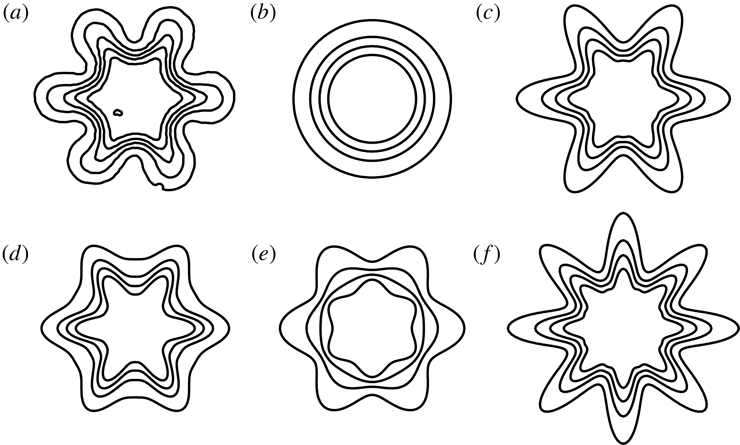
The paper is organized as follows. First, in § 2, the linear stability equations and the numerical solution scheme are presented. The mean-flow parametrization is discussed in § 3. In § 4, the origin of multiple unstable solutions is explained by tracking eigenvalues as the parametrized base flow is gradually varied from circular to corrugated. In § 5, we report growth rates and phase speeds for base-flow deformations related to usual design parameters of corrugated nozzles, namely penetration and number of corrugations. The influence of penetration is also investigated separately, by varying only the shear-layer position and shear-layer thickness. A sample of such base-flow deformations is shown in figure 1. In § 6 we discuss the limitations of our theoretical exploration and how we expect that the obtained results could be relevant to the radiated noise of corrugated jets. The main conclusions are presented in § 7.
Sample of investigated base-flow deformations corresponding to: (a) the original mean flow (Bridges & Brown Reference Bridges and Brown2004), (b) zeroth-order approximation, (c) increased penetration, (d) perturbation only applied to the shear-layer position, (e) perturbation only applied to shear-layer thickness and (f) increased number of periodic lobes.

2 Linear stability equations
2.1 Mathematical formulation
The usual approach of stability analysis involves the linearized version of non-dimensional Euler or Navier–Stokes equations, under some simplifying assumptions regarding the base flow (Sipp & Lebedev Reference Sipp and Lebedev2007; Taira et al.
Reference Taira, Brunton, Dawson, Rowley, Colonius, McKeon, Schmidt, Gordeyev, Theofilis and Ukeiley2017). Such a linearized and non-dimensional (by the jet diameter
 $D$
, ambient sound speed
 $a_{\infty }$
and density
 $\unicode[STIX]{x1D70C}_{\infty }$
) set of Euler equations for the disturbances
 $\boldsymbol{q}(\boldsymbol{x},t)=[u_{x},u_{r},u_{\unicode[STIX]{x1D703}},\unicode[STIX]{x1D70C},p]^{\text{T}}$
, in cylindrical coordinates (
 $\boldsymbol{x}\equiv (x,r,\unicode[STIX]{x1D703})$
), can be written schematically as
 $$\begin{eqnarray}\displaystyle {\mathcal{L}}_{\bar{\boldsymbol{q}}}\{\boldsymbol{q}(\boldsymbol{x},t)\}=0. & & \displaystyle\end{eqnarray}$$
Here
 ${\mathcal{L}}_{\bar{\boldsymbol{q}}}\{\cdot \}$
is the linearized operator, which has the form
 $$\begin{eqnarray}\displaystyle {\mathcal{L}}_{\bar{\boldsymbol{q}}}\{\cdot \}=\frac{\unicode[STIX]{x2202}\{\cdot \}}{\unicode[STIX]{x2202}t}+\boldsymbol{A}(\bar{\boldsymbol{q}})\frac{\unicode[STIX]{x2202}\{\cdot \}}{\unicode[STIX]{x2202}r}+\boldsymbol{B}(\bar{\boldsymbol{q}})\frac{\unicode[STIX]{x2202}\{\cdot \}}{\unicode[STIX]{x2202}x}+\boldsymbol{C}(\bar{\boldsymbol{q}})\frac{\unicode[STIX]{x2202}\{\cdot \}}{\unicode[STIX]{x2202}\unicode[STIX]{x1D703}}+\boldsymbol{D}(\bar{\boldsymbol{q}})\{\cdot \}. & & \displaystyle\end{eqnarray}$$
The coefficients
 $\boldsymbol{A}$
through
 $\boldsymbol{D}$
are only dependent on the mean flow
 $\bar{\boldsymbol{q}}(\boldsymbol{x})$
,
 $$\begin{eqnarray}\displaystyle \bar{\boldsymbol{q}}(\boldsymbol{x})=[\bar{u}_{x}(r,\unicode[STIX]{x1D703}),\bar{u}_{r}(r,\unicode[STIX]{x1D703}),\bar{u}_{\unicode[STIX]{x1D703}}(r,\unicode[STIX]{x1D703}),\bar{\unicode[STIX]{x1D70C}}(r,\unicode[STIX]{x1D703}),\bar{p}(r,\unicode[STIX]{x1D703})]^{\text{T}}, & & \displaystyle\end{eqnarray}$$
which in turn does not depend on time or axial coordinate (with the parallel-flow assumption). It follows that the solutions for
 $\boldsymbol{q}(\boldsymbol{x},t)$
become separable in these directions using normal modes
 $$\begin{eqnarray}\displaystyle \boldsymbol{q}(\boldsymbol{x},t)=\widetilde{\boldsymbol{q}}(r,\unicode[STIX]{x1D703})\text{e}^{\text{i}\unicode[STIX]{x1D6FC}x}\text{e}^{-\text{i}\unicode[STIX]{x1D714}t}, & & \displaystyle\end{eqnarray}$$
where
 $\unicode[STIX]{x1D6FC}$
and
 $\unicode[STIX]{x1D714}$
are the axial wavenumber and circular frequency, respectively. In the case of spatial stability formulation, the interest lies in finding (possibly complex) solutions for
 $\unicode[STIX]{x1D6FC}$
for a given real-valued
 $\unicode[STIX]{x1D714}$
. When considering strictly parallel (
 $\bar{u}_{r}=0$
,
 $\bar{u}_{\unicode[STIX]{x1D703}}=0$
) flows, algebraic manipulations to eliminate all variables other than pressure
 $\widetilde{p}$
lead to a generalized form of the compressible Rayleigh equation (Koshigoe et al.
Reference Koshigoe, Gutmark, Schadow and Tubis1988; Gudmundsson & Colonius Reference Gudmundsson and Colonius2007)
 $$\begin{eqnarray}\displaystyle \frac{1}{r}\frac{\unicode[STIX]{x2202}}{\unicode[STIX]{x2202}r}\left(r\frac{\unicode[STIX]{x2202}\widetilde{p}}{\unicode[STIX]{x2202}r}\right)+\frac{1}{r^{2}}\frac{\unicode[STIX]{x2202}^{2}\widetilde{p}}{\unicode[STIX]{x2202}\unicode[STIX]{x1D703}^{2}}-f\frac{\unicode[STIX]{x2202}\widetilde{p}}{\unicode[STIX]{x2202}r}-g\frac{1}{r^{2}}\frac{\unicode[STIX]{x2202}\widetilde{p}}{\unicode[STIX]{x2202}\unicode[STIX]{x1D703}}-h\widetilde{p}=0, & & \displaystyle\end{eqnarray}$$
where
 $f$
,
 $g$
and
 $h$
are coefficients related to the mean flow
 $$\begin{eqnarray}\displaystyle & \displaystyle f(r,\unicode[STIX]{x1D703})=\frac{2\unicode[STIX]{x1D6FC}}{\unicode[STIX]{x1D6FC}\bar{u}_{x}-\unicode[STIX]{x1D714}}\frac{\unicode[STIX]{x2202}\bar{u}_{x}}{\unicode[STIX]{x2202}r}+\frac{1}{\bar{\unicode[STIX]{x1D70C}}}\frac{\unicode[STIX]{x2202}\bar{\unicode[STIX]{x1D70C}}}{\unicode[STIX]{x2202}r}, & \displaystyle\end{eqnarray}$$
 $$\begin{eqnarray}\displaystyle & \displaystyle g(r,\unicode[STIX]{x1D703})=\frac{2\unicode[STIX]{x1D6FC}}{\unicode[STIX]{x1D6FC}\bar{u}_{x}-\unicode[STIX]{x1D714}}\frac{\unicode[STIX]{x2202}\bar{u}_{x}}{\unicode[STIX]{x2202}\unicode[STIX]{x1D703}}+\frac{1}{\bar{\unicode[STIX]{x1D70C}}}\frac{\unicode[STIX]{x2202}\bar{\unicode[STIX]{x1D70C}}}{\unicode[STIX]{x2202}\unicode[STIX]{x1D703}}, & \displaystyle\end{eqnarray}$$
 $$\begin{eqnarray}\displaystyle & \displaystyle h(r,\unicode[STIX]{x1D703})=\unicode[STIX]{x1D6FC}^{2}-\frac{\bar{\unicode[STIX]{x1D70C}}(\unicode[STIX]{x1D6FC}\bar{u}_{x}-\unicode[STIX]{x1D714})^{2}}{\unicode[STIX]{x1D6FE}\bar{p}}. & \displaystyle\end{eqnarray}$$
Previous derivations of this equation assumed implicitly that
 $\bar{p}=1/\unicode[STIX]{x1D6FE}$
, with
 $\unicode[STIX]{x1D6FE}$
being the specific heat ratio, which may not be valid for supersonic conditions having shock waves in the pressure mean flow. Thus, a more general formulation is presented herein, where we invoke the ideal gas law for the mean flow, which, under the prevailing non-dimensionalization, is given by
 $\bar{p}=(\unicode[STIX]{x1D6FE}-1/\unicode[STIX]{x1D6FE})\bar{\unicode[STIX]{x1D70C}}\bar{T}$
.
It is possible to apply a further treatment to this Rayleigh equation using the base-flow periodicity in the azimuthal direction. This follows the Floquet theory (Floquet Reference Floquet1883; Bender & Orszag Reference Bender and Orszag2013) of ordinary differential equations with periodic coefficients, sometimes used to investigate secondary instability in boundary layers (Herbert Reference Herbert1988). If we consider the base flow consisting of
 $N$
identical corrugations in
 $\unicode[STIX]{x1D703}$
 $$\begin{eqnarray}\displaystyle \bar{u}_{x}(r,\unicode[STIX]{x1D703})=\bar{u}_{x}(r,\unicode[STIX]{x1D703}+2\unicode[STIX]{x03C0}/N), & & \displaystyle\end{eqnarray}$$
 $\widetilde{p}$
can be written as
 $$\begin{eqnarray}\displaystyle \widetilde{p}(r,\unicode[STIX]{x1D703})=\widehat{p}(r,\unicode[STIX]{x1D703})e^{\unicode[STIX]{x1D706}\unicode[STIX]{x1D703}}, & & \displaystyle\end{eqnarray}$$
where
 $\widehat{p}$
has the same periodicity in
 $\unicode[STIX]{x1D703}$
as in (2.9) and the Floquet exponents (
 $\unicode[STIX]{x1D706}=\unicode[STIX]{x1D706}_{r}+i\unicode[STIX]{x1D707}$
) could be in principle any complex number. In order to ensure azimuthal periodicity of
 $\widetilde{p}$
, however, we are restricted to
 $\unicode[STIX]{x1D706}_{r}=0$
and integer values of
 $\unicode[STIX]{x1D707}$
. The Rayleigh equation then becomes
 $$\begin{eqnarray}\displaystyle \frac{1}{r}\frac{\unicode[STIX]{x2202}}{\unicode[STIX]{x2202}r}\left(r\frac{\unicode[STIX]{x2202}\widehat{p}}{\unicode[STIX]{x2202}r}\right)+\frac{1}{r^{2}}\frac{\unicode[STIX]{x2202}^{2}\widehat{p}}{\unicode[STIX]{x2202}\unicode[STIX]{x1D703}^{2}}-\hat{f}\frac{\unicode[STIX]{x2202}\widehat{p}}{\unicode[STIX]{x2202}r}-{\hat{g}}\frac{1}{r^{2}}\frac{\unicode[STIX]{x2202}\widehat{p}}{\unicode[STIX]{x2202}\unicode[STIX]{x1D703}}-{\hat{h}}\widehat{p}=0, & & \displaystyle\end{eqnarray}$$
which has the same form as (2.5), with a slight change in the coefficients,
 $$\begin{eqnarray}\displaystyle & \displaystyle \hat{f}(r,\unicode[STIX]{x1D703})=\frac{2\unicode[STIX]{x1D6FC}}{\unicode[STIX]{x1D6FC}\bar{u}_{x}-\unicode[STIX]{x1D714}}\frac{\unicode[STIX]{x2202}\bar{u}_{x}}{\unicode[STIX]{x2202}r}+\frac{1}{\bar{\unicode[STIX]{x1D70C}}}\frac{\unicode[STIX]{x2202}\bar{\unicode[STIX]{x1D70C}}}{\unicode[STIX]{x2202}r}, & \displaystyle\end{eqnarray}$$
 $$\begin{eqnarray}\displaystyle & \displaystyle {\hat{g}}(r,\unicode[STIX]{x1D703})=\frac{2\unicode[STIX]{x1D6FC}}{\unicode[STIX]{x1D6FC}\bar{u}_{x}-\unicode[STIX]{x1D714}}\frac{\unicode[STIX]{x2202}\bar{u}_{x}}{\unicode[STIX]{x2202}\unicode[STIX]{x1D703}}+\frac{1}{\bar{\unicode[STIX]{x1D70C}}}\frac{\unicode[STIX]{x2202}\bar{\unicode[STIX]{x1D70C}}}{\unicode[STIX]{x2202}\unicode[STIX]{x1D703}}-2\text{i}\unicode[STIX]{x1D707}, & \displaystyle\end{eqnarray}$$
 $$\begin{eqnarray}\displaystyle & \displaystyle {\hat{h}}(r,\unicode[STIX]{x1D703})=\unicode[STIX]{x1D6FC}^{2}-\frac{\bar{\unicode[STIX]{x1D70C}}(\unicode[STIX]{x1D6FC}\bar{u}_{x}-\unicode[STIX]{x1D714})^{2}}{\unicode[STIX]{x1D6FE}\bar{p}}+\frac{\unicode[STIX]{x1D707}^{2}}{r^{2}}+\text{i}\left(\frac{2\unicode[STIX]{x1D6FC}}{\unicode[STIX]{x1D6FC}\bar{u}_{x}-\unicode[STIX]{x1D714}}\frac{\unicode[STIX]{x2202}\bar{u}_{x}}{\unicode[STIX]{x2202}\unicode[STIX]{x1D703}}+\frac{1}{\bar{\unicode[STIX]{x1D70C}}}\frac{\unicode[STIX]{x2202}\bar{\unicode[STIX]{x1D70C}}}{\unicode[STIX]{x2202}\unicode[STIX]{x1D703}}\right)\frac{\unicode[STIX]{x1D707}}{r^{2}}. & \displaystyle\end{eqnarray}$$
The Floquet ansatz allows us to obtain, using (2.11), direct solutions of (2.5) confined to only one of the
 $N$
identical sectors of the base flow, thus reducing the computational cost.
If the base flow is axisymmetric (i.e. if
 $\unicode[STIX]{x2202}/\unicode[STIX]{x2202}\unicode[STIX]{x1D703}\equiv 0$
) equation (2.11) readily reduces to its usual axisymmetric form, well known from studies in circular jets (Michalke Reference Michalke1984). In this case, the Floquet exponents (
 $\unicode[STIX]{x1D707}$
) reduce to azimuthal wavenumbers (
 $m$
), which appear when the equation is separable. If the base flow is azimuthally inhomogeneous (i.e.
 $\unicode[STIX]{x2202}/\unicode[STIX]{x2202}\unicode[STIX]{x1D703}\neq 0$
), one can still decompose
 $\widehat{p}$
in a Fourier series owing to its
 $2\unicode[STIX]{x03C0}/N$
periodicity
 $$\begin{eqnarray}\displaystyle \widehat{p}(r,\unicode[STIX]{x1D703})=\mathop{\sum }_{j=-\infty }^{\infty }\check{p}_{j}(r)\text{e}^{-\text{i}jN\unicode[STIX]{x1D703}}. & & \displaystyle\end{eqnarray}$$
Substitution in (2.10) yields
 $$\begin{eqnarray}\displaystyle \widetilde{p}(r,\unicode[STIX]{x1D703})=\mathop{\sum }_{j=-\infty }^{\infty }\check{p}_{j}(r)\text{e}^{\text{i}(\unicode[STIX]{x1D707}-jN)\unicode[STIX]{x1D703}}. & & \displaystyle\end{eqnarray}$$
The above Fourier decomposition shows the correspondence of each Floquet coefficient
 $\unicode[STIX]{x1D707}$
with the central azimuthal wavenumber
 $m$
in the flow solutions. For instance, if we consider
 $N=6$
lobes, the solution for
 $\unicode[STIX]{x1D707}=0$
comprises the azimuthal wavenumbers
 $m=(\ldots ,-18,-12,-6,0,6,12,18,\ldots )$
; for
 $\unicode[STIX]{x1D707}=1$
the solution is formed by
 $m=(\ldots ,-17,-11,-5,1,7,13,19,\ldots )$
, and so on. The entire set of unique solutions can then be recovered when we reach
 $\unicode[STIX]{x1D707}=3$
. This observation is consistent with previous works (Kopiev et al.
Reference Kopiev, Ostrikov, Chernyshev and Elliott2004; Gudmundsson Reference Gudmundsson2010; Sinha & Colonius Reference Sinha and Colonius2015; Sinha et al.
Reference Sinha, Gudmundsson, Xia and Colonius2016a
). Given that these solutions are formed by a sum of azimuthal modes coupled by the base-flow periodicity, their classification is no longer straightforward. What is usual, at least regarding most non-circular jets studies, is resorting to the symmetries of the eigenfunction shape to classify the solutions. Thus, centre and corner modes appear for rectangular jets (Tam & Thies Reference Tam and Thies1993), modes that peak at flats or vertices are found for triangular configurations (Koshigoe et al.
Reference Koshigoe, Gutmark, Schadow and Tubis1989) and solutions with peaks at the flats or tips can be found in corrugated sheets (Kawahara et al.
Reference Kawahara, Jiménez, Uhlmann and Pinelli2003) and jets with chevrons (Gudmundsson & Colonius Reference Gudmundsson and Colonius2007; Sinha et al.
Reference Sinha, Gudmundsson, Xia and Colonius2016a
). In this work we will restrict our attention to
 $\unicode[STIX]{x1D707}=0$
, since, as the only case involving the axisymmetric mode, it is likely the most relevant one for the peak jet noise (Michalke Reference Michalke1970; Cavalieri et al.
Reference Cavalieri, Jordan, Colonius and Gervais2012). We expect the conclusions reached in this work to extend to other
 $\unicode[STIX]{x1D707}$
cases (Kopiev et al.
Reference Kopiev, Ostrikov, Chernyshev and Elliott2004; Sinha et al.
Reference Sinha, Gudmundsson, Xia and Colonius2016a
).
In our present formulation, solutions are eigenfunctions
 $\widehat{p}(r,\unicode[STIX]{x1D703})$
defined in an azimuthal slice of the jet, that can be transformed back to the whole domain by application of (2.10). Invoking the linear governing equations, velocity components can be obtained as
 $$\begin{eqnarray}\displaystyle & \displaystyle \widetilde{u}_{r}(r,\unicode[STIX]{x1D703})=-\frac{1}{\text{i}\bar{\unicode[STIX]{x1D70C}}(\unicode[STIX]{x1D6FC}\bar{u}_{x}-\unicode[STIX]{x1D714})}\frac{\unicode[STIX]{x2202}\widetilde{p}}{\unicode[STIX]{x2202}r}, & \displaystyle\end{eqnarray}$$
 $$\begin{eqnarray}\displaystyle & \displaystyle \widetilde{u}_{\unicode[STIX]{x1D703}}(r,\unicode[STIX]{x1D703})=-\frac{1}{\text{i}\bar{\unicode[STIX]{x1D70C}}(\unicode[STIX]{x1D6FC}\bar{u}_{x}-\unicode[STIX]{x1D714})}\frac{1}{r}\frac{\unicode[STIX]{x2202}\widetilde{p}}{\unicode[STIX]{x2202}\unicode[STIX]{x1D703}}, & \displaystyle\end{eqnarray}$$
 $$\begin{eqnarray}\displaystyle & \displaystyle \widetilde{u}_{x}(r,\unicode[STIX]{x1D703})=-\left(\frac{1}{r^{2}}\frac{\unicode[STIX]{x2202}\bar{u}_{x}}{\unicode[STIX]{x2202}\unicode[STIX]{x1D703}}\frac{\unicode[STIX]{x2202}\widetilde{p}}{\unicode[STIX]{x2202}\unicode[STIX]{x1D703}}+\frac{\unicode[STIX]{x2202}\bar{u}_{x}}{\unicode[STIX]{x2202}r}\frac{\unicode[STIX]{x2202}\widetilde{p}}{\unicode[STIX]{x2202}r}+(\unicode[STIX]{x1D6FC}\bar{u}_{x}-\unicode[STIX]{x1D714})\unicode[STIX]{x1D6FC}\widetilde{p}\right)/\bar{\unicode[STIX]{x1D70C}}(\unicode[STIX]{x1D6FC}\bar{u}_{x}-\unicode[STIX]{x1D714})^{2}, & \displaystyle\end{eqnarray}$$
and density fluctuations are given by
 $$\begin{eqnarray}\displaystyle \widetilde{\unicode[STIX]{x1D70C}}(r,\unicode[STIX]{x1D703})=-\frac{\bar{\unicode[STIX]{x1D70C}}}{\text{i}(\unicode[STIX]{x1D6FC}\bar{u}_{x}-\unicode[STIX]{x1D714})}\left(\text{i}\unicode[STIX]{x1D6FC}\widetilde{u}_{x}+\frac{1}{r}\frac{\unicode[STIX]{x2202}(r\widetilde{u}_{r})}{\unicode[STIX]{x2202}r}+\frac{1}{r}\frac{\unicode[STIX]{x2202}\widetilde{u}_{\unicode[STIX]{x1D703}}}{\unicode[STIX]{x2202}\unicode[STIX]{x1D703}}\right). & & \displaystyle\end{eqnarray}$$
2.2 Numerical solution
To obtain the direct solution for the spatial stability problem, equation (2.11) is rearranged into a generalized eigenvalue problem that is cubic in eigenvalues
 $\unicode[STIX]{x1D6FC}$
. Collocation methods, with Chebyshev polynomials along the radius and trigonometric polynomials in the azimuth (Trefethen Reference Trefethen2000; Boyd Reference Boyd2001), lead to a discrete version of the problem
 $$\begin{eqnarray}\displaystyle (\unicode[STIX]{x1D641}_{3}\unicode[STIX]{x1D6FC}^{3}+\unicode[STIX]{x1D641}_{2}\unicode[STIX]{x1D6FC}^{2}+\unicode[STIX]{x1D641}_{1}\unicode[STIX]{x1D6FC}+\unicode[STIX]{x1D641}_{0})\widehat{p}=0, & & \displaystyle\end{eqnarray}$$
where
 $\unicode[STIX]{x1D641}_{j}$
are matrices and
 $\widehat{p}$
are values at collocation points. A standard linear generalized eigenvalue problem is obtained rearranging the system,
 $$\begin{eqnarray}\displaystyle \left[\begin{array}{@{}ccc@{}}0 & I & 0\\ 0 & 0 & I\\ -\unicode[STIX]{x1D641}_{0} & -\unicode[STIX]{x1D641}_{1} & -\unicode[STIX]{x1D641}_{2}\\ \end{array}\right]\left[\begin{array}{@{}c@{}}\widehat{p}\\ \unicode[STIX]{x1D6FC}\widehat{p}\\ \unicode[STIX]{x1D6FC}^{2}\widehat{p}\end{array}\right]=\unicode[STIX]{x1D6FC}\left[\begin{array}{@{}ccc@{}}I & 0 & 0\\ 0 & I & 0\\ 0 & 0 & \unicode[STIX]{x1D641}_{3}\\ \end{array}\right]\left[\begin{array}{@{}c@{}}\widehat{p}\\ \unicode[STIX]{x1D6FC}\widehat{p}\\ \unicode[STIX]{x1D6FC}^{2}\widehat{p}\end{array}\right]. & & \displaystyle\end{eqnarray}$$
The boundary conditions (in the
 $r$
direction) normally consider asymptotic solutions at
 $r\rightarrow \infty$
(with Bessel or Hankel equations), which allow numerical solutions via shooting procedures (Michalke Reference Michalke1964; Morris & Bhat Reference Morris and Bhat1995; Gudmundsson Reference Gudmundsson2010). However, here we employ a Dirichlet boundary condition at a large but finite distance from the centreline,
 $r_{M}$
(Batchelor & Gill Reference Batchelor and Gill1962). The Chebyshev polynomials are mapped from
 $\unicode[STIX]{x1D709}$
space,
 $[-1,1]$
, to
 $(0,r_{M}]$
, where most collocation points can be concentrated within the shear-layer region by a two-parameter transformation (Lesshafft & Huerre Reference Lesshafft and Huerre2007),
 $$\begin{eqnarray}\displaystyle & \displaystyle \unicode[STIX]{x1D709}(r)=\frac{r_{c}}{r}-\sqrt{1+\frac{r_{c}^{2}}{4r^{2}}+\frac{2r_{c}}{r_{M}}-\frac{r_{c}}{r}}, & \displaystyle\end{eqnarray}$$
 $$\begin{eqnarray}\displaystyle & \displaystyle r(\unicode[STIX]{x1D709})=r_{c}\frac{1-\unicode[STIX]{x1D709}}{1-\unicode[STIX]{x1D709}^{2}+2r/r_{M}}, & \displaystyle\end{eqnarray}$$
so that approximately half of the points
 $r(\unicode[STIX]{x1D709})$
are placed in the interval
 $0<r\leqslant r_{c}$
, concentrated around
 $r=r_{c}/2$
. Values of
 $r_{c}=0.9$
and
 $r_{M}=50$
have been used in all calculations. Close to the centreline,
 $r=10^{-6}$
, we apply Neumann boundary conditions.
Periodic boundary conditions (in the
 $\unicode[STIX]{x1D703}$
direction) are inherited by the application of evenly spaced periodic grids (Trefethen Reference Trefethen2000). These are simply scaled to the
 $[0,2\unicode[STIX]{x03C0}/N]$
domain. Every calculation throughout this work is repeated with a coarser grid, in order to check discretization convergence. We verify that approximately
 $240$
collocation points in the radial direction and 20 points along the azimuthal slice are sufficient to obtain converged numerical solutions for Strouhal numbers,
 $St=\unicode[STIX]{x1D714}D/(2\unicode[STIX]{x03C0}U_{j})$
, up to
 $3.0$
, with
 $U_{j}$
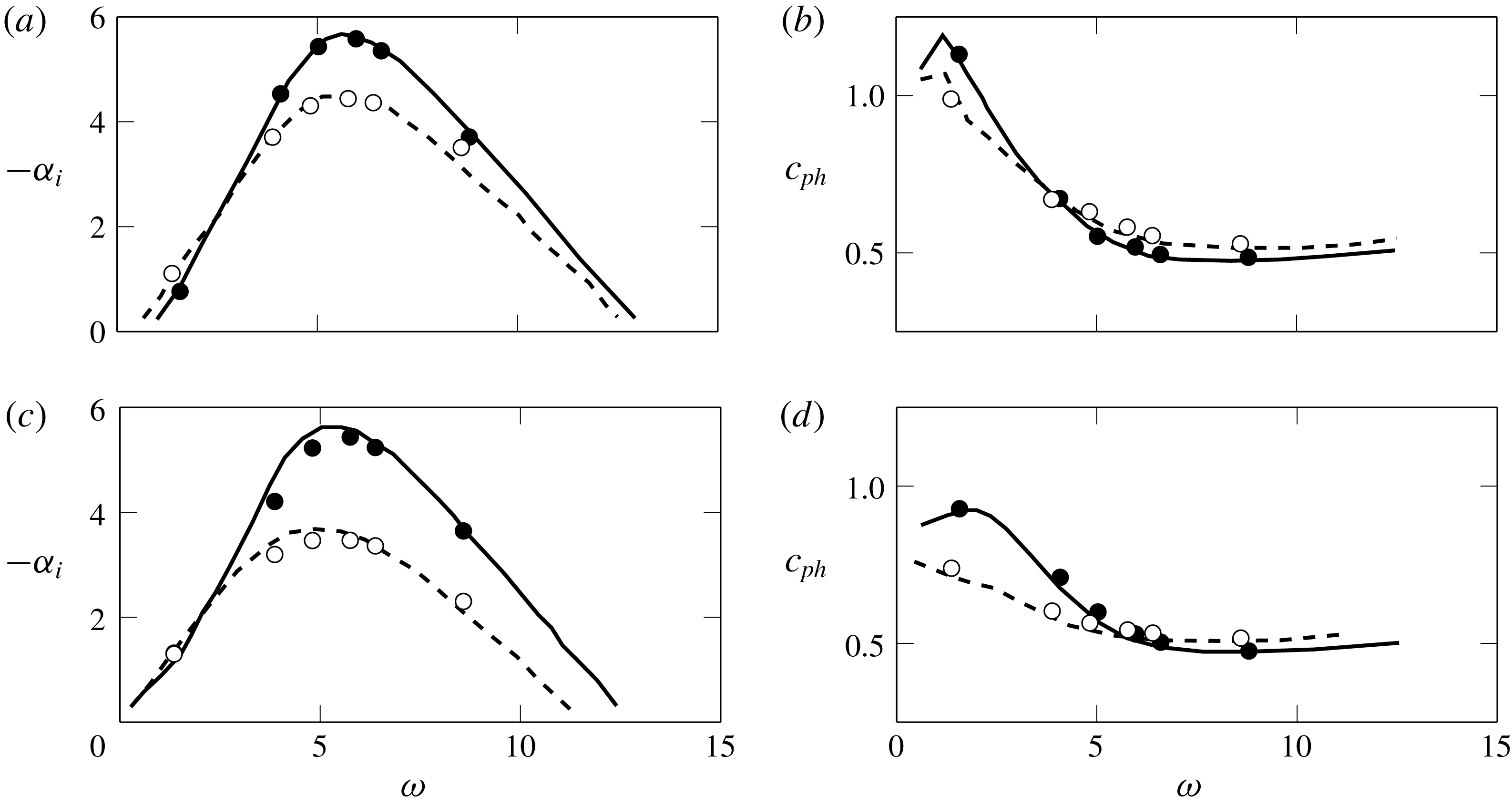
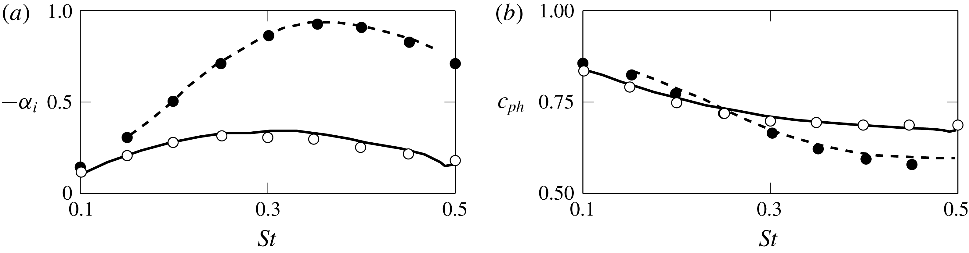
the jet exit velocity. A validation of the numerical approach is carried out by comparisons with Morris (Reference Morris1988) and Gudmundsson (Reference Gudmundsson2010), who have studied elliptic and serrated jets, respectively. Results are shown in figure 2 and figure 3 where we see a close match in growth rates and phase speeds of the most unstable mode found for each configuration.
Growth rate (a,c) and phase velocity (b,d) comparisons, for
 $ce_{0}$
(a,b) and
 $se_{1}$
(c,d) solutions, from
 $A/B=1.001$
(solid line) and
 $2.0$
(dashed) elliptic profiles given by Morris (Reference Morris1988). Here,
 $ce_{0}$
and
 $se_{1}$
stand for cosine elliptic and sine elliptic solutions related to the Mathieu functions, and
 $A/B$
is the ratio between the major and minor axes in the considered elliptic mean velocity profile. This notation is the same as that used by Morris (Reference Morris1988). Circles indicate the present results, and lines show results by Morris (Reference Morris1988).

Comparisons with growth rates (a) and phase velocities (b), at
 $x/D=2.0$
, for the SMC000 nozzle (dashed) and SMC001 nozzle (solid). Present numerical results are represented by the circles, and lines show results by Gudmundsson (Reference Gudmundsson2010).

3 Mean-flow parametrization
The streamwise mean velocity fields of two corrugated subsonic jets are considered. The first database consists of velocity measurements obtained from stereoscopic particle image velocimetry (PIV) by Bridges & Brown (Reference Bridges and Brown2004) in the Small Hot Jet Acoustic Rig (SHJAR) at NASA Glenn Research Center. These data correspond to mean velocity fields of a circular jet (nozzle SMC000) and a jet issuing from their SMC001 nozzle with
 $N=6$
chevrons. The nozzle exit diameter for the circular nozzle was 50.8 mm, whereas an equivalent diameter of 52.2 mm was reported for the SMC001 case using mass flow rate measurements. Both jets were operating at the same condition:
 $M_{\infty }=U_{j}/a_{\infty }=0.9$
,
 $T_{j}/T_{\infty }=0.85$
,
 $Re_{j}=16\times 10^{5}$
. Here,
 $T_{j}$
and
 $T_{\infty }$
are respectively the nozzle exit and ambient temperatures, and
 $Re_{j}$
is the jet exit Reynolds number, based on jet equivalent diameter.
The second database is of a jet with steady fluidic actuation reported by Maury et al. (Reference Maury, Cavalieri, Jordan, Delville and Bonnet2011), performed in the anechoic jet-noise facility ‘Bruit et Vent’ at the Centre d’Etudes Aérodynamiques et Thermiques (CEAT) in Poitiers. The round nozzle, with 80 mm diameter, operated at
 $M_{\infty }=0.42$
and
 $Re_{j}=7.4\times 10^{5}$
, and
 $N=8$
converging pairs of micro-jets (each with diameter
 $2.1$
mm) were applied around the circumference of the nozzle exit.
We limit the linear stability analysis to stations within the potential core, as these are expected to be dominated by modal solutions; non-modal behaviour was found to be more relevant further downstream (Tissot et al.
Reference Tissot, Zhang, Lajus, Cavalieri and Jordan2017). In fact, our subsequent results are going to show that the stability effects of azimuthal corrugation variation are only discernible in a region very near the nozzle exit. Thus, we focus our attention on three near-nozzle axial stations where experimental mean-flow data are available, viz.
 $x/D=0.5$
,
 $1.0$
and
 $2.0$
for the NASA data and
 $x/D=1.0$
,
 $1.5$
and
 $2.0$
for the Poitiers data. Prior to fitting the mean-flow field for the purpose of parametrization, its azimuthal periodicity is averaged over the
 $N$
equivalent azimuthal sectors. The hyperbolic tangent profile (Profile II) of Michalke (Reference Michalke1984)
 $$\begin{eqnarray}\displaystyle \bar{u}_{x}(r,\unicode[STIX]{x1D703})=\frac{M_{\infty }}{2}\left\{1+\tanh \left[0.5\frac{\boldsymbol{R}}{\unicode[STIX]{x1D723}}\left(\frac{\boldsymbol{R}}{r}-\frac{r}{\boldsymbol{R}}\right)\right]\right\}, & & \displaystyle\end{eqnarray}$$
is fitted to the mean axial velocity field along the radial direction at several azimuthal angles, thereby determining the two characteristic length scales. These two scales are: the radial position of the shear layer
 $\boldsymbol{R}$
(where
 $\bar{u}_{x}(\boldsymbol{R})=M_{\infty }/2$
) and the mixing-layer thickness
 $\unicode[STIX]{x1D6E9}$
. A second fit along azimuth was performed for these two identified parameters, by expanding them in respective cosine series.
 $$\begin{eqnarray}\displaystyle & \displaystyle \boldsymbol{R}(\unicode[STIX]{x1D703})=R_{0}\left(1+\mathop{\sum }_{j=1}^{\infty }A_{j}\cos (jN\unicode[STIX]{x1D703})\right), & \displaystyle\end{eqnarray}$$
 $$\begin{eqnarray}\displaystyle & \displaystyle \unicode[STIX]{x1D723}(\unicode[STIX]{x1D703})=\unicode[STIX]{x1D6E9}_{0}\left(1+\mathop{\sum }_{j=1}^{\infty }B_{j}\cos (jN\unicode[STIX]{x1D703})\right). & \displaystyle\end{eqnarray}$$
The Crocco–Busemann relation is used to determine the mean temperature and density fields from these velocity profiles (Michalke Reference Michalke1984).
In this form, we note that a zeroth-order approximation (only considering
 $R_{0}$
and
 $\unicode[STIX]{x1D6E9}_{0}$
) is a circular jet. It should be clear that these zeroth-order approximations are not equivalent to round nozzles, but instead correspond to an azimuthally-averaged corrugated jet. We will explore this feature later in our analysis, in order to distinguish between the influence of shear-layer thickness and azimuthal inhomogeneities, similar to what is done by Boujo, Fani & Gallaire (Reference Boujo, Fani and Gallaire2015) and Marant & Cossu (Reference Marant and Cossu2018) for the stability of shear layers with streaks. The inclusion of
 $A_{j}$
and
 $B_{j}$
terms, which can be seen as fractions multiplying
 $R_{0}$
and
 $\unicode[STIX]{x1D6E9}_{0}$
, introduces azimuthal variations with
 $2\unicode[STIX]{x03C0}/N$
periodicity.
The goodness of fit for the hyperbolic tangent profile is verified through R-square statistics, the worst cases being
 $0.9911$
for the SMC001, and
 $0.9942$
for the jet with micro-jets. For the cosine series, respectively for the jets with chevrons and micro-jets, the worst cases of R-square fits are
 $0.9438$
and
 $0.9980$
for
 $\boldsymbol{R}$
and
 $0.9488$
and
 $0.9986$
for
 $\unicode[STIX]{x1D723}$
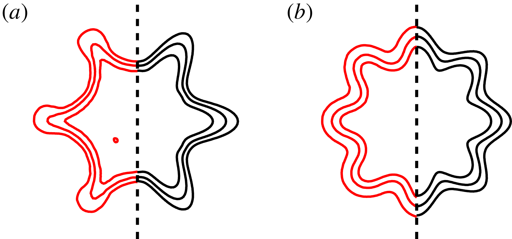
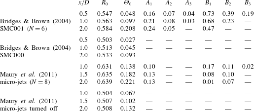
. Comparative results are shown in figure 4, highlighting that the proposed functional form represents fairly the velocity profiles of both jets. The fitting coefficients are presented in table 1. Values for the circular SMC000 and the circular counterpart of the jet with micro-jets are also included.
Comparison between original mean flows (red) and the extended hyperbolic tangent formulation (black), for the jet with chevrons (a) and with micro-jets (b).


Regarding the fitting coefficients for the SMC001 jet, we can observe in table 1 the pronounced increase in
 $\unicode[STIX]{x1D6E9}_{0}$
that this jet displays along the axial direction, when compared to the SMC000 case. This suggests that, (on average) chevrons are stabilizing the jet by the increase of mixing-layer thickness, which is known to decrease growth rates (Michalke Reference Michalke1984); however, the effect of azimuthal inhomogeneities should also be considered. For the sections near the nozzle, comparatively more terms (
 $A_{j}$
and
 $B_{j}$
) are found necessary to properly characterize the more localized corrugated structure of the jet profile. In this case, three terms were verified to be sufficient at
 $x/D=0.5$
, with smaller contributions from higher-order cosine terms (values below
 $1\,\%$
are disregarded). Further downstream, fewer terms need be considered, as the velocity profiles have smaller azimuthal variation. By comparing the leading-order coefficients,
 $A_{1}$
and
 $B_{1}$
, we see that large azimuthal variations occur in the shear-layer thickness
 $\unicode[STIX]{x1D723}$
(
 $73\,\%$
at
 $x/D=0.5$
and
 $47\,\%$
at
 $x/D=2.0$
), whereas the shear-layer position
 $\boldsymbol{R}$
has azimuthal oscillations of approximately
 $20\,\%$
consistently across the axial stations considered.
The action of steady micro-jet injection is also observed to mostly increase
 $\unicode[STIX]{x1D6E9}_{0}$
of the mean-flow field when compared to its circular counterpart, which also reinforces the idea that micro-jets similarly stabilize the jet by the increase of shear-layer thickness. In this case, however, the increase is followed by smaller
 $A_{j}$
and
 $B_{j}$
amplitudes (approximately
 $10\,\%$
), when compared to the SMC001. Further discussion on the corrugated mean flows from jets having chevrons or micro-jets can be found in Alkislar, Krothapalli & Butler (Reference Alkislar, Krothapalli and Butler2007).
4 Multiple unstable modes of corrugated jets
The base-flow parametrization of (3.1)–(3.3) is able to fit the mean-flow fields of both corrugated jets. In this work, we perform the analysis primarily by gradually varying the SMC001 chevron jet’s corrugation fit coefficients starting from zero (circular jet). These display greater amplitudes (corresponding to deeper corrugations) than their counterparts in the jet actuated by micro-jets, as shown in table 1. Thus, the results and conclusions from the chevron jet can be readily extended to the micro-jet actuated jet if one considers a flow with lower corrugation amplitudes. Moreover, given that the two jets have different Mach numbers, compressibility effects may be expected to be relevant. However, these differences are found to mostly follow the trends reported by Michalke (Reference Michalke1984), i.e. growth rates and phase speeds of low
 $St$
-modes are reduced at the higher Mach number. Specific results for the micro-jet actuated flow have been presented by Lajus et al. (Reference Lajus, Cavalieri and Deschamps2015).
4.1 Classification of modes based on continuation from circular jets
We first explore solutions of the linear stability problem for corrugated jets based on the analysis of the jet issuing from the SMC001 nozzle. This choice also allows direct comparison with corresponding results presented by Gudmundsson & Colonius (Reference Gudmundsson and Colonius2007) and Sinha et al. (Reference Sinha, Gudmundsson, Xia and Colonius2016a
). Growth rates
 $\unicode[STIX]{x1D6FC}_{i}$
and phase speeds
 $c_{ph}$
obtained for
 $\unicode[STIX]{x1D707}=0$
at
 $St=0.35$
are presented in figure 5. The continuous branch of critical-layer modes, with
 $\unicode[STIX]{x1D6FC}_{i}=0$
, which results from a singularity of the Rayleigh equation (2.11) whenever
 $\unicode[STIX]{x1D714}=\unicode[STIX]{x1D6FC}\bar{u}_{x}$
(Case Reference Case1960), can be seen along the real axis. However, since the behaviour of large-scale turbulent structures near the nozzle is expected to be dominated by unstable discrete modes, we will focus on these in what follows.
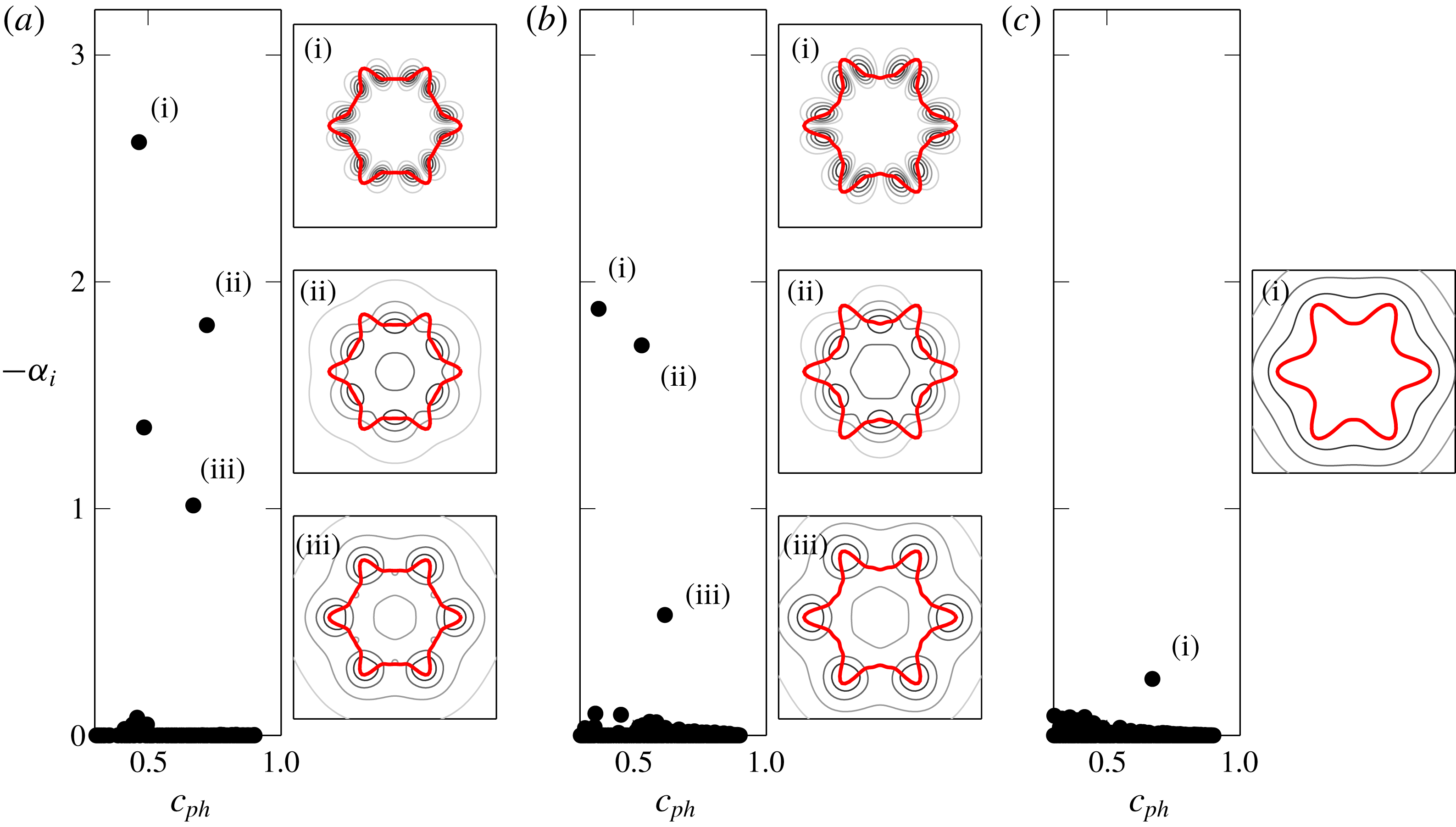
Eigenspectra of SMC001 at (a)
 $x/D=0.5$
, (b)
 $x/D=1.0$
and (c)
 $x/D=2.0$
, for
 $St=0.35$
. Pressure eigenfunctions are shown by their normalized absolute values, and are ordered by their magnitude of
 $-\unicode[STIX]{x1D6FC}_{i}$
. Thick red curves represent the base-flow axial velocity contour at
 $\bar{u}_{x}=0.5$
.

Multiple unstable solutions (discrete) are found near the nozzle region (
 $x/D=0.5$
and
 $1.0$
), but only one unstable mode is obtained further downstream (
 $x/D=2.0$
). These are mostly in good agreement with previous studies (Gudmundsson & Colonius Reference Gudmundsson and Colonius2011; Sinha et al.
Reference Sinha, Gudmundsson, Xia and Colonius2016a
), especially modes (ii) and (iii). The associated eigenfunctions are also consistent with the results of the cited works, with some peaking at the lobes of the base flow and others at the flats. Mode (i) that appears at the first two stations are not reported by previous studies.
Our goal is to trace the origin of these multiple modes, by exploring the features of our base-flow parametrization. By continuously varying the fitted
 $A_{j}$
and
 $B_{j}$
(simultaneously) with a perturbation factor (
 $P$
) between
 $0$
and
 $1.3$
, such that
 $$\begin{eqnarray}\displaystyle & \displaystyle \boldsymbol{R}(\unicode[STIX]{x1D703})=R_{0}\left(1+P\mathop{\sum }_{j=1}^{\infty }A_{j}\cos (jN\unicode[STIX]{x1D703})\right), & \displaystyle\end{eqnarray}$$
 $$\begin{eqnarray}\displaystyle & \displaystyle \unicode[STIX]{x1D723}(\unicode[STIX]{x1D703})=\unicode[STIX]{x1D6E9}_{0}\left(1+P\mathop{\sum }_{j=1}^{\infty }B_{j}\cos (jN\unicode[STIX]{x1D703})\right), & \displaystyle\end{eqnarray}$$
we can track the solution behaviour as a continuation of corresponding ones for circular jets. Note that
 $P=1$
stands for the original base flow of the SMC001 jet with chevrons, but smaller
 $P$
values are also found to approximate the base-flow coefficients of the jet with micro-jets (from table 1). Thus,
 $P$
can be seen as a metric for corrugation amplitude, which can be continuously varied from a circular (azimuthally averaged) jet to increased corrugated profiles. Results are shown in figure 6, for
 $x/D=0.5$
,
 $1.0$
and
 $2.0$
.
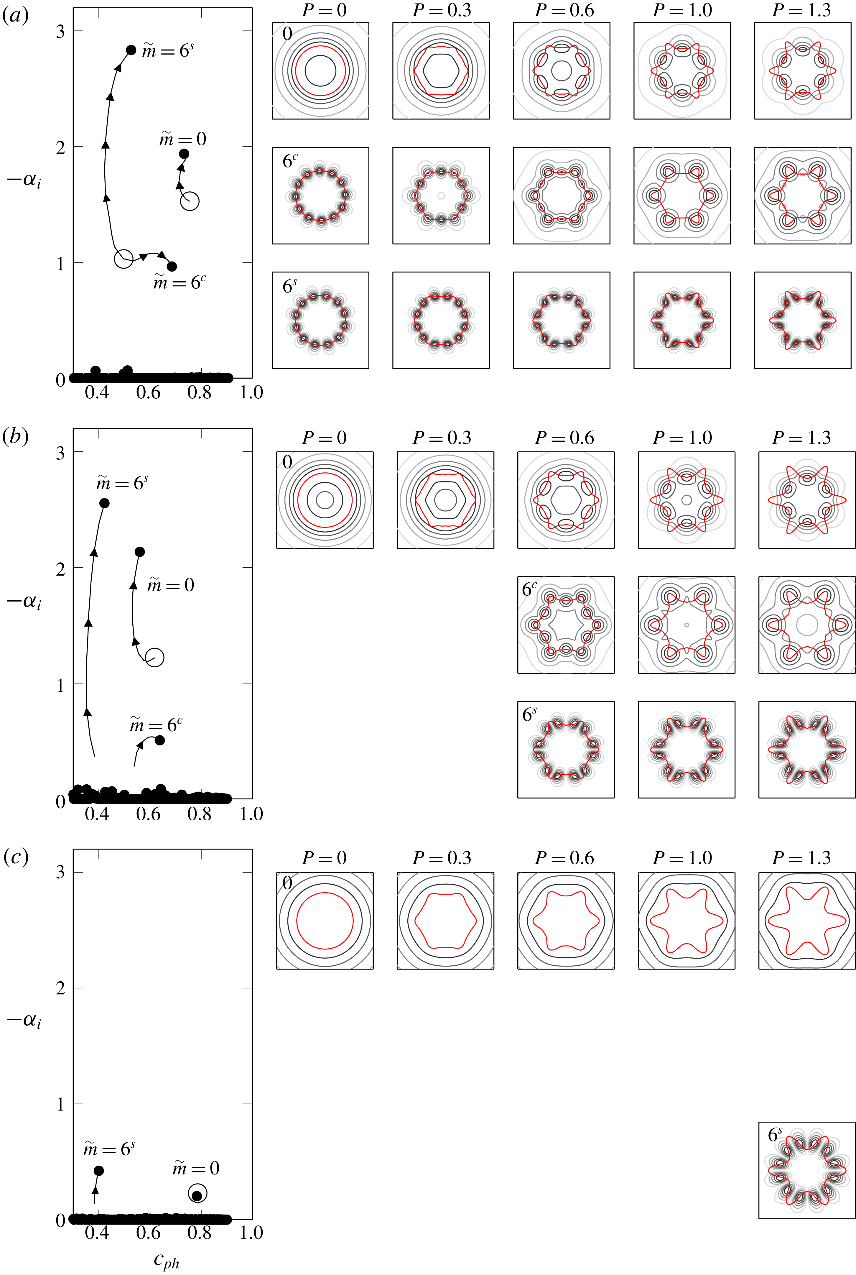
Eigensolution branches traced with gradual increase of azimuthal corrugation parameter
 $P$
of (4.1)–(4.2) at
 $x/D=0.5$
(a),
 $1.0$
(b) and
 $2.0$
(c), for
 $St=0.35$
. Open circles are results for
 $P=0$
, whereas end dots are results for
 $P=1.3$
. Arrows indicate directions of increasing
 $P$
. Presentation of eigenfunctions follows the scheme of figure 5.

The starting points are solutions obtained for
 $P=0$
. For such circular jets, azimuthal wavenumbers
 $m=0$
and
 $m=\pm 6$
possess unstable Kelvin–Helmholtz modes for sufficiently thin shear layers. Such modes are contained in the
 $\unicode[STIX]{x1D707}=0$
Floquet ansatz, and are represented in figure 6 with open circles; notice that
 $m=-6$
and
 $6$
have the same eigenvalue (in
 $x/D=0.5$
), and are thus degenerate eigenfunctions. As small azimuthal inhomogeneities are included (
 $P\ll 1$
), we verify the break up of the
 $m=\pm 6$
degeneracy. Such behaviour was observed analytically by Kopiev et al. (Reference Kopiev, Ostrikov, Chernyshev and Elliott2004), and we expect it to be a common feature in both corrugated jets considered here. Since eigenfunctions for
 $P>0$
can no longer be associated with a single azimuthal wavenumber
 $m$
, we identify these solutions according to the azimuthal mode from which they emerge (now labelled as
 $\tilde{m}$
) and whether the (pressure) eigenfunction has peaks aligned with the lobes (referred to with superscript ‘
 $c$
’) or flats (superscript ‘
 $s$
’), making reference to their cosinusoidal and sinusoidal character (Morris & Miller Reference Morris and Miller1984; Koshigoe & Tubis Reference Koshigoe and Tubis1986). Thus the
 $\tilde{m}=0$
mode refers to the continuation of the axisymmetric mode of circular jets (
 $P=0$
) for corrugated ones (
 $P>0$
), and
 $\tilde{m}=6^{c}$
and
 $6^{s}$
refer to the continuations of the
 $m=\pm 6$
modes. The solutions for
 $m=\pm 6$
are not visible at
 $x/D=1.0$
and
 $2.0$
for
 $P=0$
, but their continuations become apparent after some level of perturbation (
 $P=0.5$
and
 $P=1.1$
, respectively), forming similar paths to those found in
 $x/D=0.5$
. We thus conclude that these modes are stable for
 $P=0$
at these stations, and cannot be found as solutions of the Rayleigh equation, unless a deformation of the integration contour is taken to avoid the critical-layer singularity (Tam & Morris Reference Tam and Morris1980; Boyd Reference Boyd1985).
These results highlight that the multiple unstable modes obtained for non-circular jets, seen in previous studies (Gudmundsson & Colonius Reference Gudmundsson and Colonius2007; Sinha et al.
Reference Sinha, Gudmundsson, Xia and Colonius2016a
), are all related to the Kelvin–Helmholtz mechanism, as they can be tracked from the standard Kelvin–Helmholtz modes of circular jets. The multiple unstable modes are simple continuations of circular jet modes, keeping in mind that all eigenfunctions that are consistent with the Floquet ansatz for a jet with
 $N$
corrugations should be tracked. For the present base flow, with
 $N=6$
corrugations, three unstable modes were seen to be continuations of
 $m=0$
and
 $\pm 6$
Kelvin–Helmholtz modes of the corresponding azimuthally averaged jet.
In general, these gradual base-flow deformations are observed to be more significant at stations
 $x/D=0.5$
and
 $1.0$
, promoting higher growth rates for modes
 $\tilde{m}=6^{s}$
, but with minor variations of their phase velocity. Conversely, modes
 $\tilde{m}=6^{c}$
are found to increase their phase speeds for higher
 $P$
, but without much variation in growth rates. Solutions for
 $\tilde{m}=0$
are found to become more unstable with increasing
 $P$
, presenting minor variations in their phase velocities. The exceptions here are small values of
 $P$
at
 $x/D=1.0$
and the results further downstream, at
 $x/D=2.0$
Regarding the eigenfunction shape, an increase in the base-flow deformation has a significant effect on the eigenfunctions for the
 $\tilde{m}=0$
and
 $\tilde{m}=6^{c}$
modes, with the former becoming less axisymmetric and the latter becoming more so. Such redistribution of azimuthal coherence suggests that, in principle, both
 $\tilde{m}=0$
and
 $\tilde{m}=N^{c}$
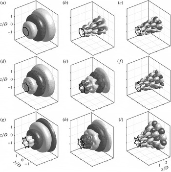
should be considered as acoustically relevant structures in corrugated jet profiles. The streamwise evolution of the pressure fluctuations is illustrated in figure 7, from solutions obtained at
 $x/D=0.5$
applied to (2.4). We have presented the magnitudes of the pressure eigenfunction in all other figures; here we depict isocontours of their real part to better represent the wavepacket shape in the near-nozzle region.
Reconstructed pressure disturbances for (a,d,g)
 $\tilde{m}=0$
, (b,e,h)
 $\tilde{m}=6^{c}$
and (c,f,i)
 $\tilde{m}=6^{s}$
. Representative positive and negative of the real part of the pressure (
 $\pm 0.5$
, normalized values). Results obtained for
 $P=0.3$
(a–c),
 $0.6$
(d–f) and
 $1.3$
(g–i). The base flow is indicated by the
 $\bar{u}_{x}=0.5$
contour.

Another feature observed in these solutions is that at
 $x/D=0.5$
, the modes forming the
 $\tilde{m}=0$
branch peak at the base-flow flats, while those for
 $\tilde{m}=6^{c}$
appear to evolve from something similar to the original
 $m=\pm 6$
shape, at small
 $P$
, to modes that are more axisymmetric with peaks occurring at the base-flow peaks. Solutions at
 $x/D=2.0$
behave in the opposite manner, with the increase of
 $P$
modifying the eigenfunction shape of
 $\tilde{m}=0$
to those with peaks aligned with the base-flow peaks. This will be further investigated in what follows.
Saddles for perturbed profiles at (a)
 $x/D=0.5$
and (b)
 $x/D=1.0$
, formed by
 $\tilde{m}=0$
(blue) and
 $\tilde{m}=6^{c}$
(red) defined at
 $P\ll 1$
. Arrows indicate direction of increased
 $P$
, with equally spaced steps of
 $0.1$
, from
 $0$
to
 $1.3$
. For fixed
 $P$
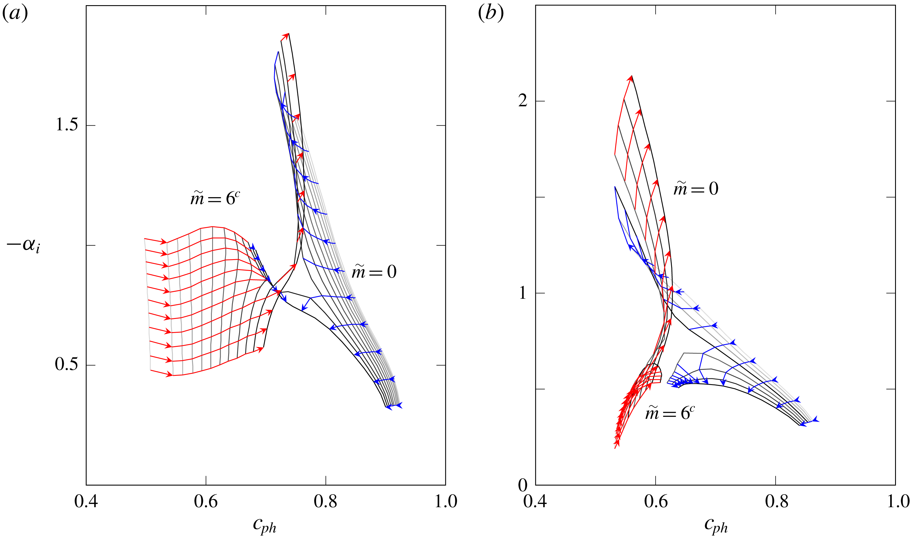
, the grey lines show the trajectory of the modes as frequency is increased from
 $St=0.15$
to
 $0.35$
(from bottom to top).

4.2 Axis switching of eigenfunctions of unstable modes
The complex behaviour of the eigenfunctions for the
 $\tilde{m}=0$
and
 $\tilde{m}=6^{c}$
modes can be understood as an axis switching that occurs when these two modes form a saddle in the complex
 $\unicode[STIX]{x1D6FC}$
plane as the (real) frequency is varied. Figure 8 shows that at both
 $x/D=0.5$
and
 $x/D=1.0$
, a saddle is formed and the two modes exchange their identities at the saddle. This is similar to what has been found as the temperature ratio in a round jet is varied (Michalke Reference Michalke1970), which was later found to be related to the occurrence of absolute instability in hot jets (Huerre & Monkewitz Reference Huerre and Monkewitz1985). In that case, however, the saddle is formed by two solutions whose group velocities are in the opposite directions, which is not expected to be the case here. Indeed, by application of the Briggs criterion (Briggs Reference Briggs1964; Huerre et al.
Reference Huerre, Batchelor, Moffatt and Worster2000), we confirmed that all these discrete unstable solutions comprise downstream propagating waves, and thus are not related to absolute instability. Saddles formed by two downstream travelling waves also appear in high supersonic cold jets, where the Kelvin–Helmholtz mode blends itself with supersonic instability wave modes (Tam & Hu Reference Tam and Hu1989).
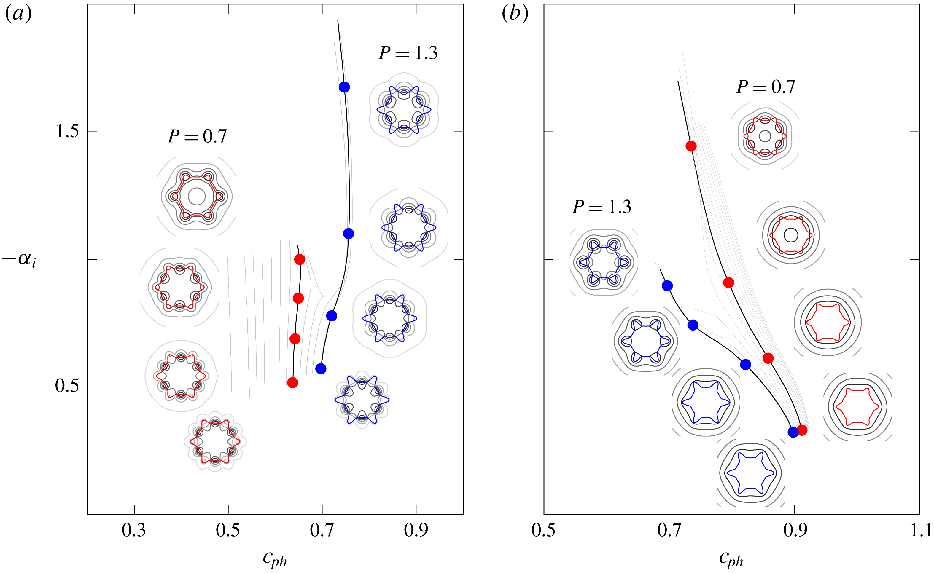
A peculiarity related to eigenfunctions of the two saddle modes is shown in figure 9. At very low
 $St$
values,
 $\tilde{m}=0$
closely follows the base-flow shape, while
 $\tilde{m}=6^{c}$
tends to present peaks at the flats. For situations where
 $P<1.1$
in
 $x/D=0.5$
(and
 $P<1.0$
in
 $x/D=1.0$
), the increase of
 $St$
is followed by the switch of behaviour between these two solutions, which alters the azimuthal location of their peaks; this can be thought of an axis switching of eigenfunctions. For higher
 $P$
this is not observed, but then an exchange of the solutions trajectories occurs, with
 $\tilde{m}=6^{c}$
taking similar paths to previous
 $\tilde{m}=0$
solutions, and vice versa. One should observe that the gradual perturbations at a fixed
 $St=0.35$
, shown in figure 6, are therefore not restricted to a single mode continuation along
 $\tilde{m}=0$
and
 $\tilde{m}=6^{c}$
branches. Our mode classification thus follows the azimuthal mode continuation found at lower
 $St$
. Please note the supplemental material that is made available in the online version of the paper at https://doi.org/10.1017/jfm.2019.573.
Axis switching of solutions near the saddle point in
 $x/D=0.5$
, for
 $\tilde{m}=6^{c}$
(a) and
 $\tilde{m}=0$
(b). Branches of
 $P=0.7$
(red) and
 $1.3$
(blue) are emphasized, showing the eigenfunctions for
 $St=0.15$
,
 $0.2$
,
 $0.25$
and
 $0.3$
from bottom to top.

5 Stability implications of mean-flow changes
Some systematic base-flow changes are now considered, in order to quantify the resulting growth rates and phase speeds of
 $\tilde{m}=0$
and
 $6^{c}$
. We restricted our attention to these two modes because the relatively axisymmetric structure of their eigenfunctions would presumably lead to a more efficient radiation of sound (Jordan & Colonius Reference Jordan and Colonius2013). Additionally, we focus on those aspects of the base flow that would reduce either the growth rate and/or phase speed as this would tend to reduce their radiation efficiency (Kœnig et al.
Reference Kœnig, Sasaki, Cavalieri, Jordan and Gervais2016). For later comparison, results for the (circular) zeroth-order approximations at
 $x/D=0.5$
and
 $2.0$
are first shown separately in figure 10, where the
 $m=0$
and
 $m=\pm 6$
modes are highlighted.
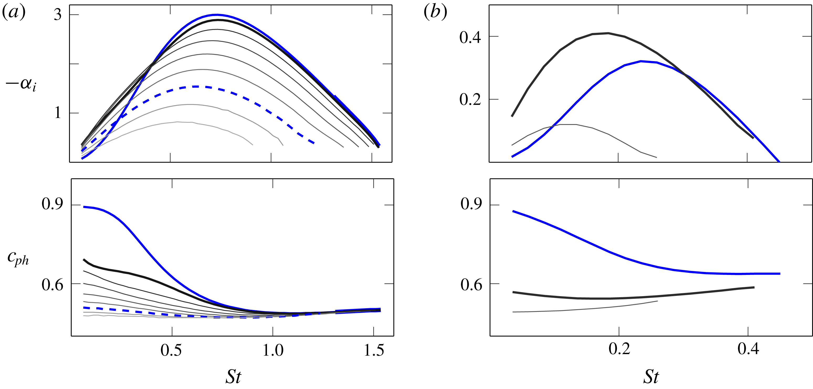
Growth rates (top) and phase speeds (bottom) obtained for the zeroth-order approximation at (a)
 $x/D=0.5$
and (b)
 $x/D=2.0$
. Blue lines highlight
 $m=0$
(solid) and
 $m=\pm 6$
(dashed). Others are coloured by increasing azimuthal wavenumber (black
 $m=\pm 1$
, lightest grey
 $m=\pm 8$
)

5.1 Azimuthal inhomogeneities of
 $\boldsymbol{R}$
and
$\unicode[STIX]{x1D723}$


The variation in growth rate and phase speed as
 $P$
is varied are shown in figure 11. Recall that varying
 $P$
alters the magnitude of the azimuthal inhomogeneity, and thus, for instance, mimics the effect of chevron penetration (Bridges & Brown Reference Bridges and Brown2004); however, one should bear in mind that increasing penetration is, in a real jet, invariably accompanied by higher azimuthally averaged shear-layer thickness
 $\unicode[STIX]{x1D6E9}_{0}$
. In the present analysis we are able to isolate these two effects. We concentrate on the azimuthal variation aspect of penetration only, as the effect of increasing shear-layer thickness is well understood to be stabilizing (Michalke Reference Michalke1984).
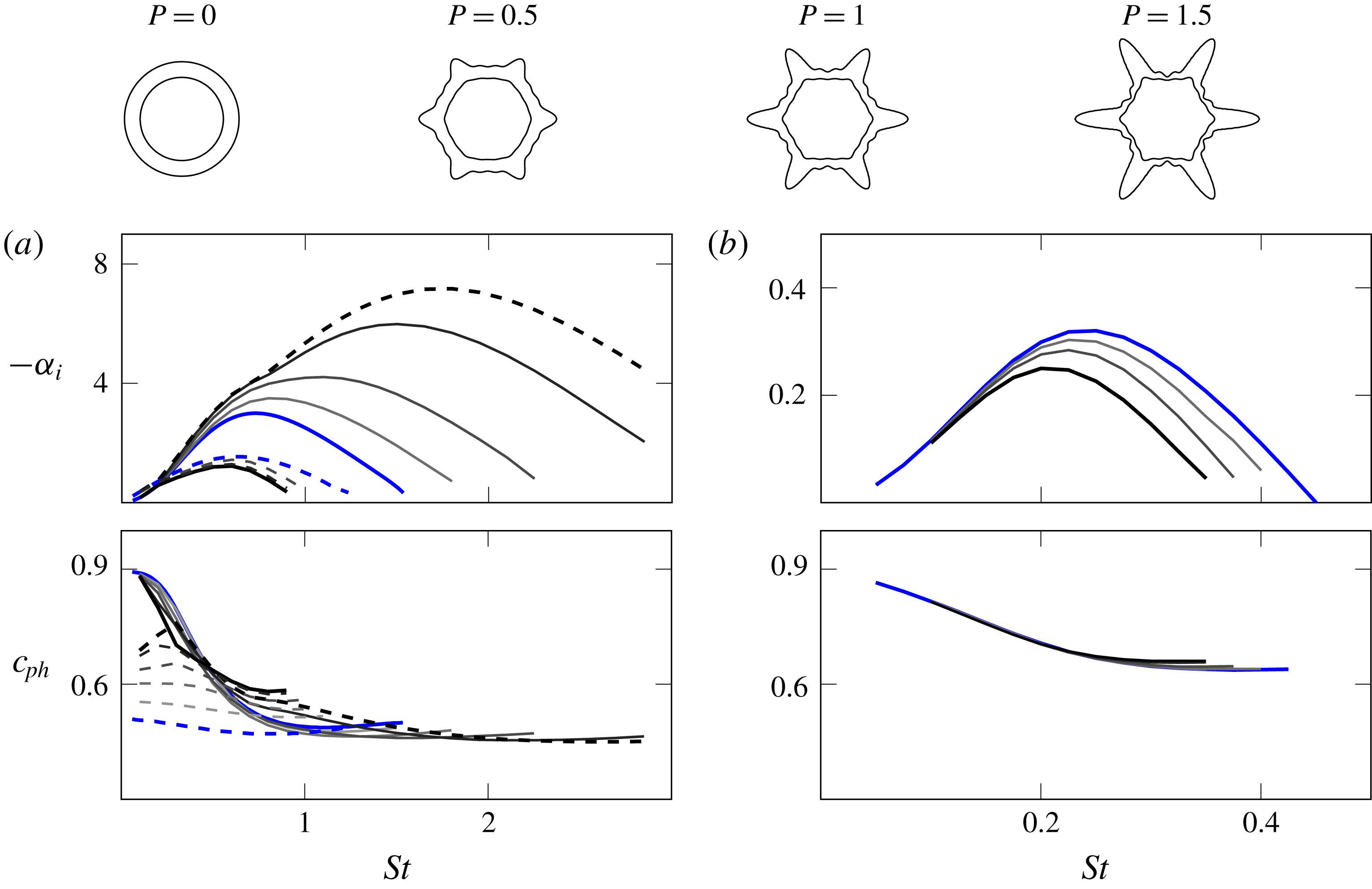
In the near-nozzle region (refer to figure 11
a), we notice that the growth rates and the range of unstable frequencies change more significantly for
 $\tilde{m}=0$
, and that increasing
 $P$
is destabilizing for this mode; for
 $\tilde{m}=6^{c}$
there are only mild changes in growth rate induced by azimuthal inhomogeneities in the base flow. The tendency is mostly monotonic with
 $P$
, until an exchange of
 $\tilde{m}=0$
and
 $\tilde{m}=6^{c}$
(in
 $P\geqslant 1.1$
) due to a saddle around
 $St\approx 0.2$
. On the other hand, regarding phase speeds,
 $\tilde{m}=6^{c}$
is observed to be the most affected mode. Dominant unstable solutions (those with highest growth rate) are found to closely follow phase velocities obtained from the zeroth-order approximations. Downstream (see figure 11
b), growth rates of mode
 $\tilde{m}\,=\,0$
are slightly reduced, which is opposite to what is seen near the nozzle. Phase speeds are nearly insensitive to the increase of
 $P$
.
Further investigation is carried out to ascertain the effect of the applied azimuthal inhomogeneities in a more decoupled manner. By imposing
 $B_{j}=0$
in (3.3), the perturbations are isolated in the
 $\boldsymbol{R}$
term. Conversely, by enforcing
 $A_{j}=0$
, azimuthal variations are confined to
 $\unicode[STIX]{x1D723}$
. The results for the individual influence of
 $\boldsymbol{R}$
and
 $\unicode[STIX]{x1D723}$
are shown in figures 12 and 13, respectively.
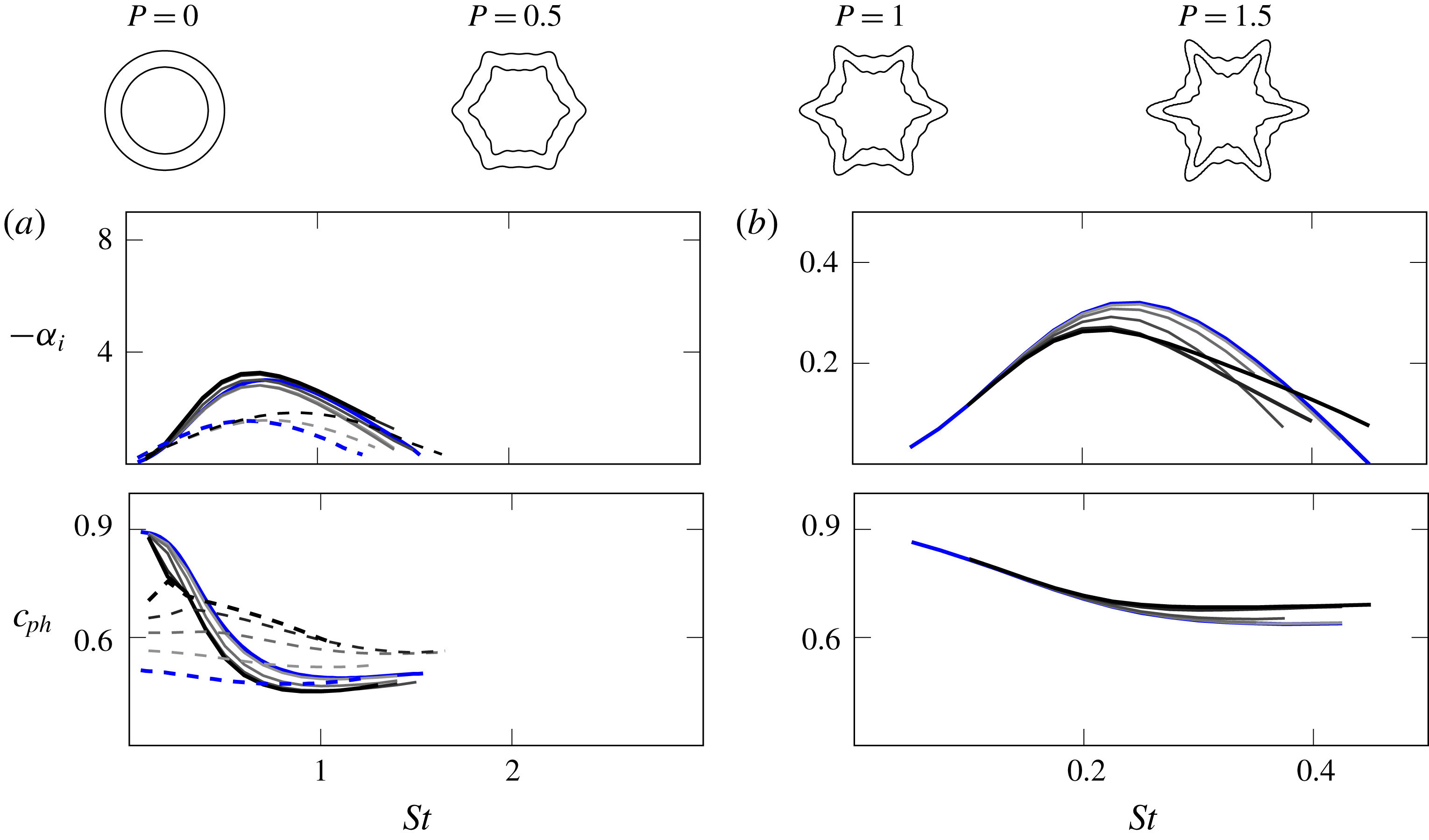
Top: base-flow deformation, iso-lines for
 $M=0.9$
and
 $0.1$
. Growth rates and phase speeds for perturbed
 $P$
(a) near the nozzle,
 $x/D=0.5$
and (b) downstream,
 $x/D=2.0$
. Solid lines are
 $\tilde{m}=0$
and dashed
 $\tilde{m}=6^{c}$
, coloured by increasing
 $P$
within the range:
 $0.25$
,
 $0.5$
,
 $0.75$
,
 $1.0$
and
 $1.1$
(lightest grey
 $P=0.25$
, black
 $P=1.1$
). Zeroth-order results are solid blue for
 $m=0$
and dashed blue for
 $m=\pm 6$
.

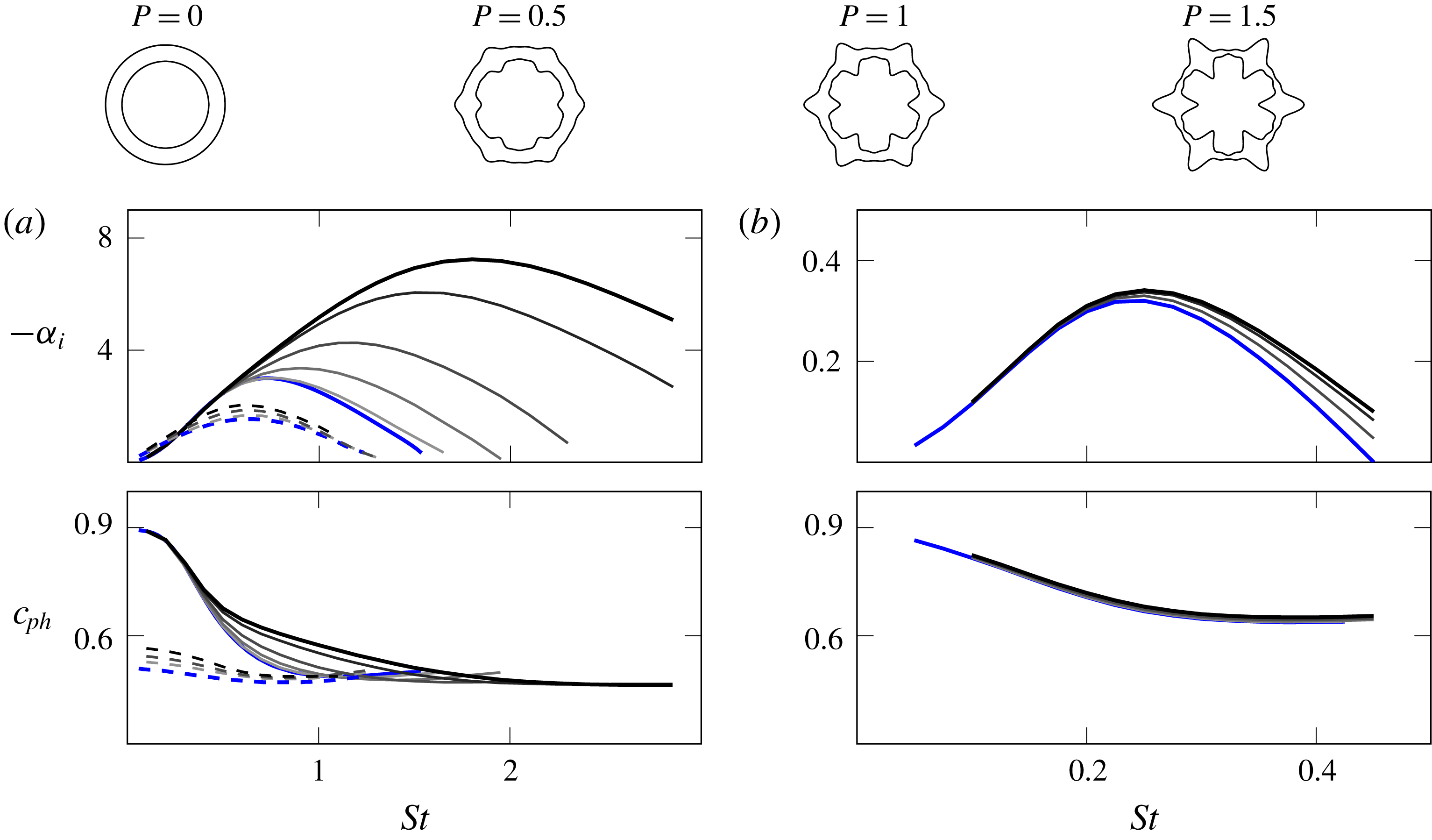
Growth rates and phase speeds for the
 $\boldsymbol{R}$
effect (a) near the nozzle and (b) downstream. Solid lines are
 $\tilde{m}=0$
and dashed
 $\tilde{m}=6^{c}$
. Coloured by increasing
 $P$
, within the range:
 $0.25$
,
 $0.5$
,
 $0.75$
,
 $1.0$
and
 $1.1$
(lightest grey
 $P=0.25$
, black
 $P=1.1$
). Zeroth-order results are shown in solid blue lines for
 $m=0$
and dashed for
 $m=\pm 6$
.

Growth rates and phase speeds for the
 $\unicode[STIX]{x1D723}$
effect (a) near the nozzle and (b) downstream. Solid lines are
 $\tilde{m}=0$
and dashed
 $\tilde{m}=6^{c}$
. Coloured by increasing
 $P$
, within the range:
 $0.25$
,
 $0.5$
,
 $0.75$
,
 $1.0$
and
 $1.1$
(lightest grey
 $P=0.25$
, black
 $P=1.1$
). Zeroth-order results are shown in solid blue lines for
 $m=0$
and dashed for
 $m=\pm 6$
.

Interestingly, the
 $\boldsymbol{R}$
effect seems to control the change in phase speed observed in the combined
 $\boldsymbol{R}/\unicode[STIX]{x1D723}$
effect, but with little change in growth rate, whereas
 $\unicode[STIX]{x1D723}$
variation has the opposite effect. In both cases the changes are pronounced at
 $x/D=0.5$
, but by
 $x/D=2.0$
the phase speeds and growth rates are again insensitive to
 $\boldsymbol{R}$
and
 $\unicode[STIX]{x1D723}$
modulations applied independently, as they were when applied in unison.
5.2 Flow periodicity
$N$

Similar to penetration, the effect of increasing the number of corrugations in real jets may be accompanied by a total increase of the azimuthally averaged mixing-layer thickness
 $\unicode[STIX]{x1D6E9}_{0}$
(Bridges & Brown Reference Bridges and Brown2004). Again, our focus is restricted to the azimuthal variations. In order to investigate the influence of base-flow periodicity, all fit results for the SMC001 nozzle from table 1 are maintained fixed, while the number of identical domain corrugations
 $N$
is varied. This has the outcome that more modes appear together, especially when larger pieces of the flow domain are considered. Our attention is restricted to
 $\tilde{m}=0$
and
 $N^{c}$
(here only considering
 $8^{c}$
, as it overtakes
 $\tilde{m}=0$
). Results are shown in figure 14.
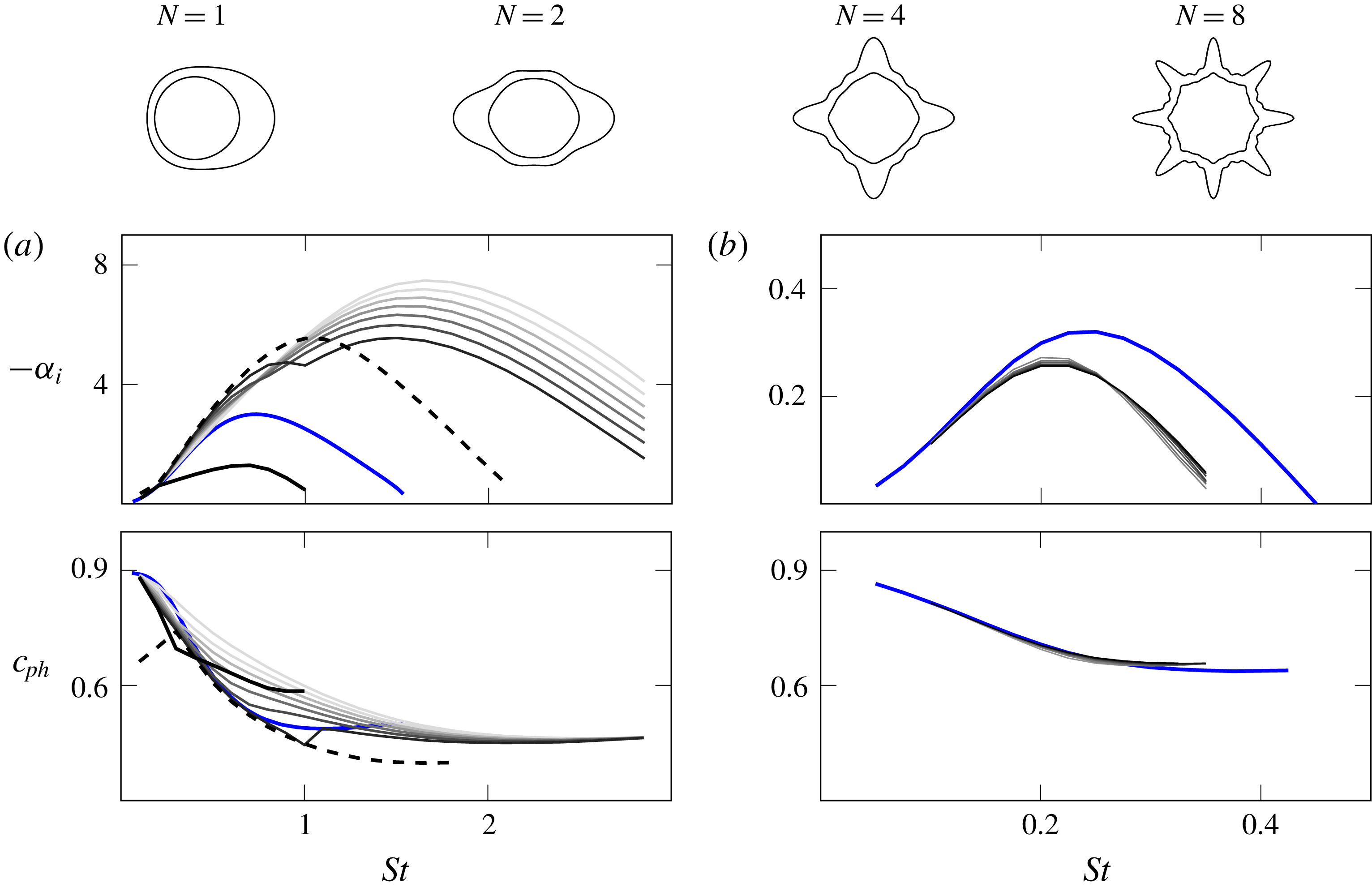
Growth rates and phase speeds for varying
 $N$
(a) near the nozzle region and (b) downstream. Solid lines are
 $\tilde{m}=0$
and dashed
 $\tilde{m}=N^{c}$
. Colours are for increasing
 $N$
, within the range:
 $1$
,
 $2$
,
 $3$
,
 $4$
,
 $5$
,
 $6$
,
 $7$
and
 $8$
(lightest grey
 $N=1$
, black
 $N=8$
). Zeroth-order results are shown in solid blue lines for
 $m=0$
.

The increase of
 $N$
is found to mostly reduce growth rates and phase speeds of the dominant unstable solutions in the near-nozzle region. There is an apparent trade-off in growth rates, increasing with
 $N$
(when
 $St<0.7$
) and decreasing (when
 $St>0.7$
). Such behaviour is related to a second saddle, between
 $\tilde{m}=0$
and
 $2N^{c}$
(not shown here), that appears with further increase of
 $N$
(around
 $N\geqslant 7$
). The behaviour of these modes around the saddle mostly follows the findings from § 4.2, and for this reason is not further discussed. For the downstream region, solutions are again found to be quite robust, depending only weakly on the number of corrugations.
6 Discussion
Before the concluding remarks, some additional comments are made here in order to clarify the underlying assumptions in our theoretical analysis. We follow with a brief discussion on how we expect our results to be relevant for non-circular jet stability and aeroacoustics.
6.1 Connection of parallel-flow results with wavepackets in slowly diverging jets
First, there is the assumption of locally parallel base flow. Usually, if the streamwise jet development is slow over an instability wavelength, one can assume that perturbations at any streamwise station develop as if the base flow were locally parallel. This does not seem to be the case here, as significant changes in the stability properties can be noticed within a short distance from the jet nozzle, thus calling into question the validity of the parallel-flow assumption. An alternative perspective, however, is given when we consider the locally parallel assumption as a zeroth-order approximation of an asymptotic series expansion, where the spread rate of the flow is taken as the small-scale parameter. Using the method of multiple scales, the zeroth-order solution becomes the parallel-flow result, with a free amplitude whose spatial distribution is obtained by a solvability condition found in the higher-order equations (Crighton & Gaster Reference Crighton and Gaster1976; Tam & Morris Reference Tam and Morris1980). This in turn leads to the ansatz used in the parabolized stability equations. Indeed, the close agreement obtained by Sinha et al. (Reference Sinha, Gudmundsson, Xia and Colonius2016a ) between PSE solutions and experiments and simulations of serrated jets supports the applicability of linear stability theory to corrugated jets.
One important consequence of the linear parallel system, however, is that acoustic and instability-related wave solutions appear decoupled by the homogeneity along the axial direction. It is only when the jet becomes non-parallel, or when the perturbation amplitude reaches a level that triggers nonlinearity, that acoustic and instability modes may become coupled in this framework (Jordan & Colonius Reference Jordan and Colonius2013). By assuming a locally parallel flow and undertaking the investigation only on azimuthal inhomogeneities, we have restricted our attention strictly to the changes in instability waves promoted by corrugations. If one were to model the jet spread, the acoustic implications of the results would have been clearer. Some modes possibly have better acoustic efficiency than others. In principle, both
 $\tilde{m}=0$
and
 $\tilde{m}=N^{c}$
are candidate solutions expected to be relevant for the noise radiation due to their quasi-axisymmetric shape (Michalke Reference Michalke1970; Michalke & Fuchs Reference Michalke and Fuchs1975), as discussed in § 4.1. The influence of the saddle studied in § 4.2 on the radiating noise, however, is more difficult to predict. A more definitive determination would require analysis of well-resolved experimental or simulation data that are unfortunately unavailable at present. Here we are restricted to an indirect assessment of the acoustic relevance of our results, invoking their well-established connection with the Kelvin–Helmholtz modes found at the near-nozzle region. In this perspective, reducing growth rates and phase speeds are expected to lead to noise reduction (Jordan & Colonius Reference Jordan and Colonius2013; Kœnig et al.
Reference Kœnig, Sasaki, Cavalieri, Jordan and Gervais2016), if properties such as wavepacket jitter or coherence decay (Cavalieri et al.
Reference Cavalieri, Jordan, Agarwal and Gervais2011; Cavalieri & Agarwal Reference Cavalieri and Agarwal2014; Baqui et al.
Reference Baqui, Agarwal, Cavalieri and Sinayoko2015) are not affected.
Although the peak noise is related to axially extended wavepackets, going beyond the jet potential core, these are crucially determined by their near-nozzle instability characteristics. Our analysis shows that the stability effects of corrugated base flows are limited to a region very near the nozzle; however, downstream profiles, are still influenced by the nozzle serrations, as their averaged shear-layer thickness
 $\unicode[STIX]{x1D6E9}_{0}$
is larger than what is seen for a circular nozzle. For our results, despite low azimuthal inhomogeneities for the serrated nozzle at
 $x/D=2$
, its averaged shear-layer thickness is considerably larger than the SMC000 result, as shown in table 1. Such differences persist downstream of the potential core, as shown by Sinha et al. (Reference Sinha, Gudmundsson, Xia and Colonius2016a
). Hence, the effect of nozzle serrations in jet stability should be felt throughout the development of wavepackets; in the near-nozzle region azimuthal inhomogeneities should play an important role, but at downstream locations the higher momentum thickness would still impact wavepacket growth rates and phase speeds.
6.2 Relationship of present findings with previous experiments on jet noise
We may now attempt to connect the stability results with experimental results of jets with chevrons or micro-jets, mostly to discuss the effect of corrugations on the radiated noise. From comparisons between the fit coefficients displayed in table 1, it seems that noise reduction is achieved by an (averaged) increase of mixing-layer thickness in both jets. However, when azimuthal inhomogeneities are included, such as in figure 11, a slight reduction of phase speed is observed for low
 $St$
, together with a large increase in growth rates, especially for higher
 $St$
, in the region closest to the nozzle. This may explain the experimentally observed trade-off encountered between noise reduction at lower frequencies and increase at higher ones with increasing chevron penetration (Bridges & Brown Reference Bridges and Brown2004; Alkislar et al.
Reference Alkislar, Krothapalli and Butler2007).
An interesting result is found in figure 12, where we introduced increasing azimuthal perturbations of the radial position of the shear layer keeping its thickness homogeneous. This approximately follows the observed base-flow changes of the jet actuated with micro-jets. Results for this investigation show a progressive decrease of the phase speed of the
 $\tilde{m}=0$
instability for higher oscillations of radial position, but without any high-frequency penalty associated with higher growth rates. This may be related to the observation that micro-jets lead to much less significant high-frequency noise (Alkislar et al.
Reference Alkislar, Krothapalli and Butler2007), once we disregard much of its high-frequency content that is apparently related to the injectors themselves (Callender, Gutmark & Martens Reference Callender, Gutmark and Martens2007). However, a definitive confirmation of this theoretical result requires a more empirical investigation.
It is more difficult to establish the practical connection of our analysis of the stability implications of the number of corrugations. Bridges & Brown (Reference Bridges and Brown2004) reported that increasing the chevron count thickens the mixing layer while reducing the azimuthal variations of the jet mixing layer, and that this is linked to a reduction of the radiated noise. In our analysis, on the other hand, the mixing-layer thickness parameter was retained constant when the number of corrugations was increased, precluding any conclusion regarding its noise benefits. Thus, this portion of the analysis is included solely for theoretical completeness of the parametric investigation.
We conclude this section by reiterating how this study represents a preliminary step towards the creation of a theoretical framework for the design of corrugated nozzles focusing on their possible aeroacoustic benefit. Our work is also a significant contribution to the rather limited literature on the research of instability waves in non-circular jets (Gutmark & Grinstein Reference Gutmark and Grinstein1999; Morris Reference Morris2010). The need for additional computational and experimental data to confirm the findings is evident, and constitutes a natural continuation of this line of investigation.
7 Conclusion
In this paper we have investigated the instability wave characteristics of corrugated subsonic jets, within the assumption of locally parallel base flows. Floquet theory is applied to the compressible Rayleigh equation in order to explore the azimuthally periodic base flow. We parametrized mean-flow fields of corrugated jets by introducing a cosine series expansion of the azimuthal variation of their two characteristic length scales – the radial position of the shear layer
 $\boldsymbol{R}$
, and the shear-layer thickness
 $\unicode[STIX]{x1D723}$
. The validity of such a formulation was assessed through directly fitting these expressions to experimentally measured mean-flow fields of two corrugated jets – one with chevrons, and another with micro-jets.
We focused on solutions for Floquet coefficient
 $\unicode[STIX]{x1D707}=0$
at near-nozzle stations as these are the cases where modal solutions are expected to dominate the behaviour of axisymmetric large-scale turbulent structures that are more relevant to the peak jet noise. We introduced a perturbation factor
 $P$
in our mean-flow field parametrization such that
 $P=0$
would correspond to a notionally equivalent circular jet, with an azimuthally averaged mean profile, and
 $P=1$
would correspond to the experimental data for the corrugated jet. With this device, we were able to track the relevant unstable solutions found in circular jets (
 $m=0,\pm N,\ldots ,$
with
 $N$
being the number of base-flow corrugations) as they deform for progressively corrugated jets (
 $P>0$
). Our study shows that previously reported modes in corrugated jets all arise from the same Kelvin–Helmholtz mechanism. We have introduced an alternative notation in order to identify these solutions (
 $\tilde{m}$
) based on whether the pressure eigenfunction has peaks aligned with the lobes of the base flow (referred to with superscript ‘
 $c$
’) or with the flats (superscript ‘
 $s$
’). Saddles in the complex eigenvalue plane are found to arise between unstable solutions, similar to what occurs in vortex sheet solutions (Kopiev & Ostrikov Reference Kopiev and Ostrikov2012). The eigenfunction deformation reveals a redistribution of azimuthal variation, with
 $\tilde{m}=0$
becoming less axisymmetric and
 $\tilde{m}=N^{c}$
becoming more so, to the point that an exchange (axis switching) of the solution behaviour can occur.
The effects of prescribed base-flow changes on the growth rates and phase speeds of the modes were investigated over a range of frequencies. In general, comparisons with the azimuthally averaged base flows revealed that phase speeds of the most unstable solutions have their stability characteristics mostly determined by the averaged shear-layer thickness,
 $\unicode[STIX]{x1D6E9}_{0}$
, even at the near-nozzle region where growth rates were found to be more sensitive to azimuthal inhomogeneities. Further downstream small deviations of growth rates with respect to the azimuthally averaged case are observed.
In real jets, the increased penetration (be it through chevrons or micro-jets) invariably is accompanied by higher azimuthally averaged shear-layer thickness
 $\unicode[STIX]{x1D6E9}_{0}$
, which is well understood to be stabilizing. Here we separately analysed the stability implications of the azimuthal variations in
 $\boldsymbol{R}$
and
 $\unicode[STIX]{x1D723}$
. It is observed that the gradual increase of the azimuthal inhomogeneities applied simultaneously in
 $\boldsymbol{R}$
and
 $\unicode[STIX]{x1D723}$
results in higher growth rates of
 $\tilde{m}=0$
and higher phase velocities of
 $\tilde{m}=N^{c}$
modes. These may exchange their identities due to the saddle. By decoupling these azimuthal variations, where perturbations are selectively confined to
 $\boldsymbol{R}$
or
 $\unicode[STIX]{x1D723}$
, it is found that the
 $\boldsymbol{R}$
effect controls the change in phase speed observed in the combined
 $\boldsymbol{R}$
–
 $\unicode[STIX]{x1D723}$
effect, but with little change in growth rate. The
 $\unicode[STIX]{x1D723}$
variation has the opposite effect. These changes are pronounced at near-nozzle stations, but diminish further downstream. The recommendations stemming from these findings are: one should azimuthally perturb the shear-layer position to modify the phase speed of the instability waves, and/or azimuthally perturb the shear-layer thickness to control their growth rates.
The influence of the number of periodic corrugations
 $N$
is investigated by maintaining all fit results fixed as
 $N$
is varied. At stations near the nozzle, growth rates and phase speeds are mostly reduced for the dominant unstable solutions with increasing
 $N$
. There is an apparent trade-off in growth rates, increasing with
 $N$
for
 $St<0.7$
and decreasing for
 $St>0.7$
due to a secondary saddle, which was not explored further. Downstream, solutions are found to depend weakly on
 $N$
. These results suggest that more concentrated azimuthal variations are to be preferred for their influence on stability characteristics.
In summary, the present work is an exploration of how base-flow features of corrugated jets influence their characteristic Kelvin–Helmholtz instability mechanism. It is hoped that the observed effects may help in the pursuit of more efficient noise reducing devices, targeting relevant wavepacket characteristics such as growth rates and phase speeds.
Acknowledgements
F.C.L.J. thanks P. Jordan for fruitful discussions that took place during a six-hour wait in Charles de Gaulle airport. This work was supported by the CAPES PDSE programme (process 88881.135043/2016-01).
Supplementary movie
Supplementary movie is available at https://doi.org/10.1017/jfm.2019.573.