2.1 The numerical model

Numerical simulations are carried out by using the open source flow solver Gerris. The air–water interface is captured by a volume-of-fluid (VOF) approach. The volume fraction of one fluid in the other, ${\mathcal{F}}(\boldsymbol{x},t)$ , is advected with the flow as:

(2.1) $$\begin{eqnarray}\frac{\unicode[STIX]{x2202}{\mathcal{F}}}{\unicode[STIX]{x2202}t}+\boldsymbol{u}\boldsymbol{\cdot }\unicode[STIX]{x1D735}{\mathcal{F}}=0.\end{eqnarray}$$

The local density $\unicode[STIX]{x1D70C}$ and viscosity $\unicode[STIX]{x1D707}$ are expressed as the weighted averages

(2.2a,b ) $$\begin{eqnarray}\unicode[STIX]{x1D70C}\left({\mathcal{F}}\right)=\unicode[STIX]{x1D70C}_{a}{\mathcal{F}}+\unicode[STIX]{x1D70C}_{w}\left(1-{\mathcal{F}}\right),\quad \unicode[STIX]{x1D707}\left({\mathcal{F}}\right)=\unicode[STIX]{x1D707}_{a}{\mathcal{F}}+\unicode[STIX]{x1D707}_{w}\left(1-{\mathcal{F}}\right)\end{eqnarray}$$

of the corresponding values in air and water, denoted by the subscripts $a$ and $w$ , respectively.

The fluid is assumed to be incompressible and governed by the Navier–Stokes equations

(2.3) $$\begin{eqnarray}\left.\begin{array}{@{}c@{}}\displaystyle \unicode[STIX]{x1D735}\boldsymbol{u}=0,\\ \displaystyle \unicode[STIX]{x1D70C}\left({\mathcal{F}}\right)\frac{\text{D}\boldsymbol{u}}{\text{D}t}=-\unicode[STIX]{x1D735}p+\unicode[STIX]{x1D70C}\left({\mathcal{F}}\right)\boldsymbol{f}+\unicode[STIX]{x1D707}({\mathcal{F}})\unicode[STIX]{x1D6FB}^{2}\boldsymbol{u}+\unicode[STIX]{x1D70E}k\unicode[STIX]{x1D6FF}_{s}\boldsymbol{n},\end{array}\right\}\end{eqnarray}$$

where $\boldsymbol{u}=(u,v)$ is the fluid velocity, $p$ the pressure and $\boldsymbol{f}$ the volume forces (i.e. the gravitational force, $\boldsymbol{f}=(0,-g\hat{\boldsymbol{y}})$ ). The surface tension term depends on the surface tension coefficient $\unicode[STIX]{x1D6FE}$ and on the local curvature $k$ . The surface tension force is directed along the normal $\boldsymbol{n}$ to the interface and is distributed across the interface by a Dirac function $\unicode[STIX]{x1D6FF}_{s}$ . The equations are discretized and solved on a computational grid with a quad-tree adaptive spatial discretization and a multi-level Poisson solver. Additional details on the numerical model can be found in Popinet (Reference Popinet2003, Reference Popinet2009). The Gerris numerical solver has been widely validated in several multi-phase flow problems and in wave breaking flows (e.g. Deike et al. Reference Deike, Popinet and Melville2015, Reference Deike, Melville and Popinet2016).

2.2 The physical problem

The wave breaking is induced through the classical Benjamin–Feir instability mechanism. In Benjamin & Feir (Reference Benjamin and Feir1967) it was observed that a progressive wave with fundamental frequency $\unicode[STIX]{x1D714}$ is unstable if perturbed by adjacent sidebands at frequencies $\unicode[STIX]{x1D714}(1\pm \unicode[STIX]{x1D6FF})$ , provided $0<\unicode[STIX]{x1D6FF}\leqslant \sqrt{2}ka$ , $k$ and $a$ being the wavenumber and the amplitude of the perturbed wave train, respectively. In such conditions, the amplitude $a_{i}$ of the sideband components grows exponentially as:

(2.4) $$\begin{eqnarray}a_{i}\sim \exp \left[{\textstyle \frac{1}{2}}\unicode[STIX]{x1D6FF}(2\unicode[STIX]{x1D700}_{0}^{2}-\unicode[STIX]{x1D6FF}^{2})^{1/2}\unicode[STIX]{x1D714}t\right],\end{eqnarray}$$

where $\unicode[STIX]{x1D700}_{0}=k_{0}A_{0}$ is the initial steepness of the fundamental, with $A_{0}$ its amplitude.

As discussed in Tulin & Waseda (Reference Tulin and Waseda1999), the modulation instability can develop as a result of background noise and a natural selection of the most unstable perturbations (un-seeded conditions) but it may take a long time to grow and, furthermore, it cannot be properly controlled. Another approach, which is also used in laboratory, is to impose the perturbation on the initial conditions or at the wave generator controlling both frequencies and amplitudes (seeded conditions). The latter approach is used here: the free-surface elevation $\unicode[STIX]{x1D702}(x,t)$ at time $t=0$ is initialized as the combination of a fundamental sinusoidal component and two sidebands:

(2.5) $$\begin{eqnarray}\unicode[STIX]{x1D702}(x,0)=A_{0}\cos (k_{0}x)+A_{1}\cos (k^{+}x)+A_{1}\cos (k^{-}x),\end{eqnarray}$$

where $x$ is the horizontal coordinate. In the above equation $A_{0}$ and $k_{0}$ are the amplitude and wavenumber of the fundamental component, whereas $A_{1}=0.1A_{0}$ and $k^{\pm }=k_{0}\pm \unicode[STIX]{x0394}k$ are the amplitude and wavenumbers of the sideband perturbations. In this study $\unicode[STIX]{x0394}k=k_{0}/5$ is used, which corresponds to $\unicode[STIX]{x1D6FF}\approx 0.10$ .

According to equation (2.4), for a given $\unicode[STIX]{x1D6FF}$ the growth rate increases with increasing the initial steepness $\unicode[STIX]{x1D716}_{0}$ . This effect is exploited here to shorten the time needed to reach the breaking, and thus to reduce the computational effort. The breaking is anticipated due to the combination of two effects: (i) the growth factor is higher for larger $\unicode[STIX]{x1D716}_{0}$ (see figure 9); (ii) a lower amplification factor is needed to reach the breaking threshold starting from larger initial steepness.

The velocity field in water is initialized by linear theory:

(2.6) $$\begin{eqnarray}\left.\begin{array}{@{}c@{}}u(x,y,0)=A_{0}\unicode[STIX]{x1D714}_{0}\text{e}^{k_{0}y}\cos (k_{0}x)+A_{1}\unicode[STIX]{x1D714}^{+}\text{e}^{k^{+}y}\cos (k^{+}x)+A_{1}\unicode[STIX]{x1D714}^{-}\text{e}^{k^{-}y}\cos (k^{-}x),\\ v(x,y,0)=A_{0}\unicode[STIX]{x1D714}_{0}\text{e}^{k_{0}y}\sin (k_{0}x)+A_{1}\unicode[STIX]{x1D714}^{+}\text{e}^{k^{+}y}\sin (k^{+}x)+A_{1}\unicode[STIX]{x1D714}^{-}\text{e}^{k^{-}y}\sin (k^{-}x),\end{array}\right\}\end{eqnarray}$$

where $u$ and $v$ denote the horizontal and vertical velocity, respectively, $y$ is the vertical axis oriented upwards and $\unicode[STIX]{x1D714}$ is obtained by the linear dispersion relation $\unicode[STIX]{x1D714}=\sqrt{gk_{0}}$ . The velocity field in air is initially set to zero but, as discussed in Iafrati (Reference Iafrati2011), at the beginning of the simulation the Poisson equation is solved to enforce the continuity and the pressure correction term modifies the velocity field in air, making the normal velocity continuous across the air–water interface. Of course the tangential velocity is discontinuous. The finiteness of the grid size as well as the filtering operated to the VOF function, and in turn the density distribution, make the jump much smoother and the vorticity bounded.

The physical properties of the fluids are those of air and water, i.e. $\unicode[STIX]{x1D70C}_{w}=1000~\text{kg}~\text{m}^{-3}$ , $\unicode[STIX]{x1D70C}_{a}=1.125~\text{kg}~\text{m}^{-3}$ , $\unicode[STIX]{x1D707}_{w}=1.010^{-3}~\text{N}~\text{s}~\text{m}^{-2}$ , $\unicode[STIX]{x1D707}_{a}=1.810^{-5}~\text{N}~\text{s}~\text{m}^{-2}$ , the surface tension coefficient is $\unicode[STIX]{x1D6FE}=0.073~\text{N}~\text{m}^{-1}$ and the fundamental wavelength is $\unicode[STIX]{x1D706}_{0}=2\unicode[STIX]{x03C0}/k_{0}=0.60$  m, which corresponds to a wave period $T_{p}\approx 0.62$  s and a phase velocity $c_{p}\approx 0.968~\text{m}~\text{s}^{-1}$ .

The width of the computational domain is $L=5\unicode[STIX]{x1D706}_{0}=3$  m, with $x\in (-0.5,2.5)$  m, which is, on the basis of the initial conditions (2.5), the minimum size enabling the use of periodic boundary conditions. The undisturbed free surface corresponds to $y=0$ . It is worth noticing that during the evolution, and in the breaking phase in particular, the development of wave components with wavelengths $\unicode[STIX]{x1D706}>L$ or wavelengths which are not integer fractions of $L$ is prevented by the periodicity in the boundary conditions. The significant reduction of the computational effort allowed by the use of the periodicity in the horizontal direction makes such inherent approximation acceptable.

The bottom boundary is located at $y=-1.25\unicode[STIX]{x1D706}_{0}=-0.75$  m, and thus the deep water condition may be assumed. The upper boundary is located at $y=1.75\unicode[STIX]{x1D706}_{0}=1.05$  m in order to reduce the effect of the top boundary on the air flow. In both cases, free-slip conditions are applied.

The computational domain is split into a total of $10\times 6$ square blocks, a half-wavelength wide. An adaptive refinement technique is used: the mesh is adapted based on the local vorticity and on the gradient of the interface function. The coarsest discretization level of the blocks is $2^{5}$ and the finest $2^{10}$ , the latter corresponding to $2^{11}$ grid points per fundamental wavelength, or a cell size of approximately $0.293$  mm. Due to the length scale adopted in the present study, surface tension and viscosity are not always sufficient to stabilize the numerical instabilities developing at the free surface, eventually leading to a spurious tearing of the interface. Such numerical effect is suppressed by filtering the VOF function three times.

All the results presented here are in dimensional form. In order to ease the comparison of the findings with analogous studies presented in non-dimensional form the main dimensionless parameters are introduced. The common way to define a Reynolds number for wave breaking flows is to use the fundamental wavelength, $\unicode[STIX]{x1D706}$ , as reference length and $\sqrt{g\unicode[STIX]{x1D706}}$ , which is proportional to the phase speed, as reference velocity. With these characteristic scales the Reynolds number is:

(2.7) $$\begin{eqnarray}Re=\frac{\unicode[STIX]{x1D70C}_{w}\unicode[STIX]{x1D706}\sqrt{g\unicode[STIX]{x1D706}}}{\unicode[STIX]{x1D707}_{w}}=\frac{\unicode[STIX]{x1D70C}_{w}g^{1/2}\unicode[STIX]{x1D706}^{3/2}}{\unicode[STIX]{x1D707}_{w}}\end{eqnarray}$$

that, for a water wave of wavelength 0.6 m, gives $Re=1.455\times 10^{6}$ . Similarly it is possible to define the Bond number as:

(2.8) $$\begin{eqnarray}Bo=\frac{\unicode[STIX]{x1D70C}_{w}(\sqrt{g\unicode[STIX]{x1D706}})^{2}\unicode[STIX]{x1D706}}{\unicode[STIX]{x1D70E}}=\frac{\unicode[STIX]{x1D70C}_{w}g\unicode[STIX]{x1D706}^{2}}{\unicode[STIX]{x1D70E}}=48\,378.\end{eqnarray}$$

By using the same arguments of Deike et al. (Reference Deike, Popinet and Melville2015), the boundary layer (BL) thickness at the interface $\unicode[STIX]{x1D6FF}_{BL}$ is of the order of $\unicode[STIX]{x1D706}/\sqrt{Re}$ . In Deike et al. (Reference Deike, Melville and Popinet2016), simulations with three different grid resolution were performed, namely 256, 512 and 1024, for the same wavelength, $24$  cm (Deike et al. Reference Deike, Melville and Popinet2016), and Reynolds number $Re=40\,000$ . In such conditions $\unicode[STIX]{x1D6FF}_{BL}\approx 1.2$  mm which corresponds to 6, 3 and 1.5 grid cells for the fine, medium and coarse grids, respectively. The results presented in figure 15 of Deike et al. (Reference Deike, Melville and Popinet2016) indicate that there are few differences in the total energy dissipated and average dissipation rate for the three different simulations, although the instantaneous dissipation rate exhibits larger differences.

From the simulation conditions used in the present study, it follows that $\unicode[STIX]{x1D6FF}_{BL}\approx 0.5$  mm and thus for the refinement level adopted, which corresponds to a grid cell of 0.293 mm, there are approximately 1.7 grid point inside the boundary layer. This value is just a little smaller than the one for the coarse grid used in Deike et al. (Reference Deike, Melville and Popinet2016) and thus it should allow a good estimate of the total energy dissipation and the average dissipation, whereas some differences might occur in terms of the instantaneous dissipation rate.

For the scope of the present study, both the energy dissipation and the average dissipation rates are of interest. Hence, a numerical simulation on a finer grid with finest discretization level $2^{12}$ , or 4096, grid points per wavelength, has been performed for the case with initial steepness $\unicode[STIX]{x1D700}_{0}=0.20$ to ascertain the capability of the adopted resolution to correctly describe the dissipation processes. The convergence is evaluated on the time history of the energy in water and, in order to limit the computational effort, the analysis is split in two phases, one for the early stage and one for the breaking phase (figure 2).

In figure 2(a) the comparison refers to the first two wave periods after the initial start. The two solutions exhibit a small vertical shift but the slope, i.e. the dissipation rate, is the same. The vertical shift is just an effect of the grid discretization. In fact, because of the smaller cell size, the intermediate density region for the finer grid shrinks, and thus the corresponding growth in the size of the water density domain led to a slight increase in the energy content. Such differences are of the order of 0.2 % of the total energy content in water and can be neglected. For the analysis of the breaking phase, the computation with the fine grid is restarted from the solution provided by the coarse one few steps before the onset of the breaking and is continued for approximately four wave periods. Results, depicted in figure 2(b) show that there is a small difference in the duration of the first breaking but the dissipation rates during the two breaking events as well as during the intermediate non-breaking phase are essentially the same. The above results indicate that the adopted resolution of $2^{11}$ nodes per wavelength is sufficient to capture all of the most relevant scales governing the breaking dissipation process.

Figure 2.

Comparison of the time history of the total energy in water for the first two wave periods (a) and during the breaking (b) with two different maximum levels of refinement: $2^{11}$ (solid line) and $2^{12}$ (circles).

3.1 Free-surface profiles and breaking

As the flow evolves from the initial condition an energy transfer from the fundamental component to the sidebands takes place. The sidebands grow according to (2.4) and lead to the formation of a steep wave. As discussed in Tulin & Waseda (Reference Tulin and Waseda1999), as long as the wave remains stable and does not break, the phenomenon is reversible and recurrence is observed. For the initial conditions adopted here, due to the large value of initial steepness, the steepest wave in the group exceeds some limiting conditions and breaks.

Figure 3.

Evolution in time of the air–water interface for the case with initial steepness $\unicode[STIX]{x1D700}_{0}=0.20$ . The interface is drawn also beyond $x=2.5$ m by exploiting the periodicity of the solution. The circles are located about the breaking events. The slope of the dotted line corresponds to the group velocity.

The evolution in time of the air–water interface, which is identified as the level ${\mathcal{F}}=0.5$ , is shown in figure 3 for the case with initial steepness $\unicode[STIX]{x1D700}_{0}=0.20$ . The figure shows a first, rather weak, breaking event starting at approximately $t=12.86$ s. As already discussed, due to the modulational process the breaking is recurrent with a period which is associated with the group velocity. A second breaking event, much stronger than the first one, occurs at $t\approx 14.20$ s and leads to a splash-up, with large amount of air entrainment and ejection of droplets. It is observed that whereas the upper surface layer is pushed forward by the plunging jet, the entrained air is almost stationary and undergoes only a vertical motion as a result of the combination of the orbital velocity of the wave with the flow induced by the underwater vortical structures. Another breaking, still rather violent, is observed for $t\approx 15.50$ s which is followed by a last and weaker breaking, at $t\approx 16.80$ s. Afterwards, the free-surface shape displays a wavy surface with some small scale disturbances which are basically traces on the free surface of vorticity structures and bubbles resulting from the air entrainment during the breaking process.

A sequence of the free-surface profiles about the first mild spilling event is shown in figure 4. In the figure the solution computed by the adopted and by the finer discretization are compared. Results indicate that the adopted resolution does not capture the finest capillary details although, as illustrated in the following, it does enable a correct description of all scales which are relevant for the dissipation process.

Figure 4.

Comparison of the free-surface profiles provided by the $2^{11}$ (dashed line) and $2^{12}$ (solid line) grid discretization for the case with $\unicode[STIX]{x1D700}_{0}=0.20$ . Solutions refer to times $t=12.845,12.865,12.884,12.903,12.923,12.942$  s.

Figure 5.

Flow details in terms of velocity field and vorticity (red positive vorticity, blue negative) for the $\unicode[STIX]{x1D700}_{0}=0.20$ condition: (a) spilling breaking at time $t=12.98$  s; (b) splashing at time $t=15.71$ ; (c) bubbles and droplets at $t=15.98$  s. The interface is made thicker for the sake of clarity. In (a) the phase velocity is subtracted in order to highlight the flow separation occurring at the toe of the breaker.

Some details of the flow taking place in the different phases of the breaking process are provided in figure 5. Figure 5(a) shows velocity and vorticity fields at the first weak spilling breaking event. As already shown in Qiao & Duncan (Reference Qiao and Duncan2001), the flow separates at the toe of the breaker leading to the formation of a liquid portion beneath the wave crest which propagates with the phase speed. In the picture, this is made clearer by subtracting the phase speed from the horizontal velocity component. The instability of the shear layer at the toe generates underwater vortical structures that induce free-surface perturbations behind the breaker (Iafrati & Campana Reference Iafrati and Campana2005).

From a careful observation of the free-surface profile in figure 5(a) it is noticed that, differently from what is generally found for a spilling breaking which spans from the toe of the breaker up to the wave crest (Qiao & Duncan Reference Qiao and Duncan2001; Diorio, Liu & Duncan Reference Diorio, Liu and Duncan2009, e.g.), in this case the bulge ends before the crest. Such a difference in the shape of the bulge is related to the interaction of the wave with the group and it is somewhat related to the recurrence of the breaking.

The phenomenon can be explained through a sketch provided in Donelan et al. (Reference Donelan, Longuet-Higgins and Turner1972), part of which is given in figure 6 for the convenience of the reader. The breaking conditions exist when the peak of the group envelope overtakes a certain threshold, but the breaking itself occurs when the wave approaches the peak and overtakes the threshold. As the wave propagates faster than the group, after the crest passes the peak of the envelope, the wave height starts reducing and when it drops below the threshold it stops feeding the breaker, which then detaches and slides down along the forward face of the wave. From the sequence in figure 4 it is seen that the wave crest reaches the peak at $t\approx 12.884$  s and starts descending afterwards: the inflection point on the bulge develops from $t\approx 12.923$  s. In spite of some differences between the two discretizations about the crest and on the rear, the profiles at the toe overlap well.

Figure 6.

Sketch showing the interaction of the wave with the group: figure adapted from Donelan et al. (Reference Donelan, Longuet-Higgins and Turner1972). Conditions for breaking exist when the peak of the envelope overtakes a certain threshold.

A detail of the splash-up process and of the air entrainment is shown in figure 5(b). Of particular interest is the intense velocity field in air compared to water, which is a consequence of the large density ratio. Correspondingly, stronger vortex structures are formed in the air phase and a large circulation is induced in water by the air entrainment process which significantly contributes to the energy dissipation. An example of the complicated topological structure of the interface and of the corresponding flow field is provided in figure 5(c). The vorticity structures in figure 5(b,c) display the inverse cascade features that are a consequence of the two-dimensionality assumption. As already discussed in the Introduction, although vorticity dynamics, air bubbles and droplets are significantly different in three dimensions, there are no substantial differences in terms of dissipated energy fraction and average dissipation rate which are the main focus of the present study. Similar conclusions were found in Lubin et al. (Reference Lubin, Vincent, Abadie and Caltagirone2006) and Deike et al. (Reference Deike, Melville and Popinet2016).

3.2 Spectrum component evolution

In order to evaluate how the wave spectrum is changed by the occurrence of breaking and to show the energy transfer from the fundamental component towards the sidebands, the Fourier transform of the free-surface profiles is computed. To this purpose bubbles and droplets have to be removed. Furthermore, in the breaking phase, when the free-surface profiles are generally multi-valued, a filter is applied to make the profile single-valued everywhere. As shown in figure 7, in each multi-valued region the free surface is approximated as a straight line connecting the nearest single-valued free-surface points, which is quite similar to what is done in figure 16 of Derakthi & Kirby (Reference Derakthi and Kirby2016). Such filtering has the same effect as a wave probe in the experiments which returns one single free-surface elevation at a point. It is worth remarking that the action of the filter is rather local and it mainly cuts off the free-surface perturbations induced by air entrainment or underwater vorticity. However, the filter introduces some spurious effects to the high-frequency components, and for this reason in figure 10 the spectra are shown only for times at which the free surface is single valued.

Figure 7.

Example of the filtering operation needed before performing the Fourier transform of the interface profile. The original free surface is drawn with the thin line, whereas the thick line is the filtered profile.

The time evolution of the fundamental component and of the sidebands is reported in figure 8 for the three different initial steepness. As anticipated in the previous section and discussed in Tulin & Waseda (Reference Tulin and Waseda1999), there is a transfer of energy from the fundamental component to the sidebands which is irreversible in the case of breaking occurrence. The breaking freezes the transfer process and most of the initial energy content is definitively moved to the lower sideband. The above phenomenon is known as down-shifting and was observed in Melville (Reference Melville1982) and Tulin & Waseda (Reference Tulin and Waseda1999) in laboratory experiments.

Figure 8.

Evolution of the main spectrum components: fundamental $k_{0}$ (green dotted line), lower sideband $k^{-}$ (red solid line), upper sideband $k^{+}$ (blue dashed-dot line). From (a–c) $\unicode[STIX]{x1D700}_{0}=0.18,0.20,0.22$ .

The time histories of the lower sideband component for the three conditions are drawn in figure 9 where a comparison with the theoretical prediction based on (2.4) is also established for the case $\unicode[STIX]{x1D700}_{0}=0.20$ . For all cases considered here, the amplitude of the lower sideband $k^{-}$ remains constant after the end of the breaking process. The final value of the lower sideband is between 70 and 80 % of the fundamental component $A_{0}$ , and exhibits a slight increase with the initial steepness.

Figure 9.

Growth of the lower sideband of the spectrum $k^{-}$ : $\unicode[STIX]{x1D700}_{0}=0.18$ (red solid line); $\unicode[STIX]{x1D700}_{0}=0.20$ (green dashed line); $\unicode[STIX]{x1D700}_{0}=0.22$ (blue dashed-dot line); analytic growth rate of (2.4) (black solid line); circles represent the end of the breaking process.

A more global view of the spectrum and of the changes resulting from the breaking are given in figure 10 where the spectra computed for the case $\unicode[STIX]{x1D700}_{0}=0.20$ at different time instants before the onset of the breaking and after the end of the breaking process. The time of the breaking onset, $t_{b}$ and of the end of the breaking, $t_{e}$ , are defined in the next section and the values for the different cases are given in table 1.

Table 1.

Time of breaking onset $t_{b}$ (s) ( $^{\ast }$ for the case $\unicode[STIX]{x1D700}_{0}=0.18$ the time of appearance of the spilling event is considered); time of the end of the breaking process $t_{e}$ (s), duration of the whole breaking process $t_{b}-t_{e}$ (s), pre-breaking energy content in water per unit of transversal length $E_{wb}$ ( $\text{J}~\text{m}^{-1}$ ), post-breaking energy content per unit of transversal length $E_{we}$ ( $\text{J}~\text{m}^{-1}$ ), total water energy dissipated by the breaking process $E_{wb}-E_{we}$ ( $\text{J}~\text{m}^{-1}$ ), fraction of the pre-breaking energy dissipated by the whole breaking process.

No significant changes are observed in the pre-breaking phase (figure 10 a), apart from some energy transfer from the fundamental component towards the sidebands. As already discussed, during the breaking process the down-shift is completed and thus soon after the end of the breaking process the peak is definitively moved to the left. Due to the small scale disturbances associated with air entrainment and vorticity–free-surface interaction, a clear rise of the high-frequency part of the spectrum is observed (figure 10 b).

It is worth noticing that during the breaking, and for some time after it, the equipartition between potential and kinetic energy does not hold. Hence, the energy of the system is no longer proportional to the square of the wave components and therefore, as explained in the next section, the energy has to be evaluated by integrating the kinetic and potential energy densities in the water domain.

Figure 10.

Fourier transform of the surface elevation for the case $\unicode[STIX]{x1D700}_{0}=0.20$ at different times: (a) pre-breaking, $t<t_{b}$ ; (b) post breaking, $t>t_{e}$ .

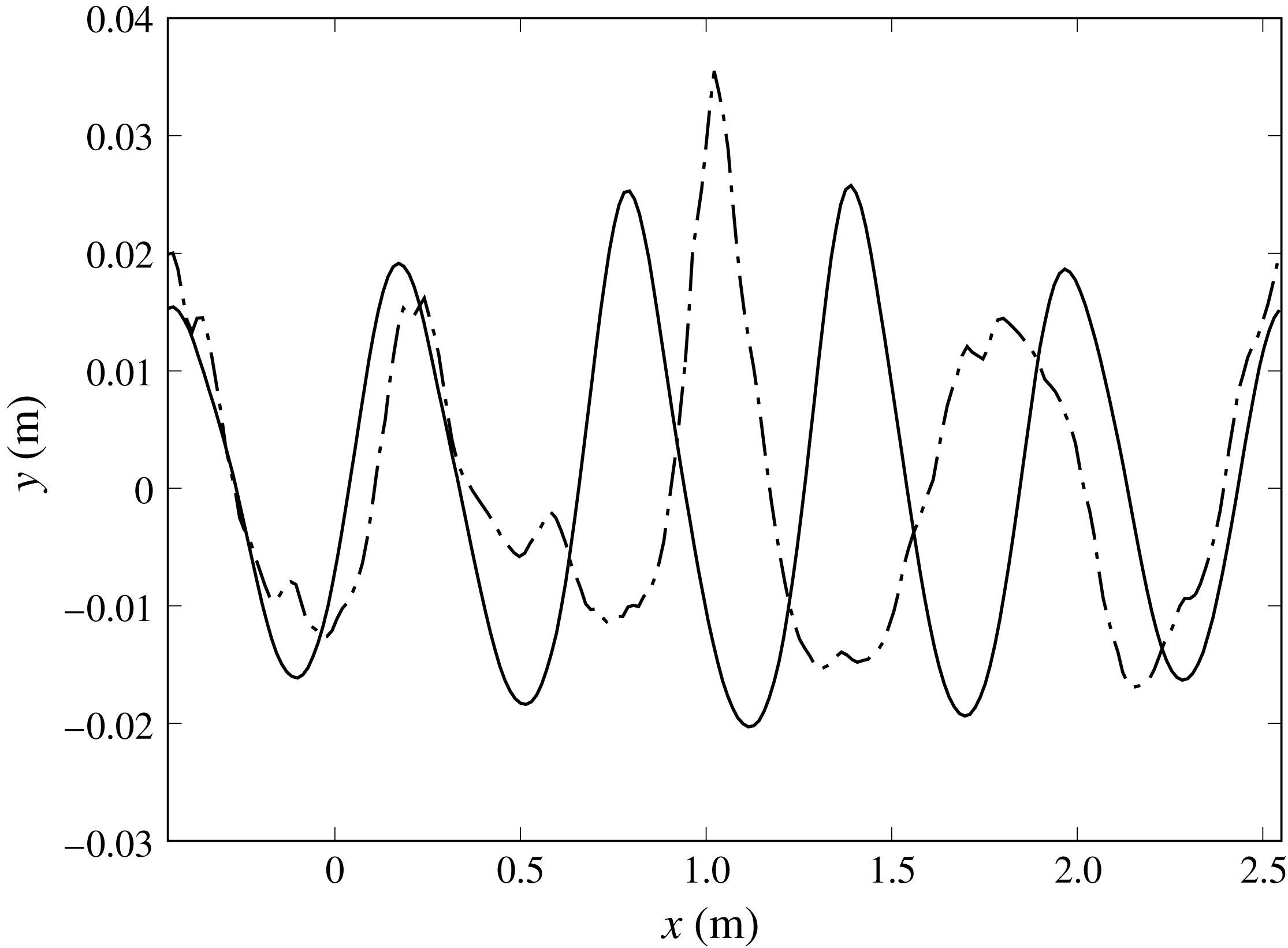
As a consequence of the down-shifting process, the number of waves in the group is reduced from five to four. In the next section it is shown that the phenomenon, which is illustrated in figure 11 and observed experimentally in Tulin & Waseda (Reference Tulin and Waseda1999), significantly contributes to the steepness reduction.

Before closing this section, it is worth remarking that a deeper understanding of the spatial distribution of the frequency components can be achieved by the wavelet transform. By applying such a tool to the free-surface profiles at different stages of the process it is seen that, when the breaking is approached, a very localized high-frequency contribution appears about the crest of the breaking wave, whereas the subharmonic contribution is more uniform in space. These results are in agreement with what discussed in Skandrani, Kharif & Poitevin (Reference Skandrani, Kharif and Poitevin1996). A more extended analysis of the results based on the wavelet transform is still ongoing and will be the subject of future studies.

Figure 11.

Comparison of the free surface at two different times: $t=2$  s (solid line); $t=20$  s (dashed-dot line).

3.3 Free-surface steepness and crest geometry

The crest geometry and its deformation at the onset of the breaking have been widely investigated over the last thirty years. A breaking wave is commonly thought as tilted forward in the direction of the wave propagation with its crest height greater that the trough depth. Motivated by the existence of a limiting wave steepness $\unicode[STIX]{x1D700}_{S}=0.443$ as predicted by the Stokes theory (Perlin et al. Reference Perlin, Choi and Tian2013), several attempts have been made trying to parameterize the crest geometry of the breaking wave and to derive a universal criterion for the prediction of the breaking occurrence. A detailed review of the subject is provided in Perlin et al. (Reference Perlin, Choi and Tian2013) and in the references therein where it is shown that the crest geometry at the onset of the breaking is highly dependent on the way the breaking is achieved and that this makes it difficult to find a universal criterion based on geometric arguments only.

It is worth noticing that the analysis of the crest geometry is generally limited to the first onset of breaking. The use of a two-phase numerical method in simulating the breaking induced by the modulational instability allows us to perform the analysis of the wave geometry not only for the first breaking event but also for the successive events until the end of the process.

In the following the crest geometry is evaluated in terms of the wave steepness expressed as:

(3.1a-c ) $$\begin{eqnarray}S_{dc}=\frac{\unicode[STIX]{x03C0}H_{d}}{L_{dc}},\quad S_{uc}=\frac{\unicode[STIX]{x03C0}H_{u}}{L_{uc}},\quad S_{cs}=\frac{\unicode[STIX]{x03C0}a_{c}}{L_{c}},\end{eqnarray}$$

which denote the down-crossing, up-crossing and crest steepness, respectively. The definitions of the quantities in the equations (3.1) are sketched in figure 12(a). The above parameters are computed for all the waves which are identified in the computational domain. The steepnesses are in descending order. As discussed in the previous section and shown in figure 11, before the breaking five waves are identified in the group whereas four waves remain at the end of the breaking process.

When computing the steepness it is important to distinguish the wave components from the small scale disturbances that are usually associated with the entrained air bubbles and the underwater vorticity structures (see e.g. figure 12 b). For these reasons, when computing the steepness based on either down- or up-crossing criteria, only waves with wavelength greater than half the fundamental wavelength are retained. Similarly, the crest steepness $S_{cs}$ is computed only if the distance between the two zero crossings is greater than one fourth of the fundamental wavelength.

Figure 12.

(a) Sketch of the parameters used to compute the steepness: $c$ is the crest, $z_{u}$ the zero up-cross point, $z_{d}$ the zero down-cross point, $H_{u}$ the wave height using the up-cross definition, $H_{d}$ the wave height based on the down-cross definition, $\unicode[STIX]{x1D706}$ the wavelength, SWL the still water line. (b) Example of small scale structures, mostly vorticity related, which can be interpreted as waves. Note that the horizontal and vertical coordinates are not plotted to the same scale.

In figure 13 the time histories of the steepness of the steepest wave in the domain computed by using the down-crossing and up-crossing definitions are drawn. As already seen in figure 9, the growth of the instability is faster, and thus the breaking starts earlier, for larger initial steepness. Hence, in order to make the comparison easier, the curves are horizontally shifted by the time of breaking onset $t_{b}$ .

As in Deike et al. (Reference Deike, Popinet and Melville2015), the time $t_{b}$ is chosen as the time at which the free surface becomes multi-valued for the first time. This criterion is generally robust for the first breaking event, although, as discussed in the following, it does not allow us to identify the onset of the breaking when it starts as a gentle spilling with single-valued free surface. An example of spilling breaking with single-valued free-surface elevation is shown in figure 2(c) of Diorio et al. (Reference Diorio, Liu and Duncan2009). It is of course more difficult to clearly identify the breaking after the first event as the free surface can become rather complex and multi-valued due to the interaction with bubbles and droplets or with the underwater vorticity. In this case the breaking occurrence can be recognized by the sharp increase in the energy dissipation rate. Unfortunately, it is not so easy to introduce a more quantitative definition.

The results in figure 13 show that, although starting from a different value, both $S_{dc}$ and $S_{uc}$ approach a quite similar behaviour near the breaking point. The curves are characterized by large oscillations with period $2T_{p}$ , which account for the interaction of the wave with the group, and smaller amplitude oscillations with period $T_{p}/2$ which are related to the bound waves. The large amplitude oscillations of the three curves exhibit the same phase and also the growth rates of the peaks are comparable. Nonetheless, the values taken by $S_{dc}$ and $S_{uc}$ at $t=t_{b}$ display large differences in the different cases, with $S_{dc}\in$ (0.35, 0.41) and $S_{uc}\in$ (0.40, 0.48).

During the breaking phase, which lasts approximately $8T_{p}$ , the free surface is not always clear and understandable, mainly because of the chaotic shape of the interface which causes sudden variations of the distance between the zero-crossing points. However, once the breaking phase is over, the steepnesses $S_{dc}$ and $S_{uc}$ continue to oscillate but now they vary in a range, almost independent of time, centred about 0.2 which is far below the pre-breaking value. As already explained, the substantial reduction of the steepness is a consequence of two effects: the reduction of the wave amplitude caused by the energy dissipation and the increase in the wavelength associated with the down-shifting.

Figure 13.

Time evolution of the down-cross (a) and up-cross (b) steepnesses: $\unicode[STIX]{x1D700}_{0}=0.18$ (red solid line); $\unicode[STIX]{x1D700}_{0}=0.20$ (green dotted line); $\unicode[STIX]{x1D700}_{0}=0.22$ (blue dashed-dot line).

A similar analysis can be performed for the crest steepness $S_{cs}$ , which is drawn in figure 14(a). Also in terms of $S_{cs}$ , the solution for the three different cases overlap well before the breaking. However, a much closer agreement is found about the breaking time. From the close-up view provided in figure 14(b) it is seen that the breaking occurs when the crest steepness exceeds 0.71 which is the limiting value of the crest steepness for the Stokes’ wave (Rainey & Longuet-Higgins Reference Rainey and Longuet-Higgins2006). More precisely, the figure shows that in the case $\unicode[STIX]{x1D700}_{0}=0.18$ the parameter exceeds the limiting value already at the previous steepening, approximately two wave periods before. By looking at the free-surface profiles, at the vorticity field below (not shown here) and at the time history of the energy (figure 15 a) it is observed that the wave is already breaking at that time but that the breaking in this case is started by a gentle spilling with single-valued free-surface elevation. In such a condition, the criterion based on the multi-valued free-surface elevation is not able to identify the breaking event, and thus $t_{b}$ is delayed.

The results of figure 14(a) indicate that the breaking induces also a reduction of the crest steepness, but such a reduction is less sharp than that is observed for $S_{dc}$ and $S_{uc}$ in figure 13. For all conditions the crest steepness oscillates and the peak value diminishes in time. However, a better overlapping of the three cases can be noted in comparison to $S_{dc}$ and $S_{uc}$ .

Figure 14.

Time evolution of the crest steepness (a); close-up view about the breaking onset (b): $\unicode[STIX]{x1D700}_{0}=0.18$ (red solid line), $\unicode[STIX]{x1D700}_{0}=0.20$ (green dotted line), $\unicode[STIX]{x1D700}_{0}=0.22$ (blue dashed-dot line), Stokes’ limiting value $S_{cs}=0.72$ (black solid line).

4.1 Breaking parameter, $b$

During each breaking event the energy dissipation is drastically enhanced. Starting from the Phillips’ model, briefly recalled in the Introduction, the energy dissipation is generally expressed as the dissipation rate per unit length of breaking crest:

(4.3) $$\begin{eqnarray}\unicode[STIX]{x1D716}_{l}=b\unicode[STIX]{x1D70C}_{w}c^{5}/g,\end{eqnarray}$$

where $b$ is the breaking parameter. In the original model the parameter $b$ was assumed to be constant but measurements in different conditions showed differences of several orders of magnitude. A much deeper study was performed by Drazen et al. (Reference Drazen, Melville and Lenain2008) who, on the basis of inertial scaling arguments for plunging breaking, proposed for the breaking parameter a dependence $b\sim S^{5/2}$ , $S$ being the wave steepness at the breaking. Romero et al. (Reference Romero, Melville and Kleiss2012) introduced a small change and proposed:

(4.4) $$\begin{eqnarray}b=0.4(S-0.08)^{5/2}\end{eqnarray}$$

motivated by the fact that, according to their measurements, waves with steepnesses below 0.08 do not break and thus the breaking dissipation should vanish.

In order to derive estimates of the coefficient $b$ for the present numerical results, the approach used in Deike et al. (Reference Deike, Popinet and Melville2015) is employed and the energy decay during the breaking is expressed as $E_{w}(t)\sim E_{w0}\exp [-\unicode[STIX]{x1D701}t]$ . With such an assumption, the dissipation rate per unit length $\unicode[STIX]{x1D716}_{l}$ is equal to $E_{w0}\unicode[STIX]{x1D701}$ and the breaking parameter $b$ can be computed as $b=E_{w0}\unicode[STIX]{x1D701}g/(\unicode[STIX]{x1D70C}_{w}c^{5})$ .

The breaking coefficient $b$ can be derived for all the breaking processes. For this purpose, each segment in the energy curves (figure 15 a) corresponding to a breaking event is fitted with an exponential curve to compute the exponent $\unicode[STIX]{x1D701}$ . The velocity $c$ is approximated by the linear phase velocity for gravity waves, as done in Deike et al. (Reference Deike, Popinet and Melville2015).

The estimates of the breaking parameter $b$ for all breaking events are shown in figure 22 where they are compared with the experimental data available in the literature and with the exponential relation. Results are presented in terms of the steepness evaluated both as the sum of the steepness of the initial wave components (figure 22 a), as done in Deike et al. (Reference Deike, Popinet and Melville2015), and as the down-crossing value (3.1) (figure 22 b). The latter is motivated by the fact that in field experiments there is no concept of initial steepness, and thus it can be useful to relate the breaking parameter to the steepness at the onset of the breaking which, instead, can be measured. From figure 22(a) it is seen that the present results agree very well with the data available in the literature and with the exponential dependence suggested in Romero et al. (Reference Romero, Melville and Kleiss2012).

Figure 22.

Breaking parameter $b$ as a function of the steepness: the black line is the relation (4.4); the open red triangles and the solid green triangles are the data in Drazen et al. (Reference Drazen, Melville and Lenain2008) from Scripps Institution of Oceanography (SIO) and Tainan Hydraulics Laboratory (THL) respectively; the open blue diamonds are the data from Melville (Reference Melville1994) at the Massachusetts Institute of Technology; the blue stars are the data for the simulation with $\unicode[STIX]{x1D700}_{0}=0.18$ ; the open magenta boxes are the data from the simulation with $\unicode[STIX]{x1D700}_{0}=0.20$ ; the solid blue boxes are the data from the simulation with $\unicode[STIX]{x1D700}_{0}=0.22$ . For the present numerical data, the steepness is evaluated as the sum of the steepness of the initial wave components in (a) and from the down-crossing criterion at the beginning of the breaking in (b). Figure adapted from Romero et al. (Reference Romero, Melville and Kleiss2012).