2 Equations of motion and parameter regimes

We consider the forced Boussinesq equations in a reference frame rotating about the vertical $\hat{\boldsymbol{z}}$ -direction (Majda Reference Majda2003; Vallis Reference Vallis2006), given by

(2.1) $$\begin{eqnarray}\displaystyle \left.\begin{array}{@{}c@{}}\displaystyle \frac{\text{D}}{\text{D}t}\boldsymbol{u}+f\hat{\boldsymbol{z}}\times \boldsymbol{u}+N\unicode[STIX]{x1D703}\hat{\boldsymbol{z}}+\unicode[STIX]{x1D735}p=\unicode[STIX]{x1D708}\unicode[STIX]{x1D6FB}^{2}\boldsymbol{u}+\boldsymbol{f}_{u},\\ \displaystyle \frac{\text{D}}{\text{D}t}\unicode[STIX]{x1D703}-N(\boldsymbol{u}\boldsymbol{\cdot }\hat{\boldsymbol{z}})=\unicode[STIX]{x1D705}\unicode[STIX]{x1D6FB}^{2}\unicode[STIX]{x1D703}+\boldsymbol{f}_{\unicode[STIX]{x1D703}},\quad \unicode[STIX]{x1D735}\boldsymbol{\cdot }\boldsymbol{u}=0,\end{array}\right\} & & \displaystyle\end{eqnarray}$$

where $\text{D}/\text{D}t=\unicode[STIX]{x2202}/\unicode[STIX]{x2202}t+\boldsymbol{u}\boldsymbol{\cdot }\unicode[STIX]{x1D735}$ is the derivative following fluid particles. The normalized density $\unicode[STIX]{x1D703}(\boldsymbol{x},t)=\sqrt{g/b\unicode[STIX]{x1D70C}_{0}}\unicode[STIX]{x1D70C}(\boldsymbol{x},t)$ has units of velocity, where $g$ is the constant acceleration due to gravity acting in the $-\hat{\boldsymbol{z}}$ direction. The background stratification is linear and aligned with the rotation axis $\hat{\boldsymbol{z}}$ such that the total density is $\unicode[STIX]{x1D70C}_{T}(\boldsymbol{x},t)=\unicode[STIX]{x1D70C}_{0}-bz+\unicode[STIX]{x1D70C}(\boldsymbol{x},t)$ where $\unicode[STIX]{x1D70C}_{0}$ is a constant background density, $b$ is positive for stable stratification and $\unicode[STIX]{x1D70C}$ is the density fluctuation. The Boussinesq approximation assumes $|\unicode[STIX]{x1D70C}|\ll \unicode[STIX]{x1D70C}_{0}$ and $|\unicode[STIX]{x1D70C}|\ll |bz|$ with background in hydrostatic balance $\unicode[STIX]{x1D70C}_{0}g=\unicode[STIX]{x2202}p_{0}/\unicode[STIX]{x2202}z$ . The three-dimensional fluid velocity $\boldsymbol{u}(\boldsymbol{x},t)$ has components ( $u,v,w$ ) and the effective pressure is $p(\boldsymbol{x},t)$ . The Coriolis parameter $f$ is twice the frame rotation rate $\unicode[STIX]{x1D6FA}$ , and the Brunt–Väisälä or buoyancy frequency is $N=(gb/\unicode[STIX]{x1D70C}_{0})^{1/2}$ . Molecular processes are governed by coefficients for kinematic viscosity $\unicode[STIX]{x1D708}$ and mass diffusivity $\unicode[STIX]{x1D705}$ .

Some typical intrinsic scales in such flows may characterize transitions between rotational effects, buoyancy effects and turbulence. The scale at which buoyancy and Coriolis forces balance is the Rossby deformation radius $L_{R}=NH/f$ , which is the horizontal length scale below which stratification effects dominate. In purely stratified flow the outer scale of turbulence above which buoyancy effects dominate is the Ozmidov length scale $L_{O}=\sqrt{\unicode[STIX]{x1D716}/N^{3}}$ . The buoyancy scale $L_{b}=U/N$ down to the Ozmidov scale $L_{O}$ defines a subrange of stratified turbulence. Correspondingly, in purely rotating flow one might define the Zeman length scale $L_{\unicode[STIX]{x1D6FA}}=\sqrt{\unicode[STIX]{x1D716}/f^{3}}$ below which the turbulence isotropizes the flow. In our computations, we aim to resolve the intermediate scales influenced by rotation and stratification, but the Zeman and Kolmogorov scales are under-resolved. This regime also bears analogy to the viscosity-dominated regime in strongly stratified flows with linear PV (Billant & Chomaz Reference Billant and Chomaz2001) wherein viscous effects may influence all scales. In the discussion of the spectra in § 4 below, we will again visit the question of viscosity and resolution. Our focus in this study is not on the small (turbulence) scales but rather on the large and intermediate scales which are more influenced by rotation and stratification.

The Boussinesq equations for rotating, stratified fluids in the inviscid, non-diffusive limit conserve both the total energy, and the potential vorticity following fluid particles (Ertel Reference Ertel1942). Global energy conservation is given by

(2.2) $$\begin{eqnarray}\unicode[STIX]{x2202}_{t}E=\unicode[STIX]{x2202}_{t}\int _{D}E(\boldsymbol{x})\;\,\text{d}\boldsymbol{x}=\unicode[STIX]{x2202}_{t}\int _{D}\frac{1}{2}(\boldsymbol{u}\boldsymbol{\cdot }\boldsymbol{u}+\unicode[STIX]{x1D703}^{2})\;\,\text{d}\boldsymbol{x}=0,\end{eqnarray}$$

where $\int _{D}$ indicates integration over the domain. It may be shown (Kurien, Smith & Wingate Reference Kurien, Smith and Wingate2006; Kurien & Smith Reference Kurien and Smith2014) that this conservation law is independent of $f$ and $N$ . The potential vorticity $q$ on the other hand has explicit dependence on $f$ and $N$ and is defined as

(2.3) $$\begin{eqnarray}q=\unicode[STIX]{x1D74E}_{a}\boldsymbol{\cdot }\unicode[STIX]{x1D735}\unicode[STIX]{x1D70C}_{T}=\unicode[STIX]{x1D74E}\boldsymbol{\cdot }\unicode[STIX]{x1D735}\unicode[STIX]{x1D703}+f\frac{\unicode[STIX]{x2202}\unicode[STIX]{x1D703}}{\unicode[STIX]{x2202}z}-N\unicode[STIX]{x1D714}_{3}+fN,\end{eqnarray}$$

where total vorticity $\unicode[STIX]{x1D74E}_{a}=\unicode[STIX]{x1D74E}+\unicode[STIX]{x1D6FA}\hat{\boldsymbol{z}}$ , the sum of the relative (fluctuating) vorticity $\unicode[STIX]{x1D74E}=\unicode[STIX]{x1D735}\times \boldsymbol{u}$ and the background rotation. The Lagrangian invariance of $q$ , may be written as

(2.4) $$\begin{eqnarray}\frac{\text{D}}{\text{D}t}q=0.\end{eqnarray}$$

Since the constant part $fN$ does not contribute to the dynamics it is normally neglected. PV is by definition, quadratic in the dynamical variables $\boldsymbol{u}$ and $\unicode[STIX]{x1D703}$ . The part of the PV $q_{lin}=f(\unicode[STIX]{x2202}\unicode[STIX]{x1D703}/\unicode[STIX]{x2202}z)-N\unicode[STIX]{x1D714}_{3}$ that is linear (also called the pseudo-potential vorticity) is what is conserved by Charney’s QG model. The reduced models of Bartello (Reference Bartello1995), Babin et al. (Reference Babin, Mahalov, Nicolaenko and Zhou1997), Embid & Majda (Reference Embid and Majda1998), Julien et al. (Reference Julien, Knobloch, Milliff and Werne2006) all conserve the linear part of the PV in their particular parameter regimes as well.

Since the potential vorticity $q$ is a sign indefinite quantity, in practice we use the potential enstrophy as a surrogate to monitor development of $q$ (Kurien & Smith Reference Kurien and Smith2012, Reference Kurien and Smith2014). The total potential enstrophy defined as

(2.5) $$\begin{eqnarray}Q=\frac{1}{2}\int _{D}q^{2}\,\text{d}\boldsymbol{x},\end{eqnarray}$$

is generally quartic. Its quadratic part is

(2.6) $$\begin{eqnarray}Q_{\text{quad}}\equiv \int _{D}q_{lin}^{2}\,\text{d}\boldsymbol{x}=\int _{D}\left(f\frac{\unicode[STIX]{x2202}\unicode[STIX]{x1D703}}{\unicode[STIX]{x2202}z}-N\unicode[STIX]{x1D714}_{3}\right)^{2}\,\text{d}\boldsymbol{x}.\end{eqnarray}$$

The scan of the parameter space in what follows will be accomplished by tracking the potential enstrophy. This approach of defining and tracking the flow parameter regime with reference to linear PV (equivalently, quadratic potential enstrophy) was originally motivated by the existence of quasi-geostrophic and other reduced models in specific limiting cases as discussed in the Introduction. Previous work by one of us has explored exact statistical laws in quadratic potential enstrophy regimes using the fact that $Ro$ and $Fr$ dependencies in the conservation equation are explicit (Kurien et al. Reference Kurien, Smith and Wingate2006). We have also proposed constraints on energy distribution due to simultaneous conservation of potential enstrophy (Kurien, Wingate & Taylor Reference Kurien, Wingate and Taylor2008); and demonstrated joint downscale fluxes of potential enstrophy and energy in a range of linear PV flows (Aluie & Kurien Reference Aluie and Kurien2011). In Kurien & Smith (Reference Kurien and Smith2014) the objective was to quantify structure scales in strongly stratified flows in the linear PV regimes to understand the effect of variable rotation and small aspect ratio. In summary, it is natural and useful to use quadratic potential enstrophy to define our parameter space and to differentiate this work from related work.

The flows of interest for this study are chosen relative to the quadratic potential enstrophy regime. We first choose a value of $f$ such that $Ro=0.005$ which is considered very small, and then vary $N$ so that $Fr\geqslant Ro$ for domain aspect ratio $\unicode[STIX]{x1D6FF}_{d}=1$ . In this parameter variation at fixed $Ro$ , the ratio $N/f$ is varied so that $1/64\leqslant N/f\leqslant 1/4$ . For these values the potential enstrophy is measured and found to be nearly identical with its quadratic component. These data explore unit-aspect-ratio flows for fixed strong rotation and weak to strong stratification. These cases may be thought to be consistent with the parameter regimes for $Ro\rightarrow 0$ and finite $Fr$ for which reduced models were derived by Babin et al. (Reference Babin, Mahalov, Nicolaenko and Zhou1997) (see also Wingate et al. (Reference Wingate, Embid, Holmes-Cerfon and Taylor2011)). Next for the same fixed value of $Ro=0.005$ , the ratio $N/f$ is allowed to assume the same values as for the unit-aspect-ratio case above, but the aspect ratio $\unicode[STIX]{x1D6FF}_{d}$ is varied so that the Burger number $Bu=\unicode[STIX]{x1D6FF}_{d}N/f=1$ . For these simulations too, the potential enstrophy is measured and found to be closely approximated by its quadratic component. This study is closest to the limiting case in Julien et al. (Reference Julien, Knobloch, Milliff and Werne2006) for which reduced models were derived in anisotropic domains for $Ro\rightarrow 0$ with finite stratification.

Departure from the linear PV regimes is investigated by another set of simulations generated by choosing a second value of $f$ such that $Ro=0.02$ and then again varying $N$ and $\unicode[STIX]{x1D6FF}_{d}$ in a manner identical to the above cases. The total potential enstrophy in these cases is found to be different from its quadratic component and hence in its more general quartic form. This is not a controlled departure from linearity, for which we would need a series of simulations with decreasing $Ro$ and growing nonlinearity. Such an effort is beyond the scope of this study. However it is a modest first attempt at understanding how departure from linear PV might affect the scales and structures of such flows.

It must be noted that in all these cases the proximity (or lack thereof) to analytically tractable linear PV regimes must be understood with the caveat that mathematical limiting regimes such as $Ro\rightarrow 0$ , may not be achievable in practical calculations. Furthermore, linear PV may not necessarily imply flows which allow reduced descriptions, even though the converse is true. However given the complexity of the parameter space and the myriad parameter variations available, we choose for this study to make the proximity to controlled and well-defined regimes apparent whenever possible.

3 Numerical simulations, intrinsic scales and some qualitative features

The numerical simulations used to generate the data series were performed using the Sandia-LANL direct numerical simulation (SLDNS) code, and the data were generated on Blue-Gene/Q (Mira, Argonne National Laboratory) using nearly 90 million core hours. Previous work by one of us and collaborators has used the same code as described extensively in Kurien & Taylor (Reference Kurien and Taylor2005), Kurien et al. (Reference Kurien, Wingate and Taylor2008), Aluie & Kurien (Reference Aluie and Kurien2011), Kurien & Smith (Reference Kurien and Smith2012, Reference Kurien and Smith2014). Pseudo-spectral calculations of the Boussinesq equations (2.1) are performed in domains with aspect ratio $\unicode[STIX]{x1D6FF}_{d}=H_{d}/L_{d}\geqslant 1$ , dimensions $L_{d}\times L_{d}\times H_{d}=1\times 1\times \unicode[STIX]{x1D6FF}_{d}$ and $N_{x}\times N_{y}\times N_{z}$ grid points. Although the domain is anisotropic, the computational grid is isotropic, so that $N_{x}=N_{y}=N_{z}/\unicode[STIX]{x1D6FF}_{d}$ . Fourth-order Runge–Kutta time stepping is used, and the inertia–gravity wave frequencies are adequately resolved. The viscosity $\unicode[STIX]{x1D708}$ is chosen dynamically using the scheme of Chasnov (Reference Chasnov1994) which dissipates the energy in the largest shell at each time step. Originally this scheme was formulated to choose a viscous coefficient for hyperviscous modelling of flows and has been used extensively for hyperviscosity powers of 2 and higher (Smith & Waleffe Reference Smith and Waleffe2002). In the present work we use the Chasnov scheme to determine the coefficient for the Navier–Stokes viscous diffusion term, as modelled with the bare Laplacian of the momentum. The motivation for opting for Navier–Stokes diffusion lies in the fact that we are able to attain rather high resolutions for this study, which in principle obviates the need for hyperviscosity and gives a meaningful Reynolds number. We are also aware of the possibility of hyperviscosity introducing spurious effects (Frisch et al. Reference Frisch, Kurien, Pandit, Pauls, Ray, Wirth and Zhu2008). The value of $\unicode[STIX]{x1D708}$ eventually saturates to nearly a constant as the small scales reach statistically steady state. The diffusion coefficient $\unicode[STIX]{x1D705}$ is chosen so that the Prandtl number $Pr=\unicode[STIX]{x1D708}/\unicode[STIX]{x1D705}=1$ .

The Fourier modes are dealiased using the $2/3$ -rule giving an effective small-scale grid of $\unicode[STIX]{x0394}x\times \unicode[STIX]{x0394}y\times \unicode[STIX]{x0394}z=1.5/N_{x}\times 1.5/N_{y}\times 1.5\unicode[STIX]{x1D6FF}_{d}/N_{z}$ . The wavenumber in the horizontal $k_{h}=(k_{x}^{2}+k_{y}^{2})^{1/2}$ has increments $\unicode[STIX]{x0394}k_{h}=2\unicode[STIX]{x03C0}/L_{d}=2\unicode[STIX]{x03C0}$ while the vertical wavenumber has increments $\unicode[STIX]{x0394}k_{z}=2\unicode[STIX]{x03C0}/H_{d}=2\unicode[STIX]{x03C0}/\unicode[STIX]{x1D6FF}_{d}$ . The spherical increment (shell thickness) is defined using the thicker wavenumber increments of the horizontal direction $\unicode[STIX]{x0394}k=\unicode[STIX]{x0394}k_{h}$ . The rate of energy input in all cases is fixed at $\unicode[STIX]{x1D716}_{f}=1$ . The forcing is isotropic, peaked at $k_{f}=4\unicode[STIX]{x0394}k$ , that is, at scales one quarter of the width of the domain. The forcing is divergence free and stochastic with uniformly distributed phase and Gaussian distributed amplitude centred at $k_{f}$ . The energy input is equipartitioned between the three velocity components and the density fluctuations with the result that wave and vortical modes are equally forced at each forced wavenumber. The scheme is identical to that used in Kurien et al. (Reference Kurien, Wingate and Taylor2008) which in turn was motivated by the isotropic forcing implemented in Smith & Waleffe (Reference Smith and Waleffe2002). The characteristic large-scale quantities are defined based on the convention in Babin et al. (Reference Babin, Mahalov, Nicolaenko and Zhou1997) and Smith & Waleffe (Reference Smith and Waleffe2002) for non-unit-aspect-ratio flows: the characteristic velocity is defined as $U=(\unicode[STIX]{x1D716}_{f}/k_{f})^{1/3}$ , the characteristic horizontal scale as $L=2\unicode[STIX]{x03C0}/k_{f}$ and vertical scale as $H=L\unicode[STIX]{x1D6FF}_{d}$ . The non-dimensionalization of the equations of motion then leads to Froude number $Fr=U/(NH)$ , and the Rossby number $Ro=U/(fL)$ . Alternative definitions of $Fr$ based on the horizontal length scale are also common and in our case these would yield smaller $Fr$ and a $Bu$ that is independent of (tall) aspect ratio. To maintain our ability to vary $N/f$ and $\unicode[STIX]{x1D6FF}_{d}$ at a fixed $Bu$ , our definition is appropriate. The Reynolds $Re$ and Prandtl $Pr$ numbers are defined as usual $Re=UL/\unicode[STIX]{x1D708}$ , $Pr=\unicode[STIX]{x1D708}/\unicode[STIX]{x1D705}=1$ .

Table 1.

Simulation parameters of the data sets in the suite of strongly rotating flows. $Ro=0.005$ flows are prefixed by ‘R’; $Ro=0.02$ flows are prefixed by ‘r’. Burger number variation at unit aspect ratio is prefixed by ‘B’; aspect-ratio variation at fixed $Bu=1$ is prefixed by ‘D’.

Table 2.

Summary of naming convention for the ‘R’ (stronger rotation), ‘r’ (weaker rotation), ‘D’ (aspect-ratio varying) and ‘B’ (Burger number varying) simulations. Suffix ‘ $n$ ’ denotes Burger number $1/n$ for the B flows, and domain aspect ratio $n$ for the D flows.

Table 1 lists the external parameters for all the data acquired for this study. The values of $f$ are chosen to fix $Ro=0.005$ and $Ro=0.02$ in the ‘R’ and ‘r’ cases respectively; the values of $N$ are then chosen for $N/f$ values ranging from $1/4$ down to $1/64$ . Burger number variation at unit aspect ratio is prefixed by ‘B’; aspect-ratio variation at fixed $Bu=1$ is prefixed by ‘D’. For the two tallest aspect ratios we lowered the horizontal grid resolution to 512 points in order to manage the very large number of points required in the vertical to retain an isotropic grid, given our computational resources. The Reynolds numbers are calculated based on the viscosity coefficient at the latest time of the simulation after the value has stabilized. The resolution of the Kolmogorov dissipation scale is given by the product $k_{max}\unicode[STIX]{x1D702}$ which is adequate for homogeneous isotropic turbulence (see e.g. Pope Reference Pope2000) but may be marginal for this class of flows in ways that will be discussed in § 4.1. There are therefore four set of variations – the RB-series, rB-series, RD-series and the rD-series. Since the different classes of flows will be referenced repeatedly throughout this paper, the naming convention using these initials has been isolated for easy reference in table 2.

Figure 1.

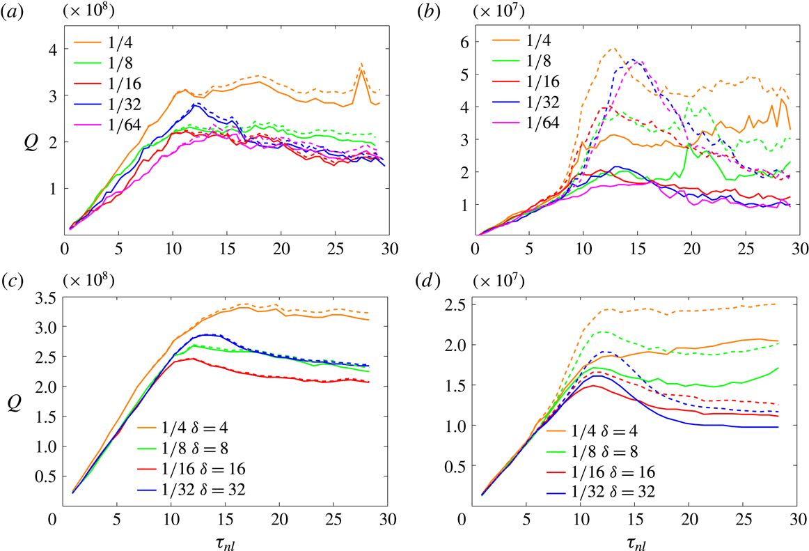
Total potential enstrophy (solid lines) and its quadratic part (dashed lines) as a function of non-dimensional time for various values of $N/f$ for (a) RB-series, (b) rB-series, (c) RD-series and (d) rD-series.

Figure 1 shows the potential enstrophy as a function of non-dimensional time $\unicode[STIX]{x1D70F}_{nl}=t/\unicode[STIX]{x1D70F}$ where the nonlinear time scale $\unicode[STIX]{x1D70F}=(\unicode[STIX]{x1D716}_{f}k_{f}^{2})^{-1/3}$ . These plots demonstrate that the R simulations have quadratic potential enstrophy in the leading order for all values of $N/f$ . In the RB-series, the quadratic potential enstrophy differs from the total by 7 % or less at $N/f=1/4$ . As $N/f$ decreases to $1/64$ , the difference between the two curves is not discernible. The RD series (figure 1 c) shows even closer agreement between the total potential enstrophy and its quadratic part for all values of $N/f$ . Despite some departures, these flows (‘R’-series) will be considered to be the cases defined by leading order quadratic potential enstrophy. By contrast, the r-series shows significant difference between the total and quadratic components of the potential enstrophy, up to 25 % in the tallest-aspect-ratio flow, for example. There are some other qualitative differences. The unit-aspect-ratio RB and rB series show ‘bursts’ of intense potential enstrophy and are in general more noisy than the tall-aspect-ratio D-series, rD and RD, which show relatively smooth development of the potential enstrophy for all $N/f$ . Smoother potential enstrophy for $Bu=1$ cases was also observed for the small-aspect-ratio flows in Kurien & Smith (Reference Kurien and Smith2014) relative to the unit-aspect-ratio flows. Though not shown here, we have checked that the energy in all these cases evolves smoothly. Despite the noisiness (or lack thereof) the important property is the placement of the flows in the regimes of (nearly) quadratic potential enstrophy or far from it.

Figure 2.

Visualization of a $1\times 1$ slice in the $xz$ -plane of $u_{0}$ , the vortical mode of $u$ , for $N/f=1/32$ after $k<5$ modes have been filtered out. (a) RB (b) rB, (c) RD, (d) rD.

Figure 3.

Visualization of a $1\times 1$ slice in the $xz$ -plane of $u_{+}$ , the wave mode of $u$ for $N/f=1/32$ after $k<5$ modes have been filtered out. (a) RB, (b) rB, (c) RD and (d) rD.

Flow visualizations can give a qualitative sense of how structures and scales vary across the range of flows in this suite. For the visualizations shown, the scales $k<5$ have been filtered out so that the forced large scales features do not dominate the images. For clarity of comparison to the unit-aspect-ratio cases, the D-series is shown in a $1\times 1$ subdomain for the $xz$ -plane images. Figure 2 shows vortical-mode visualization of the $u$ -component of the velocity in the $xz$ -plane for all $N/f=1/32$ flows. Clear vertically oriented structures appear in all cases but the structures do not appear identical, indicating the dependence on aspect ratio and on linear versus nonlinear PV regimes. In figure 3 the wave component of the horizontal velocity component $u_{+}$ in the $xz$ -plane shows structures with less extreme vertical orientation than those observed for the vortical mode, suggesting that the wave modes undergo less distortion due to $N/f$ . Again, the structures vary in size and appearance depending on aspect ratio and the respective PV regimes. In the next section we will make more quantitative statements about these dynamical scale and structures that emerge.

4 Analysis and results

For an unbounded or periodic domain, the linear eigenmodes of equation (2.1) are Fourier modes $[\boldsymbol{u}(\boldsymbol{x},t;\boldsymbol{k}),\unicode[STIX]{x1D703}(\boldsymbol{x},t;\boldsymbol{k})]^{\text{T}}=\unicode[STIX]{x1D753}^{m}(\boldsymbol{k})\exp [\text{i}(\boldsymbol{k}\boldsymbol{\cdot }\boldsymbol{x}-\unicode[STIX]{x1D70E}_{m}(\boldsymbol{k})t)]$ with four-component orthogonal basis vectors $\unicode[STIX]{x1D753}^{m}(\boldsymbol{k})$ . There are three types of eigenmodes corresponding to $m=0,\pm 1$ . The $m=0$ modes are usually called vortical modes $\unicode[STIX]{x1D753}^{0}(\boldsymbol{k})$ and have zero frequency $\unicode[STIX]{x1D70E}_{0}(\boldsymbol{k})=0$ . The $m=\pm 1$ modes are two wave modes $\unicode[STIX]{x1D753}^{\pm }(\boldsymbol{k})$ with frequency $\unicode[STIX]{x1D70E}_{\pm }(\boldsymbol{k})$ given by known dispersion relations (see Bartello (Reference Bartello1995), Embid & Majda (Reference Embid and Majda1998), Smith & Waleffe (Reference Smith and Waleffe2002) for explicit expressions for $\unicode[STIX]{x1D753}^{m}(\boldsymbol{k})$ and dispersion relations for $\unicode[STIX]{x1D70E}_{\pm }$ ). The linear eigenmodes serve as a useful orthogonal and complete basis to represent the solution to the full nonlinear equations:

(4.1) $$\begin{eqnarray}[\boldsymbol{u}(\boldsymbol{x},t),\unicode[STIX]{x1D703}(\boldsymbol{x},t)]^{\text{T}}=\mathop{\sum }_{\boldsymbol{k}}\;\mathop{\sum }_{m=0,\pm }b_{m}(\boldsymbol{k},t)\unicode[STIX]{x1D753}^{m}(\boldsymbol{k})\exp [\text{i}(\boldsymbol{k}\boldsymbol{\cdot }\boldsymbol{x}-\unicode[STIX]{x1D70E}_{m}(\boldsymbol{k})t)],\end{eqnarray}$$

where the amplitudes $b_{m}(\boldsymbol{k},t)$ are now the unknowns to be determined (Smith & Waleffe Reference Smith and Waleffe2002; Kurien & Smith Reference Kurien and Smith2012, Reference Kurien and Smith2014). The spectral contributions of the wave and vortical components of the field as a function of wavevector $\boldsymbol{k}$ are respectively:

(4.2) $$\begin{eqnarray}\displaystyle \left.\begin{array}{@{}c@{}}\displaystyle E^{\pm }(\boldsymbol{k},t)=\frac{1}{2}\mathop{\sum }_{m=\pm }|b_{m}(\boldsymbol{k},t)|^{2},\\ \displaystyle E^{0}(\boldsymbol{k},t)=\frac{1}{2}|b_{0}(\boldsymbol{k},t)|^{2}.\end{array}\right\} & & \displaystyle\end{eqnarray}$$

The characteristic scales are computed from the spectra for the wave and vortical modes separately. The utility of this approach was observed in Kurien & Smith (Reference Kurien and Smith2014) where for $Bu\geqslant 1$ and $\unicode[STIX]{x1D6FF}_{d}\leqslant 1$ , markedly different behaviour was observed for the length scales for the vortical versus the wave modes. In addition, since we are interested in the linear PV regimes which are constructed around expansions in the vortical and wave modes, such a distinction is natural. We define the spectral distribution of wave and vortical energy in the horizontal and vertical directions as:

(4.3) $$\begin{eqnarray}\displaystyle E^{\pm [0]}(k_{h},t)=\unicode[STIX]{x0394}k_{z}\unicode[STIX]{x0394}k_{h}\mathop{\sum }_{k_{z}}\mathop{\sum }_{(\unicode[STIX]{x0394}k_{h})_{S}}E^{\pm [0]}(\unicode[STIX]{x1D705}_{h},k_{z}), & & \displaystyle\end{eqnarray}$$

(4.4) $$\begin{eqnarray}\displaystyle E^{\pm [0]}(k_{z},t)=\unicode[STIX]{x0394}k_{h}\unicode[STIX]{x0394}k_{z}\mathop{\sum }_{k_{h}}\mathop{\sum }_{(\unicode[STIX]{x0394}k_{z})_{S}}E^{\pm [0]}(k_{h},\unicode[STIX]{x1D705}_{z}). & & \displaystyle\end{eqnarray}$$

The inner summation in (4.3) indicates summation over wavenumbers $\unicode[STIX]{x1D705}_{h}$ in the annulus of radius $k_{h}$ and thickness $\unicode[STIX]{x0394}k_{h}$ ; the inner summation in (4.4) indicates summation over wavenumbers $\unicode[STIX]{x1D705}_{z}$ on the line fraction centred at $k_{z}$ and width $\unicode[STIX]{x0394}k_{z}$ .

In figures 4–7 we show the vortical and wave energy spectra in the horizontal and vertical directions. In each case only those spectra for the largest and smallest values of $N/f$ in a given data series are shown. All spectra are shown computed at the latest run time of approximately 30 large-eddy turnover times. The wavenumbers $k_{h}$ and $k_{z}$ in the horizontal and vertical directions respectively are given in increments of $2\unicode[STIX]{x03C0}$ for uniformity. Both stronger and weaker rotation cases (R and r) are presented on the same figure for either the B ( $\unicode[STIX]{x1D6FF}_{d}=1$ , variable $Bu$ ) flows or the D (variable $\unicode[STIX]{x1D6FF}_{d}>1$ , fixed $Bu=1$ ) flows. Flows in the R-series are represented by solid lines and those of the r-series by dashed lines. The scaling lines are shown merely as guides to the eye and to bound the behaviour for the reader’s reference.

4.1 Vortical-mode spectra

Figure 4.

Spectra of the vortical-mode energy as a function of horizontal wavenumber $k_{h}$ for two values of $N/f$ as indicated. (a) RB (solid) and rB (dashed), (b) RD (solid) and rD (dashed). Dashed straight lines indicate the minimum and maximum scaling rates for the R flows (solid curves) in each case.

Figure 5.

Spectra of the vortical-mode energy as a function of vertical wavenumber $k_{z}$ for two values of $N/f$ as indicated. (a) RB (solid) and rB (dashed), (b) RD (solid) and rD (dashed). Dashed straight lines indicate the minimum and maximum scaling rates for the R flows (solid curves) in each case.

Figure 6.

Spectra of the wave-mode energy as a function of horizontal wavenumber $k_{h}$ for two values of $N/f$ as indicated. (a) RB (solid) and rB (dashed) and (b) RD (solid) and rD (dashed). Dashed straight lines indicate the maximum and minimum scaling rates for the R flows (solid curves) in each case.

Figure 7.

Spectra of the wave-mode energy as a function of vertical wavenumber $k_{z}$ for two values of $N/f$ as indicated. (a) RB (solid) and rB (dashed) and (b) RD (solid) and rD (dashed). Dashed straight lines indicate the minimum and maximum scaling rates for the R flows (solid curves) in each case.

Figure 4(a,b) shows the distribution of the vortical-mode energy as a function of horizontal wavenumber $k_{h}$ for the lowest and highest values of $N/f$ . The spectral scaling ranges for $k_{h}>10$ or so, and becomes shallower to $k_{h}^{-5/3}$ as $N/f$ decreases. The shallower high-wavenumber scaling at small $N/f$ indicates more energy in the small horizontal scales, corresponding to narrower structures, as the stratification weakens for fixed strong rotation. In the same figure, the dashed lines for the ‘r’ flows lie at or above the corresponding solid lines for the ‘R’ flows, indicating more energy in the horizontal vortical modes of rB compared to RB at all scales. Other features of the spectra such as the dual scaling range for the rB flow at $N/f=1/64$ are outside the scope of this study apart from their potential impact on the centroid (see § 4.3). Such features have been investigated in works such as Rosenberg et al. (Reference Rosenberg, Pouquet, Marino and Minnini2015) and may be related to trade-offs between nonlinear cascade processes and the effect of strong rotation.

The distribution of vortical-mode energy as a function of the vertical wavenumber $k_{z}$ is shown at the largest and smallest values of $N/f$ for RB and rB in figure 5(a) and for RD and rD in figure 5(b). In both figures, the decay rate of energy is far steeper than the corresponding decay rate in the horizontal direction (figure 4 above), consistent with the presence of tall, narrow structures in these flows. For each $N/f$ the r-flow spectrum decays slower than the corresponding R-flow spectrum for both unit (B) and tall (D) aspect-ratio flows indicating more energetic small scales in the r-flows which have smaller rotation rate and hence nonlinear PV.

Adequate resolution becomes a concern in the vertical direction given the quality of the spectra at the high wavenumbers. In figure 5(a), for RB4, $N/f=1/4$ (orange line) spectrum as a function of $k_{z}$ exhibits a slight shallowing and abrupt end at $k_{z}=k_{max}$ instead of the more gradual exponential decay observed in the horizontal spectra. This effect disappears as $N/f$ decreases to $1/64$ (RB64 magenta line). The resolution condition of $k_{max}\unicode[STIX]{x1D702}\geqslant 1.5$ (Pope Reference Pope2000) is satisfied in almost all cases here (see table 1) but that estimate assumes an exponential tail for the spectrum for homogeneous isotropic turbulence (Ishihara et al. Reference Ishihara, Morishita, Yokokawa, Uno and Kaneda2016). We are here in a very different flow regime of highly anisotropic flows, constrained by our requirement of isotropic small-scale grid, isotropic Navier–Stokes dissipation forestalling possible spurious effects of hyperviscosity (Frisch et al. Reference Frisch, Kurien, Pandit, Pauls, Ray, Wirth and Zhu2008), and the maximum resolution we could afford given our computational resources. In flows with Navier–Stokes dissipation, spectra decaying with exponent steeper than $-2$ may not imply maximum dissipation in the smallest scales. Though this issue has not been examined in detail here or elsewhere to the best of our knowledge, the choice of viscosity coefficient based on Chasnov (Reference Chasnov1994) may be less suitable for highly anisotropic flows such as ours in which hyperviscosity is not used to artificially extend scaling ranges and the spectrum in one or more directions is decaying with exponent less than $-2$ . Given these potentially competing factors, the vertical scales for both vortical and wave modes must be assessed with suitable caveats particularly when sampling the small vertical scales at larger $N/f$ , which may be under-resolved. We were able to extend the $N/f=1/4$ simulations by a short period using fixed viscosity of $1.1\times \unicode[STIX]{x1D708}^{\ast }$ where $\unicode[STIX]{x1D708}\ast$ is the stabilized viscosity value at the latest time. The energy spectra resulting from this exercise give us a lower bound on the spectrum at high wavenumbers (not shown) and will be used to assess the error on the vertical scales in the discussions to follow.

4.2 Wave-mode spectra

Figure 6(a) shows the wave energy spectrum as a function of horizontal wavenumber $k_{h}$ for both RB and rB flows for $N/f=1/4$ and $N/f=1/64$ . The spectra in this case have high-wavenumber scaling behaviour ${\sim}k_{h}^{-5/3}$ with a range of steeper scaling near the forcing scale for RB64. Their behaviour is opposite to the vortical modes; the wave-mode energy is marginally higher in the high wavenumbers as $N/f\rightarrow 1$ . Figure 6(b) shows the wave energy spectrum as a function of $k_{h}$ for the RD and rD flows. Again, the wave-mode energy increases as $N/f$ increases. In figure 7 the wave spectra in $k_{z}$ show more pronounced differences as $N/f$ varies, particularly for the R series of flows. As in the case of vertical vortical mode spectra as described above, resolution of the vertical scales might be an issue given the slight shallowing and abrupt end of the spectra as a function of $k_{z}$ for larger $N/f$ .

While the spectral scalings in all cases are shown as guides rather than fits, we can make comparisons with previous work particularly in the $N/f\rightarrow 1$ asymptotic behaviour. In Bartello (Reference Bartello1995) it was shown that for very strongly rotating unit-aspect-ratio flows as $N/f\rightarrow 1$ , the mechanism for downscale cascade of wave energy occurs via a triadic interaction between two wave modes mediated by an unchanging (catalytic) vortical mode, resulting in vortical spectrum scaling as $k^{-3}$ and wave spectrum scaling as $k^{-1}$ in the high wavenumbers. From the tabulated values of the dominant scalings of the R-flows shown in in table 3 we see that for the unit-aspect-ratio B flows the scaling of the vortical mode steepens to $k^{-3.5}$ as $N/f$ increases to $1/4$ ; whereas for the tall-aspect-ratio D flows the scaling of the vortical mode goes to $k^{-4}$ as $N/f$ increases to $1/4$ . This indicates that the approach to asymptotic scaling of the vortical mode occurs more rapidly in unit-aspect-ratio flow than for tall-aspect-ratio flows as $N/f\rightarrow 1$ . For the wave mode, the B-flow spectra hold a steady scaling of ${\sim}k^{-5/3}$ as $N/f$ increases to $1/4$ ; while the D-flows spectral scaling increases from $k^{-3}$ to $k^{-5/3}$ . This shows that in tall-aspect-ratio flows the downscale transfer of wave energy is sharply suppressed as $N/f\rightarrow 0$ (and $\unicode[STIX]{x1D6FF}_{d}$ grows proportionately), much more so than the unit-aspect-ratio flows. As $N/f\rightarrow 1/4$ , the wave spectra of both B and D flows recover similar scaling, indicating that the approach to QG of the wave modes may be comparable.

Qualitatively, the wave-mode spectra contain more energy in the small scales for larger $N/f$ while the opposite was true for the vortical modes. However, both wave and vortical modes express a preference for more energy in the horizontal small scales compared to the vertical small scales, indicating more vertically oriented, columnar flow structures, consistent with distortion due to strong rotation.

Table 3.

Scalings of the horizontal spectra, which are the dominant behaviour, for the vortical and wave modes for the highest and lowest values of $N/f$ in the RB and RD flows.

In the next section we quantify the characteristic scales of all the flows in the suite using centroids and higher-order moments of the spectra and assess the variability of those scales as a function of $N/f$ .

4.3 Spectral moments and length scales

Among the common measures of the characteristic length scales of flows is the integral length scale in physical space, and its equivalent in spectral space (Praud et al. Reference Praud, Fincham and Sommeria2005). The integral length scale is typically associated with the largest energy-containing eddies or structures in the flow. The Taylor microscale is another scale used to characterize flows (Praud et al. Reference Praud, Sommeria and Fincham2006); and direct measurement of vortex thickness has also been used (Hassanzadeh et al. Reference Hassanzadeh, Marcus and Le Gal2012). In Waite & Bartello (Reference Waite and Bartello2006) the second moment of the spectral energy distribution was used to characterize flow scale. In that work it was recognized that the integral length scale may pose some drawbacks due to improper weighting of the large scales (see also Wang & George Reference Wang and George2002) and the choice was made to emphasize the intermediate and small scales more. In Kurien & Smith (Reference Kurien and Smith2014) the first moment, or centroid was used to characterize separately the wave and vortical modes. In the present work we will span a range of moments of the energy distribution as our scale measure. This choice allows us to examine the robustness of any trend that emerges relative to possible large scale effects such as those of the isotropic forced scales or the domain aspect ratio. Especially when considering spectral distributions such as figure 7 which have relatively constant low-wavenumber behaviour (in $N/f$ ), with highly variable steep decay and possible under-resolution observed in the high wavenumbers, it would seem that any dependence on $N/f$ would depend on which scales of the spectrum are being probed. It must be emphasized that whatever the definition and method of scale measurement, comparisons are only justified for the trends as a function of the global parameters, such as the ratio $N/f$ .

The scales $H_{0[\pm ]}^{(n)}$ and $L_{0[\pm ]}^{(n)}$ respectively in the vertical and horizontal directions of the vortical (wave) modes are derived from the $n$ th-order spectral moments as follows:

(4.5) $$\begin{eqnarray}\displaystyle \left.\begin{array}{@{}c@{}}\displaystyle H_{0[\pm ]}^{(n)}=2\unicode[STIX]{x03C0}\left(\frac{\displaystyle \int k_{z}^{n}E^{0[\pm ]}(k_{z})\,\text{d}k_{z}}{\displaystyle \int E^{0[\pm ]}(k_{z})\,\text{d}k_{z}}\right)^{-(1/n)},\\ \displaystyle L_{0[\pm ]}^{(n)}=2\unicode[STIX]{x03C0}\left(\frac{\displaystyle \int k_{h}^{n}E^{0[\pm ]}(k_{h})\,\text{d}k_{h}}{\displaystyle \int E^{0[\pm ]}(k_{h})\,\text{d}k_{h}}\right)^{-(1/n)},\end{array}\right\} & & \displaystyle\end{eqnarray}$$

where the centroid is defined for $n=1$ . To simplify the notation, the superscript $(n)$ in these definitions will be omitted henceforth when the order is made clear by figure captions or other means. In the discussion to follow we will consider moments up to order $n=3$ , with the understanding that increasingly smaller scales are weighed as the order of the moment increases. This approach should give a broader insight into the stability of trends of the scales probed as the smaller-scale effects (higher-order moments) are included. The resulting scale aspect ratios $\unicode[STIX]{x1D6FF}_{0[\pm ]}=H_{0[\pm ]}/L_{0[\pm ]}$ will then be computed and their behaviour as a function of $N/f$ will be assessed across all flows.

In the next section we present the horizontal and vertical scales corresponding to the definition in (4.5) and the spectra in figures 4–7. We show these scales and their aspect ratios as a function of $N/f$ at orders $n=1,2,$ and 3. For the measurements at $n=1$ we will include a data point from an older, lower-resolution simulation for $N/f=1$ ( $Ro=Fr=0.002$ ) at $\unicode[STIX]{x1D6FF}_{d}=1$ , indicated in the plots by a magenta marker. This case was reported in Kurien et al. (Reference Kurien, Wingate and Taylor2008), Kurien & Smith (Reference Kurien and Smith2012, Reference Kurien and Smith2014) and we use it here to indicate the asymptotic behaviour as $N/f\rightarrow 1$ and $\unicode[STIX]{x1D6FF}_{d}\rightarrow 1$ . The forcing for this case was also in the large scales and centred at one quarter the size of the domain. Hyperviscosity was used to artificially extend the scaling range, a standard practice for lower-resolution simulations, in line with other simulations efforts for such flows at the time. The key property that makes this earlier study relevant to the present one is that the former was also in the linear PV regime. This case is in fact the classical Charney QG case, has been studied extensively (Bartello Reference Bartello1995) and is fairly well understood. We show a posteriori that this case lies fairly reliably on the trend lines for the scales in this study. We have checked to make sure that the quantities of interest have converged over the last eddy turnover times in the following sense – while individual length scales are still evolving in time in some cases, the effect across the suite is such that dependence on the global parameter $N/f$ is relatively stable over later times.

Figure 8.

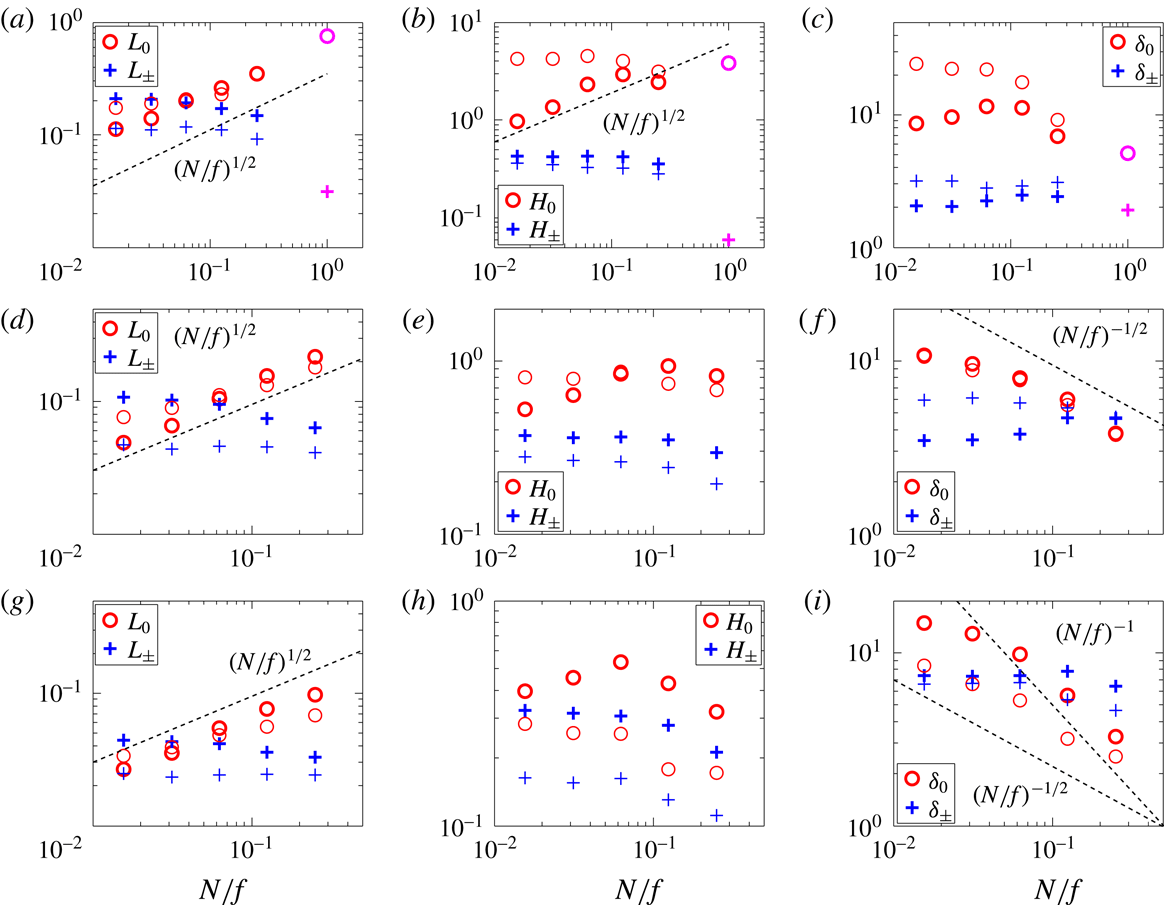
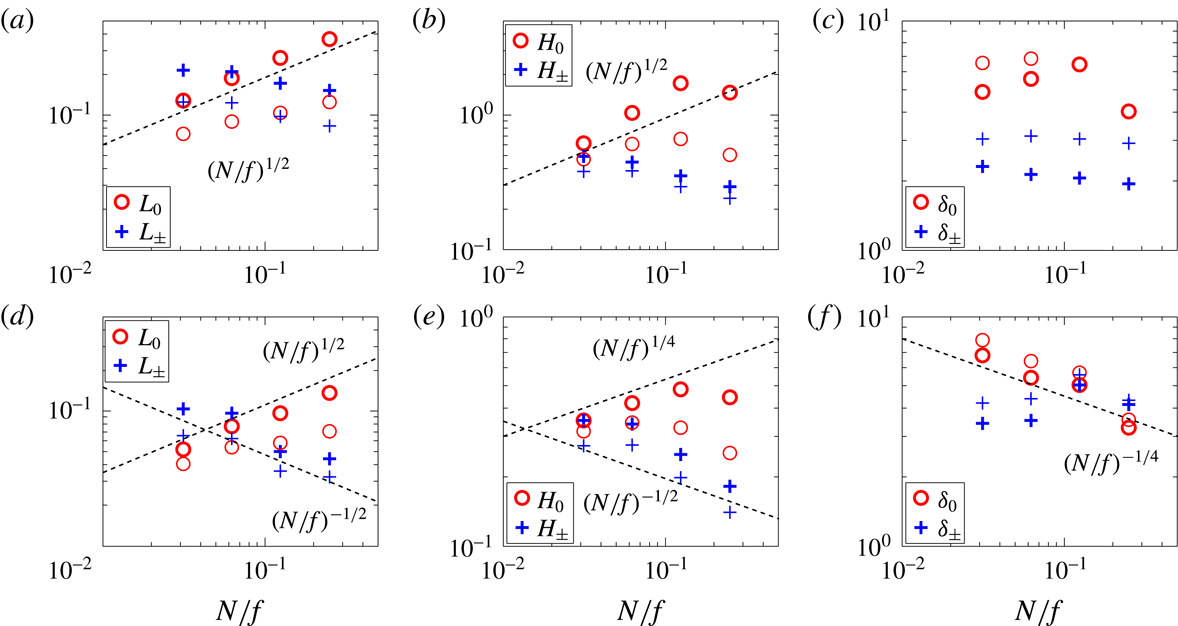
Vortical and wave component length scales for the RB (darker symbols) and rB (lighter symbols) flows as functions of $N/f$ . Column (a,d,g) horizontal scales $L_{0}$ and $L_{\pm }$ . Column (b,e,h) vertical scales $H_{0}$ and $H_{\pm }$ . Column (c,f,i) scale aspect ratios $\unicode[STIX]{x1D6FF}_{0}$ and $\unicode[STIX]{x1D6FF}_{\pm }$ ; $n=1,2,3$ respectively from top to bottom row. The dashed scaling lines are shown as guides to the eye.

4.3.1 Unit-aspect-ratio domains: the RB and rB series

Recall that RB is a Burger number variation study for fixed $Ro=0.005$ with all flows exhibiting nearly quadratic potential enstrophy; and rB is the same study for fixed weaker rotation $Ro=0.02$ for which all flows have quartic potential enstrophy. We first discuss the horizontal and vertical scales as defined by (4.5) for both vortical and wave modes as shown in figure 8. In this figure the order of the moment $n$ used to define the scales increases from 1 to 3 going from the top to the bottom row.

The most stable trend for large to intermediate scales is the $(N/f)^{1/2}$ growth of the horizontal vortical scales $L_{0}^{(n)}$ of the RB flows, which holds up to moment order $n=3$ . This is shown by the darker circles in the first column of figure 8(a,d,g). For $n=1$ , the asymptotic value at $N/f=1$ lies on a trend consistent with the data in this study. The behaviours for the rB (less strongly rotating) flows, shown by the lighter circles in the same plots, show a slightly weaker than $(N/f)^{1/2}$ , but still monotonic, rate of growth. For both RB and rB flows, the magnitude of $L_{0}$ decreases as $n$ increases, consistent with the increased weighting of smaller scales with increase in moment order. As $n$ increases from 1 to 3, the magnitude of these scales decreases by nearly a decade from being of $O(10^{-1})$ to $O(1)$ of the domain width, down to between $O(10^{-2})$ to $O(10^{-1})$ of the domain width.

The vertical vortical scales, shown in the second column of figure 8(b,e,h), show greater variability in $N/f$ as $n$ is increased. The RB flows go from ${\sim}(N/f)^{1/2}$ (b) at $n=1$ to a distinctly non-monotonic scaling (h) in $N/f$ , with growth for $1/64<N/f<1/16$ and decay as $N/f>1/16$ . The smallest of the vertical scales measured occurs at $n=3$ for $N/f=1/4$ (h) at 30 % of the vertical domain size which implies that even at the highest order measured, the vertical characteristic wavenumbers are $k_{z}\leqslant 3$ . We recall that the vertical spectra display some characteristics of under-resolution (see § 4.1 above) in the high vertical wavenumbers $k_{z}>100$ . Therefore, there is some inherent bias in vertical scale measurement that shifts these measurements to smaller scales as the order of the moment $n$ increases. We will reference this bias in our interpretation of the scale aspect ratios below. The rB flows in the same set of plots show little to no dependence of the vertical vortical scale on $N/f$ although their overall vertical scale magnitude does become smaller as $n$ increases, as is to be expected (see figure 5).

The third column of figure 8 shows the aspect ratios computed from the ratios of the vertical and horizontal scales. The RB vortical mode aspect ratio goes from being relative independent of $N/f$ to a decay rate that lies between $(N/f)^{-1}$ and $(N/f)^{-1/2}$ . Since the vertical scales measurement is biased towards the small scales at large $N/f$ the aspect ratios may be under-estimated at large $n$ . Even so, the trend is monotonic decay as $N/f\rightarrow 1$ . For the rB flows the decay occurs at an even slower rate. Both of these aspect-ratio trends arise as $n$ is increased due to the variability the vertical scale $H_{0}$ alone, since the behaviour of the horizontal scale $L_{0}$ is highly stable with respect to $n$ . Compared to the benchmark QG scaling prediction of $(N/f)^{-1}$ for the aspect ratio, we can say that for strongly rotating parameter regimes consistent with (non-QG) reduced models that require linear PV, the vortical-mode aspect ratio displays a somewhat weaker than QG decay rate. This is to be contrasted with the strongly stratified non-QG flows investigated in Kurien & Smith (Reference Kurien and Smith2014) which showed QG scaling of the vortical modes in an identically forced suite of flows. There is thus an asymmetry in the rate of structure growth in $Bu\ll 1$ versus $Bu\gg 1$ flows as a function of $N/f$ at unit aspect ratio even though both extremes can be described by reduced QG-like models requiring linear PV. It is possible, but not completely clear at this level of the analysis, if increasing $n$ further will cause the decay rate of the scale aspect ratio to steepen to the QG value of $(N/f)^{-1}$ . We are unable to reliably increase $n$ further due to concerns of under-resolution at large $N/f$ .

As one scans figure 8 it is immediately apparent that the wave-mode scales, both horizontal $L_{\pm }$ and vertical $H_{\pm }$ (indicated by pluses) are very weakly dependent on $N/f$ . The exception to this is the rapid decay at $n=1$ (a) and (b) from $N/f=1/4$ to $N/f=1$ (the latter data are from the older simulations). With no intermediate data between $N/f=1/4$ and $N/f=1$ it is difficult to extract a trend. In any case, the sharp drop between $N/f=1/4$ and $N/f=1$ separately in the horizontal and vertical scales disappears when considering the wave-mode aspect ratio (c) which shows almost no dependence on $N/f$ . As the moment order $n$ increases, the wave mode aspect ratio increases in magnitude overall, indicating that the smaller scales undergo greater distortion. The rB flows show smaller horizontal and vertical scales than RB flows at all orders $n$ but taller aspect ratios as $n\rightarrow 1$ . This is consistent with greater nonlinearity and hence generation of energetic small scales in these flows, and also suggests that the rB flows undergo greater distortion of the large scales that do the RB flows.

Figure 9.

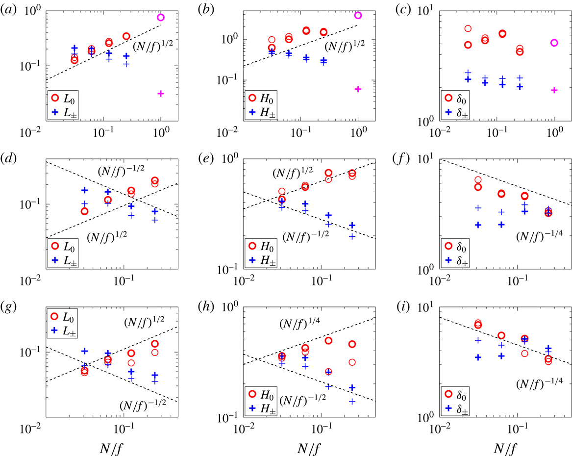
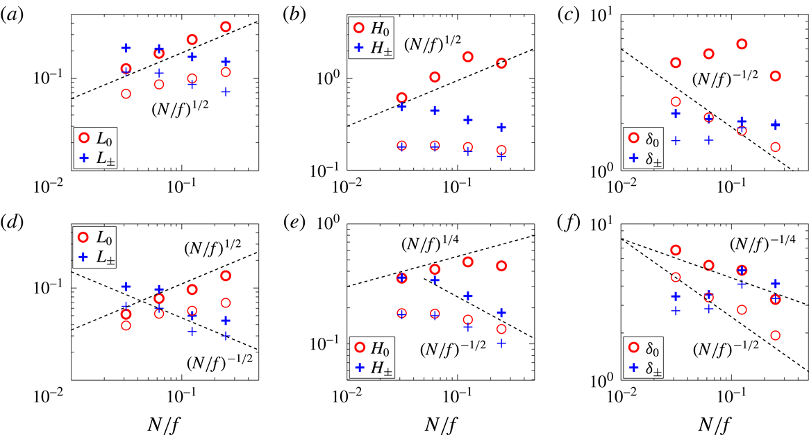
Vortical and wave component length scales for the RD (darker symbols) and rD (lighter symbols) flows as functions of $N/f$ . Column (a,d,g) horizontal scales $L_{0}$ and $L_{\pm }$ . Column (b,e,h) vertical scales $H_{0}$ and $H_{\pm }$ . Column (c,f,i) scale aspect ratios $\unicode[STIX]{x1D6FF}_{0}$ and $\unicode[STIX]{x1D6FF}_{\pm }$ ; $n=1,2,3,$ respectively from top to bottom rows. The dashed scaling lines are shown as guides to the eye.

4.3.2 Tall-aspect-ratio domains: the RD and rD series

These are flows with fixed $Bu=1$ , variable $N/f$ and domain aspect ratio $\unicode[STIX]{x1D6FF}_{d}>1$ ; RD denotes those flows with stronger rotation and hence linear PV, whereas rD denotes those flows with weaker rotation and nonlinear PV. In the first column of figure 9(a,d,g) the vortical-mode horizontal scale $L_{0}^{(n)}$ grows as $(N/f)^{1/2}$ for RD flows for all $n$ ; this is in agreement with the comparable scales discussed above in the unit-aspect-ratio case (figure 8 a,d,g) and is the most stable scaling observed across the entire data suite. The rD flow trend for $L_{0}$ is the same as RD for $n=1,2$ but shows a shallower growth rate for $n=3$ (g). For the same range of $n\leqslant 3$ the vertical vortical scales $H_{0}^{(n)}$ go from close to $(N/f)^{1/2}$ growth (b) to weakly non-monotonic dependence on $N/f$  (h). Consequently the vortical-mode aspect ratio approaches a weak monotonic decay rate of ${\sim}(N/f)^{-1/4}$ as $n$ is increased to 3 (figure 9 i). The weak scaling of the internal aspect ratios of the D flows with respect to $N/f$ is consistent with the steep rate decay of their vertical spectra for wavenumbers larger than the forcing wavenumber as $N/f\rightarrow 0$ . Even with the resolution issues which we have discussed above, the correction to the aspect ratios observed would, if anything, raise their values higher at larger $N/f$ , resulting in even weaker scaling of $\unicode[STIX]{x1D6FF}_{0}$ . Therefore, for this variation of $N/f$ with fixed $Bu=1$ , the tall-aspect-ratio vortical modes do not exhibit QG scaling.

For the wave modes in the D series, also shown in figure 9 (pluses), the horizontal scale $L_{\pm }$ decays weakly as a function of $N/f$ across the RD and Rd flows; this is different from the observation for the B flows (above) which showed no dependence of these scales on $N/f<1/4$ . The asymptotic behaviour as $1/4\leqslant N/f\rightarrow 1$ ( $\unicode[STIX]{x1D6FF}_{d}\rightarrow 1$ ) has a strong decay in $N/f$ (a,b), as for the unit-aspect-ratio case. The vertical scale $H_{\pm }$ in this series also exhibits a weak decay rate in $N/f$ . Consequently, as in the unit-aspect-ratio case, although for different underlying reasons, the wave-mode aspect ratios in the D-series show relative insensitivity to $N/f$ as $n$ is increased (figure 9 c,f,i).

We can now revisit the potential effects of under-resolution of the vertical scales. In both unit and tall-aspect-ratio flows, as discussed above the vertical mode appears under-resolved for large $N/f$ . Using spectra obtained from extending these runs with slightly higher viscosity we obtained a lower bound on the spectrum at high wavenumbers. As a consequence, we find that the value of the vortical-mode aspect ratios may be underestimated by a maximum of 22 % (at $n=3$ ) down to no change at $n=1$ , at the largest value of $N/f=1/4$ . For smaller $N/f$ , the error rapidly diminishes since the under-resolution effect is not nearly as strong (as may be seen in the spectra). On the log–log scale used to discern scaling behaviour with respect to $N/f$ (e.g. figure 8), the correction of ${\sim}20\,\%$ at the highest $N/f$ has a negligible effect on the overall trend in $N/f$ .

Figure 10.

Spectra of the vortical-mode energy as a function of horizontal wavenumber $k_{h}$ for two values of $N/f$ as indicated. (a) RB (solid) and isotropically filtered RB (dashed), (b) RD (solid) and isotropically filtered rD (dashed).

4.3.3 Effect of the large scales: isotropic forcing and anisotropic domains

While the use of larger spectral moment orders places more weighting at the smaller scales as a way to study the robustness of the $N/f$ scaling for the length scales and structure aspect ratios, this approach becomes less effective when contributions to the large scales are substantial. For example, even though the horizontal lengths in RB (figure 8) and RD (figure 9) flows decrease by a factor of 5 as $n$ increases from 1 to 3, the vertical heights remain 50 to 20 % of the horizontal domain size, due to the dominance of the large scales and the rapid spectral decay in spectra as a function of $k_{z}$ (see figures 5 and 7), especially for smaller $N/f$ . Given the peak isotropic forcing scale at 25 % of the horizontal domain size, the large scales, including the forcing scales, could have a strong influence on the structure heights. Nevertheless since the forcing is identical across all the flows independent of $N/f$ , the scaling trends of the length scales in $N/f$ may well result from Boussinesq dynamics, with minimal impact from the forcing. Yet the use of anisotropic domains affects the length scale calculations, as more elongated structures that extend beyond the size of a unit-aspect-ratio domain can now be sampled.

To assess the effects of the large scales, two different filtering schemes are employed to eliminate the spectral contribution at the large scales. The first is an isotropic filter that removes all wavenumbers $k<5$ , which includes the isotropically forced scales. Figure 10 contrasts the original spectra with the isotropically filtered spectra for the vortical-mode energy as a function of $k_{h}$ . Both spectra collapse for $k\geqslant 5$ and only differ for $k<5$ , as expected from the large-scale filtering. Wave mode spectra and spectra as a function of $k_{z}$ behave similarly upon the filtering and are thus not shown. Note that the isotropic filter was also used to render the visualizations in figure 2. The second filter eliminates the spectral contributions anisotropically, by removing both large horizontal modes $k_{h}<5$ and large vertical modes $k_{z}<5$ . Such anisotropic filtering is equivalent to a truncation of the horizontal and vertical spectra shown in §§ 4.1 and 4.2 at $k_{h[z]}=5$ .

Figure 11.

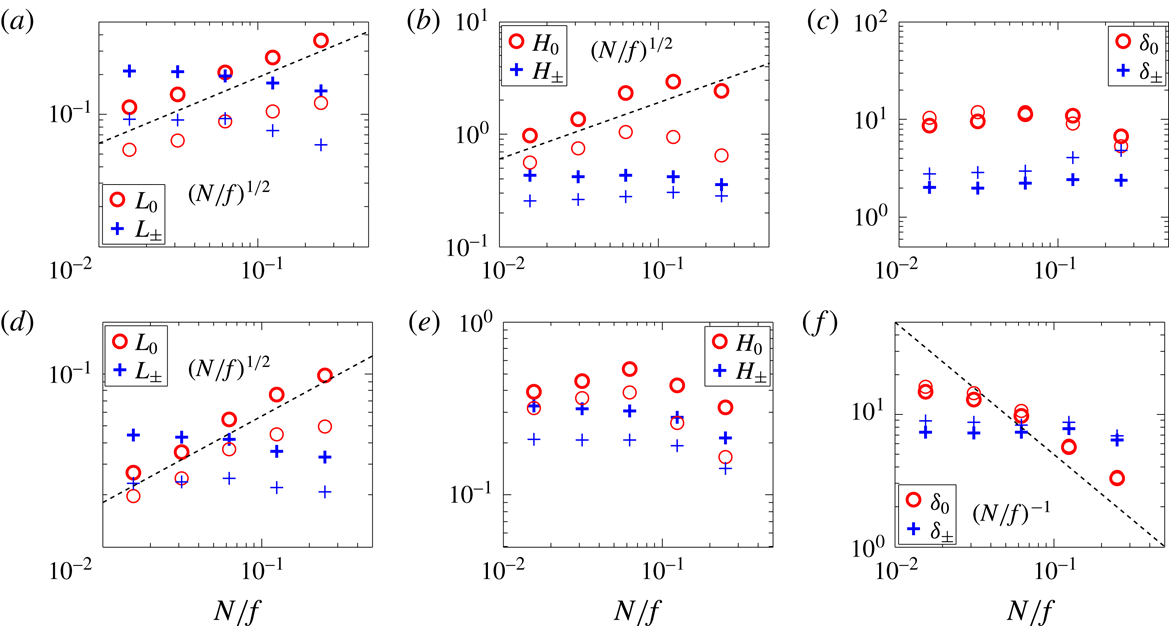
Vortical and wave component length scales for the RB (darker symbols) and isotropically filtered RB (lighter symbols) flows as functions of $N/f$ . Column (a,d) horizontal scales $L_{0}$ and $L_{\pm }$ . Column (b,e) vertical scales $H_{0}$ and $H_{\pm }$ . Column (c,f) scale aspect ratios $\unicode[STIX]{x1D6FF}_{0}$ and $\unicode[STIX]{x1D6FF}_{\pm }$ . $n=1$ and $3$ respectively in top and bottom rows. The dashed scaling lines are shown as guides to the eye.

Figure 12.

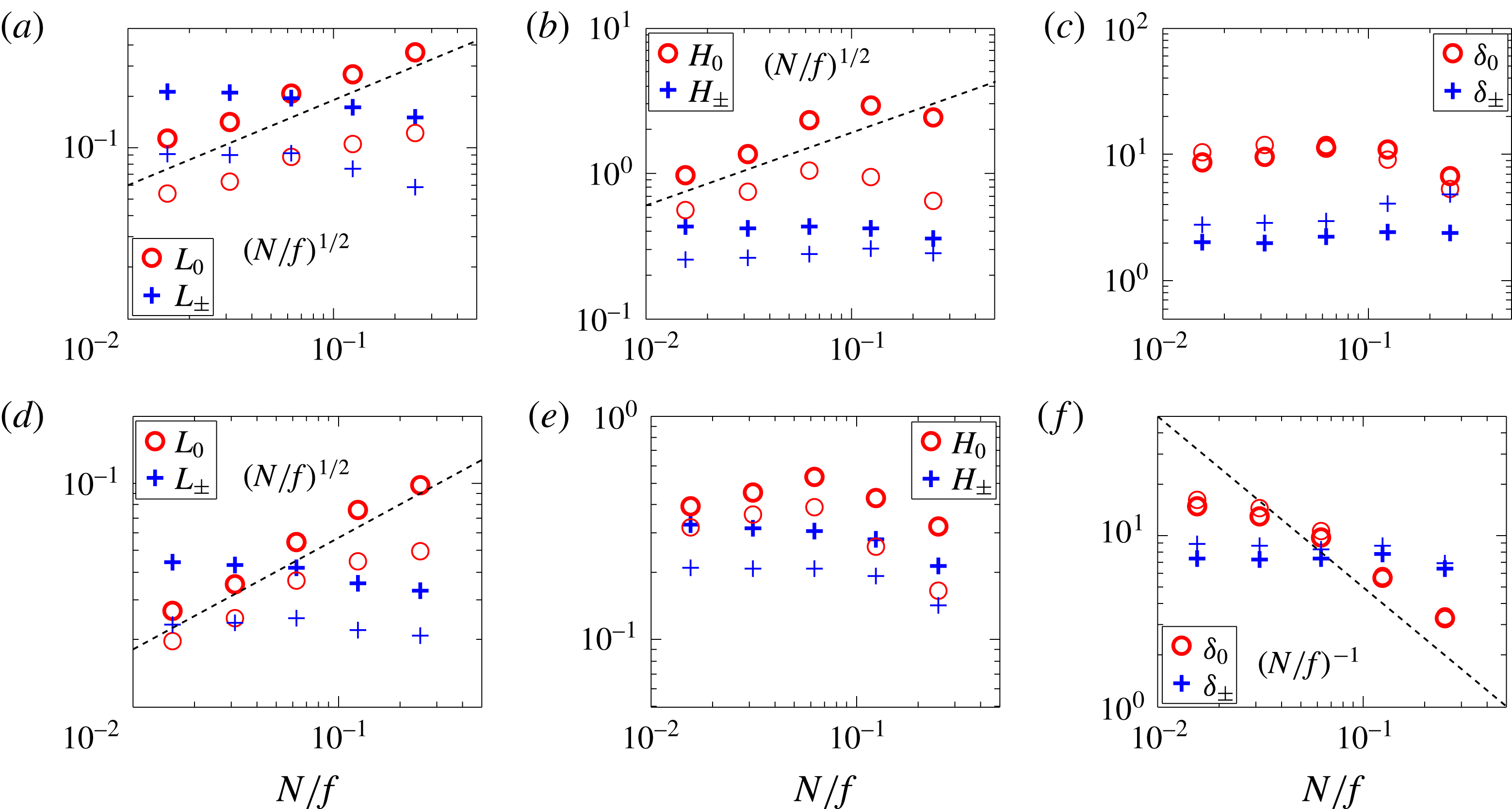
Vortical and wave component length scales for the RD (darker symbols) and isotropically filtered RD (lighter symbols) flows as functions of $N/f$ . Column (a,d) horizontal scales $L_{0}$ and $L_{\pm }$ . Column (b,e) vertical scales $H_{0}$ and $H_{\pm }$ . Column (c,f) scale aspect ratios $\unicode[STIX]{x1D6FF}_{0}$ and $\unicode[STIX]{x1D6FF}_{\pm }$ . $n=1$ and $3$ respectively in top and bottom rows. The dashed scaling lines are shown as guides to the eye.

To illustrate the effects of the large scales, we focus on the RB flows (in unit-aspect-ratio domain) and RD flows (in tall-aspect-ratio domain), and re-compute the length scales using the two filtering schemes. As the spectral contributions to the large scales are filtered, all length scales decrease in magnitude, but the question is whether they do so in a manner that changes their trends as a function of $N/f$ . We mainly compare the trends in $N/f$ scaling with those computed from unfiltered data reported before.

For isotropically filtered data, the scales corresponding to moments of order $n=1$ and 3 are shown in figure 11 for RB flows and figure 12 for RD flows. In the unit-aspect-ratio domains, the vortical-mode aspect ratios $\unicode[STIX]{x1D6FF}_{0}$ from the filtered data (figure 11 c,f) remain essentially identical to those of the unfiltered data. However the horizontal and vertical vortical scales do show some departure from the trends in $N/f$ . Most notably the $L_{0}$ scaling becomes somewhat shallower than $(N/f)^{1/2}$ as $N/f\rightarrow 1$ . These effects may be considered as the corrections to the length scales due to the forced and larger scales, which appear to become stronger as $N/f\rightarrow 1$ . For the wave modes, the aspect ratio $\unicode[STIX]{x1D6FF}_{\pm }$ remains insensitive with $N/f$ upon filtering, yet a larger magnitude of $\unicode[STIX]{x1D6FF}_{\pm }$ is obtained for the filtered case, consistent with the stronger distortion experienced by the smaller scales. The horizontal and vertical scales giving rise to these scale aspect ratios preserve the relative insensitivity to $N/f$ . For the tall-aspect-ratio flows, figure 12 also shows the trend in $N/f$ of the aspect ratio $\unicode[STIX]{x1D6FF}_{0}$ of the vortical modes remains unchanged (figure 12 c,f). The wave modes have larger aspect ratio for the filtered flow, but the shallow trend $~(N/f)^{-1/4}$ is largely unchanged relative to the unfiltered flow. The invariance of the scalings in $N/f$ with and without the forced and larger isotropic scales present suggests that the trends we observe are stable over a wide range in the spectral distributions.

The length scales computed from anisotropically filtered data are shown in figure 13 for the RB flows and figure 14 for the RD flows, along with the corresponding unfiltered data results. In this choice of filtering the extremely large horizontal and vertical structures larger than $20\,\%$ of the horizontal domain size have been removed. For RB and RD flows, the horizontal length $L_{0}$ largely retains scaling of $(N/f)^{1/2}$ while $L_{\pm }$ remains insensitive to $N/f$ . Similar to the isotropically filtered scales shown in figures 11 and 12, $L_{0}$ scaling becomes shallower than $(N/f)^{1/2}$ as $N/f\rightarrow 1/4$ . One notable change is in the vertical heights of $H_{0}$ and $H_{\pm }$ at order $n=1$ : they become roughly constant at approximately 20 % of the horizontal domain size irrespective of $N/f$ for both RB and RD flows, as a result of the anisotropic filtering and the rapid decay of the spectra as a function of $k_{z}$ . Consequently, the vortical-mode aspect ratios in RB and RD flows both show a decay as $(N/f)^{-1/2}$ at order $n=1$ . When $n$ is increased to 3, the vertical height $H_{0}$ decays slightly as $N/f\rightarrow 1/4$ resulting in $\unicode[STIX]{x1D6FF}_{0}\sim (N/f)^{-1}$ in the RB flows, consistent with QG estimates. For the RD flows the $\unicode[STIX]{x1D6FF}_{0}\sim (N/f)^{-1/2}$ remains for $n=3$ . This is steeper than the $(N/f)^{-1/4}$ for the unfiltered flow but not as steep as that achieved for the same measure in the unit-aspect-ratio case. Indeed there is not much difference in the scaling of $\unicode[STIX]{x1D6FF}_{0}$ for RD flows going from $n=1$ to $n=3$ , suggesting that even higher-order moment would not yield different behaviours.

The spectral peak at the forced scales and the rapid decay of the spectra in the vertical direction dominate the characteristic vertical scales in these studies. When these are removed, the largest remaining scales still dominate at low-order $n$ and therefore one needs to probe higher-order moments to obtain non-trivial scalings. It is notable that the decay rate of vortical scale aspect ratio steepens as a function of $N/f$ as one probes scales away from the largest and forced scales. While these scalings may not have converged with respect to moment order, the Boussinesq dynamics is arguably the dominant cause for the scaling that emerges at higher-order moments after filtering.

Figure 13.

Vortical and wave component length scales for the RB (darker symbols) and anisotropically filtered RB (lighter symbols) flows as functions of $N/f$ . Column (a,d) horizontal scales $L_{0}$ and $L_{\pm }$ . Column (b,e) vertical scales $H_{0}$ and $H_{\pm }$ . Column (c,f) scale aspect ratios $\unicode[STIX]{x1D6FF}_{0}$ and $\unicode[STIX]{x1D6FF}_{\pm }$ . $n=1$ and $3$ respectively in top and bottom rows. The dashed scaling lines are shown as guides to the eye.

Figure 14.

Vortical and wave component length scales for the RD (darker symbols) and anisotropically filtered RD (lighter symbols) flows as functions of $N/f$ . Column (a,d) horizontal scales $L_{0}$ and $L_{\pm }$ . Column (b,e) vertical scales $H_{0}$ and $H_{\pm }$ . Column (c,f) scale aspect ratios $\unicode[STIX]{x1D6FF}_{0}$ and $\unicode[STIX]{x1D6FF}_{\pm }$ . $n=1$ and $3$ respectively in top and bottom rows. The dashed scaling lines are shown as guides to the eye.

Figure 15.

Kinetic, potential and total energy scale aspect ratios $\unicode[STIX]{x1D6FF}_{K},\unicode[STIX]{x1D6FF}_{P}$ and $\unicode[STIX]{x1D6FF}_{E}$ for the RB flows. Panels from left to right are computed at $n=1$ , 2 and 3 respectively. The $Bu=1$ unit-aspect-ratio case is shown in magenta for $n=1$ .

4.3.4 Mixed scaling of kinetic, potential and total energy spectral moments

In Kurien & Smith (Reference Kurien and Smith2014) it was proposed that quantities that have mixed dependence on the wave and vortical modes, such as, for example, a single component of velocity, vertical vorticity, the kinetic energy or even the total energy, may express length scales which have some non-trivial combination of wave- and vortical-mode scalings. This fact is relevant when comparing with other length scale measurements, particularly those that arise from experiments (Praud et al. Reference Praud, Sommeria and Fincham2006; Aubert et al. Reference Aubert, Le Bars, Le Gal and Marcus2012) which do not typically project their data onto the linear eigenmodes.

We calculate the scale aspect ratios $\unicode[STIX]{x1D6FF}_{K}^{(n)},\unicode[STIX]{x1D6FF}_{P}^{(n)},\unicode[STIX]{x1D6FF}_{E}^{(n)}$ from the kinetic, potential and total energy spectra using definitions analogous to (4.5). Figure 15 shows these quantities for the unit-aspect-ratio RB flows. The scale aspect ratios computed from total energy spectra display weaker dependence on $N/f$ than does the aspect ratio computed from the potential energy for $n=1$ . This is consistent with the fact that although the vortical-mode aspect ratios approach a decay rate of $(N/f)^{-1/2}$ , the wave modes remain insensitive to $N/f$ (see figure 9 c,f,i). The kinetic energy based aspect ratio $\unicode[STIX]{x1D6FF}_{K}$ , which has vortical and wave contributions from the horizontal velocity and a purely wave contribution from the vertical velocity seems to show independence to $N/f$ similar to wave modes, while the potential energy based aspect ratio $\unicode[STIX]{x1D6FF}_{P}$ seems to exhibit something like a decay with respect to $N/f$ , similar to vortical modes. Thus, the scales computed based on quantities that mix the eigenmodes will display mixed scaling. This is particularly relevant when seeking to benchmark against the QG scaling of $f/N$ . It appears from our study above that the vortical mode aspect ratios can approach the monotonic decay and even QG scaling of $(N/f)^{-1}$ for scales far from the forced scales, while the wave modes remain relatively insensitive to $N/f$ . This behaviour is obscured when mixed quantities are considered.

5 Discussion and conclusions

We have presented measurements of the characteristic scales that emerge in numerical simulations of the Boussinesq equations for isotropically forced strongly rotating flows with fixed high Coriolis frequency $f$ and variable moderate to weak buoyancy frequency $N$ in periodic domains with aspect ratio $\unicode[STIX]{x1D6FF}_{d}\geqslant 1$ . We have performed a systematic study in the parameter space of $N/f$ , $\unicode[STIX]{x1D6FF}_{d}$ and $Bu=Ro/Fr=\unicode[STIX]{x1D6FF}_{d}N/f$ in order to disentangle as much as possible the effects of each on the development of characteristic scales. Since the parameters are related via $Bu$ we opted for a partial exploration of the parameter space by fixing $\unicode[STIX]{x1D6FF}_{d}=1$ for a variable $Bu<1$ study, and fixing $Bu=1$ for a variable $\unicode[STIX]{x1D6FF}_{d}>1$ aspect-ratio study, both choices in deference to known asymptotic theories. In an attempt to connect to the quasi-geostrophic and other reduced model parameter regimes, one series of flows, the R-series, with $Ro=0.005$ has linear potential vorticity (quadratic potential enstrophy) and the other, the r-series, with $Ro=0.02$ has quadratic potential vorticity (quartic potential enstrophy). The particular values of $Ro$ in these cases are not as important as the fact that they place the flows in the desired regime for the available grid resolution.

We quantify the characteristic scales that emerge in our suite of flows using the weighted moments of the spectra of the vortical and wave modes in both horizontal and vertical directions. The separation of wave and vortical-mode scales is an important feature of our study since these eigenmodes exhibit different sensitivities to the ratio $N/f$ . Using the definitions in (4.5) we measure the following: vortical (wave) horizontal length scales $L_{0[\pm ]}$ , vortical (wave) vertical length scales $H_{0[\pm ]}$ and their aspect ratios $\unicode[STIX]{x1D6FF}_{0[\pm ]}=L_{0[\pm ]}/H_{0[\pm ]}$ . The variability of these quantities is explored as a function of $N/f$ . Higher-order moments increasingly weigh the higher wavenumbers (smaller scales) and therefore help to evaluate the robustness of the scaling behaviours observed.

We also assess the effect of the large scales explicitly by using two different filtering schemes – the first is an isotropic filter that removes all modes $k<5$ , which includes the isotropically forced modes, and the second is an anisotropic filter that removes all $k_{h}<5$ and $k_{z}<5$ , that is, the widest pancake and tallest columnar structures. In combination with scale measurement at higher-order $n$ the filtering strategy allows better access to the intermediate and smaller scales of the flow, which are unbiased by forcing and other large-scale effects.

The benchmark theoretical result against which we evaluate our scale measurements is the quasi-geostrophic (QG) estimate that the aspect ratio of vortical-mode structures varies as $(N/f)^{-1}$ (McWilliams Reference McWilliams1985). A feature of all the flows in this study is that they lie outside of the parameter range in which Charney’s QG equations hold. Given the results in Kurien & Smith (Reference Kurien and Smith2014) which recovered QG scaling of the vortical-mode aspect ratio in strongly stratified regimes with $N/f\gg 1$ , it is of interest then to assess how, if at all, the systematic scaling of structure aspect ratio extends into the strongly rotating regime.

This investigation at the outset raised the question of whether, and to what extent, the QG-based scaling estimate of scale aspect ratio ${\sim}(N/f)^{-1}$ might hold for Boussinesq flows that are theoretically far from QG but in regimes with linear PV. It is found that the aspect ratio $\unicode[STIX]{x1D6FF}_{0}$ of the vortical mode shows monotonic decay for $n>1$ in both unit and tall-aspect-ratio domains. The decay rate steepens for larger $n$ , from $(N/f)^{-1/2}$ to slightly shallower than $(N/f)^{-1}$ for $n=3$ in the unit-aspect-ratio flows, and towards $(N/f)^{-1/4}$ at $n=3$ in the tall-aspect-ratio flows. While isotropic filtering leaves $\unicode[STIX]{x1D6FF}_{0}$ largely unaffected, anisotropic filtering leads to slightly steeper decay rate for both unit and tall-aspect-ratio flows. A plausible interpretation of our results is that unit-aspect-ratio domains permit QG scaling as an underlying feature of the intermediate scales, that is, downscale from the forcing, for the vortical modes alone. The tall-aspect-ratio domains do not display such a behaviour for the same range of $N/f$ , indicating a fundamental difference between flows with $N/f<1$ , that arises due to domain aspect ratio.

These results may be contrasted with studies of stratification-dominated flows with $N/f\gg 1$ for which the aspect ratio of the vortical modes decayed as $(N/f)^{-1}$ with a low-order measurement at $n=1$ (Kurien & Smith Reference Kurien and Smith2014). This difference between $N/f>1$ and $N/f<1$ structure scaling is consistent with the conclusion of Sukhatme & Smith (Reference Sukhatme and Smith2008) which noted an asymmetry in the transition in Boussinesq flows from $N/f\leqslant 1$ to $N/f\geqslant 1$ , both of which are formally consistent with QG. In the former (slightly rotation dominated) the wave energy grows to dominate the overall energy and the QG vortical component has an energetically smaller role, while in the latter (slightly stratification dominated), the wave energy saturates and the QG signature is dominant.

Apart from our study of the scaling of $\unicode[STIX]{x1D6FF}_{0}$ , we have also observed a stable scaling with respect to $N/f$ for the vortical mode horizontal length scale $L_{0}\sim (N/f)^{1/2}$ . This scaling appears to hold irrespective of domain aspect ratio, or the order (up to $n=3$ ) of the spectral moment from which the scale is derived. There is a slight deviation from this scaling for the r-series compared to the R-series, indicating that linear PV may be required for this scaling behaviour. When the largest scales are removed either isotropically (as the forced scales) or anisotropically (by removing the tallest and widest modes), the result is monotonic but somewhat slower growth than $(N/f)^{1/2}$ as $N/f\rightarrow 1$ . We interpret this to mean that as $N/f\rightarrow 0$ the $L_{0}\sim (N/f)^{1/2}$ scaling emerges as a stable feature of non-QG flows with $N/f\ll 1$ . This result is not one that we have a predictive model for at present, but it appears to be robust enough to hold over a substantial range of scales and it deserves some more rigorous treatment in the future.

The differences in scaling for the r-flows (nonlinear PV) occur most notably for the characteristic scale height in unit-aspect-ratio flow. In these rB cases, the $H_{0}$ go from being larger than those for RB at $n=1$ to being smaller than those for RB at $n=3$ . However, the dependence on $N/f$ is fairly uniform, that is, the r-series is not as sensitive to $N/f$ as is the R-series. This results in a weaker decay of $\unicode[STIX]{x1D6FF}_{0}$ for rB than for RB. The scalings of the rD flows are comparable to those of the RD flows, both of which are very weakly dependent on $N/f$ . Nonlinear PV thus appears to have a greater impact on structure scales in the unit-aspect-ratio domains than in the tall-aspect-ratio domains. In the latter, the domain shape is the dominant effect.

This study was done with the best resolution that we could manage given our computational resources. It could well be that if the tallest-aspect-ratio cases were to be performed with greater resolution, some more refined estimates of the scales would arise. Our choice to fix $Bu=1$ while varying $N/f$ and $\unicode[STIX]{x1D6FF}_{d}$ is also an important factor in the outcomes observed. A different choice of (say) fixed $Bu<1$ and varying $N/f$ accordingly would allow for the exploration of the scalings observed on $Bu$ . At this level of the discussion, we can say that tall-aspect-ratio strongly rotating flows display quantitatively different scale development than unit-aspect-ratio flows for the same variation in $N/f$ . It is suggested, based on these results, that a different type of mechanism in terms of resonances or near resonances exists for reduced models in these tall-aspect-ratio parameter ranges. It is hoped that the type of analysis presented here motivates further fundamental studies in the tall-aspect-ratio and strongly rotating flow regimes.