2.1. Set-up and main features of RF-generated plasmas

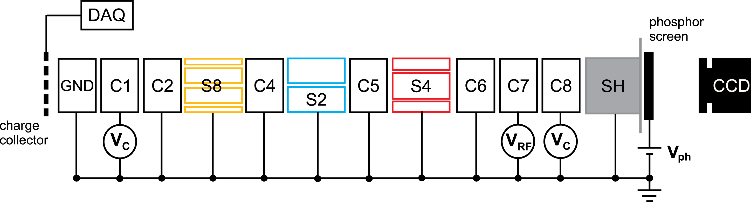
The experiments presented here were performed in the ELTRAP (ELectron TRAP) Penning–Malmberg device, a machine where a vacuum vessel kept in the UHV regime (typically $10^{-8}{-}10^{-9}~\text{mbar}$ ) houses a stack of 12 cylindrical electrodes (sketched in figure 1) with a maximum trapping length $L_{trap}$ of about 1 m and a 45 mm radius $R_{W}$ . While the two outermost electrodes are permanently grounded to ensure a well-defined potential outside the trapping region, any pair of inner electrodes can be used as endcaps to create a positive or negative well with a depth $V_{C}\leqslant 100~\text{V}$ . The vessel is surrounded by a solenoid providing a highly homogeneous axial magnetic field $B\leqslant 0.2~\text{T}$ . In these conditions, typical low-temperature electron plasmas are highly magnetized, with a cyclotron frequency ${\it\nu}_{c}=eB/2{\rm\pi}m$ (where $e$ and $m$ are the electron charge and mass) in the GHz range and a cyclotron radius orders of magnitude smaller than $R_{W}$ . Other typical frequencies, characteristic of the transverse $\boldsymbol{E}\times \boldsymbol{B}$ drift, are the plasma rotation frequency ${\it\nu}_{r}$ and the frequencies of diocotron (azimuthal) $l$ -modes ${\it\nu}_{l}$ that lie in the 10–100 kHz range. The axial bounce frequency ${\it\nu}_{z}$ is about 0.1–1 MHz for temperatures of few eV. These motions are therefore decoupled in the non-collisional regime, yet collisions may become relevant in long-time experiments, as the electron–electron collision frequencies have values around some 100 Hz and electron–neutral collision frequencies lie in the 1–10 Hz range. Non-destructive diagnosis of the plasma transverse motion is possible by monitoring the current induced by the plasma itself on azimuthally split electrodes S2, S4, S8 (segmented into two, four and eight equal patches, respectively). Grounding one of the endcaps allows the plasma to flow out and to be intercepted either by a collector plate or by a phosphor screen biased at a positive voltage $V_{ph}\sim 5{-}15~\text{kV}$ , respectively, so that the total charge or the axially-integrated electron distribution is acquired.

Figure 1.

Sketch of the trap electrode arrangement. Outer electrodes GND and SH are permanently grounded. Any pair of two electrodes can be set to a confinement potential $V_{C}$ to be used as endcaps while another one is employed as excitation antenna with an oscillating voltage signal $V_{RF}$ . Diagnostic tools are also sketched: a charge collector connected to a high-impedance digital oscilloscope and a phosphor screen set to a potential $V_{ph}=5{-}15~\text{kV}$ , whose image is recorded by a CCD camera.

Contrary to customary Penning traps exploiting electron sources like thermocathodes or photocathodes, the RF production mechanism discussed here is ‘sourceless’ in that it uses no additional physical apparatus. The procedure starts with a confinement configuration where two endcaps are biased to a negative potential $V_{C}=80{-}100~\text{V}$ and all other electrodes are grounded apart from a chosen electrode within the confinement region, set at a sinusoidally varying voltage $V_{RF}\sin (2{\rm\pi}{\it\nu}_{RF}t)$ with a typical amplitude $V_{RF}=1{-}5~\text{V}$ and a frequency ${\it\nu}_{RF}$ ranging from 1 to some 10 MHz. An electron plasma can be detected in times of the order of some 100 ms and a stable distribution characterized by a dynamical equilibrium between continuous formation and losses is reached after some seconds. In particular, axial losses of electrons with an energy overcoming the trapping barrier can be detected in the form of continuous currents up to some nA flowing onto the collector. Even if ions are not effectively confined, ionization must also produce a continuous flux of molecular ions through the trapping volume. So far, we have not been able to obtain any direct information on the ion plasma component, whose measurement presents technical difficulties. In other experiments ad hoc diagnostic techniques have been developed to this end (Kabantsev & Driscoll Reference Kabantsev and Driscoll2004) which are not easily applied in our system.

A qualitative explanation of the plasma generation phenomenon can be given on the basis of simple arguments. Given the axisymmetric geometry of the confinement and excitation electrodes and the frequency range of the RF drive, free electrons in the background gas may be heated, predominantly in the axial direction, which in turn may lead to ionization of the residual gas when the electrons reach sufficient kinetic energy, following a mechanism of stochastic nature (Lichtenberg & Lieberman Reference Lichtenberg and Lieberman1983). An interpretation of heating and ionization phenomena in terms of stochastic heating due to oscillating electric fields has been proposed in the past, e.g. in the context of RF discharges at higher pressures ( $10^{-3}{-}1~\text{mbar}$ ) where extended experimental results as well as theoretical models have been obtained (Lieberman & Godyak Reference Lieberman and Godyak1998; Wang, Lichtenberg & Cohen Reference Wang, Lichtenberg and Cohen2012). In our experimental observations typical plasma formation times (hundreds of ms) match the aforementioned collisional times and the RF drive frequencies agree with the bounce frequencies of electrons with axial kinetic energy of few to tens of eV, thus qualitatively confirming this interpretation. Further details can be found in Paroli et al. (Reference Paroli, De Luca, Maero, Pozzoli and Romé2010b ) and Romé et al. (Reference Romé, Chen, Maero, Paroli and Pozzoli2015). Linear and nonlinear resonances of the RF field with the axial particle motion or with longitudinal collective modes can also contribute to the heating effect.

Over the course of many experiments we observed that additional ionization sources, e.g. UV rays or static high voltages (HV), may help to initiate the discharge. This is particularly helpful at the beginning of the experiment, i.e. UV or HV can be used as an initial trigger when starting from scratch and then switched off so that the subsequent generation of further electron samples after ejection of the previous, early plasmas can continue without additional help. Please note that in order to use the optical diagnostics we necessarily set the phosphor screen to a voltage in the kV range. In order to avoid possible distortion in the results, the phosphor voltage has been permanently switched on at a value of 8 kV for all experiments presented in the following. Nevertheless it is important to remark that many experiments have been performed where we could attain repeated ‘create–hold and measure–dump’ sequences of RF-generated plasmas without the need for UV or HV; therefore we can exclude the possibility that these represent the direct origin of the observed phenomena.

Plasmas generated by means of this procedure reach a total charge up to about 1 nC and particle densities in the range $10^{6}{-}10^{7}~\text{cm}^{-3}$ . The plasma is most frequently produced close to the electrode surface in the early formation stage over typical time periods in the 100 ms range. The charge progressively builds up and may reach a status where it covers the whole trap cross-section. As we will see in the following, in general the density is relatively low with respect to specific events that we could observe, namely the formation of columns with a narrower mean radius $R_{p}$ or the transition from a diffuse plasma to a denser and smaller cross-section. These electron plasmas can have a radius as small as $R_{p}/R_{W}\leqslant 0.1$ and yield particle densities above $10^{7}~\text{cm}^{-3}$ , and we have previously exploited this phenomenon mainly as a substitute for a more conventional electron plasma source, as it allows us to ‘prepare’ an electron column for the following observation stage where the excitation drive is switched off and the plasma is left free to evolve. In such cases the RF generation phenomenon is used as a tool and we empirically adjust the control parameters in order to achieve a plasma with the desired features to perform a subsequent experiment.

The narrow-radius plasmas exhibit further interesting features. They are often produced at a radial offset with respect to the magnetic axis and hence exhibit an $l=1$ diocotron mode (i.e. a drift around the magnetic axis). Experiments on quiescent plasma columns have shown that the $l=1$ mode is unstable in the presence of various sources of dissipation, including the presence of positive ions (Fajans Reference Fajans1993). Continuous ionization implies the presence of ionic species in the trap during the RF plasma generation; we found that as long as the RF drive is on, the mode is stable or presents a slow amplitude and frequency modulation (Paroli et al. Reference Paroli, Maero, Pozzoli and Romé2014).

All experiments presented in the following were performed according to a common routine, namely the repetition of the ‘create–hold–dump’ loop and the acquisition of the image formed on the phosphor screen at the release of the plasma and recorded by a charge-coupled device (CCD) camera with a maximum resolution of $1344~\text{pixel}\times 1024~\text{pixel}$ . Each 5 s loop consisted of a confinement time of 4.5 s with trapping potentials of $-80$  V followed by a 0.5 s stage with grounded endcap on the phosphor side, thus allowing the ejection of the plasma and ensuring that the trap was empty at the start of the following cycle. A transistor–transistor logic (TTL) signal synchronized with the plasma ejection triggered the CCD image acquisition. The CCD intensity level, cleaned from the background noise, was previously calibrated in order to yield the corresponding density distribution. The calibration was performed by comparing the sum of all pixel intensities of the CCD image produced by a set plasma with the plasma’s total charge. This value can be calculated if the same plasma is dumped on the collector placed at the opposite trap end. The peak voltage of the resistor–capacitor (RC) discharge measured on the oscilloscope yields the charge deposited on the collector once the network’s parasitic capacitance has been calculated from the exponential slope of the discharge. In each single run we fixed a common set of control parameters, namely the RF amplitude, the trap length and the magnetic field strength. In order to do a faster, automated data acquisition, instead of manually setting a fixed RF frequency for each cycle, ${\it\nu}_{RF}$ was continuously swept in the range 0.1–10 MHz with a sweep rate of $20~\text{kHz}~\text{s}^{-1}$ , corresponding to a variation of 90 kHz during a 4.5 s confinement cycle and equivalent to the acquisition of 100 data points over a total sweep time of 500 s. Some experiments (mentioned in the following) were performed doubling the resolution, yielding 200 data points in the range 0.05–10 MHz, and showed a perfect agreement with those at lower resolution. In the systematic investigations presented in the next sections, this routine was repeated, varying each time the value of a single control parameter.

The electrode chosen as antenna for the RF drive was always the closest to one of the endcaps, i.e. electrode C7 as we always used C8 as an endcap (eventually varying the other endcap during the trapping length parametric study discussed in § 3.1). This defines two axial trapping regions (with respect to three regions if one of the innermost electrodes is chosen), providing the simplest configuration. Furthermore, as the 90 mm long C7 cylinder has no azimuthal splitting, in principle no transfer of angular momentum is involved in the excitation (unless magnetic field tilts or other mechanical/electrical imperfections are present).

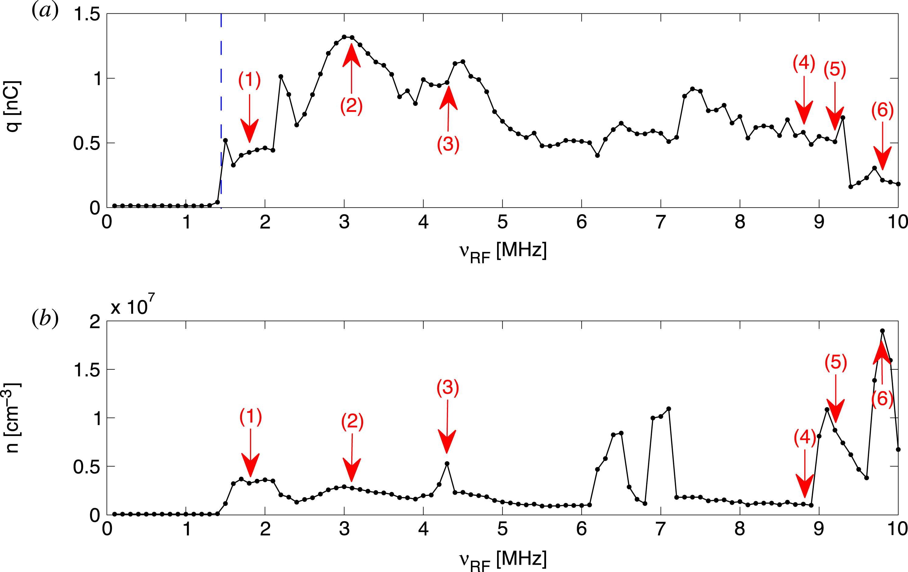
An example of the results obtained with the frequency-sweep looped measurement is summarized in figure 2. Figure 2(a) reports the total confined electron charge obtained as the sum of the pixel intensities of the CCD image after de-noising and intensity calibration. Figure 2(b) reports an approximate estimate of the corresponding mean electron density. This is calculated as the average density over the area of the image whose intensity is larger than half of the peak value. This may be a rather crude approximation for plasmas featuring low densities and irregular cross-sections, yet it allows us to recognize at a glance and unambiguously density peaks and to evaluate their core density. Some typical examples of plasmas that may be produced with the RF technique are indicated by red arrows and their corresponding CCD images are plotted in figure 3, where we can see: diffuse plasmas; narrow-radius columns, which are often surrounded by a lower-density background (case 3) or even halo rings (case 6) when they reach the highest attained densities (some $10^{7}~\text{cm}^{-3}$ ); quadrupole deformations (case 5).

Figure 2.

Example of frequency sweep measurement. Trap length $L_{trap}=570~\text{mm}$ , magnetic field $B=0.1~\text{T}$ , excitation amplitude $V_{RF}=1.5~\text{V}$ . (a) Total confined electron charge. The vertical dashed line indicates the threshold frequency ${\it\nu}_{thr}$ for plasma production and confinement. (b) Mean particle density. The transverse distributions of plasma corresponding to data points indicated by red arrows are plotted in figure 3.

Figure 3.

Examples of RF-generated electron plasmas. The axially-integrated transverse distributions of some of the plasmas from figure 2 are visualized as de-noised CCD images at plasma dump. Images numbered from 1 to 6 correspond to the frequencies 1.8, 3.1, 4.3, 8.8, 9.2 and 9.8 MHz, respectively (also indicated in figure 2).

Figure 4.

Repeatability test. The three frequency scan measurements were recorded during a single experiment/day with the same set of parameters, i.e. trapping length $L_{trap}=570~\text{mm}$ , magnetic field $B=0.1~\text{T}$ , excitation amplitude $V_{RF}=1.5~\text{V}$ . (a) Total confined charge. The vertical dashed line indicates the threshold frequency ${\it\nu}_{thr}$ for plasma production and confinement. (b) Mean particle density.

The diagrams in figure 2 also show another prominent feature of the RF plasma production, i.e. the existence of a distinct frequency threshold ${\it\nu}_{thr}$ beyond which the confined electron charge can be observed. This threshold is always present and we will investigate it further in the following, and we define ${\it\nu}_{thr}$ as the frequency corresponding to half of the charge level measured right after the first detectable rise in the charge versus frequency pattern.

2.2. Repeatability of RF-generated plasmas

Given the nature of the plasma generation process it is clear that the results will be extremely sensitive to the experimental conditions. Therefore the reproducibility of results must be assessed before any further data analysis and interpretation can be performed. We have partially addressed this issue in past experiments where repeated measurements had to be performed by means of a looped ‘create–hold and measure–dump’ procedure. This routine is typical of our experiments on low-order diocotron (Kelvin–Helmholtz) instabilities, for which we use a circular plasma column with a narrow radius and relatively high density ( $n\simeq 10^{7}~\text{cm}^{-3}$ ). In these cases we estimate that once the desired plasma is achieved and the set of parameters is fixed, the variations in the charge distribution at several successive plasma dumps are below few per cent if the experimental conditions are stable. Plasmas with different characteristics can still be randomly generated, but their occurrence is quite infrequent and they can easily be recognized by means of electrostatic or optical diagnostics and thus discarded (Maero et al. Reference Maero, Paroli, Pozzoli and Romé2011).

Figure 5.

Parametric measurement of plasma production against trapping length. (a) Total confined electron charge. The electron plasma produced by RF excitation is measured while slowly sweeping the RF frequency ${\it\nu}_{RF}$ at constant amplitude $V_{RF}=1.5~\text{V}$ and magnetic field $B=0.1~\text{T}$ . The measurement is repeated for different axial trap lengths. (b) The corresponding mean electron density is plotted.

Figure 6.

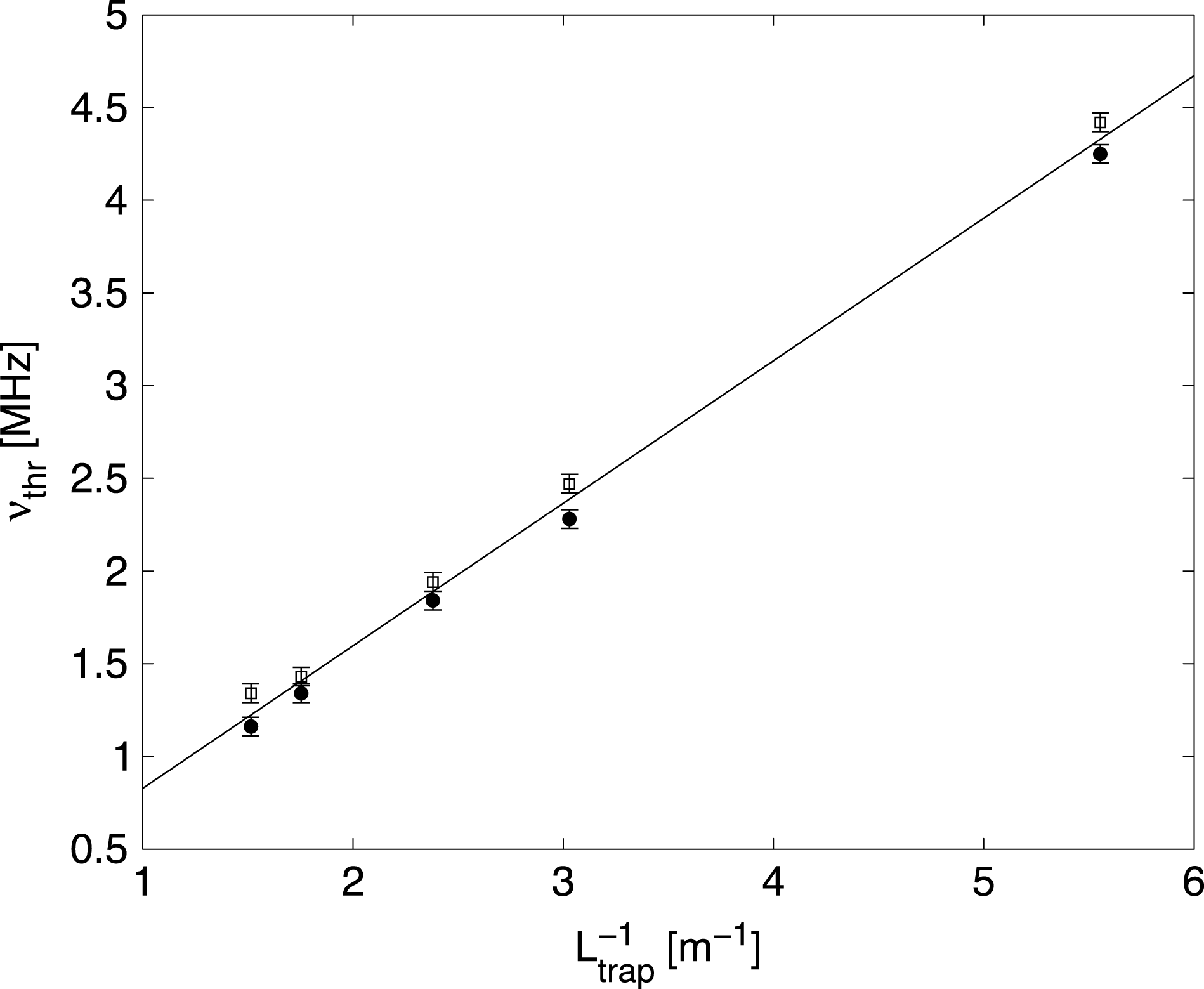
Threshold frequency versus the inverse of the trapping length. Two data sets (solid circles and hollow squares) from two distinct experiments are shown spanning trapping lengths $L_{trap}=180{-}660~\text{mm}$ . All experiments were performed at constant amplitude $V_{RF}=1.5~\text{V}$ and magnetic field $B=0.1~\text{T}$ . Error bars ( $\pm 50~\text{kHz}$ ) indicate the uncertainty of the threshold value in a single frequency sweep (as estimated in § 2.2). The solid line is a linear fit to all data.

Figure 7.

Parametric measurement of plasma production against the excitation amplitude. (a) Total confined electron charge. The electron plasma produced by RF excitation is measured while slowly sweeping the RF frequency ${\it\nu}_{RF}$ at constant trap length $L_{trap}=570~\text{mm}$ and magnetic field $B=0.1~\text{T}$ . The measurement is repeated for different excitation amplitudes $V_{RF}$ . (b) The corresponding mean electron density is plotted.

Figure 8.

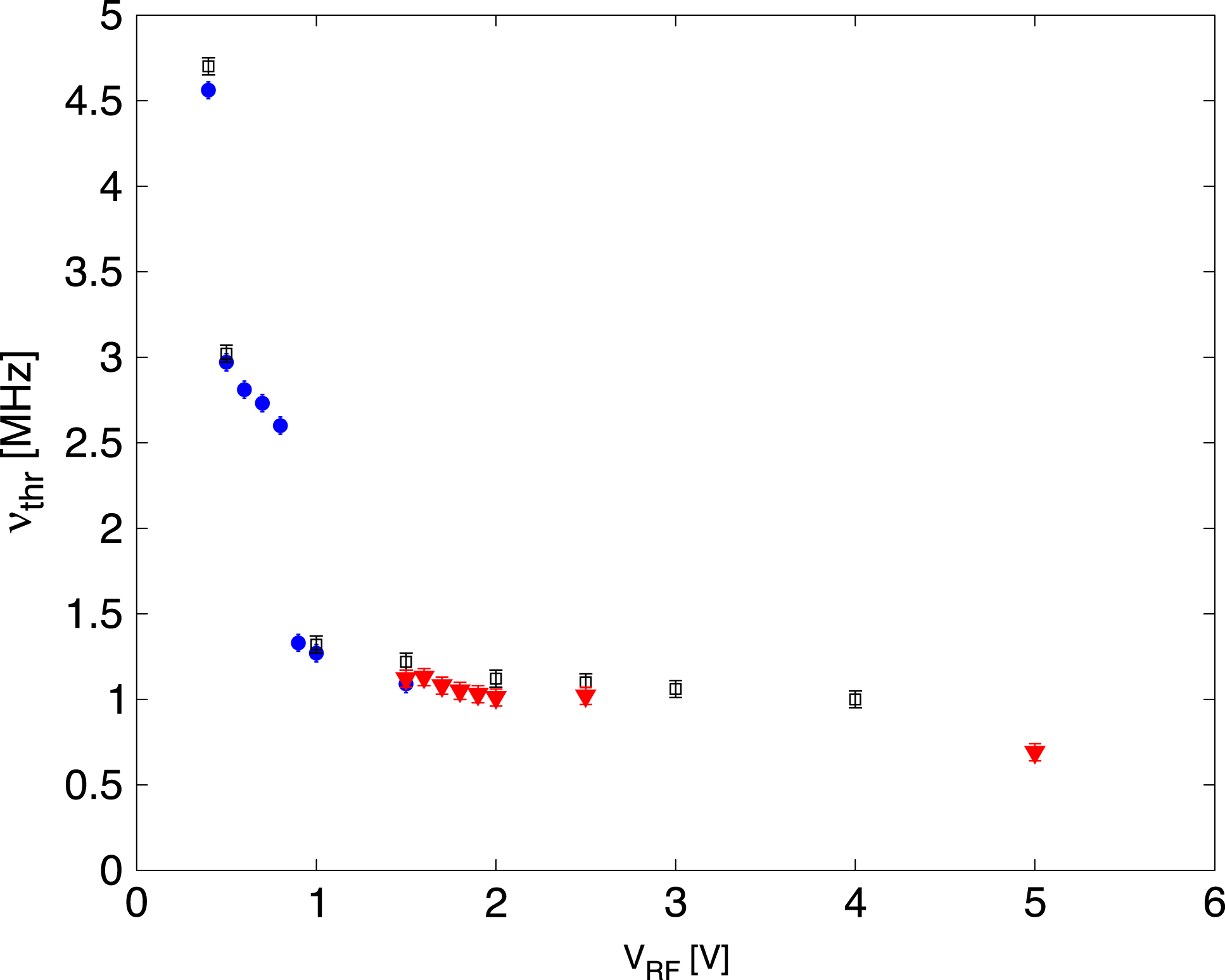
Threshold frequency versus the excitation amplitude. Data from three separate experiments (hollow black squares, solid blue circles, solid red triangles) are shown. All experiments were performed at constant trap length $L_{trap}=570~\text{mm}$ and magnetic field $B=0.1~\text{T}$ , changing the excitation amplitude $V_{RF}$ only. Error bars ( $\pm 50~\text{kHz}$ ) indicate the uncertainty of the threshold value in a single frequency sweep (as estimated in § 2.2).

Figure 9.

Parametric measurement of plasma production against the magnetic field intensity. (a) Total confined electron charge. The electron plasma produced by RF excitation is measured while slowly sweeping the RF frequency ${\it\nu}_{RF}$ at constant excitation amplitude $V_{RF}=1.5~\text{V}$ and trap length $L_{trap}=570~\text{mm}$ . The measurement is repeated for different magnetic fields. (b) The corresponding mean electron density is plotted.

Figure 10.

Threshold frequency dependence on the magnetic field intensity $B$ . All experiments were performed at constant excitation amplitude $V_{RF}=1.5~\text{V}$ and trap length $L_{trap}=570~\text{mm}$ and the magnetic field was varied in the range 0.06–0.16 T. The threshold frequency ${\it\nu}_{thr}$ is plotted against $B^{-2}$ together with a linear fit (solid line). Error bars ( $\pm 50~\text{kHz}$ ) indicate the uncertainty of the threshold value in a single frequency sweep (as estimated in § 2.2).

In the current experimental campaign, when repeating frequency scans at constant parameters the total charge trends are also fairly well reproduced over the course of a single experiment, typically spanning one day at most. As an example we may look at figure 4, showing three runs with excitation amplitude $V_{RF}=1.5~\text{V}$ in a 570 mm long trap and magnetic field $B=0.1~\text{T}$ . An estimate of the accuracy can be obtained by looking at the most prominent shapes in the curves, e.g. the first rise in total charge at the lower frequency threshold. This feature, as well as other recognizable patterns, may exhibit a horizontal (frequency) fluctuation of around $\pm 50~\text{kHz}$ , i.e. of about one data point. The vertical (total charge) fluctuation in these qualitatively repeatable patterns is of the order of 10 %.

More significantly, further deviations occur where single data points scatter widely from otherwise similar patterns. These events can be related to two different reasons: (a) the formation of a narrow, high-density plasma column; (b) the occasional presence of low-frequency (LF) modulation of the $m=1$ diocotron mode in a narrow column. The transition from a diffuse plasma to a narrow column is a complicated phenomenon whose discussion is left to a separate paper; for now, we simply remark that we have experimentally observed that this transition is not completely deterministic, i.e. it may require a varying amount of time to occur and also may not occur at all or shift to a slightly different frequency, probably depending on fluctuations of parameters beyond our control, namely the vacuum level or the ambient temperature. An example is the density peak at 7.8 MHz visible in figure 4, which is observed for one run only (red hollow squares). The LF modulation is a phenomenon observed in a previous paper (Paroli et al. Reference Paroli, Maero, Pozzoli and Romé2014) that is also accompanied by an oscillation of the electron column total charge and whose random initial phase results in a different charge detected over multiple measurements.

Measurements taken from different experiments/days may suffer from additional deviations (roughly of the same type and magnitude) due to the modification of experimental conditions, such as base pressure and temperature, which are subject to daily fluctuations depending on the environmental conditions and their feedback on the heat exchange in the magnet cooling system.

3.1. Trap length scan

We performed two separate experiments, each consisting of repeated RF frequency sweeps with different electrode pairs as trap endcaps, yielding trapping lengths equal to 180, 330, 420, 570 and 660 mm. All measurements were taken for a magnetic field of $0.1~\text{T}$ and an RF amplitude of 1.5 V, scanning the 0.1–10 MHz interval at a sweep rate of $20~\text{kHz}~\text{s}^{-1}$ (100 data points/sweep). Diagrams reporting the total charge and mean density for one of such sets are shown in figure 5 and indicate that the threshold frequency is progressively reduced as the trap length is increased. In particular, figure 6 shows that ${\it\nu}_{thr}$ scales with the inverse of the trapping length in the measurable range. This is reasonable as it is also the scaling of the axial bounce frequency in a flat-bottomed potential well. The energy of an electron oscillating with a bounce frequency equal to that of the threshold RF drive would be approximately 7 eV.

The total confined charge increases with the trapping length, which is reasonable as the capacity of the trap increases linearly. Indeed, the charge per unit length (linear charge density) yields similar values for all cases, with the exception of the shortest trap length, where the generation is less efficient and the frequency range where plasma is detected is strongly reduced (roughly 4–6.5 MHz). In this regard one should notice that for a very short length the approximation of a flat-bottomed longitudinal well and one-dimensional axial excitation becomes inappropriate. Increasing the trap length also increases the probability of observing high-density, narrow-radius plasmas.

3.2. RF amplitude scan

The excitation amplitude is an obvious parameter of choice, as it can be expected to have a strong qualitative and quantitative influence on the plasma generation. Figures 7 and 8 summarize the main results obtained from three different experiments covering the amplitude range 0–5 V. One of the experiments (solid red triangles in figure 8) was conducted at the usual resolution (sweep rate $20~\text{kHz}~\text{s}^{-1}$ , 100 data points) while the resolution was doubled (sweep rate $10~\text{kHz}~\text{s}^{-1}$ , 200 data points) in the other two (hollow black squares, solid blue circles in figure 8). All experiments covered the excitation frequency range ${\it\nu}_{RF}=0{-}10~\text{MHz}$ and were performed at constant trapping length $L_{trap}=570~\text{mm}$ and magnetic field $B=0.15~\text{T}$ .

Measurements show that electron plasmas can be detected using excitation amplitudes as low as 0.4 V and that the frequency threshold is reduced as $V_{RF}$ is increased. Looking at figure 8, where the dependence of the lower frequency threshold on $V_{RF}$ is plotted, one can notice that this trend is apparently not a continuous curve but rather a piecewise relation that tends to saturate at relatively large amplitudes.

In the same way, a larger $V_{RF}$ does not correspond to a systematic increase of the produced charge; on the contrary, with the saturation of ${\it\nu}_{thr}$ at large RF amplitudes the overall trend of the total confined charge shows comparable or even smaller values. A possible explanation may be related to the fact that higher amplitudes can lead to larger electron heating and in turn to increased axial losses.

3.3. Magnetic field strength scan

The dependence of the plasma generation on the strength of the axial magnetic field was also investigated. Figure 9 reports the confined electron charge and density measured in a 570 mm long trap and $1.5~\text{V}$ excitation for magnetic fields spanning the range 0.06–0.16 T. While the increase of $B$ has the effect of lowering the frequency threshold, it can be noticed that the overall charge versus frequency trend is largely unaffected in the ${\it\nu}_{RF}$ range above 3.5 MHz if we exclude the high-density peaks. On the contrary, the occurrence of such peaks is modified by the change of magnetic field intensity, although clear trends are not recognized.

Concerning the decrease of ${\it\nu}_{thr}$ for increasing magnetic field strength, one can observe that diffusion rates scaling with $B^{-2}$ can be expected in magnetized plasmas, and confinement times scaling with $B^{2}$ in trapped non-neutral plasmas were experimentally measured (Driscoll, Fine & Malmberg Reference Driscoll, Fine and Malmberg1986; Fajans Reference Fajans1999). The interpretation of ${\it\nu}_{thr}$ as an index of the balance between ionization and losses, leading in turn to a long-time effective confinement of the produced charge, supports the possibility of a similar scaling law. The measured threshold frequency is plotted in figure 10 against $B^{-2}$ along with a linear fit that shows that our data are consistent with the ${\it\nu}_{thr}\sim B^{-2}$ trend.