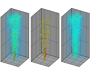

1. Introduction
Two-phase turbulent flows are widely used in engineering and environmental applications (Balachandar & Eaton Reference Balachandar and Eaton1993; Risso Reference Risso2018; Mathai, Lohse & Sun Reference Mathai, Lohse and Sun2020). Early studies of bubbly flow were conducted through current velocity measurements to investigate its ability as a breakwater (Evans Reference Evans1955; Taylor Reference Taylor1955). The applications of bubbly flow include aeration in reservoirs (McDougall Reference McDougall1978; Wüest, Brooks & Imboden Reference Wüest, Brooks and Imboden1992; Asaeda & Imberger Reference Asaeda and Imberger1993; Lemckert & Imberger Reference Lemckert and Imberger1993), oil and natural gas plumes to assess the fate of oil released from undersea oil explosions (Yapa, Zheng & Nakata Reference Yapa, Zheng and Nakata1999; Socolofsky & Adams Reference Socolofsky and Adams2002, Reference Socolofsky and Adams2003) and bubble plumes to inject liquid CO $_{2}$ directly into the deep sea as a means of mitigating the accumulation of greenhouse gases in the atmosphere (Caulfield et al. Reference Caulfield, Adams, Auerbach and Herzog1997; Socolofsky & Adams Reference Socolofsky and Adams2005). Two-phase bubbly flow studies have recently been inspired by the Deepwater Horizon oil spill, which was a disastrous accident (Yang et al. Reference Yang, Chen, Socolofsky, Chamecki and Meneveau2016).
In engineering applications, air injection is typically conducted through a sparger at the bottom of the system (Ziegenhein et al. Reference Ziegenhein, Zalucky, Rzehak and Lucas2016; Besagni & Inzoli Reference Besagni and Inzoli2017; Ansari & Nobes Reference Ansari and Nobes2020). Another way to create a two-phase mixed jet is by forming a gas–liquid mixture that has high momentum through an ejector that can produce small bubbles (Seo, Aliyu & Kim Reference Seo, Aliyu and Kim2018). Injection of gas–liquid mixtures has many advantages in terms of mixing enhancement. For example, even without porous materials, which have disadvantages when maintaining the system, small bubbles can be generated. Furthermore, the bubble size distribution associated with the mixing efficiency of the system is narrow and an air sparger is robust in generating small bubbles.
A gas–liquid ejector can generate a local low-pressure region where high-energy dissipation occurs, producing very fine bubbles (Cramers & Beenackers Reference Cramers and Beenackers2001; Zheng et al. Reference Zheng, Yao, Guo, Bi and Li2010; Terasaka et al. Reference Terasaka, Hirabayashi, Nishino, Fujioka and Kobayashi2011; Aliyu et al. Reference Aliyu, Seo, Kim and Kim2018; Seo et al. Reference Seo, Aliyu and Kim2018). For bubbly jets with bubble generators, the co-flow suppresses the coalescence of bubbles near nozzles and accelerates bubble separation (Muilwijk & Van den Akker Reference Muilwijk and Van den Akker2019). In this case, the plume spreading of the turbulent bubbly mixed jet can be governed by different physical processes from a classical bubble plume. However, detailed physical mechanisms in a turbulent dilute bubbly mixed jet have not been investigated so far. The classic single-phase plume is self-similar and spreads linearly with height. The turbulent entrainment determines the increase in liquid volume flux within the plume and scales according to the centreline velocity of the plume. However, a two-phase bubbly plume has a variable entrainment coefficient (Milgram Reference Milgram1983; Seol et al. Reference Seol, Bhaumik, Bergmann and Socolofsky2007), and it may not be strictly self-similar but retains many characteristics of integral properties of plumes.
Slip velocity induces two-phase plumes that deviate from self-similarity in the integral framework. In a single-phase plume, the plume characteristics depend on the length scale  $z$ (which is the distance from the plume source) and the initial kinematic buoyancy flux
 $B_0$. In a two-phase plume,
 $B_0$ and the slip velocity
 $U_{slip}$ can be combined to generate a secondary length scale (e.g.
 $B_0$/
 $U_{slip}^3$), which breaks the self-similarity requirement (Bombardelli et al. Reference Bombardelli, Buscaglia, Rehmann, Rincón and García2007). Typically, the slip velocity in a gas phase is a function of several parameters, such as the density difference between liquid and gas phases, viscosity, interfacial tension of the bubble and the size of the bubble. Although the slip velocity is the main cause of breaking the self-similarity of bubbly flow, previous studies have simply estimated the bubble slip velocity based on the average equivalent bubble diameter (Motarjemi & Jameson Reference Motarjemi and Jameson1978; Seol et al. Reference Seol, Bhaumik, Bergmann and Socolofsky2007).
Many experimental studies measured the exact bubble slip velocity. Experimental studies to investigate the dynamic behaviour of bubbles in bubbly flows have been conducted in invasive and non-invasive manners. Fibre optic probes are typically used for invasive measurement to obtain local phase properties in bubble plumes at high bubble fractions (Lima Neto, Zhu & Rajaratnam Reference Lima Neto, Zhu and Rajaratnam2008; Besagni, Guédon & Inzoli Reference Besagni, Guédon and Inzoli2015). However, the flow structure can be changed by the inserted sensors, so invasive methods should be used carefully.
Acoustic Doppler velocimetry (ADV) is a measurement method involving partial invasiveness and requires sufficient distance between the probe and the sample volume. The ADV method can provide turbulent statistics at relatively large measurement volumes (Lai & Socolofsky Reference Lai and Socolofsky2019). Laser Doppler velocimetry (LDV) has a basic principle similar to that of ADV but provides a non-invasive method for measuring flow velocity while having a small volume of measurement (Sun & Faeth Reference Sun and Faeth1986). Although LDV is non-invasive, it requires a clear line of sight, so the sample volume usually cannot be far from the edge of the bubbly region. The ADV and LDV techniques require multiple verifications and optimization for bubble measurement due to the scattering and morphological considerations of bubbles (Groen, Mudde & Van Den Akker Reference Groen, Mudde and Van Den Akker1999; Lai & Socolofsky Reference Lai and Socolofsky2019).
The most common optical method for measuring bubbly flows is bubble shadowgraphy, which records two-dimensional (2-D) bubble images (Xu et al. Reference Xu, Aliyu, Seo, Wang and Kim2018; Echeverría et al. Reference Echeverría, Porta, Stern and Guzmán2020; Saini & Banerjee Reference Saini and Banerjee2021). The positions and equivalent diameters of bubbles can be obtained in laser sheets to calculate the bubbles’ rising velocity and equivalent size. This means that it is difficult to obtain the exact distribution of bubbles that exhibit three-dimensional (3-D) characteristics.
Wang, Lai & Socolofsky (Reference Wang, Lai and Socolofsky2019) used a stereo imaging system to quantify the bubble size, void fraction and rise velocity of bubbles using two cameras. Another optical method is the planar laser-induced fluorescence method, which uses fluorescence around bubbles and a laser to obtain bubble images in a target plane (Siddiqui et al. Reference Siddiqui, Munir, Heikal, de Sercey, Aziz and Dass2016; Seo & Kim Reference Seo and Kim2021). Two-dimensional particle image velocimetry and particle tracking velocimetry are also applied to understand the flow characteristics and mixing characteristics of various two-phase flows in measured planes (Gui & Merzkirch Reference Gui and Merzkirch1996; Delnoij et al. Reference Delnoij, Westerweel, Deen, Kuipers and van Swaaij1999; Deen Reference Deen2001; Lindken & Merzkirch Reference Lindken and Merzkirch2002).
The difficulty of measurement in two-phase flows is that a dispersed phase with 3-D behaviour and a continuous phase with turbulent characteristics exist together (Balachandar & Eaton Reference Balachandar and Eaton1993; Risso Reference Risso2018; Mathai et al. Reference Mathai, Lohse and Sun2020). Due to this limitation, turbulent bubbly flow studies continue using 2-D measurements or even separately measure each phase because the identification of gas and liquid phases is very difficult in the same image (Seo & Kim Reference Seo and Kim2021). Masuk, Salibindla & Ni (Reference Masuk, Salibindla and Ni2021) presented simultaneous 3-D measurements of deformable finite-sized bubbles and surrounding turbulent flows based on shadow images of bubbles and particle tracking velocimetry. They found that orientations of bubbles are linked to two key mechanisms that drive bubble deformation: the turbulent strain rate and slip velocity between the two phases. However, their measurements are limited to a small volume which contains few bubbles and hundreds of velocity vectors. When measuring each phase separately, it is difficult to determine the interaction between the liquid flow and the bubble behaviour. Thus, a challenge in measurement of two-phase flow is determining the interaction between each phase by simultaneously measuring gas and liquid phases.
Thus, an accurate phase-separation method should be developed to measure the turbulent characteristics of the liquid phase and the 3-D behaviour of the bubbles. To the best of our knowledge, there is no report on particle-based 3-D velocity measurements of turbulent bubbly jets. Therefore, the first objective of this study is to propose a novel time-resolved 3-D simultaneous measurement method to obtain instantaneous and time-averaged 3-D velocity information about the continuous phase and dispersed phase of a turbulent bubbly jet. This simultaneous measurement technique for gas and liquid phases is important for clearly evaluating the interaction between dispersed phase and continuous phase required for the integral frameworks, the mean flow characteristics of the plume and the entrainment coefficients. Lagrangian particle tracking (LPT) using the Shake-The-Box (STB) method (Schanz, Gesemann & Schröder Reference Schanz, Gesemann and Schröder2016) is used to measure 3-D flow characteristics. The STB method allows the extraction of time-resolved 3-D trajectories of tracer particles and bubbles. Basically, there are small local scales and larger scales in chemical reactors. The former influences the latter not only in terms of mass transfer, but also in terms of the fluid dynamics. In this study, we mainly focus on the fluid dynamics with relatively larger-scale phenomena.
The second objective is to verify theories based on integral frameworks for bubbly jets and plumes with 2-D measurements. The obtained 3-D flow-field data were analysed to determine the time-averaged flow characteristics of a dilute bubbly mixed jet. Important parameters were compared with those of previous works, including the velocity profiles, slip velocities, volume fractions, entrainment coefficients and scaling.
2. Methods
2.1. Experimental set-up
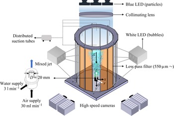
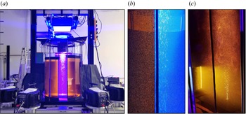
Figure 1 shows a schematic of the LPT experiment for simultaneous 3-D measurement of liquid and gas phases. Figure 2(a) shows a photograph of the main experimental set-up. The experiment was conducted in a water tank with a height of 1 m, which was constructed of 16 glass plates to ensure orthogonal viewing conditions for each camera to avoid optical distortions. The system diameter was 0.1 m. So, the aspect ratio of the experimental system, which means the ratio of initial liquid level to system diameter, was 10.0. Fluorescent orange polyethylene microspheres (Cospheric, 1.00 g cm $^{-3}$, 53–63
 $\mathrm {\mu }$m) were used as tracer particles for the liquid phase. They were illuminated from above, using a volumetric illumination by three arrays of blue light-emitting diodes (LEDs; Lavision LED-Flashlight 300) and a 1000 mm collimating lens. A circular passe-partout was applied to achieve a cylindrical illumination. Low-pass plate optical filters (550
 $\mathrm {\mu }$m) were attached to each glass measurement plane to suppress the reflection and refraction signals of bubbles by the blue light source and to suppress any reflections. Figure 2(b) shows a photograph of two glass plates of the water tank, one of which is equipped with an optical filter. It is evident how the blue light is filtered out, eliminating any background light and suppressing the strong reflections on the bubble surfaces. Two white LED arrays were installed at two opposite sides of the tank. As seen in figure 2(c), these arrays have a streamwise extent of approximately 250 mm and were positioned at the bottom part of the tank. In the illuminated region, the bubbles become visible even through the filters. As argued above, this set-up allowed fine tuning of the ratio of light reflected by the bubbles and scattered by the particles, being recorded by the cameras.
Experimental set-up for simultaneous measurement of liquid- and gas-phase flows.

Photographs of the set-up. (a) Overview showing the tank, the blue illumination for the fluid phase, the orange filters applied to four of the glass windows and the camera set-up. (b) Simultaneous view through two glass plates with and without filter, illustrating the filtering effect on the bubbles (only blue LEDs on). (c) View through two of the orange Plexiglas filters, illustrating the effect of bubble visibility by the white illumination, coming from the side at the bottom part of the tank (blue and white LEDs on).

The 3-D motion of particles and bubbles was recorded at a sampling frequency of 350 Hz using four cameras (Phantom v2640). The cameras were equipped with 60 mm Zeiss Makro-Planar lenses, set to  $F_\# = 16$. Because of the cylindrical illumination, no Scheimpflug adapter was needed. To obtain statistics, 36 300 images were acquired in 363 chunks of 100 images each, with a chunk period of 0.286 s. To obtain clear images without blur, the blue and white LEDs were operated at a duty cycle of 1:10 (being active for 280
 $\mathrm {\mu }$s at a repetition rate of 350 Hz).
The bubble generator was built into the bottom wall of the water tank. To generate small monodispersed bubbles, the bubble generator has six 32-gauge needles in the nozzle tube. The needles have an inner diameter of 0.089 mm, and their tips were ground to flatten them. The needles were assembled with  $1/8''$ stainless tubes to connect them with an air pocket in the bubble generator. The small monodispersed bubbles are generated by shear cutting between the liquid and bubbles that form at the very small orifices of the needles (Seo & Kim Reference Seo and Kim2021).
Knowledge of bubble size distributions is of great importance for the design of corresponding facilities, for the optimization of processes and for a safe operation. The spatial distribution of bubbles is influenced by the momentum exchange between the continuous liquid phase and the dispersed bubbles. For example, in bubble columns, the hole diameters impose the initial bubble size distribution and, thus, the prevailing bubble size distributions across the bubble column, thus determining the prevailing flow regimes such as homogeneous monodispersed and homogeneous polydispersed (Hessenkemper et al. Reference Hessenkemper, Ziegenhein, Rzehak, Lucas and Tomiyama2021).
The bubble size distribution from the bubble generator was analysed in our previous study (Seo & Kim Reference Seo and Kim2021). The bubble size has a Gaussian distribution with standard deviation of  $10\,\%$. The bubble drag is often stated as the most important interaction force since it determines the momentum exchange due to the slip velocity between both phases. However, also the lift force has a major influence on the lateral void distribution in bubbly flows and is supposed to stabilize or destabilize a flow regime depending on its sign (Hessenkemper et al. Reference Hessenkemper, Ziegenhein, Rzehak, Lucas and Tomiyama2021). In general, the lift force acting on small, spherical bubbles that pass a shear field is different from that acting on larger, ellipsoidal bubbles. Spherical bubbles are pushed into the direction of decreasing liquid velocity and form a wall-peak void distribution in a co-current upward flow.
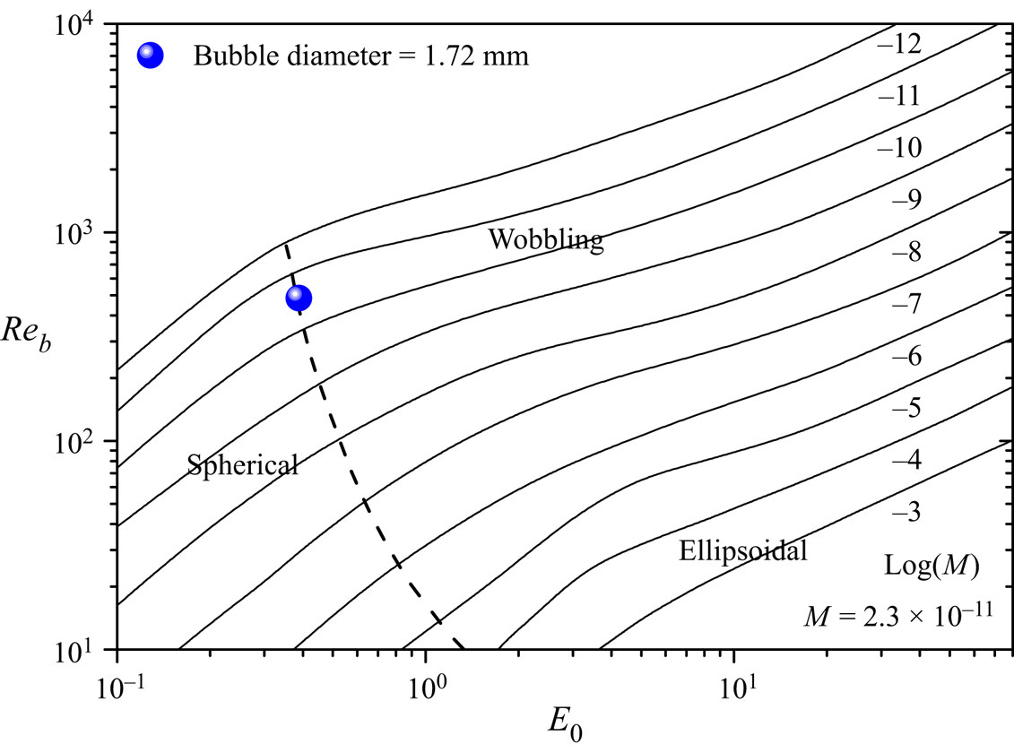
Monodispersed bubbles of  $1.72\pm 0.17$ mm in diameter were formed by the bubble generator (Seo & Kim Reference Seo and Kim2021) to suppress the flow characteristics that can be attributed to the various sizes of bubbles (Fujiwara, Minato & Hishida Reference Fujiwara, Minato and Hishida2004). In this study, the size of the bubbles was small enough to avoid wobbling regime of bubble shape and we measured accurate 3-D bubble velocity fields. Similar to the experimental work performed by Muilwijk & Van den Akker (Reference Muilwijk and Van den Akker2019), co-flow due to water supply has the effect of separating bubbles from needles. An air compressor was used to supply air to the bubble generator, and the air flow rate was manipulated using a pressure regulator and a tachometer (Dwyer RMA-151). The air void fraction (
 $Q_g/Q_l$) at the inlet nozzle was limited to less than
 $1\,\%$. To prevent inclination of the bubble plume, four distributed suction tubes were installed near the free surface, and ground plates were installed on the bottom surface of the water tank to prevent unintended boundary effects.
The quantitative presentation of bubble shape regime can be illustrated by three non-dimensional parameters: Reynolds number,  $Re_b = \rho d_b U_s /\mu$, where
 $d_b$ is the diameter of a bubble,
 $U_s$ is the slip velocity and
 $\mu$ is the dynamic viscosity of surrounding fluid; Morton number,
 $M = g \mu ^4 \Delta \rho / \rho ^2 \sigma ^3$, where
 $\Delta \rho = \rho - \rho _b$ and
 $\sigma$ is the interfacial tension; and Eötvös number,
 $E_o = g \Delta \rho d_b^2 / \sigma$. The slip velocity used to calculate the Reynolds number is obtained from figure 13(b). Values for our experiments are shown in figure 3 along with the shape regime classification in Clift, Grace & Weber (Reference Clift, Grace and Weber1978). Figure 3 demonstrates that the observed bubbles are near the spherical regime of the bubble theory.
Experimental set-up for simultaneous measurement of liquid- and gas-phase flows.

Both Cartesian and cylindrical coordinates were used in the evaluation. In the Cartesian coordinate system,  $x, y$ and
 $z$ represent the spanwise direction, image-depth direction and streamwise direction, respectively (see figure 1). In the cylindrical coordinate system,
 $r$ is the radial coordinate and
 $\theta$ is the horizontal angle measured from the
 $y$ axis. The origin of both coordinate systems is the centre of the nozzle exit. The measured volume is approximately 280 mm (width)
 $\times$ 260 mm (depth)
 $\times$ 300 mm (height). The spatial resolution of each camera is 73
 $\mathrm {\mu }$m pixel
 $^{-1}$. The measurement area along the
 $z$ direction (height) covers approximately 15 times the outlet diameter of the bubble generator (
 $z = 15D,\ D = 20$ mm). Gravity acts in the negative
 $z$ direction.
The vertical length scale above a plume source was selected in various ways in the plume analysis. One of the most common and simplest ways of selecting the height of the evolution is based on the outlet diameter of the jets or various length scales in a single-phase plume (Milgram Reference Milgram1983). Another length scale is the Morton length scale from the ratio of the momentum and buoyancy flux. According to the description of Morton (Reference Morton1959), the balance of the source flux is expressed using the following jet momentum length scale:
 \begin{equation} L_{m} = {M_{0}^{3/4}}/{B_{0}^{1/2}}, \end{equation}
where  $M_0$ is the momentum flux and
 $B_0$ is the buoyancy flux from the source.
In this study, the jet momentum length scale was calculated as  $L_{m} = 68$ mm. With respect to the jet momentum length scale, the measurement area transitioned from where the initial momentum was dominant (
 $z < L_m$) to the jet plume (
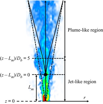
 $L_m < z < 5 L_m$) (Fisher et al. Reference Fisher, List, Koh, Imberger and Brooks1979; Hunt & Kaye Reference Hunt and Kaye2001). Delineation of the momentum-dominated (jet-like) region from the buoyancy-dominated (plume-like) region is important because dominant length scales are different. In this paper, the jet-to-plume transition length scale
 $L_m$ from the single-phase jet flow in the literature was used for delineation.
Table 1 shows the experimental conditions used in this study, where  $Q_l$ is the volumetric flow rate of liquid,
 $Q_g$ is the volumetric flow rate of gas,
 $D$ is the diameter of bubble generator outlet and
 $\gamma$ is initial air void fraction of bubbly jet. Reynolds number (
 $Re$) is defined as
 \begin{equation} Re = {\rho UD}/{\mu}, \end{equation}
where  $\rho$ is the density of water,
 $U$ is the outlet velocity of bubbly jet from bubble generator and
 $\mu$ is the dynamic viscosity of water. When calculating the Reynolds number, the contribution of the air is ignored due to the low void fraction.
Experimental conditions used in this study.

2.2. Phase separation and data processing
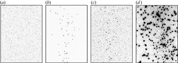
The objective of this section is to develop a phase-separation method. To this end, a combination of fluorescent tracer particles, spectral filters and two different light sources is applied. A major problem when trying to simultaneously capture the images of millimetre-sized bubbles and of small seeding particles (around  $50\,\mathrm {\mu }$m) is the high dynamic range of the scattered and reflected light. While the bubbles reflect light in high intensities, both on the outer and the inner interface (thus they are imaged as two bright peaks in close proximity), the particles scatter light at much lower intensity. In a previous attempt, only a single illumination device was applied (a green LED array). Once the LEDs were operated such that the particles were visible to the cameras, the bubbles were significantly overexposed, preventing any reliable detection (see figure 4d). Based on this experience, we extended the set-up: the particles were exchanged for fluorescent ones, being excited by a blue LED. Filters were installed on the glass walls of the tank, allowing the emitted orange light to pass. This way, the blue light, reflected by the bubbles, could be completely blocked. In order to get a signal from the bubbles, an additional array of white LEDs was installed. The orange part of the spectrum emitted from these LEDs was able to pass the filters and by varying the brightness of the white LED, the intensity of the bubble images could be tuned. In order to achieve a good separation from the particles, a recorded intensity of around three times the intensity of the particle images was chosen.
Excerpts of camera images for different illumination configurations. (a) Only blue LEDs on: only fluorescence light of the particles is visible. (b) Only white LEDS on: only bubbles are visible due to light scattering and partly passing through the orange filters; particles are invisible due to small size and low light intensity. (c) Blue and white LEDs on: particles and bubbles visible. (d) Camera image without filters, demonstrating the bubble overexposure at light levels needed to resolve the particles.

In order to separate the bubbles from the particles in the tracking process, the images were first treated by correlating a calibrated two-peak kernel, followed by Gaussian blurring, allowing the two glare points of the bubbles to merge to a single peak and simultaneously decreasing the intensity of the particle images. In the resulting images, the bubble peaks could be easily identified, triangulated and tracked. In a second step, the bubble images were eliminated from the original camera images by back-projecting the known bubble positions onto the cameras and subtracting a Gaussian peak. Gaussian peak diameter is close to the bubble diameter, which is 1.7 mm. The monodispersed and almost non-deformable bubbles have a size distribution of  $1.7\pm 0.17$ mm. The size of a tracer particle is 0.05 mm, so that the particles located very close to the bubbles at less than three particle diameters can be eliminated. In this experiment, we could not find particle erase because the particle loading rate and void fraction are very low. The result is a camera image with undisturbed particle peaks and removed bubble images, on which the tracking of the tracer particles could be conducted.
The phase separation and data processing procedure to obtain the 3-D velocity field using LPT with STB are described in the following steps. The STB method relies on predicting the position of already tracked particles and refining the found position by an image-matching scheme involving shaking all particles within the measurement box until they fit the images. New particles entering the measurement domain are identified using triangulation on the residual images.
Before recording images to obtain particle and bubble positions, optical calibration was performed to accurately triangulate the position of a particle from all 2-D images obtained from four cameras in 3-D space. To this end, a two-plane calibration plate was placed above the nozzle outlet. The geometric calibration accuracy was improved by applying volume self-calibration (Wieneke Reference Wieneke2008) and calibration of the optical transfer function (Schanz et al. Reference Schanz, Gesemann, Schröder, Wieneke and Novara2012). The calibration error was reduced from 1 pixel to about 0.1 pixel.
As introduced in § 2.1, a combination of fluorescent particles, optical filters and illumination with two different light sources was used to adjust the dynamic range between bubbles and tracer particles. Fluorescent particles were used as tracers of the fluid phase, which have a maximum excitation peak at 577 nm and an emission peak at 606 nm in the orange range. A blue LED with a wavelength of 450 nm was used as the light source for the fluorescent particles. The flow is viewed by four cameras through orange colour filters on the glass plates of the water tank (see figure 2a,b). Figure 4(a) shows a camera image in a situation where only the blue LEDs are active. Only the fluorescent particles are imaged. In order to simultaneously image the bubbles in an intensity-controlled fashion, two white LED arrays are used, illuminating the volume from the side (see figure 2c). After tuning the intensity of the white LEDs, such that the bubbles are optimally imaged, the tracer particles become invisible due to their small size (figure 4b). Operating both kinds of LEDs finally allows a balanced imaging of both particles and bubbles (figure 4c). Compared with the images captured in a previous experiment, which relied on only a single illumination for both phases (figure 4d), the improved imaging of the bubbles is evident. The described careful image acquisition procedure lays the foundation for the separate determination of the two phases. However, due to specific imaging of the bubbles (two glare points per bubble), a multi-step approach with specialized image preprocessing had to be carried out.
Various image-processing methods have been used in the past to identify bubble signals and separate the phases. Gui & Merzkirch (Reference Gui and Merzkirch1996) and Gui, Lindken & Merzkirch (Reference Gui, Lindken and Merzkirch1997) used size differences between a bubble and a tracer particle, while Sakakibara, Wicker & Eaton (Reference Sakakibara, Wicker and Eaton1996) used grey-scale intensity differences to distinguish the two phases. Other possible methods include applying a median filter (Kiger & Pan Reference Kiger and Pan2000), an edge detection algorithm (Brücker Reference Brücker2000) or digital masking (Gui & Merzkirch Reference Gui and Merzkirch1996; Lindken, Gui & Merzkirch Reference Lindken, Gui and Merzkirch1999; Grota & Strauß Reference Grota and Strauß2000). Bubble signals can be removed during data processing using ensemble correlation according to the slip velocity (Deen, Westerweel & Delnoij Reference Deen, Westerweel and Delnoij2002). The bubble phase and liquid phase have different correlation peaks in the correlation field, so the higher the velocity caused by a bubble, the more separable it can be.
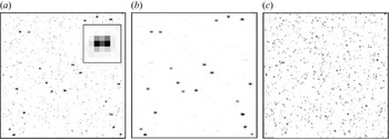
In this study, the bubble field is tracked using STB on preprocessed images in the first step, followed by STB tracking of the particles on the original camera images with removed bubble reflections. In order to successfully triangulate (and then track) a bubble from the recorded images, the following image preprocessing was applied. The image of a single bubble consists of two glare points, which are the reflections on the inner and the outer interface of the bubble. The original camera view in figure 5(a) shows such bubble images, as well as the lower-intensity particle field. Figure 5 is a zoomed image ( $50 \times 50$ pixels) of a specific area from the original image (
 $3820 \times 4096$ pixels). The distance of the two glare points is determined by the bubble size, given a fixed magnification, and the angle of the camera relative to the white LED illumination. The different cameras see the glare points of a single bubble originating from different 3-D positions, due to the geometric properties of the reflections in relation to the space angle in which the cameras are positioned. Therefore, direct triangulation and tracking of the two glare points are not possible. In order to merge the two glare points into a single peak, a 2-D kernel was calibrated for each camera, which constitutes the average image of a bubble within each camera (see inset in figure 5a). The camera images were correlated with this kernel, yielding a central peak with weaker side peaks. In order to enhance the central peak, the image was squared (enhancing contrast) and finally a Gaussian smoothing was applied. An example of the resulting image is given in figure 5(b), showing an easily identifiable peak in the central position between the former glare points. From these images, the bubble positions could be triangulated and STB was able to track most bubbles for their entire trajectory through the measurement volume. Typically, between 200 and 300 bubbles were instantaneously tracked.
Image processing for bubble and particle tracking. (a) Original camera image (only minimum subtracted); the inset shows the double-peak kernel used for image processing. (b) Preprocessed image by convolution with double-peak kernel, squaring and Gaussian smoothing – used for bubble tracking. (c) Original camera image with bubble images removed by reprojection and subtraction of tracked bubbles – used for particle tracking. Different intensity scales are used between the three images for the sake of clarity.

Once the bubble field was tracked, the images of the bubbles were eradicated from the camera images by back-projecting the found 3-D positions onto the different cameras using the 3-D calibration and subtracting an extended Gaussian peak around the projection point. As a result, the image of the bubbles is completely removed and STB tracking can be performed on pure particle images (see figure 5c). The particle position reconstruction with STB was performed using advance iterative particle reconstruction (Wieneke Reference Wieneke2012; Jahn, Schanz & Schröder Reference Jahn, Schanz and Schröder2021). The measurement area exhibits a high dynamic velocity range: regions with low velocities (large quiescent parts surrounding the plume) are in proximity to regions with at least an order of magnitude higher velocity in the centre of the plume. In order to best capture the particle trajectories in all regions, STB tracking was performed using the recently introduced ‘variable-timestep’ mode (Schanz, Novara & Schröder Reference Schanz, Novara and Schröder2021), which employs an iterative tracking process with decreasing time separations. In this way, the slowest particles are tracked in a first step, with faster and faster particles being added in subsequent iterations. Three iterations with time separations of  $\Delta _s = 11$ time steps,
 $\Delta _s = 6$ time steps and
 $\Delta _s = 1$ time step are performed. Typically, around 90 000 particles could be tracked instantaneously. For further separation of the particle and bubble tracking, a maximum particle velocity of 0.25 m s
 $^{-1}$ was enforced.
After the tracking process of bubbles and particles, a temporal filter using third-order B-splines with optimal weighting coefficients was applied to determine velocity and acceleration of the tracked particles. The results were used within the averaging procedure and as input for the FlowFit interpolation method (Gesemann et al. Reference Gesemann, Huhn, Schanz and Schröder2016). To reconstruct the velocity field as a continuous function based on scattered particle data, we model this function as a uniform cubic B-spline and compute the weighting coefficients of the B-spline's compact base functions by minimizing a cost function (Gesemann et al. Reference Gesemann, Huhn, Schanz and Schröder2016). This cost function is the sum of different kinds of squared and weighted errors including the errors between reconstructed velocity and measured velocity at the particle locations. As regularization, the curvature at each grid point is part of the cost function with a selectable but typically low weight. This results in an optimization problem with a unique solution. The estimated errors in velocity quantification are less than  $0.5\,\%$ (Gesemann Reference Gesemann2021). The optimal weighting coefficients were determined using the position amplitude spectrum of the raw tracks, as given in Gesemann et al. (Reference Gesemann, Huhn, Schanz and Schröder2016) and Gesemann (Reference Gesemann2021). The same analysis allows the determination of the average position error of the particles before and after fitting for each coordinate individually. The raw positions showed an average reconstructed error of approximately (13, 18, 11)
 $\mathrm {\mu }$m for the (
 $x, y, z$) coordinates. The differences between the coordinates can be attributed to the in-line camera set-up, which allows an optimal viewing of the streamwise
 $z$ coordinate by all cameras, while the depth coordinate (
 $y$) is reconstructed with the highest inaccuracy due to the relative angle of the cameras. After fitting, the error is lowered to approximately (6, 8, 5)
 $\mathrm {\mu }$m for (
 $x, y, z$). The same treatment for the bubble trajectories yields average accuracies of (25, 25, 15)
 $\mathrm {\mu }$m. The reduced relative accuracy of the
 $x$ coordinate is attributed to the double glare points, which are oriented in this direction. After fitting, the bubble position uncertainty is reduced to (12, 12, 7)
 $\mathrm {\mu }$m.
For the determination of flow structures, the discrete particle field was interpolated on an Eulerian grid using the FlowFit data assimilation method (Gesemann et al. Reference Gesemann, Huhn, Schanz and Schröder2016). To this end, a grid of third-order B-splines with a spacing of 2 mm is created and the B-spline coefficients are iteratively fitted to the discrete values of velocity and acceleration provided at the particle locations. A further increase in spatial resolution is achieved by including incompressible Navier–Stokes constraints within the cost function of the nonlinear data assimilation process. For FlowFit, the velocity and acceleration vectors of both phases have been used as input with the argument that the liquid phase at the two stagnation points at the upper and lower end of each bubble behaves identical to the bubble dynamics, although slip velocities are present at the bubble sides. However, the unwanted bubble footprints were removed to obtain a more clear instantaneous velocity vector of the continuous phase. A rough criterion is specifying an allowable velocity range for the fluid. In this study, the maximum allowable vertical velocity of the liquid was set to 0.25 m s $^{-1}$ and we ignored the liquid velocity at the stagnation points.
The post-processing is key to the quality of space-filling velocity and acceleration field reconstruction from the scattered particle data. Ehlers, Schröder & Gesemann (Reference Ehlers, Schröder and Gesemann2020) described a straightforward extension of the recently developed data assimilation scheme FlowFit, which applies physical constraints from the Navier–Stokes equations in order to simultaneously determine velocity and acceleration fields as solutions to an inverse problem. The velocity bias error typically attains values within  $0.5\,\%$ of the fluid velocity. Bin-averaging of the Lagrangian particle and bubble track velocity vectors was performed separately over all 36 300 time steps to obtain the ensemble-averaged velocity field. As a result, the averaged velocity fields for the liquid phase and the bubbles’ rising velocity field can be obtained. The resolution of the Cartesian grid used for FlowFit and bin-averaging was 2 mm.
3. Results and discussion
3.1. Lagrangian particle tracking results
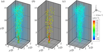
Figure 6 shows the simultaneous measurement and phase-separation results of the 3-D LPT with STB of the bubbles and water (see supplementary movie 1 available at https://doi.org/10.1017/jfm.2022.301). As shown in figure 6(a), the 3-D flow fields of the dispersed phase and the continuous phase were successfully measured simultaneously. Figures 6(b) and 6(c) present the scatter of the bubbles and the velocity vectors of the continuous phase, respectively. Velocity magnitudes of the bubbles and liquid phase are colour-coded. Continuous and dispersed phases are separated clearly. The flow of the bubbles is faster than the water flow. The bubbles are shown 2.5 times larger than their actual size for easier identification.
Lagrangian bubble–particle tracking and phase separation results for (a) simultaneous measurement, (b) bubbles and (c) particles.

At the outlet of the jet nozzle, water and bubbles are ejected together, but as they go downstream, the initial momentum is dissipated, and the jet becomes a bubble plume where water is entrained by rising bubbles. As a bubble rises, it spreads to the radial direction, and the volume of the two-phase bubbly jet also increases. The flow of the liquid phase has a higher velocity magnitude closer to the centre, which resembles a single-phase turbulent jet. Turbulent fluctuations are generated by shear layers of water jet and irregular bubble motions. When the air bubbles reach the terminal velocity downstream, the bubble velocity stays constant, which means that the surrounding fluid is continuously entrained by the bubble plume.
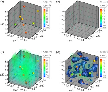
Recently, Masuk et al. (Reference Masuk, Salibindla and Ni2021) presented simultaneous 3-D measurements of deformable finite-sized bubbles and surrounding turbulent flows based on shadow images of bubbles and particle tracking velocimetry. However, their measurements are limited to a small volume which contains few bubbles and hundreds of velocity vectors. The research is meaningful for understanding local flow physics regarding deformation of bubbles associated with 3-D flow fields. Our research aims to measure the whole field of the turbulent bubbly jet by measuring instantaneous 3-D velocity fields of bubbles and continuous-phase simultaneous. It is needed to verify that the current measurement can resolve turbulence structures in the bubbly jet and plume. We magnify a small volume in figure 6 to show detailed scales of velocity vectors. Figure 7 shows instantaneous velocity field in a volume of  $20\,{\rm mm}\times 20\,{\rm mm}\times 20\,{\rm mm}$ which corresponds to a volume of
 $6 < z/D < 7,\ -0.5 < x/D,\ y/D < 0.5$. This volume belongs to the plume-like structure. Figure 7(a) shows bubbles’ locations and velocity magnitude (colour-coded) and measured velocity vectors of continuous phase using LPT velocimetry. The size of each sphere in this figure is 2 mm which is the real size of bubbles. Figure 7(b) shows the 3-D velocity vector field after removing bubbles. Figure 7(c) shows the Eulerian velocity vector field after data assimilation using the FlowFit algorithm. The spatial resolution is 1 mm. Data assimilation of denser velocity vectors such as
 $200\,\mathrm {\mu }$m resolution is possible, but it takes a long time for data processing and the main goal of this study is focused on the ensemble-averaged velocity field, so that the resolved velocity field seems enough. Figure 7(d) shows instantaneous vortex structures in the measurement volume. The
 $Q$-criterion value used in the figure is
 $250\,{\rm s}^{-2}$, which is the same as used in figure 8. As shown in figure 7(d), the size of energetic eddies is much larger than the size of bubbles in this dilute bubbly flow with almost non-deformable monodispersed bubbles.
Comparison of 3-D (a,b) Largrangian and (c,d) Eulerian velocity field with  $Q$-criterion. (a) Dispersed phase (sphere) and continuous phase (vector). (b) Lagrangian velocity field of continuous phase. (c) FlowFit data assimilation of continuous phase. (d) Vortex structures obtained by
 $Q$-criterion.

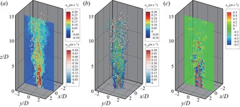
Instantaneous velocity field of bubble and liquid phase by FlowFit interpolation. (a) Streamwise velocity field and bubble tracking. (b) The  $Q$-criterion (
 $= 250\,{\rm s}^{-2}$) coloured by streamwise velocity. (c) Streamwise acceleration field.

Figure 8 shows a plane view of the instantaneous velocity field of the liquid phase obtained by FlowFit and STB (see supplementary movie 2). The instantaneous bubble positions and colour-coded bubble velocity are overlapped. The instantaneous velocity distribution of the continuous phase near the nozzle shows more complex flow patterns compared with that of a single-phase round jet (Davies, Fisher & Barratt Reference Davies, Fisher and Barratt1963). At the same Reynolds number, a single-phase jet has a potential core from  $z/D$ of 0.0 to 4.0. In the potential core, the velocity is uniform. The complex velocity pattern in this region of the bubbly jet is attributed to the motion of the bubbles. Immediately after the jet ejects, there tends to be a high-velocity zone from the inlet nozzle to a distance corresponding to the potential core. From that point, the high-velocity region of the water appears with rapidly rising bubbles.
After  $z/D > 10$, the velocity of the water is decreased, and the bubble rising velocity tends to be constant, as shown in figure 8(a). Figure 8(b) demonstrates an instantaneous 3-D vorticity structure of the liquid phase with a
 $Q$-criterion value of 250 s
 $^{-2}$ and colour-coding based on the streamwise velocity. The structure of the vortex has a small ‘worm’ shape and is distributed in both the core and edge of the jet with no specific directionality. In regard to the jet length scale, the measurement area covers the region where the initial momentum is dominant (
 $z < L_m$), and the jet transitions to a plume (
 $L_m < z < 5L_m$) (Fisher et al. Reference Fisher, List, Koh, Imberger and Brooks1979; Hunt & Kaye Reference Hunt and Kaye2001). In the jet-like region (
 ${z/L_m < 1},\ {z/D < 3.4}$) of the bubbly jet, the vortex structure shows a very dense distribution. After the transition to a bubbly plume (
 $1 < z/L_m < 5$), it can be observed that the vortex structure is coarsely distributed and becoming smaller. The rise of a bubble creates a wake behind it and continuously generates turbulence.
The instantaneous streamwise acceleration field at the centre plane is shown in figure 8(c), which is very interesting. Sciacchitano, Leclaire & Schröder (Reference Sciacchitano, Leclaire and Schröder2021) compared existing data assimilation approaches. For the FlowFit data assimilation, the acceleration bias error typically attains values within  $2\,\%$ of the fluid acceleration. In the jet-like region, very large acceleration and deceleration alternately appear, which can be explained by the interaction of the air bubbles and water flow. The bubble velocity is much higher than that of the water flow, and the water ahead of the bubbles decelerates quickly, while the water behind bubbles accelerates rapidly. The instantaneous acceleration field clearly distinguishes the strong ejection of the two-phase jet in the jet-like region, the transition region and the plume-like region far downstream. As air bubbles rise, the relative distance between the acceleration and deceleration regions increases, the acceleration magnitude decreases and the spatial distribution becomes coarse.
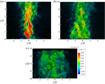
Figure 9 shows the instantaneous velocity vector field of the liquid phase at the centre plane ( $x/D = 0$). The instantaneous velocity vector field generally looks like a jet passing through porous media. As the bubbles rise, the water behind a bubble should follow it like added mass. Theoretically, the velocity of the added mass is half of the bubble velocity. The water slows down when the air bubbles leave the measurement plane.
Instantaneous velocity vector fields of liquid phase with heights in centre plane at  $x/D = 0$: (a)
 $0 < z/D < 5$, (b)
 $5 < z/D < 10$ and (c)
 $10 < z/D < 14$.

Figure 9(a) shows the instantaneous velocity vector field of the water in the jet-like region ( $z < L_m$) of the bubbly jet. In the case of a single-phase round jet, the potential core region appears from the nozzle exit to
 $z/D = 4$, and the velocity in the potential core is uniform. In this experiment, a high-velocity region with comparable jet exit velocity (
 ${>}0.3$ m s
 $^{-1}$) was observed at
 $0 < z/D < 4$. However, the water velocity is not uniform, and the fluid lump moves in a zigzag pattern and follows the bubbles.
Figure 9(b) shows the instantaneous water velocity vector field in the transition region. It can be observed that the velocity of the water decreases downstream of the jet, and the jet width is widening. High speed fluid lumps are observed in the centre of the bubbly jet. Figure 9(c) shows the instantaneous velocity vector field in the plume region. Water flow tends to be relatively uniform without a significant difference in the magnitude of the velocity, but there are footprints of air bubble motions. A statistical analysis is discussed in the next section.
3.2. Mean velocity profile and slip velocity
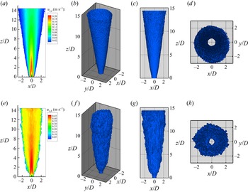
Figure 10 shows the ensemble-averaged velocity field at the centre plane ( $x$–
 $z$ plane) and 3-D iso-surface contours of the streamwise velocity of the liquid and gas phases. Iso-surfaces were extracted from the ensemble-averaged velocity fields by setting the threshold velocity as 0.02 m s
 $^{-1}$ for the liquid phase and 0.05 m s
 $^{-1}$ for bubbles. The maximum rising velocity of a bubble was more than twice compared to the maximum velocity of the water.
Ensemble-averaged velocity fields and iso-surfaces of streamwise velocity of (a–d) liquid phase and (e–h) bubble. (a,e) Centre plane, (b,f) 3-D view, (c,g) front view and (d,h) top view.

Figure 10(a) shows the contour of the ensemble-averaged velocity field of the water phase in the centre plane. Due to the locations of the needles in the bubble generator, the jet velocity profile at the nozzle exit resembles a coaxial circular jet (van Hout et al. Reference van Hout, Murugan, Mitra and Cukurel2021).
Very near the nozzle ( $z/D < 1$), primary and secondary potential cores were developed. The bubbles divided the exit flow with the inner and outer shear layers. We call this area the initial merging zone. In the region of
 $1 < z/D < 2$, the primary and secondary potential cores merge, and this zone is called the intermediate zone. After
 $z/D > 2$, a coaxial circular jet merges to form a fully merged zone. From this area, a typical bubbly flow configuration is generated. In a typical bubbly flow, there is a transition from the zone of flow establishment (ZFE) to the zone of established flow (ZEF). The ZFE tends to have a high velocity at the centre of the jet to a distance corresponding to the potential core. Consequently, the high-velocity region of the water is dispersed in space, forming a ZEF.
Figure 10(b–d) shows iso-surfaces of the streamwise velocity of the liquid phase. Iso-surfaces are presented based on  $10\,\%$ of the maximum velocity (0.02 m s
 $^{-1}$) and show the kinematic characteristics of the continuous-phase flow in the bubbly jet. Figure 10(b,c) shows that the water flow is statistically stable. The clear cone shape of the velocity iso-surface means the water spreads linearly downstream above
 $z/D > 2$.
Figure 10(e) shows the ensemble-averaged velocity field of the bubbles in the centre plane. Compared with the water velocity (figure 10a), the rising velocity of the bubbles is much higher. Due to the shape of the bubble generator, bubbles ejected by the needles merge at  $z/D = 1$ and then develop into a typical bubbly jet. Up to
 $z/D = 4$, the high bubble velocity in the core region (
 $-0.5 < x/D < 0.5$) is uniform and straight.
Downstream of  $z/D = 4$, the bubble velocity along the centreline decreases monotonically. In the plume region, the bubble velocity becomes the terminal velocity and tends to be uniform in a horizontal cross-sectional area. Figure 10( f–h) shows the iso-surfaces of the bubble rise velocity taken at
 $10\,\%$ of the maximum rising velocity (0.05 m s
 $^{-1}$). As shown in figures 10( f) and 10(g), bubbles spread more rapidly in the jet-like region of the bubbly jet (
 $z < L_m$) and then spread linearly along the downstream direction with lower growth rate compared with that of the liquid phase.
Figures 10(d) and 10(h) show top views of the iso-surface of the streamwise velocity of the water and bubbles. As mentioned in § 2.1, four distributed suction tubes were installed to spread the bubble plume as straight as possible during the experiment. Figure 10(d) shows the iso-surface of water velocity. This figure confirms that the ensemble-averaged velocity field of the continuous phase is axisymmetric. The threshold of the iso-surface is 0.02 m s $^{-1}$, so the centre hole in figure 10(d) means the velocity is always higher than 0.02 m s
 $^{-1}$. Figure 10(h) shows that the mean bubble velocity is also axisymmetric like the water flow. The hole in figure 10(h) denotes that the bubble velocity in the centre region is always higher than 0.05 m s
 $^{-1}$. So far, the bubbly jet or plume has been assumed to have an axisymmetric flow configuration. This assumption was verified through the 3-D measurements in this experiment.
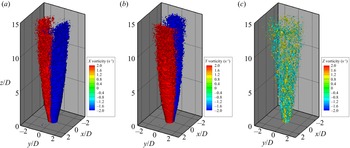
One more great advantage of 3-D velocity field measurement is resolving the 3-D vorticity field using velocity derivatives. Figure 11 shows the ensemble-averaged vorticity fields of the liquid phase. Since the flow is axisymmetric, the  $x$- and
 $y$-component vorticities obtained with the same threshold (2 Hz) have the same configurations as shown in figures 11(a) and 11(b). In the jet-like region (
 $z/L_m < 1$), the positive and negative iso-surfaces of
 $x$ and
 $y$ components of vorticity are attached along
 $y = 0$ and
 $x = 0$ planes. In the transition to plume region (
 $z/L_m > 1$), discrete contours appear and irregular boundaries are shown in both
 $x = 0$ and
 $y = 0$ planes. In the plume region, the positive and negative iso-surfaces depart from each other because vorticity magnitudes of
 $x$ and
 $y$ components are weaker than the threshold.
Ensemble-averaged vorticity field of liquid phase: (a)  $x$-component vorticity, (b)
 $y$-component vorticity and (c)
 $z$-component vorticity.

Figure 11(c) shows the 3-D ensemble-averaged streamwise vorticity ( $z$-component vorticity) iso-surfaces extracted at
 $+1$ Hz (yellow) and
 $-1$ Hz (cyan). Surprisingly, the ensemble (accumulated)
 $z$-vorticity distribution using 36 300 realizations shows a discrete feature unlike
 $x$ and
 $y$ components of vorticity. This result can be explained in that the streamwise vorticity structures are generated by bubble motions and the void fraction in this experiment is very low (
 $0.12\,\%$). Counter-rotating vortex pairs and streaky structures of the streamwise vorticity are clearly seen in the jet-like region. The ensemble-averaged
 $z$-vorticity structure collapses as it goes downstream. In the plume region, a random and intermittent distribution of the streamwise vortex structures is shown and it is induced by vortex breakdown. This is direct evidence of the energy cascading process of the turbulent eddies by bubbles.
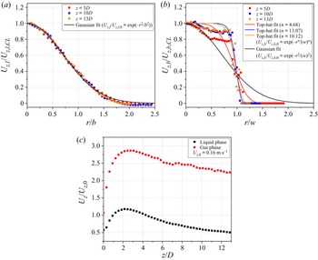
Figure 12 shows the streamwise velocity profiles of the liquid and gas phases at various  $z$ positions, which were used to analyse the mean flow characteristics of the turbulent bubbly jet along the radial direction. Using the phase-separation method, we plotted the mean streamwise velocity profiles of the continuous phase and dispersed phase. In classical frameworks of bubbly plumes, the mean flow of the continuous phase has a Gaussian distribution (Priestley & Ball Reference Priestley and Ball1955; Morton, Taylor & Turner Reference Morton, Taylor and Turner1956). A Gaussian velocity profile has been commonly used to describe the mean flow profile which is defined as follows:
 \begin{equation} U_{z,l} (r,z) = U_{z,l,CL}(z)\exp({-}r^2/b^2), \end{equation}
where  $U_{z,l}$ and
 $U_{z,l,CL}$ are the time-averaged streamwise velocities of the liquid phase and along the centreline, respectively,
 $r$ is the radial position and
 $b$ is the velocity half-width. The velocity half-width is given by the radial coordinate, where
 $U_{z,l}/U_{z,l,CL}=1/e$.
Streamwise velocity profiles normalized by the local centreline velocity and the initial jet velocity calculated from water flow rate ( $= 0.16$ m s
 $^{-1}$). (a) Radial distribution of the continuous phase. (b) Radial distribution of bubble velocity. (c) Centreline velocity along the heights.

Figure 12(a) shows the radial profiles of the streamwise velocity in the liquid phase at different heights from the jet outlet. The mean velocity was normalized by the streamwise centreline velocity. The radial position  $r$ was normalized to the velocity radius
 $b$ obtained from the Gaussian profiles. The velocity profiles are mostly consistent with Gaussian distributions and have self-similarity. A discrepancy from the Gaussian profile occurs at more than
 $r/b = 1.5$, which is probably caused by a large recirculation inside the tank.
The velocity profile of the dispersed phase is more similar to a top-hat profile, which is different from the Gaussian distribution. As shown in figure 12(b), the top-hat distribution must be considered to evaluate the rising velocity of a bubble. Like the Gaussian velocity profile of the liquid phase, the velocity profile of bubbles is defined as follows:
 \begin{equation} U_{z,b} (r,z) = U_{z,b,CL}(z)\exp({-}r^n/w^n), \end{equation}
where  $n$ is a parameter that adjusts the flatness of the centre of the profile and
 $w$ is the bubble half-width. As a result, the bubble velocity reaches the terminal velocity as it goes downstream, causing the bubble to move at a constant velocity. Even if the bubble reaches terminal velocity, it is riding on the continuous-phase velocity field. Due to this, the data are slightly off the top-hat fitting line. Table 2 shows the adjusted
 $R^{2}$ value of the Gaussian fitting for liquid/gas phases and top-hat fitting for the gas phase. The bubble is raised by buoyancy and eventually reaches terminal velocity if the diameter of the bubble is constant. The bubble generator produced fairly monodispersed bubbles with a diameter of
 $1.727 \pm 0.179$ mm (Seo & Kim Reference Seo and Kim2021). The bubble velocity distribution is well fitted with a Gaussian distribution in the jet core (
 $r/w < 0.5$), but the mean bubble velocity in the jet edge coincides with a top-hat profile.
Adjusted  $R^{2}$ value of Gaussian and top-hat fitting in velocity profiles.

The characteristics of the ZEF and ZFE of the bubbly jet were observed with the variation of the streamwise velocity along the centreline, as shown in figure 12(c) (van Hout et al. Reference van Hout, Murugan, Mitra and Cukurel2021). The streamwise velocity was normalized by the initial velocity of the nozzle outlet. The initial velocity of the water,  $U_{z,0}$, was calculated from the water flow rate (3 l min
 $^{-1}$) based on the top-hat profile assumption at the outlet of the bubble generator. In the jet-like region, the buoyancy accelerates the centreline streamwise velocity. The bubbles accelerate the plume and make it have jet-like behaviour. Based on the bubbly jet analysis, ZFE transitions to ZEF when acceleration is finished, which means the collapse of the potential core of the jet (Henderson-Sellers Reference Henderson-Sellers1983). The measured instantaneous velocity field (figure 9a) in the jet-like region confirms this behaviour.
Figure 12(c) clearly shows that there is a velocity peak around  $z/D = 3.4$ (
 $z/L_m = 1.0$). This transition is consistent with the theoretical description of Morton (Reference Morton1959) of a balance between the momentum flux and buoyancy flux around
 $L_m$. After the collapse of the potential core, the bubbly jet follows the transition area (
 $1 < z/L_m < 5$) from the jet to the plume (Fisher et al. Reference Fisher, List, Koh, Imberger and Brooks1979; Hunt & Kaye Reference Hunt and Kaye2001).
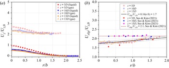
Figure 13 compares the radial distributions of the ensemble-averaged streamwise velocity at various vertical positions for liquid- and gas-phase flows. They were normalized by the initial velocity of the bubbly jet and used to evaluate slip velocity along the radial direction with different heights. In figure 13(a), the radial profiles of the streamwise velocity of liquid and gas are indicated by filled and open symbols, respectively. Interestingly, the liquid velocity decreases downstream, while the bubble velocity remains rather constant along the streamwise direction in the intermediate and plume regions.
(a) Comparison of normalized streamwise velocity between liquid and gas phase and (b) slip ratio variation in radial directions.

Figure 13(b) shows the slip ratio profile of the air bubbles at different heights. Slip velocity in gas–liquid flow is defined as the difference of the velocity between the gas phase and liquid phase. The slip velocity  $U_{slip}$ is the relative velocity between a bubble and the liquid phase:
 \begin{equation} U_{slip} (r,z) = U_{z,b}(r,z)-U_{z,l}(r,z), \end{equation}
where  $U_{z,b}$ is a bubble's rising velocity (Seo & Kim Reference Seo and Kim2021; Seo et al. Reference Seo, Marjanovic, Balachandar and Kim2022). In figure 13(b), the slip velocity and radial direction are normalized by the initial water jet velocity and the velocity radius. The slip ratio of the bubble linearly increases in the radial direction but remains constant regardless of heights. The slip ratio varies from 1.75 to 2.05, and the lowest slip velocity is observed at the centre. The acquired slip ratio has a relationship with the radial direction fitted as follows:
 \begin{equation} U_{slip}/U_{z,0} = 0.16(r/b)+1.7. \end{equation}
The black solid and dashed lines shown in figure 13(b) represent the linear fitting results and standard deviation of the sampled slip velocity data, respectively. The increasing rate of the slip velocity along the radial direction is attributed to the Gaussian profile of the liquid and the constant terminal velocity of the bubble. According to a previous 2-D measurement study (Seo & Kim Reference Seo and Kim2021), the slip velocity is represented by a red dashed line without including the data at  $z/D = 5$. The 2-D measurements showed that the slip ratio remained constant along the radial direction in the intermediate and plume regions. Most previous studies also argued that bubbly plumes consisting of homogeneously dispersed bubbles have a constant slip velocity (Ditmars & Cederwall Reference Ditmars and Cederwall1975; Brevik Reference Brevik1977). However, our 3-D measurement of the bubble velocity resulted in a linear increase in slip velocity along the radial direction for a given condition.
The relative velocity magnitude between water and bubbles (slip velocity) can affect to the flow physics in a turbulent bubbly jet. In this study, the water jet velocity at the nozzle exit was about 0.3 m s $^{-1}$ (
 $Re = 3172$) which is comparable to the bubble velocity (0.28 m s
 $^{-1}$; see table 1). The water jet velocity along the centreline quickly decreased to 0.16 m s
 $^{-1}$ while the bubble velocity was about 0.44 m s
 $^{-1}$ (
 $U_{slip} = 1.75U_{z,0}$) at
 $z/D = 5.0$ as shown in figure 13(b). In order to provide the water jet velocity that can be comparable to the bubble velocity needs a water jet two to three times faster than in this study (
 $6000 < Re < 9000$). Wang & Law (Reference Wang and Law2002) and Sun & Faeth (Reference Sun and Faeth1986) conducted measurements of a buoyant jet with
 $Re = 6000$ and 8740 in the asymptotic self-similar region of the jet. The difference in flow physics between our result and high-Reynolds-number results is the change of position where the jet-like structure becomes the plume-like structure. The influence of slip velocity in a two-phase bubbly jet is thoroughly discussed in our recent publication (Seo et al. Reference Seo, Marjanovic, Balachandar and Kim2022).
In terms of the integral plume modelling, the time-averaged dynamics of the air–water bubble plumes is dependent on the length scale  $D_b$, which can be derived from the governing equation of the two-fluid numerical model (Bombardelli et al. Reference Bombardelli, Buscaglia, Rehmann, Rincón and García2007):
 \begin{equation} D_{b} = gQ_{b}/4{\rm \pi}\alpha^2U_{slip}^3, \end{equation}
where  $g = 9.81$ m s
 $^{-2}$ is gravity,
 $Q_b$ is the volumetric flow rate of a bubble,
 $\alpha = 0.083$ is the plume entrainment coefficient and
 $U_{slip}$ is the slip velocity. In this study,
 $U_{slip}$ was the centre slip velocity of 0.28 m s
 $^{-1}$ (
 $U_{slip} = 1.75U_{z,0}$) from figure 13(b). Previous studies used the slip velocity calculated from the correlation depending on the bubble diameter (Clift et al. Reference Clift, Grace and Weber1978; Motarjemi & Jameson Reference Motarjemi and Jameson1978). Length scale
 $D_b$ was calculated as 8.3 mm in the present study.
The length scale  $D_b$ separates
 $z$ above the source into two characteristic regions in a classic bubbly plume. For a non-dimensional source height
 $z/D_b < 5$, the bubbly plume is in the adjustment stage and depends on source conditions (e.g. diameter of the source and geometry). For
 $z/D_b > 5$, the plume is in an asymptotic region, where the source condition is ignored, and all normalized plume properties behave in the same way (Bombardelli et al. Reference Bombardelli, Buscaglia, Rehmann, Rincón and García2007). The jet-like region is apparent at
 $z/D_b < 5$, but our jet-like flow does not behave similarly to the results of Bombardelli et al. (Reference Bombardelli, Buscaglia, Rehmann, Rincón and García2007) due to different source geometry and condition.
In this study,  $L_m$ length scale was used to compare with other studies in the plume-like region. It seems necessary to develop a length scale that follows our experimental regime. As shown in figure 14, the appropriate length scale for this study is newly defined as
 $(z-L_m)/D_b$. The existing pure bubble plume was defined as a plume-like region in the
 $z/D_b > 5$ region, but the jet used in this study exhibited a plume-like behaviour from
 $z/D_b > 13\ (= (z-L_m)/D_b) > 5$).
Schematic of length scale used in this study.

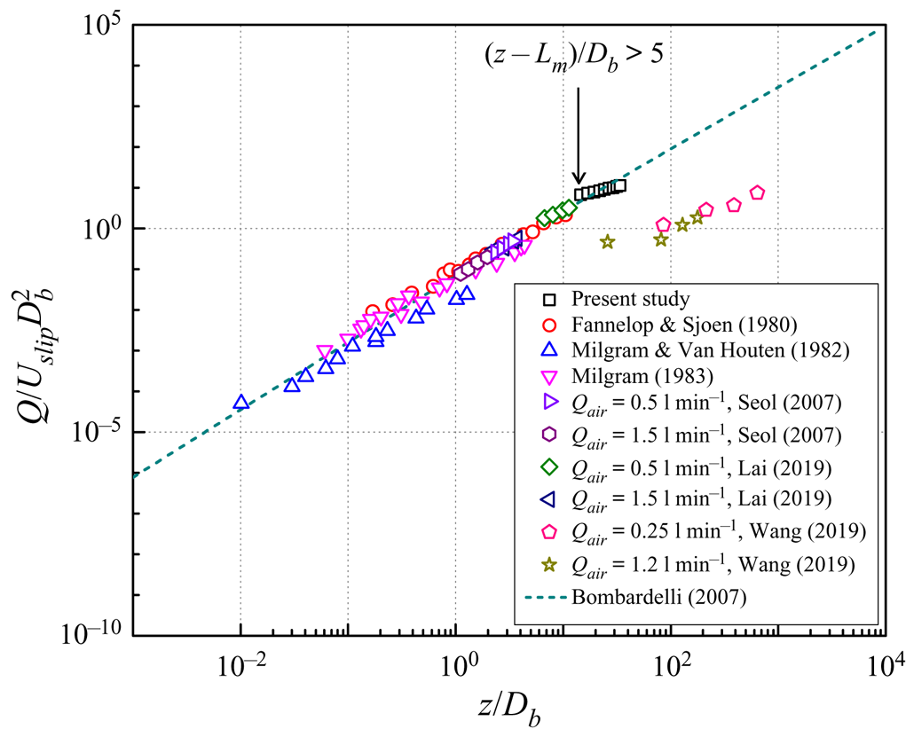
To evaluate the integral behaviour of the turbulent bubbly plume, a general-purpose scaling rule was applied to normalize the mean flow characteristics of the bubbly plumes with available literature data (Fannelop & Sjoen Reference Fannelop and Sjoen1980; Milgram & Van Houten Reference Milgram and Van Houten1982; Milgram Reference Milgram1983; Seol et al. Reference Seol, Bhaumik, Bergmann and Socolofsky2007; Lai & Socolofsky Reference Lai and Socolofsky2019; Wang et al. Reference Wang, Lai and Socolofsky2019). In this study, the comparison of jet-like regions ( $(z-L_m )/D_b < 5$) is not considered.
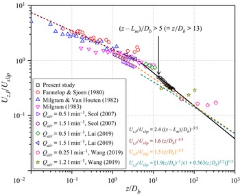
Figure 15 shows the scaling of the centreline velocity of the liquid phase with  $z$ above the source. Here
 $U_{z,l}$ and
 $z$ are scaled by
 $U_{slip}$ and
 $D_b$, respectively. It is well demonstrated that the centreline velocity changed with the height along the plume downstream in a classic single-phase plume. Fisher et al. (Reference Fisher, List, Koh, Imberger and Brooks1979) showed that the centreline velocity scaled to
 $z^{-1/3}$ in a continuous-phase plume. In addition, Bombardelli et al. (Reference Bombardelli, Buscaglia, Rehmann, Rincón and García2007) proposed an integral model of a classic bubbly plume for
 $z/D_b < 5$ that was scaled as follows and is shown with a red dashed line:
 \begin{equation} U_{z,l}/U_{slip} \sim (z/D_b)^{{-}1/3}. \end{equation}
Plume core velocity normalized by the slip velocity along the heights.

This scaling is typically valid in classic bubbly plumes (Lemckert & Imberger Reference Lemckert and Imberger1993). Data except those from Wang et al. (Reference Wang, Lai and Socolofsky2019) are not exactly accumulated but are close to this scaling. Bombardelli et al. (Reference Bombardelli, Buscaglia, Rehmann, Rincón and García2007) obtained an analytical solution for the centreline velocity at  $z/D_b \gt \gt 1$ in a classic integral bubbly plume model, which is shown with an orange dashed line:
 \begin{equation} U_{z,l}/U_{slip} \sim (z/D_b)^{{-}1/2}. \end{equation}
Bombardelli et al. (Reference Bombardelli, Buscaglia, Rehmann, Rincón and García2007) also used numerous simulations to obtain asymptotic equations for  $z/D_b > 5$, which are shown with a green dashed line:
 \begin{equation} U_{z,l}/U_{slip} \sim[(1.9(z/D_b)^{{-}1})/(1+0.563(z/D_b)^{1/2})]^{1/3}. \end{equation}
We found that all available literature data typically track each solution, but there is a clear difference between the measured data and the solution of the integral model. The scattered data deviated from the classic plume model, and asymptotic solution lines show that for the reported integral model, it is difficult to predict the plume velocity of the turbulent bubbly jet flow. This happens because the plume velocity is calculated indirectly from the volume and momentum flux that were resolved in the previous integral model, indicating that the dilute bubbly mixed jet does not follow the physics of a classic bubbly plume. Thus, the classic integral theory for a bubbly plume cannot predict the exact evolution of the plume core velocity in a dilute bubbly mixed jet.
Our data show a different physical characteristic around  $(z-L_m)/D_b = 5$ as shown in figure 15. After the jet-like region, the liquid phase has plume-like behaviour and acts differently from previously reported scaling physics. In this study, we found that the plume core velocity is scaled to
 $z^{-3/5}$ in a continuous phase of the plume, as shown with a black solid line:
 \begin{equation} U_{z,l}/U_{slip} \sim ((z-L_m)/D_b)^{{-}3/5}. \end{equation}
This centreline velocity along the plume height provides the volume flux. This is discussed in § 3.4.
3.3. Plume width and spreading characteristics
Next, the population of bubbles was correlated with the liquid-phase flow of the bubbly jet. Figure 16 shows the distribution of the accumulated bubble population with different heights during 100 time steps. Dashed red circles in figure 16(a–c) represent the outlet periphery of the bubble generator ( $r/D = 0.5$). The solid black circle in figure 16(d) represents the maximum distribution area of the bubble population to calculate the volumetric air void fraction. Figure 16(a–c) shows top views of the captured air bubbles at
 $z = 5D$,
 $10D$ and
 $13D$, respectively. Downstream of the bubbly jet, little air bubbles are observed in the centre. In previous studies, cross-sectional air void fractions were calculated in 2-D planes (Wang et al. Reference Wang, Lai and Socolofsky2019; Li et al. Reference Li, Wang, Wu and DiMarco2020). But with those methods, it is intrinsically impossible to obtain accurate volumetric air void fractions because they fail to capture bubbles that are out of the 2-D plane which causes large errors when calculating the time-averaged results.
Distribution of bubble population. Top view (a) at  $z = 5D$, (b) at
 $z = 10D$, (c) at
 $z = 13D$ and (d) total bubble population. (e) Front view of accumulated bubbles of 100 time series at
 $y/D = 0$. Dashed red circle in (a–c) represents outlet of bubble generator,
 $r/D = 0.5$. Solid black circle in (d) represents maximum distribution area to obtain bubble population.

The cross-sectional void fraction is the projected area void fraction that accumulates vertically on the bubble image plane, which differs from the volumetric void fraction (defined as the volume ratio of the gas phase in the 3-D liquid phase). The actual volumetric or local void fraction could be several times smaller than that of the 2-D measurement. In this study, the exact control volume for the liquid phase can be obtained because we know the 3-D distribution of the bubble locations and the maximum volume where bubbles are distributed.
Figure 16(d) shows a top view of the maximum distribution area of the bubble population with a radius of  $r/D = 1.9$. Combined with
 $r/D = 0.5$, which is the outlet radius of the nozzle, the volume of the liquid phase can be obtained from a cut circular cone shape (565 560 mm
 $^{3}$). Using a total of 36 300 time steps, the average number of bubbles in this fluid volume at an instance was 259. Assuming spherical bubbles have a diameter of 1.7 mm (
 $d_{avg,b}$), the total volume of the bubbles can be obtained as follows:
 \begin{equation} \tfrac{4}{3}{\rm \pi}(d_{avg,b}/2)^3 \times n = 666\,{\rm mm}^3. \end{equation}
The average volumetric air void fraction in the control volume is calculated as  $0.12\,\%$. This value is one order less compared with the inlet void fraction,
 $1.0\,\%$. This can be explained in that the bubbles are widely spread in the control volume. The advantage of the present 3-D simultaneous LPT measurement is that it is possible to determine the 3-D positions of the dispersed phase and the exact number of bubbles. The proposed method can provide both cross-sectional and volumetric-averaged void fractions. Volumetric void fraction is the most important physical quantity and a key parameter in two-phase flow for design and performance evaluations of two-phase systems and devices. If we have enough data, we can quantify the void fraction distribution along the height. With the 2-D void fraction measurement methods such as conductance probe and 2-D imaging approaches, evaluation of void fraction in a horizontal slice is very difficult because bubbles pass through the laser light sheet very quickly and the number of probes is limited. Therefore, definition of void fraction is mostly decided by inlet conditions such as flow rates of two fluids. In real flow configurations, bubbles disperse into the continuous phase. So the measurement of a volume void fraction in a flow system is important to understand bubbly flows.
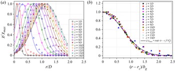
Figure 17 shows the radial distribution of the air void fraction and self-similarity of dispersed field concentration. The air void fraction is expressed by the number of bubbles  $\chi$ in each radial position and normalized by the maximum number of bubbles
 $\chi _{max}$ occurring at each height. As shown in figure 17(a), most bubbles are distributed in the form of shifted Gaussian profiles along the radial directions. When the flow goes downstream, the centre position of each Gaussian profile deviates from the jet core region. Nevertheless, the population of bubbles also maintains its self-similarity, as shown in figure 17(b). Previous studies of a bubbly jet and plume reported that air bubbles were distributed in a Gaussian profile with peaks along the centreline of the flow (Sun & Faeth Reference Sun and Faeth1986; Seol et al. Reference Seol, Bhaumik, Bergmann and Socolofsky2007; Wang et al. Reference Wang, Lai and Socolofsky2019). Note that the study of Wang et al. (Reference Wang, Lai and Socolofsky2019) was for weak bubble plumes, which they defined as plumes that lacked entrainment or a coherent continuous-phase velocity field. Hence, their data are completely different from those for a bubbly jet near the transition to plume-dominated flow. One of the main discrepancies between our study and previous studies is the inlet void fraction. The inlet void fraction was reported as 2.4 %–9.1 % at the outlet of the bubbly jet (Sun & Faeth Reference Sun and Faeth1986) and 3 % near the bottom of the plume (Seol et al. Reference Seol, Bhaumik, Bergmann and Socolofsky2007). However, our case shows an inlet void fraction based on mass that is less than
 $1\,\%$. The volumetric void fraction in the bubbly jet was even
 $0.12\,\%$, as shown in figure 16. In previous studies, highly packed bubbles resulted in redistribution of the bubbles in the flow and formed a distribution similar to that of a Gaussian profile. However, the present dilute bubbly mixed jets show shifted Gaussian profiles of air bubbles concentrated in the velocity radius region where a high-shear region is formed. This phenomenon is observed in two-phase pipe and channel flows and is described as shear-induced meandering (Aliyu et al. Reference Aliyu, Almabrok, Baba, Archibong, Lao, Yeung and Kim2017).
Radial distribution of air void fraction. (a) Shifted Gaussian function along the radial direction. (b) Self-similarity with a Gaussian distribution function.

To evaluate the evolution of the bubble population with almost the same framework of the liquid phase as (3.1), the radial position with a Gaussian centre  $r_c$ was normalized by the bubble radius
 $b_g$, which is defined as follows:
 \begin{equation} \chi/\chi_{max} = \exp(-(r-r_c)^2/b_g^2). \end{equation}
From figures 12(a) and 17(b), the velocity and bubble radius of the bubbly jet can be determined from Gaussian profiles at different heights above the source.
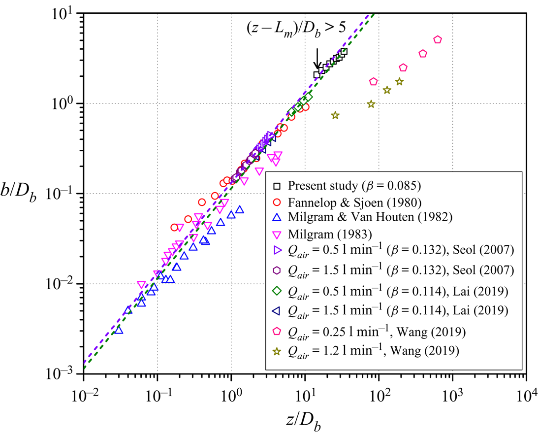
Figure 18 shows the scaling of the velocity radius  $b$ with the heights. Here
 $b$ and
 $z$ are normalized by plume length scale
 $D_b$. At
 $z/D_b > 13$ (
 $z-L_m/D_b > 5$), the bubbly jet acts as a coherent single-phase plume with classical linear spreading dynamics (e.g.
 $b = \beta z$). Parameter
 $\beta$ is the spreading rate, and for a classical bubbly plume, it is similar to that of a single-phase circular plume (Ditmars & Cederwall Reference Ditmars and Cederwall1975), depending on the linear spreading behaviour:
 \begin{equation} {\rm d} b/{\rm d} z = \beta, \end{equation}
where  $\beta \approx 0.1$ (Fisher et al. Reference Fisher, List, Koh, Imberger and Brooks1979).
Variation of velocity half-width  $b$ along the height.

As references, figure 18 shows linear spreading relationships at  $b/z = 0.114$ (green dashed line; Lai & Socolofsky Reference Lai and Socolofsky2019) and 0.132 (purple dashed line; Seol et al. Reference Seol, Bhaumik, Bergmann and Socolofsky2007). The linear spreading tracks the literature data relatively well in the range of four orders of magnitude in
 $z/D_b$. The physical mechanism of the linear spreading means entrainment is constant (Morton et al. Reference Morton, Taylor and Turner1956; Crapper Reference Crapper1977; Lai et al. Reference Lai, Chan, Law and Adams2016). Typically, the linear spreading rate is observed by many research groups at the region of
 $z/D_b < 1$ of the bubbly plume. Our data matched well those suggested by previous reports and
 $\beta$ values in the plume region.
The measured spreading rate,  $\beta = 0.085$, is lower than that of the previously reported bubbly plumes (
 $\beta = 0.1$), but slightly higher than that of turbulent round jets (
 $\beta = 0.080$) (Davies et al. Reference Davies, Fisher and Barratt1963). A reference line for single-phase round plumes with
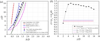
 $\beta = 0.1$ is marked as the green dashed line in figure 19(a). This behaviour can be explained in that the present dilute bubbly jet has a higher continuous-phase velocity in the jet region, which yields higher shear at the plume edge. The absolute
 $b$ value is larger than those in previous studies, which can be larger with lower centreline velocity
 $U_{z,l}$. The variation of the
 $b$ values is very comparable with the
 $U_{z,l}$ data (see figure 15).
Comparison of (a) half-width with the 2-D particle image velocimetry results and (b) plume spreading ratio between liquid and gas phase.

When buoyancy force is applied to the air bubbles, the leading air bubbles more easily escape from the turbulent wake and form a wide plume width. This behaviour of a bubble enhances the lateral transport of the kinetic energy in the plume, increasing the plume width and decreasing the plume velocity. The water velocity decreases due to the lateral increase of the plume because of the shear entrainment occurring at edge of the plume. Figure 19(a) compares the evolution of the velocity radius  $b$ and the bubble population radius
 $b_g$ with heights. Interestingly, the Gaussian centre position
 $r_c$ and
 $b$ evolve similarly along the entire measurement area.
In the jet-like region,  $r_c$ and
 $b$ match the configuration as shown in figure 10. Subsequently, the bubbly jet radius is linearly proportional to the height. From the transition to the plume-like region,
 $b$ and
 $b_g$ maintain linear spreading to the end of the measurement height. Modulation of the bubble population can be affected by the high-shear region of a dilute bubbly mixed jet (Fraga et al. Reference Fraga, Stoesser, Lai and Socolofsky2016; Seo & Kim Reference Seo and Kim2021).
In a bubbly plume, the spreading ratio is defined as  $\lambda = (r_c+b_g/b)$. Ratio
 $\lambda$ is an important parameter in the governing equation of the integral model and is typically considered to be less than 1 (Socolofsky, Bhaumik & Seol Reference Socolofsky, Bhaumik and Seol2008). The measured spreading ratio rapidly increases to
 $z/D < 4$ and then slowly decreases, as shown in figure 19(b). For the previously reported
 $b_g$, the
 $\sqrt {2}$ appearing in
 $\lambda$ accounts for the difference between the top-hat and Gaussian profiles of the integral plume models (Lai & Socolofsky Reference Lai and Socolofsky2019). Parameter
 $b_g$ is interpreted as a top-hat radius, so the factor of
 $\sqrt {2}$ is used on
 $b$ when calculating the spread ratio
 $\lambda$. The constant-
 $\lambda$ assumption is no longer validated in the present experimental data because the present bubbly jet has a higher continuous-phase velocity in the jet region, which yields higher shear at the plume edge.
3.4. Unified scaling of various bubbly flows
The volume flux of the continuous phase can be calculated by integrating the Gaussian profile of the liquid velocity. The volume flux of the plume is defined as follows:
 \begin{equation} Q(z) = \int_{0}^{\infty}2{\rm \pi} r (1-\chi(z,r))U_{z,l}(z,r)\,{\rm d} r, \end{equation}
where  $\chi$ is the air void fraction. This equation means that the integral properties of the plume are axisymmetric, as shown in figure 12(a,b). It is also approximated by
 ${(1-\chi ) \approx 1}$ via a dilute-plume assumption. From the Gaussian profile assumption, we can derive the volume flux as follows:
 \begin{equation} Q(z) = 2{\rm \pi}\int_{0}^{\infty}U_{z,l,CL}\exp({-}r^2/b^2)r\,{\rm d} r = {\rm \pi}U_{z,l,CL}b^2. \end{equation}
We derived a scaling that combines the classic bubble plume with our study. Using a non-dimensional analysis, we compared the behaviour of the bubbly jet with classic plumes. Figure 20 shows the non-dimensional volume flux versus height in a bubble plume. The non-dimensional volume flux is normalized to  $D_b$ and
 $U_{slip}$ as
 $Q/(D_bU_{slip}^2)$. As a result, the integral model still allows the intrinsic properties of the flux in the plume, although the individual parameters of the plume (i.e. the plume velocity and width) may differ.
Non-dimensional volume flux versus height in bubbly plumes.

For classic bubbly plumes, we adopted an asymptotic solution from Bombardelli et al. (Reference Bombardelli, Buscaglia, Rehmann, Rincón and García2007) for  $U_{z,l}$ and
 $b$. Integral models are effective in predicting the volume flux of bubbly plumes. The dashed line in figure 20 represents the volume flux derived from asymptotic solutions with Gaussian velocity profiles and the linear spreading hypothesis:
 \begin{equation} Q/D_bU_{slip}^2 = 2{\rm \pi}\beta^2[(1.9(z/D_b)^{5})/(1+0.563(z/D_b)^{1/2})]^{1/3}, \end{equation}
where  $\beta = 0.1$ for linear spreading in a single-phase plume. This equation matches well with our data in the plume region. The increase in volume flux is the result of the inflow of ambient water into the bubbly plume. Ambient water flowing into the plume is driven by an internal velocity component perpendicular to the direction of the plume rise (see figure 9).
The entrainment hypothesis states that the increase in liquid volume is due to shear entrainment of ambient liquid at the edge of the jet or plume with an entrainment velocity  $U_e$, which is proportional to the centreline velocity multiplied by the entrainment coefficient
 $\alpha$ (
 $U_e = \alpha U_{z,l,CL}$) (Turner Reference Turner1986). Because classic bubble plumes spread linearly in a way similar to that of single-phase jets and plumes, the entrainment hypothesis of single-phase jets and plumes is adopted in many integrated models of classic bubbly plumes (Asaeda & Imberger Reference Asaeda and Imberger1993; Bombardelli et al. Reference Bombardelli, Buscaglia, Rehmann, Rincón and García2007; Socolofsky et al. Reference Socolofsky, Bhaumik and Seol2008). From Gaussian profile assumptions, the conservation of volume flux equation is derived as follows:
 \begin{equation} {\rm d}({\rm \pi} U_{z,l,CL}b^2)/{\rm d} z = 2{\rm \pi} \alpha U_{z,l,CL}b. \end{equation}
From the measured data, the effective entrainment coefficient can be calculated by the relationship between the maximum mean velocity of the fluid phase and the volume flux into the plume. This equation can be expressed as volume flux (Milgram Reference Milgram1983):
 \begin{equation} {\rm d} Q/{\rm d} z = 2{\rm \pi} \alpha U_{z,l,CL}b. \end{equation}
The gradient of the volume flux was determined by eliminating the noise that can be obtained by fitting the volume flux data in figure 20 to a linear curve.
The entrainment coefficient is determined using the obtained gradient of the volume flux and centreline velocity of the continuous phase. Figure 21 shows the relationship of the entrainment coefficient with the normalized height and normalized parameter (Seol et al. Reference Seol, Bhaumik, Bergmann and Socolofsky2007). As shown in figure 21(a), the scaling is useful for evaluating the relationship between the entrainment coefficient and the height above the source over the entire range of available bubble plume data. The entrainment coefficient of the single-phase plume is 0.083. As the bubbly jet goes downstream, the entrainment coefficient continues to decrease, placing it in the range 0.05–0.04. In this regime, the plume behaves like a simple plume in the measurement domain, and non-constant entrainment coefficient indicates that the plume is not strictly self-similar.
Relationship of entrainment coefficient with (a) normalized height and (b) normalized parameter.

Seol et al. (Reference Seol, Bhaumik, Bergmann and Socolofsky2007) proposed a dimensionless slip velocity as a scaling factor to provide a functional relationship between the entrainment coefficient and other local independent variables of a bubble plume. The dimensionless slip velocity can be expressed as  $U_{slip}/(B_0/z)^{1/3}$, where
 $B_0$ is the initial buoyancy flux. This parameter is the ratio of the slip velocity to the characteristic liquid velocity
 $(B_0/z)^{1/3}$. The entrainment coefficients based on this scaling factor provide the following functional relationship:
 \begin{equation} \alpha = 0.18 \exp({-}1.7U_{slip}/(B_0/z)^{1/3})+0.04. \end{equation}
Figure 21(b) shows the relationship between the entrainment coefficient and the dimensionless parameter with available literature data (Fannelop & Sjoen Reference Fannelop and Sjoen1980; Milgram & Van Houten Reference Milgram and Van Houten1982; Milgram Reference Milgram1983; Hugi Reference Hugi1993; Seol et al. Reference Seol, Bhaumik, Bergmann and Socolofsky2007; Wang et al. Reference Wang, Lai and Socolofsky2019). The data indicate a dependence of the entrainment coefficient on height from the source, initial buoyancy flux and slip velocity. The entrainment coefficient decreases as the plume rises. This scaling shows that the slip velocity can affect the entrainment of the bubble plume with buoyancy flux and height. Our data in the plume region agree well with the equation of Seol et al. (Reference Seol, Bhaumik, Bergmann and Socolofsky2007) as shown in figure 21(b). This is a notable result from the accurate 3-D measurements.
The integral frameworks show that scales used for classic bubbly plumes can be applied to the turbulent dilute bubbly jet. The entrainment coefficient for a dilute bubbly jet is a function of  $z$ and is smaller than that of classic bubbly plumes. One needs to understand the detailed entrainment mechanism related to the 3-D interaction between bubbles and liquid. More experiments with a wide range of void fractions should be carried out using the developed 3-D measurement method for further research. Analysis of the turbulent kinetic energy budgets based on 3-D time-resolved velocity field is needed to clarify turbulence characteristics associated with the bubbly jet.
4. Conclusions
This study proposed a novel time-resolved 3-D simultaneous measurement method to obtain instantaneous and time-averaged 3-D velocity information about the continuous phase and dispersed phase of a turbulent bubbly jet. To this end, LPT velocimetry with the time-varied STB algorithm were used. Four high-speed cameras acquired time series of images that include both bubbles and fluid tracer particles. Bubbles were firstly tracked using intensity differences between tracer particles and bubbles, then the bubble images were removed from the camera images and all tracer particles were tracked using the residual images. Subsequently, FlowFit interpolation was applied to the LPT results obtained by phase separation to investigate flow characteristics of a bubbly jet.
The instantaneous velocity vector field of the continuous phase shows more complex flow patterns compared with those of a single-phase jet, which is attributed to the motion of the bubbles. The high-velocity region of the water appears with rapidly rising bubbles. Instantaneous 3-D vorticity structure of the liquid phase has a ‘worm’ shape and is distributed in both the core and edge of the jet with no specific directionality. In the jet-like region, the vortex structure shows a very dense distribution. In the plume region, the vortex structure is coarsely distributed and becoming smaller. It is found that the streamwise vortex structures are mostly generated by the rise of bubbles. Counter-rotating vortex pairs and streaky structures of the streamwise vorticity are clearly seen in the bubbly jet. The instantaneous acceleration field in the jet-like region shows the appearance of alternate acceleration and deceleration by the interaction of the air bubbles and water flow. The bubble velocity is much higher than that of the water flow, and the water ahead of the bubbles decelerates quickly, while the water behind bubbles accelerates rapidly.
The ensemble-averaged velocity of the continuous phase was consistent with the Gaussian profile with self-similarity, and the bubble rising velocity presented a top-hat profile along the radial direction. The measured slip velocity ratio linearly increased in the radial direction, and the range varied from 1.75 to 2.05 times the outlet velocity of the jet nozzle. The centreline velocity had two characteristics depending on the downstream direction: the ending of the accelerating jet (collapse of the potential core) and the loss of the initial momentum of the bubbly jet. Higher buoyancy induced higher acceleration and earlier collapse of the potential core. The collapse of the potential core is consistent with the jet momentum length scale  $L_m$.
In this study, the exact void fraction and gas concentration profiles were obtained because we know the 3-D distribution of the bubble locations and the control volume of continuous phase where bubbles are distributed. Using a total of 36 300 realizations, the average number of bubbles in this fluid volume at an instant was found to be 259. Assuming spherical bubbles have a diameter of 1.7 mm ( $d_{avg,b}$), the total volume of the bubbles can be obtained. The average volumetric air void fraction in the control volume is calculated as
 $0.12\,\%$. This value is one order less compared with the inlet void fraction (
 $1.0\,\%$). The bubble population had fewer bubbles in the jet-core region and more annular cone-shaped distributions around the velocity radius
 $b$ of the liquid phase. This is due to a low air void fraction in the dilute bubbly jet. The Gaussian centre position
 $r_c$ and radius
 $b_g$ of the bubble distribution were introduced to correlate the effects of the bubble population in flow structures of the bubbly jet. The velocity and bubble radius linearly increased downstream of the jet, but the Gaussian centre position of the bubble population appeared to increase nonlinearly and then converged. The separation of the air bubbles from the diluted bubbly jets was initially due to the high-shear region of the jets. As the shear decreases, it seems likely that the bubbles are dispersed downstream.
From the Gaussian velocity profile of the acquired continuous phase, the plume core velocity, plume width and volume flux can be evaluated. These data were integrated to evaluate the entrainment coefficient as a function of height. From the non-dimensional analysis, the entrainment coefficient of the bubbly mixed jet was fitted very well as a ratio of the slip velocity to the characteristic velocity in the plume. In the integral frameworks, the physical mechanisms of the plume region of dilute bubbly jet and classic bubbly plumes are almost the same and the measured data verify the accuracy of previous models. To evaluate the integral behaviour of the turbulent bubbly mixed jet, a general-purpose scaling rule was applied to normalize the mean flow characteristics of the bubbly jet. The liquid phase has plume-like behaviour and acts differently from previously reported scaling physics. In this study, we found that the plume core velocity is scaled to  $z^{-3/5}$ in a continuous phase of the plume.
The entrainment coefficient was determined using the obtained gradient of the volume flux and centreline velocity of the continuous phase. The integral frameworks show that scales used for classic bubbly plumes can be applied to the turbulent dilute bubbly jet. For further research, analysis of the turbulent kinetic energy budgets based on measured 3-D time-resolved velocity field will be carried out to elucidate turbulence characteristics associated with the bubbly jet.
There are many important research topics in turbulent bubbly flows such as bubble behaviours in homogeneous turbulence. To provide reasonable turbulence statistics, simultaneous measurement of bubble motions and continuous-phase velocity field should be made in a large enough measurement volume. Using the current method, it is possible to measure 3-D instantaneous velocity vector fields to resolve small-scale turbulence associated with bubble motions in fairly large measurement volume such as the 1 m scale. However, the applicability of the current method for deformable large bubbles and the limitation of void fraction should be further studied.
Supplementary movies
Supplementary movies are available at https://doi.org/10.1017/jfm.2022.301.
Funding
This research was supported by the Basic Science Research Program through the National Research Foundation of Korea (NRF), which is funded by the Ministry of Education (no. 2020R1A6A3A03038341) and the Korean government (MSIT) (nos. 2021R1C1C2011538, 2020R1A5A8018822 and 2021R1A2C2012469).
Declaration of interests
The authors report no conflict of interest.