
1. Introduction
Convection flows with internal heating source are commonly encountered in many natural and engineering applications. Examples include the convection in the Earth's mantle due to the radioactive elements (Schubert, Turcotte & Olson Reference Schubert, Turcotte and Olson2001), oceans and lakes heated by solar radiation (de Deckker & Williams Reference de Deckker and Williams2012), engineering processes with chemical and nuclear reactions, such as cooling of a molten nuclear reactor core (Lee, Lee & Suh Reference Lee, Lee and Suh2007) and solar ponds (Giestas, Pina & Joyce Reference Giestas, Pina and Joyce1996). Internal heating can strongly affect the flow dynamics compared with the traditional Rayleigh–Bénard (RB) convection where a fluid layer is heated from below and cooled from above. Also, numerous studies have been conducted to try to understand the dynamics and transport properties of convection flows with internal heating.
The simplest model of internal heating convection is that with a uniform and constant heat source, such as the early experiments of Tritton & Zarraga (Reference Tritton and Zarraga1967) and the linear stability analysis of Roberts (Reference Roberts1967). Later, three-dimensional numerical simulations were carried out for convection flows with a homogeneous heat source (Travis, Weinstein & Olson Reference Travis, Weinstein and Olson1990; Sotin & Labrosse Reference Sotin and Labrosse1999; Goluskin & van der Poel Reference Goluskin and van der Poel2016). In such a configuration, the upper part of the domain experiences unstable thermal stratification, while in the lower part the stratification is stable. An inhomogeneous heat source was also studied in the past. Giestas et al. (Reference Giestas, Pina and Joyce1996) analysed the stability of a solar pond where the heating rate is an exponential function of depth. Radiatively driven convection has recently been used to experimentally study the scaling law of heat flux (Lepot, Aumaitre & Gallet Reference Lepot, Aumaitre and Gallet2018; Bouillaut et al. Reference Bouillaut, Lepot, Aumaitre and Gallet2019; Creyssels Reference Creyssels2020), in which the scaling exponent can be much higher than that for normal convection flows.
However, in many circumstances the internal heat source is related to another component in the fluid, such as the concentration field of radioactive elements. In the Earth's mantle (Schubert et al. Reference Schubert, Turcotte and Olson2001), the primary heat source is the decay of radiogenic elements, including uranium, thorium and potassium. While in cumulus convection the latent heat is the main source. The strength of local heating is determined by the spatial distribution of those components. In the experiment of Krishnamurti (Reference Krishnamurti1998), the internal heat source is introduced by the selective absorption of radiation, while Straughan (Reference Straughan2002) performed the corresponding linear and nonlinear stability analyses of the system. In these works, the heat source intensity is proportional to the concentration field, and the concentration does not affect the fluid density. Therefore, the buoyancy force is purely from the temperature inhomogeneity and indirectly influenced by the concentration field. Harfash (Reference Harfash2014) conducted three-dimensional simulations where the heating intensity depends quadratically on the concentration field, and the onset of instability is consistent with the prediction of linear stability analysis.
Strictly speaking, the fluid density is inevitably influenced by the concentration field. When the concentration of the heat-releasing component is large enough, its effect on fluid density has to be considered. Buoyancy-driven convection flow with fluid density depends on two scalar components, namely the double diffusive convection, which has long been an active subject in Oceanography, Geophysics and Astrophysics (Turner Reference Turner1985; Radko Reference Radko2013; Garaud Reference Garaud2017). In most studies of the double diffusive convection in those fields, the two scalars are independent and the flow is driven by the vertical gradients of both components. If the concentration component releases heat while being convected in the fluid layer, the flow is a combination of double diffusive convection and internal heating convection. Studies of such a system, which is highly relevant in many fields, are relatively few. One example is Wicks & Hill (Reference Wicks and Hill2012), where the authors carried out a linear stability analysis and revealed the onset of oscillatory convection mode in such a flow.
Here, we conduct a systematic study of the convection flow driven by a heat-releasing concentration field. The fluid density depends on both concentration and temperature. Our model is very similar to that in Wicks & Hill (Reference Wicks and Hill2012) except for the boundary conditions of the temperature field, which will be discussed in details in the following sections. Linear stability analysis is conducted to investigate the onset of flow motion. Then, fully developed flows are studied by three-dimensional direct numerical simulations (DNS) for a series of control parameters. We focus on the flow morphology and transport properties. Especially, we extend the Grossmann–Lohse (GL) theory for RB convection (Grossmann & Lohse Reference Grossmann and Lohse2000, Reference Grossmann and Lohse2001, Reference Grossmann and Lohse2002, Reference Grossmann and Lohse2004) to the current flow. The GL model has shown great success in describing the heat flux and flow velocity for RB flows (Ahlers, Grossmann & Lohse Reference Ahlers, Grossmann and Lohse2009; Stevens et al. Reference Stevens, van der Poel, Grossmann and Lohse2013). Recently, the GL model has been extended to various buoyancy-driven turbulent flows, including tilting RB convection (Zhang, Ding & Xia Reference Zhang, Ding and Xia2021), horizontal convection (Shishkina, Grossmann & Lohse Reference Shishkina, Grossmann and Lohse2016), two-scalar driven convection (Yang, Verzicco & Lohse Reference Yang, Verzicco and Lohse2016, Reference Yang, Verzicco and Lohse2018), magnetoconvection (Zürner et al. Reference Zürner, Liu, Krasnov and Schumacher2016; Zürner Reference Zürner2020) and internally heated convection (Wang, Lohse & Shishkina Reference Wang, Lohse and Shishkina2020). Here, we demonstrate that the same strategy can also be applied to the current system.
The rest of the paper is organized as follows. In § 2 we describe the governing equations and numerical methods. Section 3 presents the linear stability analysis of the system. Section 4 contains all the results regarding the fully developed flows. Finally we give the conclusions in § 5.
2. Governing equation
We consider a layer of fluid bounded by two parallel plates which are perpendicular to the gravity. The two plates are separated by a height of  $H$. Two scalar components, i.e. temperature and concentration, affect the fluid density simultaneously. A linear equation of state is employed, i.e. the fluid density depending linearly on both components as
 $\rho =\rho _0(1-\beta _T\theta +\beta _C c)$. Here,
 $\rho _0$ is the density of the reference state,
 $\theta$ and
 $c$ are the temperature and concentration deviating from the reference states,
 $\beta _T$ is the thermal expansion coefficient and
 $\beta _C$ is the solutal contraction coefficient. To incorporate the internal heating effect, we assume that the heat-releasing rate is linearly proportional to the concentration, i.e. equal to
 $\lambda c$, with
 $\lambda$ being the constant coefficient. The dynamic equations, within the Oberbeck–Boussinesq approximation, read
 $$\begin{gather} \boldsymbol{\nabla} \boldsymbol{\cdot} \boldsymbol{u}^* = 0, \end{gather}$$
 $$\begin{gather}\partial_t\boldsymbol{u^*} + \boldsymbol{u^*}\boldsymbol{\cdot} \boldsymbol{\nabla} \boldsymbol{u^*}={-} \boldsymbol{\nabla} p^* + \nu \nabla^2 \boldsymbol{u^*} + g^*(\beta_T \theta^* - \beta_C c^*)\boldsymbol{e}_z, \end{gather}$$
 $$\begin{gather}\partial_t\theta^* + \boldsymbol{u^*}\boldsymbol{\cdot} \boldsymbol{\nabla} \theta^* = \kappa_T \nabla^2 \theta^* + \lambda c^*, \end{gather}$$
 $$\begin{gather}\partial_t c^* + \boldsymbol{u^*}\boldsymbol{\cdot} \boldsymbol{\nabla} c^* = \kappa_C \nabla^2 c^*. \end{gather}$$
Here  $\boldsymbol {u}$ is velocity,
 $p$ is pressure,
 $\nu$ is kinematic viscosity,
 $g$ is gravitational acceleration,
 $\boldsymbol {e}_z$ is the unit vector in the vertical
 $z$-direction,
 $\kappa _T$ and
 $\kappa _C$ are the molecular diffusivities of two components. The density has been absorbed into the pressure in the first term on the right-hand side of (2.1b). Gravity is in the negative
 $z$-direction. The asterisk denotes the dimensional quantities.
The fluid layer experiences a constant concentration difference  $\varDelta _C$ across the whole height, with the bottom plate having a higher value. Thus the concentration gradient produces a stable stratification in the domain. However, due to the heat-releasing effect, heat will accumulate at the high concentration region in the lower part. When the heat-releasing rate is large enough, the temperature difference will eventually trigger the convection flow within the domain. We choose the free-fall velocity
 $\sqrt {g\beta _C\varDelta _C H}$, the domain height
 $H$, the concentration difference
 $\varDelta _C$ and temperature scale
 $\varDelta _T = \lambda \varDelta _C H / \sqrt {g\beta _C\varDelta _C H}$, as the characteristic quantities. Then, the non-dimensional governing equations are
 $$\begin{gather} \boldsymbol{\nabla} \boldsymbol{\cdot} \boldsymbol{u}=0, \end{gather}$$
 $$\begin{gather}\frac{\partial\boldsymbol{u}}{\partial t} + \boldsymbol{u}\boldsymbol{\cdot} \boldsymbol{\nabla} \boldsymbol{u} ={-} \boldsymbol{\nabla} p + \sqrt{\frac{Sc}{Ra}} \nabla^2 \boldsymbol{u} + (\varLambda\theta - c)\boldsymbol{e}_z, \end{gather}$$
 $$\begin{gather}\frac{\partial\theta}{\partial t} + \boldsymbol{u}\boldsymbol{\cdot} \boldsymbol{\nabla} \theta = \frac{\sqrt{Sc}}{Pr\sqrt{Ra}} \nabla^2 \theta + c, \end{gather}$$
 $$\begin{gather}\frac{\partial c}{\partial t} + \boldsymbol{u}\boldsymbol{\cdot} \boldsymbol{\nabla} c = \frac{1}{\sqrt{Sc\,Ra}} \nabla^2 c. \end{gather}$$
In order for the system to reach a statistically stationary state, the thermal boundary conditions have to be carefully chosen at the two plates. Since we prescribe a high concentration at the bottom plate, and the concentration component continuously releasing heat, a fixed temperature condition at the bottom boundary will not be compatible with the concentration boundary condition. Instead, we use adiabatic condition for the temperature field at the bottom plate, which means heat is removed from the system through the upper plate. The concentration and temperature are set to zero at the top plate. Then, the complete boundary conditions at the two plates are, in their non-dimensional form,
 $$\begin{gather} \boldsymbol{u}=0, \quad \partial_z\theta=0,\quad c=1 \mbox{ at } z=0, \end{gather}$$
 $$\begin{gather}\boldsymbol{u}=0, \quad \theta=0, \quad c=0 \mbox{ at } z=1. \end{gather}$$
In the horizontal directions we employ the periodic boundary conditions for all flow quantities.
Equations (2.2) and (2.3) form the complete dynamic system. Key control parameters include the Prandtl number  $Pr$, the Schmidt number
 $Sc$, the concentration Rayleigh number
 $Ra$ and the non-dimensionalized heat-releasing rate
 $\varLambda$, which are defined as, respectively,
 \begin{equation} Pr=\frac{\nu}{\kappa_T},\quad Sc=\frac{\nu}{\kappa_C}, \quad Ra=\frac{g\beta_C\varDelta_C H^3}{\nu\kappa_C},\quad \varLambda=\frac{\beta_T \lambda H}{ \beta_C\sqrt{g\beta_C\varDelta_C H}}. \end{equation}
The first two parameters are determined by the physical properties of fluid and two scalar components. The concentration Rayleigh number  $Ra$ measures the strength of concentration difference across the fluid layer. The heat-releasing rate
 $\varLambda$ measures the ratio between the strength of heat releasing effect, which drives the flow, and that of the stabilizing effect from concentration stratification. Here,
 $\varLambda$ is equivalent to the density ratio in double diffusive convection (Radko Reference Radko2013). The Rayleigh–Robert number, which is widely used for the internally heated convection with a uniform heat source (Roberts Reference Roberts1967), is related to the current parameters by the relation
 \begin{equation} Rr=\frac{g\beta_T\gamma\varDelta_C H^5}{\kappa^2_T\nu}=\varLambda Ra^{3/2}Pr^2Sc^{{-}3/2}. \end{equation}
Notice that both temperature and concentration affect the fluid density, i.e. as in the case in double diffusive convection, and we use  $Ra$ and
 $\varLambda$ as the primary control parameters in the present study.
Since the fluid is heated by the concentration field throughout the entire domain, for the global responses we are interested in the total fluxes through the top plate, giving the rates at which heat and concentration are removed from the system. These are measured by the two Nusselt numbers, along with the Reynolds number measuring the flow velocity, as
 \begin{equation} Nu_T= \frac{-\kappa_T\langle \partial_z \theta^* \rangle_{top}}{\kappa_TH^{{-}1}\varDelta_T}, \quad Nu_C= \frac{-\kappa_C\langle \partial_z c^* \rangle_{top}}{\kappa_CH^{{-}1}\varDelta_C}, \quad Re=\frac{U_{rms} H}{\nu}. \end{equation}
Here  $\langle \cdot \rangle _{top}$ stands for the average over the top plate and time. Here,
 $U_{rms}$ is the root mean square (r.m.s.) value of the velocity magnitude.
In the following sections, we first conduct a linear stability analysis and then numerically solve the fully nonlinear system by DNS. We employ our in-house code which combines a finite-difference scheme with the fractional-time-step method, along with the double resolution technique, to deal with the high  $Sc$ concentration field (Verzicco & Orlandi Reference Verzicco and Orlandi1996; Ostilla-Mónico et al. Reference Ostilla-Mónico, Yang, van der Poel, Lohse and Verzicco2015). That is, the velocity and temperature are solved on a base mesh, while the concentration field is solved on a refined mesh. The code has been extensively utilized for wall turbulence, thermal convection and double diffusive convection (Ostilla-Mónico et al. Reference Ostilla-Mónico, Yang, van der Poel, Lohse and Verzicco2015). For the current problem, the code can be used directly, and the internal heating term in (2.2c) is treated explicitly with the same scheme for the nonlinear term.
To simplify the discussion, we fixed  $Pr=7$ in the current study. Usually, the
 $Sc$ of the concentration field is much larger than the
 $Pr$ of the temperature field. For example, for seawater
 $Sc$ of salinity is around 100 times larger than the
 $Pr$ of temperature. In the fully nonlinear DNS, a concentration field with large
 $Sc$ requires very fine resolution and can be computationally challenging. Thus, we choose
 $Sc=21$ in fully nonlinear simulations, as commonly done by the double diffusive convection community (Stellmach et al. Reference Stellmach, Traxler, Garaud, Brummell and Radko2011; Yang et al. Reference Yang, Chen, Verzicco and Lohse2020). The effects of
 $Sc$ will be explored by the linear stability analysis in the next section.
3. Linear instability of the system
We now present the linear stability analysis of the flow. For the base state we choose the stationary and conductive solution, namely with  $\boldsymbol {u}=0$ and
 $\partial _t=0$. From the governing equations (2.2) and the boundary conditions (2.3), one can readily obtain the base solutions of temperature
 $\varTheta$ and concentration
 $C$ as
 \begin{equation} \varTheta = \frac{Pr\sqrt{Ra}}{\sqrt{Sc}}\left(\frac{z^3}{6}-\frac{z^2}{2}+\frac{1}{3}\right), \quad C =1-z. \end{equation}
The linearized equations for small perturbations  $(u', v', w', p', \theta ', c')$ to the above base flow then read
 $$\begin{gather} \partial_x u' + \partial_y v' + \partial_z w' = 0, \end{gather}$$
 $$\begin{gather}\partial_t u' ={-} \partial_x p'+ \frac{\sqrt{Sc}}{\sqrt{Ra}} \nabla^2 u', \end{gather}$$
 $$\begin{gather}\partial_t v' ={-} \partial_y p' + \frac{\sqrt{Sc}}{\sqrt{Ra}} \nabla^2 v', \end{gather}$$
 $$\begin{gather}\partial_t w' ={-} \partial_z p'+ \frac{\sqrt{Sc}}{\sqrt{Ra}} \nabla^2 w' + \varLambda\theta' - c', \end{gather}$$
 $$\begin{gather}\partial_t \theta' + w'\partial_z \varTheta = \frac{\sqrt{Sc}}{Pr\sqrt{Ra}} \nabla^2 \theta' + c', \end{gather}$$
 $$\begin{gather}\partial_t c' + w'\partial_z C = \frac{1}{\sqrt{Sc}\sqrt{Ra}} \nabla^2 c'. \end{gather}$$
From now on we use  $x$ and
 $y$ to denote the two horizontal directions, and
 $(u,v,w)$ the three velocity components, respectively. Utilizing the divergence-free condition (3.2a) in manipulating equations (3.2b)–(3.2d), one has
 \begin{equation} 0 ={-}\nabla^2 p' + \frac{\partial}{\partial z}(\varLambda\theta' - c'). \end{equation}
Then by combining the  $z$-derivative of (3.3) and the Laplacian of (3.2d), one can eliminate the pressure term and obtain a fourth-order differential equation for
 $w$ as
 \begin{equation} \frac{\partial \nabla^2 w'}{\partial t} = \frac{\sqrt{Sc}}{\sqrt{Ra}} \nabla^4 w' + \nabla_{xy}^2(\varLambda\theta' - c'). \end{equation}
Here  $\nabla _{xy}^2=\partial _x^2+\partial _y^2$ is the Laplacian within the
 $(x,y)$-plane. Equations (3.4), (3.2e) and (3.2f) form the eigenvalue problem for the perturbation fields. We then adopt the normal-mode solution
 \begin{equation} (w', \theta', c') = (\tilde{w}(z), \tilde{\theta}(z), \tilde{c}(z)) \exp ( \textrm{i} k_x x + \textrm{i} k_y y + \omega t ), \end{equation}
with  $(k_x, k_y)$ being the real wavenumber in the horizontal plane and
 $\omega =\omega _r+i\omega _i$ the complex temporal growth factor, respectively. Here,
 $\tilde {w}(z)$,
 $\tilde {\theta }(z)$ and
 $\tilde {c}(z)$ are the complex wall-normal shape functions. In the
 $z$-direction we utilize the Chebyshev polynomial expansion and the collocation method. The above eigenvalue problem can be solved for any given set of parameters
 $Pr$,
 $Sc$,
 $Ra$ and
 $\varLambda$, and the horizontal wavenumber
 $(k_x, k_y)$. Notice that
 $k_x$ and
 $k_y$ appear in the eigenvalue problem as a group of
 $k_x^2+k_y^2$ (corresponding to the operator
 $\nabla ^2_{xy}$), which suggests that we only need to consider the two-dimensional modes. Hereafter we set
 $k_y=0$ in the linear stability analysis.
We first look at the instability behaviour for one set of parameters, i.e.  $Pr=7$,
 $Sc=21$ and
 $Ra=10^4$. The heat releasing rate
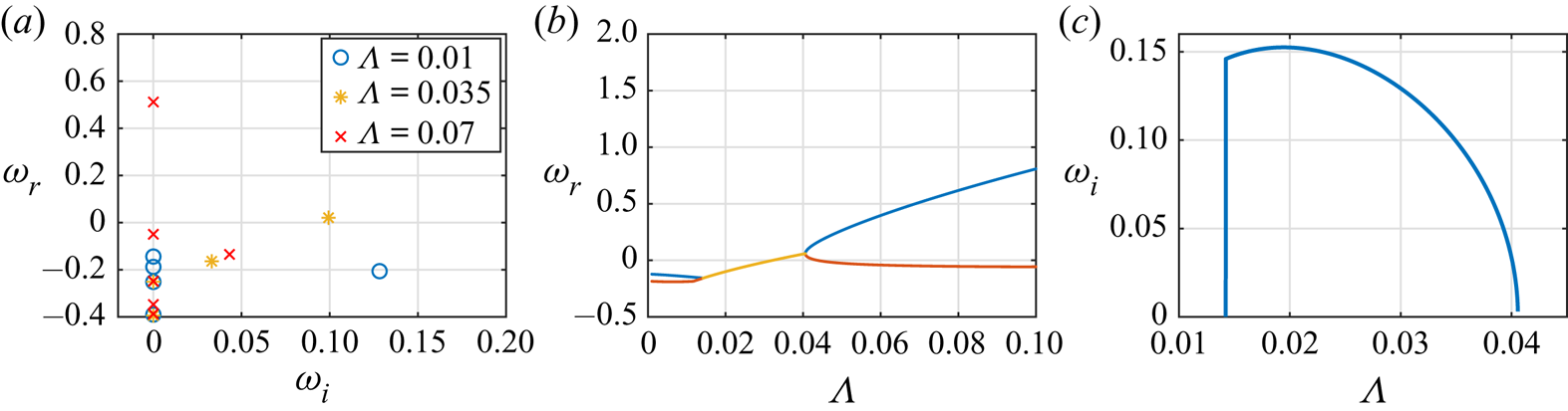
 $\varLambda$ increases gradually from zero to a value sufficiently large for instability to occur. In the current flow the concentration difference stabilizes the flow while the heat-releasing process produces unstable thermal stratification. One may speculate that for given fluid properties and concentration difference, the fluid layer becomes unstable when the heat-releasing rate is large enough. This is indeed the case, as shown in figure 1, where we plot the instability properties for a single two-dimensional mode with
 $k_x=4$ and
 $k_y=0$. In figure 1(a) we show the spectra of the most unstable modes for three different values of
 $\varLambda$. The most unstable mode refers to the mode with the largest growth rate
 $\omega _r$. For
 $\varLambda =0.01$, the most unstable mode is a stationary wave, but with decaying amplitude. However, for the mediate
 $\varLambda =0.035$, the most unstable modes become a pair of oscillatory ones with
 $\omega _i\neq 0$, and with positive growth rate. For
 $\varLambda =0.7$ the most unstable mode becomes a stationary mode again. Figure 1(b,c) show the growth rates of the most unstable modes and the oscillating frequency of the most unstable oscillatory modes versus
 $\varLambda$, respectively. For this set of parameters and wavenumber, the critical
 $\varLambda$ is around
 $0.032$, at which the oscillatory mode becomes unstable first. The oscillating frequency decreases to zero for
 $\varLambda$ slightly larger than
 $0.04$, beyond which the oscillatory mode is no longer the most unstable one.
(a) Spectrum of the most unstable modes for three different heat-releasing rates. The full spectrum is symmetric with respect to  $\omega _i=0$, so that only the right half is shown. (b) The real parts of the leading eigenvalues versus
 $\varLambda$. Blue and red lines denote the two most unstable steady modes, while the yellow line denotes oscillatory mode. (c) Variations of the imaginary parts of the eigenvalues for the oscillatory modes. For all plots
 $Pr=7$,
 $Sc=21$,
 $Ra=10^4$ and
 $k_x=4$, respectively.

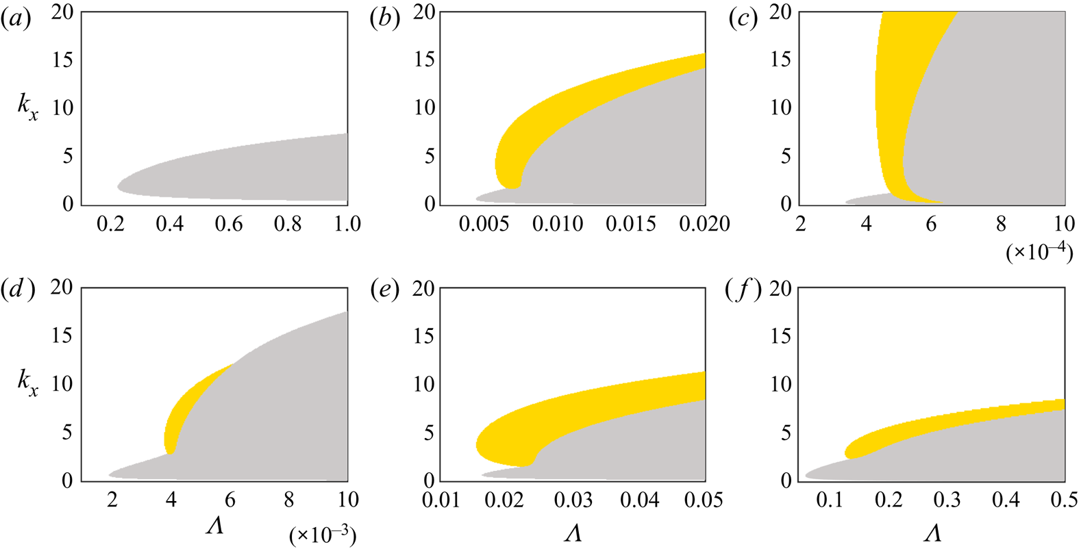
In figure 2 we plot the phase diagram on the  $\varLambda$-
 $k_x$ plane for different combinations of
 $(Sc, Ra)$. We mark the regions for unstable stationary and oscillatory modes by the grey and yellow colours, respectively. Grid independence has been checked with total nodes increased from 150 to 450 in the wall-normal direction, and the phase diagram does not change. Thus in the following we use 150 nodes. Figure 2(a–c) indicate that for fixed
 $Sc=21$, instability occurs at gradually smaller
 $\varLambda$ as
 $Ra$ increases from
 $10^3$ to
 $10^7$. When
 $Ra=10^3$, all unstable modes are stationary ones. For larger
 $Ra$, the unstable modes can be oscillatory for certain
 $\varLambda$ and wavenumbers. The unstable region expands towards large wavenumbers as
 $Ra$ becomes bigger. We then set
 $Ra=10^5$ and investigate the instability region for different Schmidt numbers, as shown in figure 2(d–f). As
 $Sc$ increases, the critical heat releasing rate
 $\varLambda _{cr}$ also increases. It is interesting to notice that at
 $Sc=100$ the most unstable mode is the oscillatory one, instead of the stationary one as for
 $Sc=10$ and
 $1000$.
The unstable region on the  $\varLambda$–
 $k_x$ plane for different combinations of
 $Ra$ and
 $Sc$. Panels (a–c) are for fixed
 $Sc=21$ and (a)
 $Ra=10^3$, (b)
 $Ra=10^5$, (c)
 $Ra=10^7$. Panels (d–f) are for fixed
 $Ra=10^5$ and (d)
 $Sc=10$, (e)
 $Sc=100$, (f)
 $Sc=1000$. The grey colour marks the unstable region with stationary modes, while the yellow colour for the region with unstable oscillatory modes, respectively.

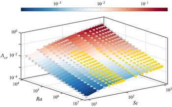
We then determine the dependence of the critical heat-releasing rate  $\varLambda _{cr}$ on
 $Ra$ and
 $Sc$, which is displayed in figure 3. Specifically, for a given pair of
 $(Ra, Sc)$ we calculate the phase diagram as shown in figure 2. The critical value
 $\varLambda _{cr}$ is the minimal
 $\varLambda$ with unstable mode. Overall
 $\varLambda _{cr}$ decreases with
 $Ra$ and increases with
 $Sc$. For
 $Ra\gtrapprox 10^5$ there exist a range of
 $Sc$ where the unstable mode associated with the critical heat-releasing rate is oscillatory, as marked by the yellow circles.
The critical heat releasing rate  $\varLambda _{cr}$ versus
 $Ra$ and
 $Sc$. The colour map represents the value of
 $\varLambda _{cr}$. The grey squares mark the cases with stationary mode, while the yellow circles with the oscillatory mode, respectively.

Before proceeding to the fully developed flows, we compare the two-dimensional linear DNS with the fully nonlinear one for  $Sc=21$,
 $Ra=10^4$,
 $\varLambda =0.027$ and
 $k_x=1$. The domain width is set as
 $2{\rm \pi}$ to accommodate one wave pattern. We numerically integrate the linearized equation (3.2) and the fully nonlinear one (2.2) separately. The initial condition for the former is small random perturbations, while that for the latter is the base flow (3.1a,b) superposed with small random perturbations. Due to the domain width, the mode with
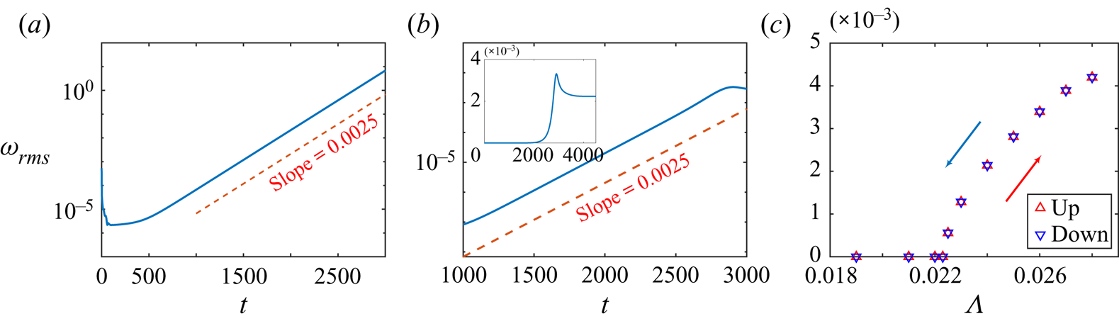
 $k_x=1$ will dominate the linearly growing stage and set the corresponding growth rate. The growth rates of the r.m.s. value of vertical velocity
 $w_{rms}$ are compared and shown in figure 4(a,b). Both the linear and nonlinear simulations give the same growth rate at the initially linear stage. Here
 $w_{rms}$ eventually saturates in the fully nonlinear simulation. To further reveal the nature of the instability, we calculate the bifurcation diagram around the critical
 $\varLambda _{cr}$. Specifically, we calculate
 $w_{rms}$ at the fully developed two-dimensional nonlinear simulation with successively increasing or decreasing
 $\varLambda$. As shown in figure 4(c),
 $w_{rms}$ follows the same path for both increasing and decreasing
 $\varLambda$, indicating a supercritical bifurcation of the system.
Temporal evolution of  $w_{rms}$ calculated by (a) two-dimensional linear DNS and (b) nonlinear DNS for
 $Pr=7$,
 $Sc=21$,
 $Ra=10^4$,
 $k_x=1$ and
 $\varLambda =0.027$, respectively. The slope is obtained by curve fitting of the linear segment, which is consistent with the results given by the linear stability analysis. Inset in panel (b) displays the whole nonlinear development. (c) The bifurcation diagram around
 $\varLambda _{cr}$ for the same parameters. Upward and downward triangles, along with the two arrows, indicate successively increasing and decreasing
 $\varLambda$.

4. Fully developed convection flows
4.1. Numerical settings and explored parameter space
We now turn to the fully developed flow. As mentioned before,  $Pr$ and
 $Sc$ are fixed at
 $7$ and
 $21$, respectively. We systematically increase
 $Ra$ from
 $10^4$ to
 $10^7$, and for each
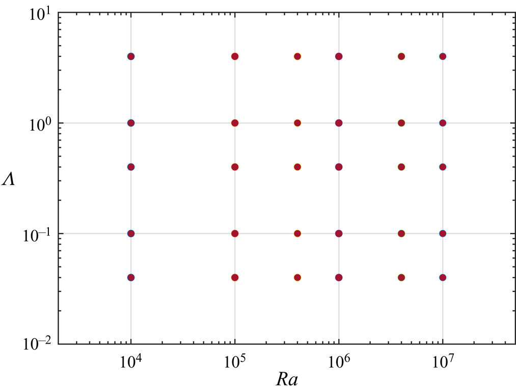
 $Ra$ we simulate five cases with
 $\varLambda$ ranging between
 $0.04$ and
 $4.0$. The explored phase space on the
 $Ra$–
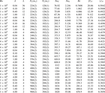
 $\varLambda$ plane is shown in figure 5. The numerical details and global responses are summarized in table 1.
The phase space explored in the current simulations. For all cases  $Pr=7$ and
 $Sc=21$, respectively.

Summary of the simulated cases. Columns from left to right are the concentration Rayleigh number, the non-dimensional heat-releasing rate, the aspect ratio of the domain, the resolutions in the horizontal and vertical directions (with refinement coefficients for multiple resolutions), the Nusselt numbers of temperature and concentration, the Reynolds number based on the r.m.s. value of velocity, the volume averaged temperature and concentration, respectively. The resolution in the y direction is the same as that in the x direction. For all cases Pr = 7 and Sc = 21.

It should be pointed out that in our simulations the domain width changes for different cases. In the RB flow, it is well know that the domain width has non-negligible effect on the global transport (Funfschilling et al. Reference Funfschilling, Brown, Nikolaenko and Ahlers2005; Bailon-Cuba, Emran & Schumacher Reference Bailon-Cuba, Emran and Schumacher2010; Krug, Lohse & Stevens Reference Krug, Lohse and Stevens2020). Here to save computing cost, we always choose the domain width larger than the width of the convection cells developed in the domain. Our results suggest that, as  $Ra$ and
 $\varLambda$ increase, the width of convection cells decreases, and the domain width is reduced accordingly. Moreover, for
 $Ra=10^5$ and
 $\varGamma =0.1$, three different domain widths are tested for
 $8H$,
 $12H$ and
 $16H$. The differences in the global responses are less than
 $3\,\%$. The exact aspect ratio used for each case is also given in table 1.
As a reference for the discussion below, we use linear stability analysis to determine the critical concentration Rayleigh number and corresponding wavenumber for  $Sc=21$ and the five heat-releasing rates simulated in DNS, see table 2. The concentration Rayleigh number in DNS is well above the critical value for simulated
 $\varLambda$.
The critical concentration Rayleigh number  $Ra_{cr}$ and the corresponding wavenumber
 $k_{cr}$ calculated by linear stability analysis for all the heat-releasing rates simulated in DNS. For all cases
 $Pr=7$ and
 $Sc=21$.

4.2. Flow structures and mean statistics
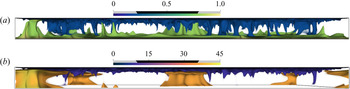
The typical convection structures in the current system are illustrated in figure 6 by the volume rendering of the two scalar components for the case with  $Ra=10^5$ and
 $\varLambda =0.1$. We only show the regions with
 $\theta$ and
 $c$ smaller than
 $20\,\%$ and larger than
 $80\,\%$ of the respective maximums. The structures which grow from the bottom boundary form isolated columns with large horizontal length scales and extend to the top boundary. Those originated from the top boundary are scattered small plumes.
Three-dimensional volume rendering of (a) concentration and (b) temperature fields for the case with  $Ra=10^5$ and
 $\varLambda =0.1$. For both components, we show the values smaller than
 $20\,\%$ and larger than
 $80\,\%$ of the maximal value.

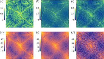
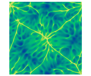
The asymmetry between the columns from the bottom and the plumes from the top can also be observed in the horizontal slices at different heights, see figure 7. Near the bottom plate, the high concentration and temperature regions form several very long and thin filaments. At the intersections of filaments, columns rise vertically and carry high concentration and temperature into the bulk. Near the top boundary, however, low concentration and temperature filaments are much shorter and form complex networks. Scattered plumes then descend from these filaments.
Concentration (a–c) and temperature (d–f) on three horizontal slices at different heights for the case with  $Sc=21$,
 $Pr=7$,
 $Ra=10^5$ and
 $\varLambda =0.1$. For panels (a,d), (b,e) and (c,f) we have
 $z/H=0.1$,
 $0.5$ and
 $0.9$, respectively.

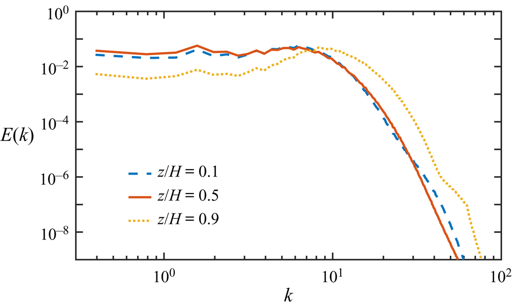
To demonstrate the different length scales near the top and bottom plates, we show in figure 8 the time-averaged one-dimensional energy spectra of the vertical velocity  $w$ at three horizontal planes at different heights, namely
 $z/H=0.1$,
 $0.5$ and
 $0.9$, for the case shown in figures 6 and 7. The energy spectra are normalized by their total energy. The spectra at the two lower planes are very similar to each other, but they are very different compared with that of the plane at
 $z/H=0.9$, which is close to the top plate. Clearly, among the three planes, the energy spectrum of the top one has lowest energy at small wavenumbers, and highest energy at large wavenumbers. Therefore, the most energetic scales near the top plate are smaller than those near the bottom plate. This is consistent with the volume rendering shown in figure 6.
Energy spectra of vertical velocity  $w$ on three horizontal slices at different heights for the case with
 $Sc=21$,
 $Pr=7$,
 $Ra=10^5$, and
 $\varLambda =0.1$. The spectra have been averaged over the horizontal slice and time.

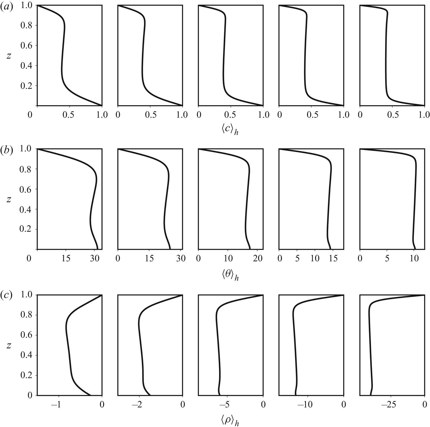
In figure 9 the mean profiles of temperature  $\langle \theta \rangle _h$ and concentration
 $\langle c\rangle _h$ are shown for
 $Ra=10^5$ and
 $\varLambda$ from
 $0.04$ to
 $4$, with
 $\langle \cdot \rangle _h$ standing for the average over horizontal slices and time. Three regions can be identified at different heights. Just below the top plate, strong vertical gradients develop in both concentration and temperature profiles. Near the bottom plate, the mean concentration profile has strong gradient, while the temperature gradient is visible but relatively weak. In-between, a bulk region exists with nearly constant concentration and temperature. For increasing
 $\varLambda$ the mean concentration in the bulk exhibits minor changes, but the mean temperature decreases considerably. The decrease of bulk temperature is mainly due to the non-dimensionalization, namely, higher
 $\varLambda$ corresponding to a larger characteristic temperature scale
 $\varDelta _T$. The mean profiles for density
 $\langle \rho \rangle _h$ are shown in figure 9(c). In the bulk the total density is weakly stably stratified. In the top boundary region, the mean gradient of density is unstable. While in the bottom boundary region, it is stable for small
 $\varLambda$ but unstable when
 $\varLambda$ is large enough.
Mean profile of (a) concentration, (b) temperature and (c) density for  $Ra=10^5$ and different
 $\varLambda$. Subpanels from left to right correspond to
 $\varLambda =0.04$,
 $0.1$,
 $0.4$,
 $1$ and
 $4$, respectively.

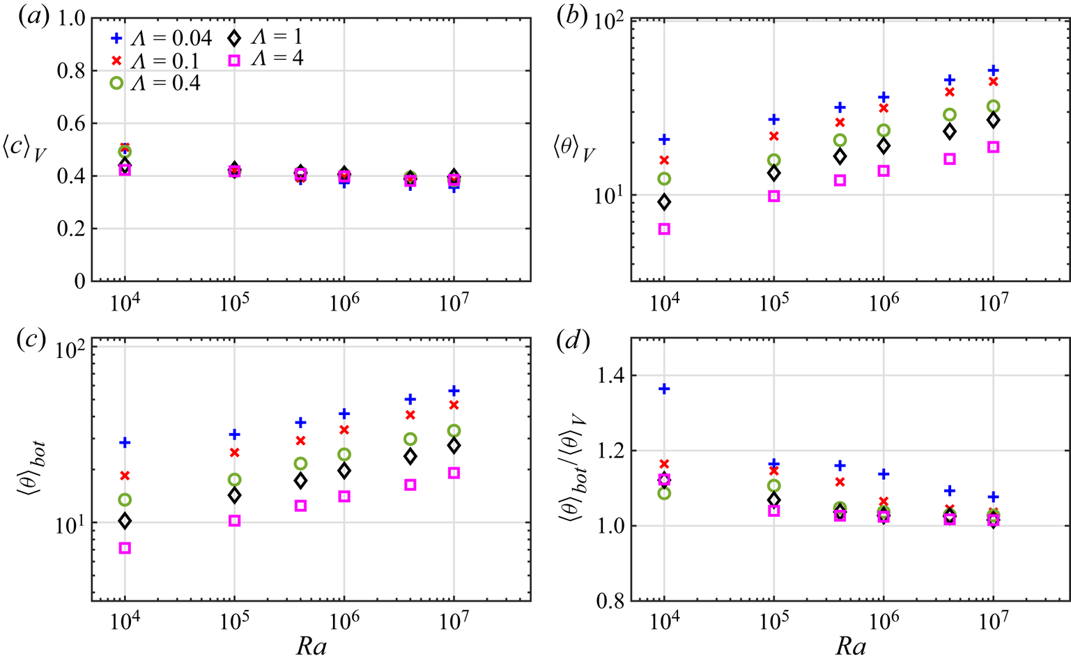
The dependences of the volume-averaged concentration  $\langle c \rangle _V$ on
 $Ra$ and
 $\varLambda$ are plotted in figure 10(a). Interestingly,
 $\langle c \rangle _V$ only shows minor variations and is close to the value
 $0.4$. This is mainly due to the fact that in the bulk region
 $c$ is almost constant and close to
 $0.4$, as indicated by figure 9(a). The concentration in the two boundary layers deviates from the bulk value. However, the top and bottom boundary layers make opposite contributions to the volume average of
 $c$, and they become thinner as
 $Ra$ and
 $\varLambda$ increase. Therefore, we see that in figure 10(a),
 $\langle c \rangle _V$ is more scattering for different
 $\varLambda$ at low
 $Ra$. The volume averaged temperature
 $\langle \theta \rangle _V$ is plotted in figure 10(b), along with the averaged temperature at the bottom plate
 $\langle \theta \rangle _{bot}$ shown in figure 10(c). Both
 $\langle \theta \rangle _V$ and
 $\langle \theta \rangle _{bot}$ increase as
 $Ra$ becomes larger. For fixed
 $Ra$ they decrease with increasing
 $\varLambda$, which is again due to the fact that the characteristic temperature
 $\varDelta _T$ increases with
 $\varLambda$. Since
 $\langle \theta \rangle _V$ and
 $\langle \theta \rangle _{bot}$ share similar dependences on
 $Ra$ and
 $\varLambda$, the ratio between them, i.e.
 $\langle \theta \rangle _{bot}/\langle \theta \rangle _V$, approaches unit when
 $Ra$ and
 $\varLambda$ increase, as shown in figure 10(d).
(a) Volume averaged concentration  $\langle c \rangle _V$, (b) volume averaged temperature
 $\langle \theta \rangle _V$, (c) average temperature at the bottom plate
 $\langle \theta \rangle _{bot}$ and (d) the ratio
 $\langle \theta \rangle _{bot}/\langle \theta \rangle _V$ versus
 $Ra$ and
 $\varLambda$, respectively.

4.3. Total fluxes of the system
We now look at the global transport properties, namely the two Nusselt numbers and the Reynolds numbers defined in (2.6a–c). The dependences of these quantities on  $Ra$ and
 $\varLambda$ are shown in figure 11. Both
 $Nu_C$ and
 $Re$ increase as either
 $Ra$ or
 $\varLambda$ increases. This is expected since larger total concentration difference or heat-releasing rate induces stronger flow motion and concentration flux. The temperature Nusselt number exhibits very interesting behaviour. It increases with
 $Ra$, but shows minor dependence on
 $\varLambda$ for fixed
 $Ra$. For fixed
 $Ra$, higher
 $\varLambda$ should generate more heat and, therefore, stronger heat flux through the top plate. Notice that in (2.6a–c) the definition of
 $Nu_T$ is the total heat flux non-dimensionalized by
 $\kappa _T\varDelta _TH^{-1}$. Then the increasing of the dimensional heat flux is compensated by the increasing of
 $\varDelta _T$, which results in a very weak dependence of
 $Nu_T$ on
 $\varLambda$.
The global responses versus the control parameters. The upper and bottom rows show the dependence of the same data set on  $Ra$ and
 $\varLambda$, respectively. The dashed lines and corresponding slopes mark the scaling laws predicted by the unifying model.

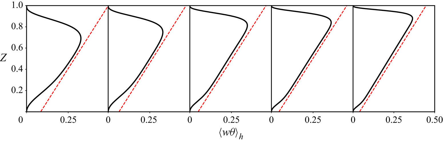
In figure 12 we plot the mean profiles of convective heat flux  $\langle w \theta \rangle _h$. All the profiles have a distinct linear segment in the bulk region, showing that the convective flux increases linearly with height. This can be understood by taking the horizontal and temporal average of the temperature (2.2c). For the statistically steady state, one has
 \begin{equation} \frac{\textrm{d} \langle w\theta \rangle_h}{\textrm{d} z} = \frac{\sqrt{Sc}}{Pr\sqrt{Ra}} \frac{\textrm{d}^2 \langle \theta \rangle_h}{\textrm{d} z^2} + \langle c \rangle_h. \end{equation}
Figure 9 indicates that in the bulk region the mean temperature is approximately a linear function of height and the concentration is nearly constant. Then, in the above equation the first term on the right-hand side vanishes, and one obtains
 \begin{equation} \langle w\theta \rangle_h \sim \langle c \rangle_{bulk} z,\end{equation}
with  $\langle c \rangle _{bulk}$ being the mean concentration in the bulk region. Thus, the convective flux
 $\langle w\theta \rangle _h$ depends linearly on
 $z$ in the bulk region with a slope of
 $\langle c \rangle _{bulk}$, which is exactly the case as shown in figure 12.
Mean profiles of  $\langle w \theta \rangle _h$ for when
 $Ra=10^5$. For panels from left to right we have
 $\varLambda =0.04$,
 $0.1$,
 $0.4$,
 $1$ and
 $4$, respectively. The dotted line is the reference line whose slope is
 $1/\langle c \rangle _{bulk}$.

4.4. The unifying model for transport fluxes
The dependences of the global responses, namely Nusselt and Reynolds numbers, on the control parameters can be explained by extending the unifying theory for the RB flows (Grossmann & Lohse Reference Grossmann and Lohse2000, Reference Grossmann and Lohse2001, Reference Grossmann and Lohse2002, Reference Grossmann and Lohse2004) to the current system. The procedure is very similar to that reported in Wang et al. (Reference Wang, Lohse and Shishkina2020). Here we only briefly describe the theoretical derivation, and then compare our results with the theoretical model.
We start from the exact global balance relations for the dissipation rates of momentum and two scalars (Shraiman & Siggia Reference Shraiman and Siggia1990), which can be readily obtained for the current flow as
 $$\begin{gather} \epsilon_u = \nu\langle(\partial_i u_j)^2\rangle_V = \frac{\nu^3}{H^4} Ra^{{3}/{2}}Sc^{-{3}/{2}}(\varLambda\langle w\theta \rangle_V-\langle w c \rangle_V), \end{gather}$$
 $$\begin{gather}\epsilon_c = \kappa_c\langle(\partial_i c)^2\rangle_V = \kappa_c(\varDelta_C)^2H^{{-}2}Nu_C, \end{gather}$$
 $$\begin{gather}\epsilon_{\theta} = \kappa_\theta\langle(\partial_i \theta)^2\rangle_V = \lambda\frac{\varLambda (\varDelta_C)^2 H}{\sqrt{g\beta_C\varDelta_C H}} \langle\theta c\rangle_V. \end{gather}$$
The last term in (4.5) comes from the heat releasing term and involves the cross-correlation between temperature and concentration, on which is difficult to conduct a scaling analysis. In the following discussion, we mainly make use of the first two relations (4.3) and (4.4). Following the idea of the GL theory (Grossmann & Lohse Reference Grossmann and Lohse2000, Reference Grossmann and Lohse2001, Reference Grossmann and Lohse2002, Reference Grossmann and Lohse2004), each dissipation rate can be decomposed into the contributions from the boundary layer and bulk regions as
 \begin{equation} \epsilon_u= \epsilon_u^{BL} +\epsilon_u^{bulk}, \quad \epsilon_c= \epsilon_c^{BL} +\epsilon_c^{bulk}. \end{equation}
The scaling laws for each part of the dissipation rate can then be estimated by scaling analysis. Due to the large  $Sc$ and relatively low
 $Ra$, we assume that both
 $\epsilon _u$ and
 $\epsilon _c$ are dominated by the boundary layer contribution.
Denote the boundary layer thickness by  $\lambda _u$ for the momentum field and
 $\lambda _c$ for the concentration field, respectively. The thickness of a laminar boundary layer has the scaling
 $\lambda _u \sim H/\sqrt {Re}$, and the dissipation rate can be estimated as
 \begin{equation} \epsilon_u^{BL} \sim \nu \left(\frac{U}{\lambda_u}\right)^2 \frac{\lambda_u}{H} = \frac{\nu^3}{H^4} Re^{5/2}. \end{equation}
Then by the global balance of (4.3) and neglecting  $\epsilon _u^{bulk}$, one has
 \begin{equation} Re^{5/2}\sim Ra^{3/2}Sc^{{-}3/2}(\varLambda\langle w\theta \rangle_V - \langle w c \rangle_V). \end{equation}
The concentration dissipation rate from the two boundary layer regions can be similarly estimated as (Wang et al. Reference Wang, Lohse and Shishkina2020)
 \begin{equation} \epsilon_c^{BL} \sim \kappa_c\left(\frac{\varDelta_C}{\lambda_c}\right)^2\frac{\lambda_c}{H} = \kappa_c\frac{\varDelta_C^2}{H^2} \frac{\lambda_u}{\lambda_c}Re^{1/2}, \end{equation}
and for large  $Sc$ regime, one has
 $\lambda _u/\lambda _c \sim Sc^{1/3}$ for a laminar boundary layer. Substitute this scaling into the above equation, and using the global balance for concentration dissipation rate, one obtains the following scaling:
 \begin{equation} Nu_C \sim Sc^{1/3}Re^{1/2}. \end{equation}
The scaling relation (4.8) can be further simplified. First, figure 10 suggests that in the flow domain  $c$ is much smaller than
 $\theta$. Since both
 $\theta$ and
 $c$ are transported by the same velocity field, they correlate to the vertical velocity
 $w$ in a similar way, and
 $\langle w c \rangle _V$ should also be much smaller than
 $\varLambda \langle w \theta \rangle _V$ as long as
 $\varLambda$ is not very small. Then the second term inside the parenthesis on the right-hand side of (4.8) is negligible. Next, by (4.2) and approximating
 $\langle c \rangle _{bulk}$ by
 $\langle c \rangle _V$, one has
 \begin{equation} \langle w \theta \rangle_V \approx \frac{1}{H} \langle c \rangle_V \int_0^H z \, \textrm{d} z = \frac{1}{2} \langle c \rangle_V, \end{equation}
and the scaling relation becomes
 \begin{equation} Re = A_1 Sc^{{-}3/5} Ra^{3/5} \varLambda^{2/5}, \end{equation}
where we have absorbed  $\langle c \rangle _V$ into the prefactor constant
 $A_1$ since for all the cases the volume averaged concentration is very close to each other. Then by (4.10) the scaling law for
 $Nu_C$ reads
 \begin{equation} Nu_C = A_2 Sc^{1/30} Ra^{3/10} \varLambda^{1/5}. \end{equation}
For the thermal Nusselt number one can directly obtain the following scaling by performing the volume integral of (2.2c) for the statistically steady state:
 \begin{equation} Nu_T=\langle\partial_z\theta\rangle_{top}=A_3 Sc^{{-}1/2} Pr Ra^{1/2}, \end{equation}
in which we have used again the fact that the volume averaged concentration is nearly constant.
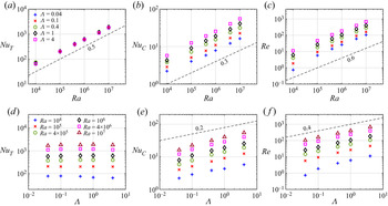
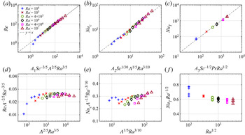
Equations (4.12)–(4.14) are the main results of our theoretical model. In figure 13(a–c) the three scaling laws are compared with our numerical results. The prefactors  $A_1\approx 0.15$ and
 $A_2\approx 0.27$ are determined by data fitting, while
 $A_3$ is manually set at
 $0.4$, i.e. close to the value of
 $\langle c \rangle _V$. All the data points collapse and agree well with the proposed scaling laws. We further examine the scaling laws by plotting the data in the compensated way, see figure 13(d–f), which reveals that the theoretical model exhibit some minor errors, especially at small
 $Ra$ for
 $Re$ and
 $Nu_T$. The error at small
 $Ra$ is mainly introduced by replacing
 $\langle c \rangle _{bulk}$ with
 $\langle c \rangle _V$. As indicated by figure 10(a), the difference between the two averaged values is highest at small
 $Ra$.
(a–c) The comparison between the numerical data and the scaling laws given by the theoretical model. The values of the prefactors are  $A_1=0.15$,
 $A_2=0.27$ and
 $A_3=0.4$, respectively. (d–f) The compensated plots of the same dataset and scaling laws.

5. Conclusions
Here we conducted a systematic study about the convection flow driven by a heat releasing concentration field. The concentration field is stably stratified, so at the bottom of the fluid layer concentration is higher. Due to the heat released by the concentration component, buoyancy-driven convection may develop in the flow domain. The fluid density is assumed to be dependent on both concentration and temperature, and the heat-releasing rate is linearly proportional to the concentration.
The stability of the system is first investigated by normal-mode linear stability analysis. The critical heat releasing rate  $\varLambda _{cr}$ is identified for various fluid properties, namely Schmidt number
 $Sc$, and the concentration differences measured by the concentration Rayleigh number
 $Ra$. For fixed Prandtl number
 $Pr=7$,
 $\varLambda _{cr}$ decreases with
 $Ra$ but increases with
 $Sc$. The most unstable mode associated with the critical heat releasing rate can be either stationary or oscillatory for different control parameters. The fully nonlinear simulations around
 $\varLambda _{cr}$ reveal that the system undergoes a supercritical bifurcation.
For the fully developed flows, DNS are carried out for a series of  $Ra$ and
 $\varLambda$. The flow structures are different between those from the bottom plate and those from the top one. Large columns grow from the bottom plate and transport high temperature and concentration upward. From the top plate small plumes descend. The mean scalar profiles indicate a nearly homogeneous bulk region bounded by two boundary layer regions with strong vertical gradients. The volume averaged concentration exhibits minor dependence on both
 $Ra$ and
 $\varLambda$.
The total heat and concentration fluxes through the top plate, and the flow velocity, are affected by both concentration difference and heat-releasing rate. Based on the unifying theory for RB flow, we develop scaling laws to describe the variations of the thermal and concentration Nusselt numbers, and the Reynolds number. The numerical results agree very well with the proposed scaling laws. However, it should be noted that here we only derive the scaling laws in the I $_u$ region (e.g.
 $\epsilon ^{BL}_u$ and
 $\epsilon ^{BL}_c$ dominate and
 $Sc>1$). The applicability of the unifying model for other regions for the current system requires more systematic simulations over wider parameter range, especially for different fluid properties and higher concentration Rayleigh numbers.
Funding
This work is supported by the Major Research Plan of National Natural Science Foundation of China for Turbulent Structures under the grants 91852107 and 91752202. Y.Y. also acknowledges the partial support from the Strategic Priority Research Program of Chinese Academy of Sciences under the grant no. XDB42000000. M.Z. acknowledges the financial support from the Ministry of Education, Singapore (MOE WBS no. R-265-000-654-114).
Declaration of interest
The authors report no conflict of interest.