


Introduction
The marine-based West Antarctic ice sheet (WAIS) is drained by fast-flowing ice streams with low surface gradients and low basal shear stresses. Their fast flow is facilitated by the deformation of water-saturated subglacial sediments (Reference Alley, Blankenship, Bentley and RooneyAlley and others, 1986; Reference Tulaczyk, Kamb and EngelhardtTulaczyk and others, 2000a), despite net freeze-on of subglacial water occurring beneath large areas of the ice-stream trunks (Reference Joughin, Tulaczyk, MacAyeal and EngelhardtJoughin and others, 2004). Models that address basal processes exist at a local scale (e.g. Reference Tulaczyk, Kamb and EngelhardtTulaczyk and others, 2000b; Reference Bougamont, Tulaczyk and JoughinBougamont and others, 2003; Reference Parizek and AlleyParizek and Alley, 2004); however, a valid continental-scale model for the WAIS has not yet been developed (Reference Le BrocqLe Brocq, 2007). It is possible to reproduce the low surface slopes of the ice streams by incorporating a measure of effective pressure (e.g. ice thickness above buoyancy) into the sliding relation, along with the basal shear stress (e.g. Reference Budd, Jenssen and SmithBudd and others, 1984). However, in order to restrict the streaming flow to the ice streams, a thermal criterion has often been introduced, such that sliding occurs only where the base of the ice is at the pressure-melting point (e.g. Reference PaynePayne, 1999; Reference Le BrocqLe Brocq, 2007). This is contrary to modelled basal melt rates derived from data assimilation (Reference Joughin, Tulaczyk, MacAyeal and EngelhardtJoughin and others, 2004), suggesting that the majority of the interior of the WAIS is at the pressure-melting point. Further, Reference Joughin, Tulaczyk, MacAyeal and EngelhardtJoughin and others (2004) suggest that freeze-on can occur beneath ice streams; in order for ice streams to remain at the pressure-melting point in regions of basal freeze-on, there must be a supply of subglacial water to prevent the ice falling below the melting point. The role of subglacial water is not represented in the model formulation described above. The existence of fast ice-stream flow in areas of net freeze-on suggests either a cyclical (melt/freeze–slip/stick) behaviour of ice streams (Reference Tulaczyk, Kamb and EngelhardtTulaczyk and others 2000a), or that the redistribution of water plays a role in maintaining fast ice-stream flow despite the net basal freeze-on (Reference Parizek, Alley and HulbeParizek and others, 2003). The regulatory role of the thermal and subglacial hydrological regime is crucial to the evolution of the ice sheet, and must be represented in a physically meaningful manner in an ice-sheet flow model. The role of subglacial water in controlling ice dynamics is further underlined by the current discussion of the role of subglacial lakes in supplying periodic large volumes of water directly to fast-flow drainage features (e.g. Reference Wingham, Siegert, Shepherd and MuirWingham and others, 2006; Reference Fricker, Scambos, Bindschadler and PadmanFricker and others, 2007; Reference Stearns, Smith and HamiltonStearns and others, 2008), and the existence of subglacial lakes at fast-flow onset zones (e.g. Reference Siegert and BamberSiegert and Bamber, 2000; Reference Bell, Studinger, Shuman, Fahnestock and JoughinBell and others 2007).
The role of subglacial water in regulating ice flow has a long research history in both alpine and ice-sheet environments (see next section). However, converting this research into an appropriate model of subglacial water flow for coupling with an ice-flow model for an ice sheet is still at an early stage of development. The large majority of previous attempts propose the use of, or are based on, a Weertmantype water ‘film’ as a parameterization of the subglacial water system (Reference WeertmanWeertman, 1966, Reference Weertman1972; Reference Weertman and BirchfieldWeertman and Birchfield, 1982; Reference Budd, Jenssen, Van der Veen and OerlemansBudd and Jenssen, 1987; Reference AlleyAlley, 1989, Reference Alley1996; Reference Johnson and FastookJohnson and Fastook, 2002). Reference Arnold and SharpArnold and Sharp (2002) introduce a representation of subglacial channels into their model, although, at a model resolution of 40 km, this is more a parameterization of the nature of the subglacial hydrological system than a physically based representation of the channels themselves. In the above models, the sliding velocity of the ice is proposed to be a function of the subglacial water depth (except for Reference Arnold and SharpArnold and Sharp (2002), where the sliding is a function of water pressure). The strength of this type of parameterization is that it is conceptually simple, relatively inexpensive computationally, and applicable in coarse-resolution modelling. It is clear from the review, presented below, and the subsequent model description, however, that the model applied in this paper is a simple parameterization of a complex system, and contains a number of assumptions relating to the nature of the subglacial water flow.
None of the above models have been validated against measured data, so it is only possible to investigate the impact that the subglacial water has on the model output. Since this previous research, a large amount of data, against which to evaluate such a model, has become available for the WAIS. These datasets include ice velocity (Reference Joughin, Tulaczyk, Bindschadler and PriceJoughin and others, 2002), basal melt rates (from data inversion) (Reference Joughin, Tulaczyk, MacAyeal and EngelhardtJoughin and others, 2004) and accurate surface topography (Reference Bamber, Gomez-Dans and GriggsBamber and others, 2009). The aim of this paper is to revisit the thinfilm-based model of subglacial hydrology and to evaluate the potential of the model for improving ice-flow model simulations of the WAIS in particular, using the newly available data.
A brief review of previous research into subglacial water systems is provided in the next section, and a description of the model applied in this work given. The subglacial water-flow model is then applied to the present-day configuration of the Ross Sea sector of the WAIS (Fig. 1) to derive the equilibrium water depth. The model utilizes two schemes – a time-dependent scheme and a steady-state scheme – and two resolutions – 20 km and 5 km. The potential for coupling the subglacial water-flow model with an ice-sheet model is then outlined and discussed.
Location map showing the Ross Sea ice streams. Interferometric synthetic aperture radar (InSAR) velocity (from Reference Joughin, Tulaczyk, Bindschadler and PriceJoughin and others, 2002) overlaid on a hillshade of the surface digital elevation model (Reference Bamber, Gomez-Dans and GriggsBamber and others, 2009). Velocity contours shown are 25 m a−1(thin line) and 250 m a−1(thick line); coastline is from Antarctic Digital Database version 3, and the dashed line marks the margin of the formerly fast-flowing Kamb Ice Stream.

Background
There are many possible mechanisms for water transport beneath an ice sheet. Four different methods of water flow beneath glaciers were proposed around the early 1970s: (1) R channels, incised into the ice (Reference RöthlisbergerRöthlisberger, 1972); (2) N channels, incised into the bedrock (Reference NyeNye, 1973); (3) in a water film, mm in depth (Reference WeertmanWeertman, 1966, Reference Weertman1972); and (4) in a linked cavity system (Reference LliboutryLliboutry, 1968). These first theories of subglacial water flow were concerned with the flow between the ice and the bedrock; flow in the underlying substrate was not initially considered. Reference Walder and FowlerWalder and Fowler (1994) proposed that a distributed system of broad canals may form in the sediment. There is also the possibility of aquifer flow in the sediment, though it is usually not considered to have the capacity required to transport significant amounts of meltwater (Reference Lingle, Brown, Van der Veen and OerlemansLingle and Brown, 1987). The important distinction between these mechanisms concerns those that are channelized and those that are distributed. In a distributed system, the effective pressure is low (the water pressure approaches the ice overburden pressure) and the effective pressure decreases with increasing discharge. In a channelized system, the effective pressure is high, and increases with increasing discharge.
A link between the subglacial water and the sliding velocity of an ice sheet was acknowledged by Reference WeertmanWeertman (1964), observing that a water layer with a thickness an order of magnitude smaller than the controlling obstacle size can cause an appreciable increase in the sliding velocity. Weertman’s initial theory was extended by Lliboutry (e.g. Reference LliboutryLliboutry, 1968), who pointed out that water-filled cavity formation on the downstream side of protuberances would affect the sliding velocity through the decoupling of the ice and the bed. Reference WeertmanWeertman (1964) proposed a modified relation for the sliding velocity, incorporating the effect of the water layer into the roughness estimation. Reference Weertman and BirchfieldWeertman and Birchfield (1982) applied the model in a theoretical framework, to infer the impact of a water layer on WAIS stability. Reference Budd, Jenssen, Van der Veen and OerlemansBudd and Jenssen (1987) extended this work by calculating the equilibrium water depth for the Ross Sea sector of the WAIS. Using a temperature model and balance-velocity estimations (assuming steady-state conditions), they calculated basal temperatures and melt rates for the Ross Sea sector. The resulting water depths reach 10 mm under the ice streams, but are much less under the rest of the ice sheet. Reference Budd, Jenssen, Van der Veen and OerlemansBudd and Jenssen (1987) correlated the water depth, balance velocity and basal shear stress for the Ross Sea sector, and suggest that the basal traction parameter in the ice-flow model could be made a simple function of the water-film thickness.
Since the work of Reference Budd, Jenssen, Van der Veen and OerlemansBudd and Jenssen (1987), understanding of the role of subglacial water in the WAIS has developed, with deformation of water-saturated subglacial sediments identified in facilitating fast flow in the Ross Sea sector (Reference Alley, Blankenship, Bentley and RooneyAlley and others, 1986; Reference Tulaczyk, Kamb and EngelhardtTulaczyk and others, 2000a). Reference Tulaczyk, Kamb and EngelhardtTulaczyk and others (2000a) demonstrated that the yield strength of the sediment was a function of the water content of the sediment; the higher the water content of the sediment was, the lower the yield strength and, hence, the faster the ice sliding velocity (here the term ‘sliding velocity’ incorporates all types of basal ice motion, including sliding over the substrate and via deformation of the substrate). This means that for parts of the WAIS, it is the water in the underlying substrate that is important in regulating sliding velocity, rather than the water between the underlying substrate and the ice. The controlling factor in the sliding velocity is still the water availability (rather than the water pressure), so the water depth from the water-film model could be a useful proxy for the subglacial water content of the sediments beneath parts of the WAIS. The work presented here revisits that of Reference Budd, Jenssen, Van der Veen and OerlemansBudd and Jenssen (1987), with the benefit of more and better-quality data and an improved perspective on the requirements of a subglacial water-flow model for coupling with an ice-flow model.
Model Description
The model applied here is the most simplistic form of the ‘Weertman’ water-film model (following Reference Budd, Jenssen, Van der Veen and OerlemansBudd and Jenssen (1987) and the suggestions of Reference AlleyAlley (1996)). The subglacial water-flow model assumes that water flows in a thin film of water, of the order of mm thickness. The evolution of the water-film depth (d) is given by

where t is time, M is the basal melt rate (negative values indicate basal freeze-on) and u w is the depth-averaged water velocity vector (bold indicates two-dimensional horizontal vector), calculated using a theoretical treatment of laminar flow between two parallel plates, driven by differences in the water pressure (see, e.g., the appendix of Reference WeertmanWeertman, 1966):
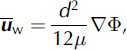
where μ is the viscosity of water and Φ is the hydraulic potential. The hydraulic potential is a function of the elevation potential and the water pressure, and is calculated using

where ρ w is the density of water, g is the acceleration due to gravity, h is the bedrock elevation and p w is the water pressure. The water pressure, p w, is a function of the ice overburden pressure and the effective pressure:

where ρ i is the density of ice, H is the ice thickness and N is effective pressure. In a channelized system, the water pressure will be less than the ice overburden pressure, so N will be non-zero. In a distributed system, however, the water pressure will be close to, if not at, the overburden pressure. As a result, a simplification can be made to Equation (4), assuming N to be zero (see, e.g., Reference Budd, Jenssen, Van der Veen and OerlemansBudd and Jenssen, 1987; Reference AlleyAlley, 1996).
The assumption that N is zero simplifies the calculation of the hydraulic potential surface by removing the need to calculate the water pressure. With this simplification, combining and rearranging Equations (3) and (4) (rewriting in terms of the upper and lower ice-surface elevations) gives the gradient of the potential surface as

where s is the ice surface elevation. Equation (4) demonstrates the well-known result that the potential gradient is mainly governed by the ice surface gradient; it is ∼10 times more important than the bedrock gradient (as ρ i = 0.91 × 10³ kg m−3 and (ρ w − ρ i) = 0.09 × 10³ kg m−3). Ice streams generally occupy bedrock troughs, and have a relatively low surface elevation (due to drawdown from fast flow), so their hydraulic potential will be lower than beneath the adjacent areas. As a result, meltwater generated at the base of the ice in the WAIS will be directed to the beds of the ice streams (Reference Weertman and BirchfieldWeertman and Birchfield, 1982).
Time-dependent vs steady-state approach
Equation (1) can be solved in two ways, either using a time-dependent approach, where ∂d/∂t is calculated and solved using a numerical technique, or a steady-state approach, which assumes that ∂d/∂t = 0. In a coupled ice/water flow model, the steady-state approach leads to the assumption that the water system reaches equilibrium within the timescale of ice response; hence, only a steady-state ‘snapshot’ of the subglacial water system is required. This has the benefit of reducing computational expense, though it will reduce the level of interaction of the ice and subglacial water systems. The following discussion presents evidence suggesting that the steady-state approach is a reasonable assumption given the difference in the timescales over which ice and water flow.
WAIS ice velocities range from <1 to around 1500 m a−1 (e.g. Reference Whillans, Bolzan and ShabtaieWhillans and others, 1987; Reference Joughin, Tulaczyk, Bindschadler and PriceJoughin and others, 2002). A direct measurement of subglacial water velocity was made using a salt tracing experiment at a location on Whillans Ice Stream (Reference Engelhardt and KambEngelhardt and Kamb, 1997). A salt solution was released from the base of a borehole, and the electrical resistance between electrodes in two downstream boreholes was measured. A sharp decrease in the electrical resistance between the boreholes was observed 2.4 hours after release, giving an average propagation velocity of 7.5 × 10⁻³ m s−1 (∼200 × 103 m a−1; Reference Engelhardt and KambEngelhardt and Kamb, 1997). Reference Wingham, Siegert, Shepherd and MuirWingham and others (2006) calculate the velocity of water in a subglacial tunnel during a lake drainage event (inferred from isolated surface elevation changes) to be 0.1–2.1 m s−1. Although this is an extreme example due to the high volume of water transferred (and flow in a tunnel will not be governed by the laminar flow assumption in the water film), it illustrates the potential difference in the flow timescales of ice and water. Taking the longest travel path in the WAIS for interior subglacial melt as ∼700 km, and assuming a water velocity of ∼1 × 10⁻² m s−1, the interior melt would take ∼2 years to reach the grounding line. This implies that the timescale of response to a perturbation in the subglacial water system is relatively short. The response time of an ice mass to a perturbation will be much longer, of the order of decades (e.g. Reference Payne, Vieli, Shepherd, Wingham and RignotPayne and others, 2004).
Both a steady-state and time-dependent approach to solving for the subglacial water depth will be demonstrated here. As only the present-day equilibrium subglacial water distribution is calculated here, the results will indicate whether the numerical scheme has an impact on the resulting subglacial water distribution.
Time-dependent approach
In order to solve Equation (1) for the evolution of the water depth (d) over time (time-dependent approach), a numerical scheme is required. Initially a Lax–Wendroff scheme was tested; however, in one-dimensional testing, this proved to be numerically unstable except at very small time-steps due to the often steep gradients in the potential surface and, hence, the water depth. Instead, a first-order upwind scheme was tried and proved to be stable at much larger time-steps, due to the implicit diffusion introduced by the scheme (Reference PressPress, 2007). The hydraulic potential surface may have sinks or hollows occurring in it; if these sinks are left unaltered, infinite water depths will build up in these locations. The sinks may indicate the presence of subglacial lakes, areas of basal freezing, or may be due to the resampling of the data to a coarse resolution, or simply errors in the topography datasets. In order to make a complete hydrological connection to the grounding line, these sinks are artificially filled using a filling algorithm. The filling algorithm assigns the average of the four immediate neighbours to the sink gridcell, repeating the process until a complete hydrological connection between upstream and downstream coastal areas can be achieved (see, e.g., Reference Budd and WarnerBudd and Warner, 1996).
Steady-state approach
Taking ∂d/∂t = 0 in Equation (1) (steady-state approach), it is possible to use a flux balance approach to calculate the steady-state water depth (in a similar way to balance-velocity calculations; see, e.g., Reference Budd and WarnerBudd and Warner (1996) or Reference Le Brocq, Payne and SiegertLe Brocq and others (2006), for more details).
Considering a grid-based balance approach, the balance flux equation for each cell is

where ψ out is the total flux out of the cell (m3 a−1), ψ in is the flux into the cell, and r is the cell edge length (assuming a square cell). In other words, the balance approach requires that the outgoing water flux from an area is equal to the incoming flux plus the melt rate in the area.
Taking the outgoing flux as an approximation for the flux through a cell, the balance equation can be stated in terms of the water depth and velocity

where l is the unit width, dependent on the flow direction through the gridcell. The flow direction relative to the grid orientation (θ) is calculated by fitting a plane to the elevations of the four neighbouring cells, and l is then calculated using

The incoming flux to each gridcell, ψ in, can be calculated using an upstream flow-routing algorithm (Reference Budd and WarnerBudd and Warner, 1996; Reference Le Brocq, Payne and SiegertLe Brocq and others, 2006), and corrected for the unit width, l; hence, Equation (7) can be written as

The flux through the cell now has units of m2 a−1 per unit width. Combining Equations (2) and (9) and rearranging for d gives

where Q l represents the upstream flux from the left-hand term in Equation (9).
The calculation of the upstream flux is independent of the water-flow model dynamics; the resulting flux distribution is driven solely by the direction potential gradient. The flow-routing algorithm used in this paper follows that of Reference Budd and WarnerBudd and Warner (1996). Reference Le Brocq, Payne and SiegertLe Brocq and others (2006) demonstrated that this algorithm suffers from dependency on the grid size and orientation, so it will be useful to compare the resulting subglacial water distribution with that derived from the time-dependent numerical scheme.
Model Set-Up
The model is applied to the Ross Sea sector of the WAIS, as it is this location that has basal melt rates available from data assimilation (Reference Joughin, Tulaczyk, MacAyeal and EngelhardtJoughin and others, 2004). The subglacial water-flow model requires three datasets: the ice surface topography, ice thickness (or basal topography) and basal melt rates. Present-day basal topography is derived from the BEDMAP project (Reference Lythe and VaughanLythe and others, 2001), and the surface topography is derived from a digital elevation model (DEM) using combined radar/laser altimetry (Reference Bamber, Gomez-Dans and GriggsBamber and others, 2009). Previously derived melt rates for the Ross Sea ice streams (Reference Joughin, Tulaczyk, MacAyeal and EngelhardtJoughin and others, 2004) were used as the basal melt input. The datasets were resampled to 5 km and 20 km where necessary, using the average value of the subgrid cells.
Application to the Ross Sea sector of the WAIS
20 km resolution
The hydraulic potential surface calculated for the Ross Sea sector has a number of sinks (marked in Fig. 2a). These range from small equivalent water depths of 0.4 m to larger depths of 13.8 m. The time-dependent model was applied first; the overall subglacial water pattern is established after ∼2 years (Fig. 2b). The equilibrium modelled water depth ranges from 0.1 mm under the sheet to 15 mm under ice streams. Overall, the modelled subglacial water-depth distribution shows a good correlation with the measured ice velocity (contours marked in Fig. 2b). The water velocity at Reference Engelhardt and KambEngelhardt and Kamb’s (1997) measurement site (see above) is modelled to be 5.6 × 10⁻² m s−1 (water depth is 11 mm), an order of magnitude higher than that measured by Reference Engelhardt and KambEngelhardt and Kamb (1997).
Ross Sea ice streams: (a) hydraulic potential surface, 20 km resolution (sinks marked with triangles); (b) modelled subglacial water depth, 20 km resolution (time-dependent approach); (c) modelled subglacial water flux (per unit width), 20 km resolution (time-dependent approach); and (d) modelled subglacial water depth, 20 km resolution (steady-state approach).

The water-depth distribution around the diversion/stagnation region of Kamb Ice Stream (Reference Anandakrishnan and AlleyAnandakrishnan and Alley, 1997; Reference Price, Bindschadler, Hulbe and JoughinPrice and others, 2001; see Fig. 2b) is quite incoherent. There is a definite diversion of water from the expected catchment of Kamb Ice Stream towards Whillans Ice Stream (see also Fig. 2c), but the model predicts that enough water still flows under the formerly streaming part of Kamb Ice Stream to buffer the basal freeze-on (i.e. water is predicted beneath Kamb Ice Stream; cf. Reference VogelVogel and others, 2005). Table 1 shows a comparison of water budgets for the ice-stream catchments as delineated (based on ice-surface routing) by Reference Joughin, Tulaczyk, MacAyeal and EngelhardtJoughin and others (2004), with the budgets derived here by routing the water down the hydraulic potential surface. The results indicate that Whillans Ice Stream is capturing some melt that would be expected by Reference Joughin, Tulaczyk, MacAyeal and EngelhardtJoughin and others (2004) to be derived from Kamb Ice Stream’s catchment (0.21 km3 a−1; Table 1).
Total meltwater exiting model domain for each ice stream (km3 a−1) (Mercer Ice Stream is assumed to be a tributary of Whillans Ice Stream). Note that the net melt total from the 20 km dataset is slightly less than Reference Joughin, Tulaczyk, MacAyeal and EngelhardtJoughin and others’ (2004) total due to the resampling of the dataset

The total basal melt computed by Reference Budd, Jenssen, Van der Veen and OerlemansBudd and Jenssen (1987) for the region is similar to that calculated by Reference Joughin, Tulaczyk, MacAyeal and EngelhardtJoughin and others (2004) (for the same geothermal heat-flux value), at about 1.85 km3 a−1(compared to 2.0 km3 a−1).However, there are some key differences between the melt distribution used in the Budd and Jenssen experiments and the distribution used here. Reference Budd, Jenssen, Van der Veen and OerlemansBudd and Jenssen (1987) calculate only basal melt, rather than melt and freeze-on rates, and use a melt distribution generated from a lower geothermal heat flux in their water-flow experiments. Further, the distribution of the melt differs; the total area of the melt region calculated by Reference Joughin, Tulaczyk, MacAyeal and EngelhardtJoughin and others (2004) is much greater than calculated by Reference Budd, Jenssen, Van der Veen and OerlemansBudd and Jenssen (1987). Melt occurs beneath the majority of the region in the Reference Joughin, Tulaczyk, MacAyeal and EngelhardtJoughin and others (2004) calculation, compared to a region limited to the ice-stream tributaries and trunks in the Reference Budd, Jenssen, Van der Veen and OerlemansBudd and Jenssen (1987) calculations. As a result of these differences in the two melt distributions, the water-flux and -depth distributions differ between the two studies, with high water fluxes (>104 km2 a−1) and high water depths (>10 mm) occurring more extensively in the ice-sheet interior in the results presented here. Despite these differences in flux and depth values between the studies, it is possible to identify that the more recent configuration datasets lead to a higher level of detail in the water-depth distribution presented here, with distinct tributaries identifiable, which are not apparent in the Reference Budd, Jenssen, Van der Veen and OerlemansBudd and Jenssen (1987) distributions.
The steady-state model was then applied to the Ross Sea sector. The predicted subglacial water distribution from the steady-state approach is largely similar to that from the time-dependent approach (Fig. 2d). One noticeable difference, however, is the tendency for more-focused flow, with water, in effect, being channelled into features sometimes only one cell wide. This channelling effect was noted by Reference Le Brocq, Payne and SiegertLe Brocq and others (2006) when considering grid-based ice-balance flux distributions. The water depths are, over the whole domain, lower using the steady-state solution; an artefact of the approximate conversion from a volume flux to a flux per unit width.
5 km resolution
The time-dependent scheme was applied to the 5 km resolution Ross Sea datasets (Fig. 3a). At a gridscale of 5 km, the ice surface and bed morphology are such that distinct concentrations of flow occur at the gridscale. The assumption that the effective pressure is zero may contribute to the presence of the flow concentrations; at finer grid resolutions, differences in water pressure and overburden pressure may become more significant. Reference AlleyAlley (1996) assumes that the effective pressure is inversely related to the water depth; hence, where water depths are relatively high, the effective pressure will be lower (hence, water pressure will be higher). This will serve to modify the potential surface (see Equations (3) and (4)), raising the potential surface in areas of large water depths, which could help to make the gradients in the potential surface smaller. It is therefore uncertain whether the flow concentrations would exist in reality; however, their presence does not affect the regional patterns of drainage that we are primarily interested in. There are also some areas that do not have such concentrated flow features (e.g. tributaries between Bindschadler and MacAyeal Ice Streams). Most of the melt from the Kamb Ice Stream catchment is drained beneath Kamb Ice Stream in this experiment (∼70%). However, it only takes a surface change of 5–10 m in two cells to divert all the water under Whillans Ice Stream, highlighting the sensitivity of this region to water-flow switching (Fig. 3b).
Ross Sea ice streams: (a) modelled subglacial water depth, 5 km resolution (original ice surface elevation); (b) modelled subglacial water depth, 5 km resolution (modified ice-surface elevation). The modified ice-surface region is highlighted with a white circle (northern margin of Kamb Ice Stream).

Coupling to ice-flow model
20 km resolution
Here we describe how the subglacial water depth, derived from the subglacial water-flow model above, can be coupled to an ice-flow model. A statistical approach is demonstrated, in which the correlation between the subglacial water depth and basal traction parameter is investigated. An example sliding relation is chosen to demonstrate the approach proposed in this paper.
A number of continental-scale ice-flow models use sliding relations that are a function solely of the basal shear stress (e.g. Reference Hulbe and MacAyealHulbe and MacAyeal, 1999; Reference PaynePayne, 1999). In these models, the basal shear stress is approximated by the gravitational driving stress; longitudinal stresses are not considered (at a coarse resolution (>∼20 km) the longitudinal stresses can largely be neglected (Reference Kamb and EchelmeyerKamb and Echelmeyer, 1986)). Reference PaynePayne (1999), for example, uses a relation of the form

where u h is the sliding velocity, B is the basal traction parameter and τ is the basal shear stress given by

As mentioned above, Reference Budd, Jenssen, Van der Veen and OerlemansBudd and Jenssen (1987) suggest that the basal traction parameter, B, could be made a function of the basal water depth. Here the subglacial water depth predicted from the model is correlated with the B values required to produce the present-day ice velocity distribution.
In order to calculate the required B values for the WAIS using the sliding relation of Equation (11), estimates of the basal shear stress and the sliding velocity are needed. It is possible to calculate the basal shear stress for the WAIS using Equation (12) and the surface and ice-thickness measurements detailed above. The present-day sliding velocity was derived from interfereometric synthetic aperture radar (InSAR) ice surface velocity measurements (Reference Joughin, Tulaczyk, Bindschadler and PriceJoughin and others, 2002), with the deformational component (u d) removed using a laminar flow assumption

where A is a flow parameter (assumed constant with depth), and n is a flow-law exponent (value of 3 used, after Reference GlenGlen, 1955). A is a temperature-dependent parameter and varies by an order of magnitude for ice temperatures between 0 and −10°C (Reference PatersonPaterson, 1994). A spatially constant value was used here, determined by the comparison of ice-sheet dimensions resulting from the application of the thermomechanical Glimmer ice-sheet model (Reference Rutt, Hagdorn, Hulton and PayneRutt and others, 2009) to the WAIS (Reference Le BrocqLe Brocq, 2007). The Glimmer model was applied using a spatially variable value of A, dependent on the result of the temperature model within the ice-flow model. The Glimmer model was also applied using constant values of A, and the resulting ice-sheet dimensions compared to those resulting from the temperature-dependent model. The constant value of A that most closely reproduces the ice-sheet surface from the temperature-dependent model was 0.3 × 10⁻¹⁶ Pa−3 a−1 (corresponding to an ice temperature of −8°C) and is therefore used in this work. In inland areas, the deformational velocity will be sensitive to the value of A used in Equation (13). However, in these regions, the majority of the velocity is made up of the deformational component, so the calculated sliding velocity value will be small. In ice-stream regions, the basal shear stress is very low, and the surface velocity is high; hence, the deformational component of the velocity will be negligible in comparison to the sliding velocity. In tributary regions, however, the proportion of deformational velocity to sliding velocity will be sensitive to the value of A chosen, hence there is a small degree of uncertainty in the following discussion with respect to the tributary regions.
The spatial distribution of the required basal traction parameter for the Ross Sea sector, resulting from Equation (10), is shown in Figure 4b (20 km resolution). With the type of sliding relation used here, a traction parameter varying over four orders of magnitude is required (see also Reference LingleLingle, 1984) in order to recreate observed WAIS velocities. This variation in magnitude is, in fact, due to the impact of ice sliding over deformable sediments, which does not require a high basal shear stress. Where water-saturated deformable sediments exist, the basal shear stress is a negligible component of the sliding relation; as mentioned above, it is the water availability/void ratio of the sediment which is the controlling factor on the sediment rheology and, hence, the yield stress. Therefore, the traction parameter could still be made a function of the subglacial water depth (following the suggestion by Reference Budd, Jenssen, Van der Veen and OerlemansBudd and Jenssen, 1987), as a proxy for water availability in the subglacial sediment. Hence, B is no longer considered to be a ‘traction’ parameter, but a ‘sliding’ parameter.
Relationship between expected basal sliding parameter and subglacial water depth: (a) subglacial water depth; (b) expected basal sliding parameter; (c, d) expected basal sliding parameter plotted against subglacial water depth, all cells where d<15 mm.

The calculated value of B for the WAIS can now be related to the subglacial water depth (Fig. 4c and d; from this point onwards, it is only the time-dependent model solution which is considered). The expected sliding parameter rises sharply between water depths of 5 and 10 mm, though there is still a lot of scatter in the relationship. The general scatter can be attributed to different basal geological conditions, and input data uncertainty. A tanh relationship appears to fit the data successfully (shown in Fig. 4, fitted by hand), allowing the sliding parameter to increase exponentially for a limited water depth, and then be smoothly restricted to a maximum value to avoid numerical problems. The existence of a ‘saturation’ point in the relationship between the subglacial water depth and the sliding parameter prevents runaway behaviour in the model, limiting the sliding velocity in regions of large water depths. As the water-film model is being considered as a parameterization of flow facilitated by saturated subglacial sediments, it would be equivalent to highly saturated sediment, which provides very low resistance to flow.
5 km resolution
Coupling the 5 km water-depth result to a 5 km resolution numerical ice-flow model is less straightforward. Following the coupling strategy above, an ice-flow model based on the shallow-ice approximation would produce fast-flow features at the scale of the subglacial ‘channels’, rather than that representative of ice streams. Longitudinal stresses within the ice serve to smooth the ice sheet’s response to local changes in the basal conditions; hence, either a higher-order ice-sheet model or a smoothed subglacial water distribution is needed. A further extension of the work carried out here would be to couple the water-film model with a higher-order ice-flow model, and investigate the resulting velocity distribution.
Discussion
Given the nature of the subglacial water-flow model as a simple parameterization of a complex system, the relationship between the required sliding parameter for the Ross Sea ice streams and the modelled equilibrium water depth (Fig. 4c and d) is encouraging. This is a simple example of how to produce a variable sliding-parameter distribution from an estimate of sliding and a subglacial hydrology model. The physics on both sides can be improved in the future (e.g. using a higher-order ice-flow model to derive B, or using a more sophisticated subglacial water model, perhaps incorporating non-laminar water flow and non-zero effective pressure).
A coupled ice/water flow model, using the subglacial water-flow model described in this paper, has the potential to reproduce the ice-sheet surface, velocity and thermal regime of the WAIS successfully. If the steady-state subglacial water-flow model is used, there should not be too great an additional computational expense. A fully coupled ice/water flow model (using the time-dependent subglacial water-flow model) also has the potential to investigate the feedbacks between the ice-sheet surface and subglacial water system.
The main assumption is, however, that the nature of the subglacial water-flow system and its interaction with the subglacial-sediment water capacity can be parameterized by a water-film model. This may be oversimplifying a complex set of interactions and basal conditions that exist in the different sectors of the WAIS. A question remains whether it is a valid model with which to simulate the evolution of the WAIS. The model applied in this paper should reproduce the general behaviour of the WAIS, i.e. fast-flowing ice streams with a low ice thickness leading to net subglacial water freeze-on, leading to lower water depths and a slowing of the ice stream. However, it is difficult to reconcile the difference in a water film of millimetres depth with (potentially) a few metres of storage in subglacial sediment. The difference in effective ‘storage capacity’ of the two systems will mean the timescales over which ice streams evolve will not be well represented by the water-film model.
There are two hydrologic systems, differing in both time and length scales, that need to be considered. Firstly, there is the regional-scale drainage system which drains the meltwater generated in the interior of the ice sheet; secondly, there is the local hydrologic system in the subglacial sediment, which affects sediment rheology and hence its yield strength and, ultimately, ice-stream velocity. The degree of interaction between these two systems is not known at present. Two end-members exist, one where there is little interaction between meltwater in the regional-scale drainage system and the water in the subglacial sediment, and one where the two systems are tightly coupled and any change in regional-scale drainage affects sediment rheology directly. The model tested in this paper would be more applicable to the WAIS if the latter end-member were proven to be true. If the two hydrologic systems are not tightly coupled, the parameterization presented here would not be appropriate, as the sediment yield strength (and, hence, ice sliding velocity) will be independent of the regional water flow.
An extension of the scheme applied in this paper would be to incorporate a more physically based model of water in subglacial sediments and its role in controlling ice-stream evolution. The subglacial water-flow model could then provide information on the redistribution of the basal meltwater, but the basal sliding velocity would be a function of the water content of the sediment, rather than the thickness of the water film. This type of model would require further understanding of the nature of the connection between the regional water flow and the subglacial sediment, as well as better knowledge of the distribution of subglacial sediments.
The model outlined in this paper should therefore be considered as a first step in reproducing and understanding the nature of the evolution of ice streams and, hence, the evolution of the WAIS. A coupled ice/water flow model would allow the investigation of the interaction of feedbacks between the ice-sheet morphology and the subglacial water system.
Conclusions
This paper has applied and evaluated a simple subglacial water model, as a potential parameterization of the sub-glacial water system for large-scale ice-sheet models. An example of a model-coupling strategy for a coupled ice/water flow was demonstrated; however, the methodology can easily be applied to more advanced models, i.e. with higher-order physics incorporated. The approach shows potential for reproducing WAIS-type ice surface morphology, velocity and thermal regime in a continental-scale ice-sheet model. The model also has potential for modelling the impact on ice flow of changes in water-routing pathways. The approach remains a parameterization, however, and does not reproduce the subglacial water system and its interaction with ice flow in a physically correct manner. Further developments need to be made in understanding the level of interaction between the regional water flow and water stored in subglacial sediments before a reliable predictive model of the WAIS can exist.
Acknowledgements
A. Le Brocq acknowledges funding from a UK Natural Environment Research Council (NERC) PhD studentship, whilst at the University of Bristol (No. NER/S/D/2003/11902), a further NERC grant (NE/E006108/1) and the Worldwide Universities Network for a placement at Penn State University. R. Alley was supported in part by the US National Science Foundation under grant 0424589, and by the Comer Foundation. Thanks to T. Dupont and A. Vieli for their input to the work. Thanks to I. Joughin for supplying the velocity and basal melt datasets and to J. Bamber for supplying the ice-surface DEM dataset. We also thank three anonymous reviewers whose comments led to an improved manuscript.



