4.1. Horizontally averaged profiles

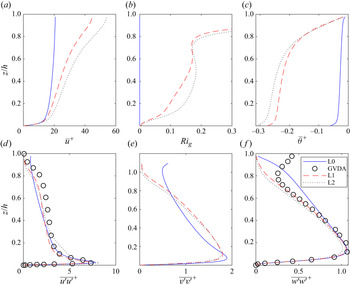
Prior to discussing the kinetic energy density in detail, we explore the main features of the different cases considered in this study. To do so, we consider vertical profiles of horizontally averaged first- and second-order statistics of velocity and temperature (figure 1). The vertical profile of the streamwise mean velocity (figure 1a) shows that the mean streamwise velocity increases with stratification. This is consistent with previous studies on smaller domains (Garg et al. Reference Garg, Ferziger, Monismith and Koseff2000; Armenio & Sarkar Reference Armenio and Sarkar2002; Nieuwstadt Reference Nieuwstadt2005; Taylor et al. Reference Taylor, Sarkar and Armenio2005; Flores & Riley Reference Flores and Riley2011; Donda et al. Reference Donda, van Hooijdonk, Moene, Jonker, van Heijst, Clercx and van de Wiel2015; Atoufi et al. Reference Atoufi, Scott and Waite2019, Reference Atoufi, Scott and Waite2020) and those with comparable domain size (García-Villalba & Álamo Reference García-Villalba and del Álamo2011). However, this increase in mean streamwise velocity is less pronounced in the inner-layer part, where $z/h \lesssim 0.15$ due to the dominance of wall-generated shear over buoyancy (Nieuwstadt Reference Nieuwstadt2005; Taylor et al. Reference Taylor, Sarkar and Armenio2005; García-Villalba & Álamo Reference García-Villalba and del Álamo2011; Atoufi et al. Reference Atoufi, Scott and Waite2020). SS caused by the flux of heat from the top boundary accentuates this increase in mean streamwise velocity moving upwards.

Figure 1.

Vertical profiles of mean flow variables and velocity variances. (a) Mean streamwise velocity, (b) gradient Richardson number, (c) mean temperature, (d) streamwise velocity variance, (e) spanwise velocity variance and (f) wall-normal velocity variance. GVDA refers to digitized data corresponding the case B5b of García-Villalba & Álamo (Reference García-Villalba and del Álamo2011) for closed-channel flow simulation with $Re_\tau =550$, $Ri_\tau =980$, $Pr=0.7$ and fixed bottom and top wall temperatures as boundary conditions for temperature.

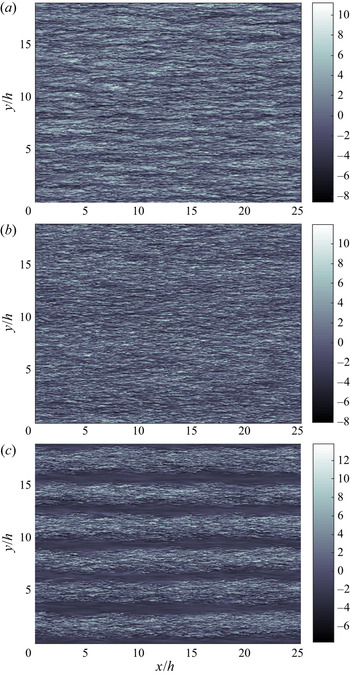
Profiles of streamwise velocity fluctuations in figure 1(d) suggest L0 and L1 have similar near-wall structures (e.g. streaks). The flow pattern in both cases is relatively similar in that spanwise homogeneity of turbulence is achieved. However, in L2, the flow consists of strips of active regions next to quiescent regions, as shown in figure 3. A similar flow structure is seen in the decay and early recovery phase of wall turbulence with surface cooling (Flores & Riley Reference Flores and Riley2011; García-Villalba & Álamo Reference García-Villalba and del Álamo2011; Atoufi et al. Reference Atoufi, Scott and Waite2019). The difference between the patchiness of the flow in L2 and that in our previous studies is that, in L2, the flow does not recover from such spanwise patchiness. This permanent intermittency of the flow in the spanwise direction is due to the balance between two simultaneous sources of SS imposed from the wall and top boundary (figure 1c). The appearance of intermittencies in the form of strips in open-channel turbulence, as opposed to other oblique structures in flows that are bounded by walls at both bottom and at top boundaries (García-Villalba & Álamo Reference García-Villalba and del Álamo2011; Duguet & Schlatter Reference Duguet and Schlatter2013), suggests the importance of the upper boundary condition in the determination of the form and orientation of the intermittent structures. However, further studies are required to understand the relationship between the strips and the oblique structures.

To show the strength of stratification, profiles of gradient Richardson number $Ri_g$ are presented. The $Ri_g$ is defined as

(4.1)\begin{equation} Ri_g=\frac{N^2}{S^2}, \end{equation}

where $N^2=Ri_\tau \partial \bar {\theta }/\partial z$ is the buoyancy frequency and $S^2=(\partial \bar {u}/\partial z)^2 + (\partial \bar {v}/\partial z)^2$. The profiles of $Ri_g$ are shown in figure 1(b). As can be seen, buoyancy becomes more significant over shear and the boundary layer becomes more stable moving upward and as $Ri_\tau$ increases. Consistent with the findings of García-Villalba & Álamo (Reference García-Villalba and del Álamo2011), in the OUL, where $z/h \ge 0.8$, $Ri_g$ acquires values close to the 0.25 stability criterion for both L1 and L2, which signifies strong effects of stratification in the OUL. In the near-wall region $z/h \le 0.15$ shear dominates buoyancy and stratification has minimal effect (Taylor et al. Reference Taylor, Sarkar and Armenio2005; Atoufi et al. Reference Atoufi, Scott and Waite2020).

Mean temperature is roughly constant when temperature is passive as in L0 (figure 1c). For L1 and L2, temperature contributes to the boundary layer dynamics as an active scalar. For both L1 and L2, a strong capping inversion can be seen near the upper boundary of the channel. The vertical gradient of temperature near the bottom wall, in the region $0.05 \lesssim z/h \lesssim 0.2$ increases as $Ri_\tau$ increases.

The velocity variances $\overline {u'u'}$, $\overline {v'v'}$ and $\overline {w'w'}$ for L0, L1 and L2 at stationarity are shown in figure 1(d–f), respectively. In the near-wall region, these profiles are consistent with our earlier observation that, at stationarity, near-wall turbulence is governed mostly by wall-generated mean shear, and stratification plays a relatively minor role. The minimal effect of SS in the near-wall region at stationarity can be observed in figure 1(d,f) where we compared profiles of $\overline {u'^2}$ and $\overline {w'^2}$ with similar profiles from García-Villalba & Álamo (Reference García-Villalba and del Álamo2011) in a closed channel with a different thermal boundary condition (fixed temperature at both walls) and different $Ri_\tau$ ($Ri_\tau =980$). Despite these differences in $Ri_\tau$ and the choice of thermal boundary condition, profiles show similar behaviour in the near-wall region and the dissimilarities become noticeable only in the OUL. The higher values for $\overline {u'u'}$ for L2 in the near-wall region where $z/h \lesssim 0.15$ (figure 1d) in comparison with cases L0 and L1 are due to spanwise patchiness of the flow rather than more intensive streamwise fluctuations (streaks) in the turbulent strips. The upper LGL in L2 is extended to $z/h \approx 0.4$ due to extensive boundary near-wall region growth and shrinkage of the OUL part in L2 (figure 3 side contour plots) relative to L0 and L1. The profiles of $\overline {v'v'}$ and $\overline {w'w'}$ in L2 closely follow L1 in the OUL, where differences become more prominent between L0 and L2.

Stratified turbulence in the OUL is affected by the choice of upper boundary condition. This effect can be understood by comparing wall-normal velocity fluctuations in L0–L2 and closed-channel flow simulations of García-Villalba & Álamo (Reference García-Villalba and del Álamo2011). While free-slip boundary conditions in open-channel flow simulation prevent wall-normal velocity fluctuations with insignificant influence on the streamwise velocity fluctuations (figure 1d), in the closed-channel vertical velocity, fluctuations in $z/h \gtrsim 0.8$ can have values as large as 50 % of the maximum across the channel. In a closed channel, these wall-normal velocity fluctuations maintain downward momentum flux from upper boundary layer and mixing in $z/h \gtrsim 0.8$. In an open channel, however, the impermeability condition at the top boundary prevents vertical momentum flux, which limits the overturning of OUL motions and thus limits vertical mixing.

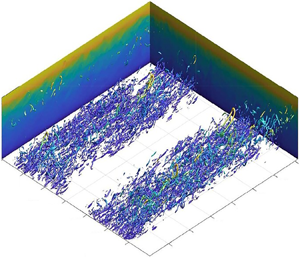
The near-wall streaks spread spanwise direction in L0 and L1 and become patchy in L2, as shown in figure 2. The near-wall vortical structures are dominated by quasi-streamwise vortical structures rather than hairpin-like structures, as shown in figure 3 for L2 in the region where $6{\rm \pi} \leq x/h \leq 8{\rm \pi}$ and $0 \leq y/h \leq 2{\rm \pi}$. Consistent with our previous observations, in which a smaller domain with spanwise domain of size ${\rm \pi}$ has one turbulent strip (Atoufi et al. Reference Atoufi, Scott and Waite2019), the full spanwise length has 6 strips, suggesting that spanwise intermittency has a repeating pattern in the spanwise direction at each ${\rm \pi}$ (figure 2c).

Figure 2.

Streamwise velocity fluctuations ($u'^+$) at $z^+=15$ for (a) L0, (b) L1 and (c) L2.

Figure 3.

Isosurfaces of Q-criterion (second invariant of gradient tensor of fluctuating velocities) for L2 in the region where $6{\rm \pi} \leq x/h \leq 8{\rm \pi}$ and $0 \leq y/h \leq 2{\rm \pi}$, which are coloured by distance from the wall. In the cross-sectional slices, the kinetic energy in the streamwise and spanwise planes is shown. The Q-criterion and total kinetic energy are normalized using their maximum values. The isosurfaces are plotted at the level of 0.01. The colour bar illustrates values of normalized (by the maximum value) total kinetic energy.

4.2. Hierarchy of flow structures

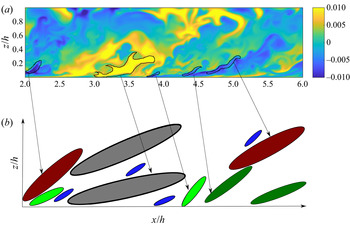
By looking at the energy cascade as a function of specific vertical length scales that are linked to known boundary layer processes, one may have a better understanding of the impact of stable stratification on the energy cascade dynamics. These specific length scales are denoted by $r_z$, and in an energy cascade of wall turbulence can be categorized into four levels. As shown in figure 4(b), the structures in the flow field can be categorized into a hierarchy of discrete bands of $r_z$. The first level of the hierarchy is composed of structures with vertical sizes comparable to the height of the VSL, where $r_z^+=3$. The second level of the hierarchy is composed of flow structures with $r_z^+=15$ to account for BFL sized structures. Therefore, flow structures that are attached to the wall and belong to the second level of the hierarchy might form the BFL. On the other hand, the flow structures that belong to these first two levels and are detached from the wall are small enough to be affected by viscosity and may be involved in viscous effects further away from the wall. The third level of hierarchy is for structures of a size comparable to the height of LGL where $r_z^+=0.14Re_\tau =80$. Finally, the fourth level of hierarchy is composed of the flow structure of the size of the OUL where $r_z^+=0.75Re_\tau =420$. We will come back to the choice of hierarchy of vertical scales in more detail in § 4.4.

Figure 4.

(a) A vertical slice of instantaneous temperature at $tu_\tau ^0/h=13$. (b) Schematic of classifying flow into groups of structures with different vertical scales $r_z$. Blues have the smallest viscosity affected vertical scales. Light greens are structures of a size comparable to the height of the VSL ($r_z^+=3$). Dark greens, red and grey structures represent those with the size of BFL ($r_z^+=15$), LGL ($r_z^+=80$) and OUL ($r_z^5=420$), respectively. The schematic structures in (b) are not scaled representations of those appearing in (a). Smaller structures are actually much smaller than the larger structures shown in (b).

4.3. Kinetic energy

Let us now discuss kinetic energy, which allows us to include the effects of all horizontal modes in the kinetic energy cascade. Before we proceed, it is worth recalling that $\text {ED}(\boldsymbol {k},r_z,z)$ represents energy density for a vertical scale $r_z$ and horizontal wavenumber vector $\boldsymbol {k}$. As we will see, the energy density in small $r_z$ tends to be large, even though the kinetic energy integrated over small scales is relatively small. As a result, we will consider $r_z \text {ED}$ rather than $\text {ED}$, and similarly for terms in the budget, since it gives the energy per octave (or decade) of vertical scale (Hamba Reference Hamba2018). Analogously, we premultiply spectra by horizontal wavenumbers, as is common (Jiménez Reference Jiménez2012; Jiménez Reference Jiménez2013; Cho et al. Reference Cho, Hwang and Choi2018; Atoufi et al. Reference Atoufi, Scott and Waite2020).

4.4. Energy cascade from the perspective of full band of vertical scales

In this section we investigate the full range of values of $r_z$ in the energy density and its budget, before discussing the four representative values in the rest of the manuscript. In this section we consider a smaller domain case C5DC with $L_x/h=2{\rm \pi}$, $L_y/h={\rm \pi}$ and the same parameters as L1 (table 1) because calculations associated with the full range of values of $r_z$ are very expensive on large domains. It was shown in Atoufi et al. (Reference Atoufi, Scott and Waite2020) that the domain size used in C5DC is large enough to capture all essential dominant energy-containing scales of a strongly stable case with similar $Ri_\tau$ as in L1. Since the range of vertical scales present in all cases is $0 \le r_z/h \le 1$ and the domains in C5DC and L1 have the same height, the small domain simulation can inform us about different mechanisms in the energy cascade with respect to a full range of $r_z$ values. Particularly, from the information provided by the full band of $r_z$ in the domain size associated with C5DC, one can identify range of $r_z$ that makes the dominant contribution to the energy density and different terms in its budget in (2.18).

The dependence of $\text {ED}$ on the full range of $r_z$ at different heights is shown in figure 5 for C5DC. The range of $r_z$ values $8 \le r_z^+ \le 20$ corresponds to dominant energy-containing vertical scales which are located in the BFL (figure 5a). Thus, the $r_z^+ \approx 15$ can properly approximate the dominant energy-containing vertical scale. The dominant $r_z$ becomes smaller moving upward from the VSL to the OUL in figure 5(a). In the BFL, where $5 \lesssim z^+ \lesssim 30$, the spectrum is concentrated around the line shown in figure 5(a). The peak in the premultiplied energy density takes place at slightly smaller $r_z$ as the wall distance increases. Except for the OUL, all of these peaks correspond to BFL size $r_z$.

Figure 5.

Premultiplied energy density ($r_z \sum _{\boldsymbol {k}}\text {ED}$) in C5DC for (a) different $r_z$, summed over all $\lambda _x$ and $\lambda _y$ at different heights and (b) premultiplied energy density at vertical locations in VSL, BFL, LGL and OUL for all vertical scales. The blue dashed dotted line in (a) shows the line $2.4 + 0.2 \ln {r_z^+}$.

Although we assumed a hierarchy of vertical scales in our analysis, the choice of this hierarchy needs more discussion. To do so, one can employ (2.19) and figure 5(b). The choice of $r_z^+=3$, $r_z^+=15$, $r_z^+=80$ and $r_z^+=420$ serves as representative values for the different regions (I, II, III, IV) in figure 5(b). In region I: $r_z^+ \in [0,5)$, II: $r_z^+ \in [5,30)$, IV: $r_z^+ \in [30,100)$ and in IV: $r_z^+ \in [100,Re_\tau ]$. Except for the OUL (5b), the BFL size $r_z$ with $8 \lesssim r_z^+ \lesssim 20$ is the most energetic vertical scale. In the VSL, $r_z \approx 15$ are dominant vertical scales whereas in the BFL and LGL $r_z^+ \approx 8$ and $r_z^+ \approx 10$, are the dominant vertical scales, respectively. In the OUL, very small $r_z$ of a size comparable to the height of the VSL are dominant. The energy density is less skewed toward large vertical scales by increasing $z^+$ as can be seen in figure 5(b). This finding, along with our conclusion from figure 7 in which dominant energy-containing $\lambda _x$ become larger as $r_z$ increases, suggests that energy-containing structures become elongated but thinner moving upward. This finding suggests an explanation for the appearance of thin, layered, pancake-like structure in the outer-layer part of a strongly stably stratified open-channel flow (Atoufi et al. Reference Atoufi, Scott and Waite2019).

4.5. Energy cascade from the perspective of hierarchy of vertical scales

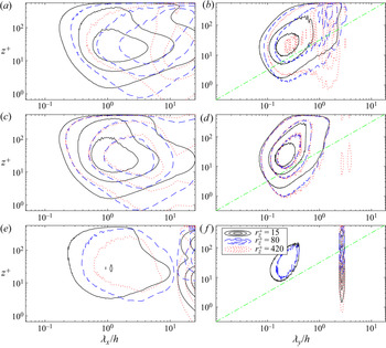
Figure 6 shows the dependence of $\text {ED}$ upon horizontal and vertical scales and also how the energy distribution is changed by stratification. We first discuss the dependence of energy density upon streamwise scales $\lambda _x$ and height for different $r_z$ and stratifications. To do so, $\text {ED}$ (2.14) is summed over $\lambda _y$ and contour plots of the result are shown in figure 6(a,c,e) which correspond to L0, L1 and L2, respectively. In L0 and L1, $\text {ED}$ is concentrated at larger $\lambda _x$ as $r_z$ increases (figure 6a,c). Moreover, by comparing figure 6(a,c) for $r_z^+=15$, one can say that the $\lambda _x$ spectrum gets narrower by increasing the stability of the boundary layer (increasing $Ri_\tau$). For example, the contour lines in L0 for $r_z^+=15$, which contain less than 0.15 of the $\text {ED}$ maximum, do not become closed for $\lambda _x \simeq L_x$. In L1 (for $r_z^+=15$), contour lines referring to 0.15 of $\text {ED}$ maximum become closed for $\lambda _x \simeq L_x$. In L2, the most energetic streamwise scales ($\lambda _x/h \sim 1$) are suppressed and the largest $\lambda _x$ become more active compared with L1

Figure 6.

Premultiplied energy density ($\text {ED}$) for (a,c,e) streamwise ($r_z k_x \sum _{k_y}{\text {ED}}$) and (b,d,f) spanwise ($r_z k_y \sum _{k_x}{\text {ED}}$) wavelengths. Panels (a,b), (c,d) and (e,f) respectively refer to L0, L1 and L2. Contours are plotted at 0.15, 0.45 and 0.75 of the maxima of corresponding spectra. The dashed-dotted green straight line in log–log plots in (b,d,f) shows the power-law relation between non-dimensional spanwise wavelengths and height as $\log \lambda _y=1.3+\log z$.

In L0, for $r_z$ the size of the LGL with $r_z^+=80$ (figure 6a), the largest $\text {ED}$ belongs to large structures with size in the range $\lambda _x/h$ from 3 to 10, consistent with García-Villalba & Álamo (Reference García-Villalba and del Álamo2011). These structures reside in the BFL and extend into the OUL, showing that structures with this vertical scale link viscous regions to the OUL. Thus, the third level of hierarchy bridges energy-containing scales of the size $\lambda _x/h \sim 1$ in the BFL to less energetic scales of the size $\lambda _x/h \sim L_x/h$ in the OUL. In contrast, such a link between streamwise scales in the inner and OULs by vertical structures of the size as the height of LGL (figure 6(a), inclined dashed blue contour lines) is suppressed in stratified cases L1 and L2 (figure 6d,f). In L2, $\text {ED}$ resides mostly in the largest $\lambda _x$ of the size of $L_x$. Moreover, in the most stratified case L2, the structures with a vertical size of $r_z^+=80$ do not reach the wall.

Now we discuss the dependence of energy density upon spanwise scales $\lambda _y$ and height for different $r_z$ and different simulations. To do so, $\text {ED}$ is summed over $\lambda _x$, and contour plots of results are shown in figure 6(b,d,f) which correspond to L0, L1 and L2, respectively. The energy-containing spanwise scales are smaller than the energy-containing streamwise scales for all $r_z$. The dependence of energy-containing $\lambda _y$ upon $r_z$ is much weaker than streamwise scales. The energy density spectrum as a function of $\lambda _y$ and height concentrates approximately around the line $\lambda _y \sim z$ in the logarithmic region. The approximately linear dependence of $\lambda _y$ on the distance from the wall signifies the role of the LGL in the formation of the attached eddies (Cho et al. Reference Cho, Hwang and Choi2018; Hwang & Bengana Reference Hwang and Bengana2016). The symmetry of spanwise scales around the line $\lambda _y \sim z$ is preserved for all energetic $r_z$, suggesting that energy-containing spanwise scales in the LGL are linearly dependent upon the distance from the wall. The similarity in behaviour of energy-containing spanwise scales upon height also suggests there is a self-similar process affecting all spanwise scales (i.e. self-sustaining process). All of the $r_z$ scales are most energetic at $z^+ \approx 15$.

In L2, there is a narrow band in which the size of energetic spanwise scales is almost constant with respect to height and for all $r_z$. This $\lambda _y/h \approx 3$ ($\lambda _y^+ \approx 1700$) associated with this band contains one turbulent strip and one quiescent region (figure 3). Since there are six strips, the wavelength is $\lambda _y=L_y/6$ and therefore $\lambda _y/h={\rm \pi} \approx 3$ corresponds to the wavelength of the strip. Moreover, energetic spanwise scales $\lambda _y/h \sim 0.2$ at $z^+ \in [10 - 100]$ for L2 are dominated by $r_z$ of the size of the BFL and LGL height. These energetic scales are responsible for sustaining turbulence in the active regions (turbulent strips). The footprint of the OUL size structures in the BFL is not observed in L2 for energy-containing spanwise scales. The presence of turbulent strips in the near-wall region without a footprint of $r_z^+=420$ sized structures suggests that near-wall turbulence in an SBL can be autonomously sustained even without interacting with OUL sized structures with vertical size comparable to $h$, similar to unstratified cases (Jiménez & Pinelli Reference Jiménez and Pinelli1999).

The magnitude of premultiplied $\text {ED}$ for all levels in the hierarchy is shown in figure 7 for a single stratification, L1. This case is chosen since stratification effects on turbulence are shown to be strong earlier in the surface cooling process (Atoufi et al. Reference Atoufi, Scott and Waite2019, Reference Atoufi, Scott and Waite2020). For this case, once turbulence acquires stationarity, spanwise homogeneity of turbulence is maintained. As shown, $r_z^+=15$ is the most energetic vertical scale among the $r_z$ discussed here, which corresponds to structures of vertical size comparable to the height of the BFL. The second, third and fourth largest $r_z\text {ED}$ correspond to $r_z^+=3$, $r_z^+=80$, $r_z^+=420$. Moreover the largest premultiplied $\text {ED}$ in the OUL is associated with the small viscous scales, $r_z^+=3$. As seen in figure 7(a,b), the energetic streamwise and spanwise scales are much larger than the Kolmogorov scales everywhere, suggesting that the Kolmogorov scales are smaller than the horizontal energy-containing scales, even for the smallest vertical scales of the size comparable to the height of VSL with $r_z^+=3$.

Figure 7.

Premultiplied energy density for (a,c,e,g) streamwise ($r_z k_x \sum _{k_y}{\text {ED}}$) and (b,d,f,h) spanwise ($r_z k_y \sum _{k_x}{\text {ED}}$) wavelengths for L1. Panels (a,b), (c,d), (e,f) and (g,h) respectively refer to $r_z^+=3$, $r_z^+=15$, $r_z^+=80$ and $r_z^+=420$. The dashed-dotted yellow line in (a,b) is the profile of $30 \eta (z)/h$ where $\eta =(\nu ^3/\epsilon )^{(1/4)}$ refer to Kolmogorov scales.

4.6. Nonlinear energy transfer

In this section, the nonlinear transfer of $\text {ED}$ is discussed. We start by analysing the dependence of $\text {TR}$ on $r_z$ only by summing $\text {TR}$ over all $\lambda _x$ and $\lambda _y$, as shown in figure 8. We also include the conventional horizontally averaged turbulence transport $T$ in the TKE budget (Garg et al. Reference Garg, Ferziger, Monismith and Koseff2000; Armenio & Sarkar Reference Armenio and Sarkar2002; Taylor et al. Reference Taylor, Sarkar and Armenio2005; Huang & Bou-Zeid Reference Huang and Bou-Zeid2013; Flores & Riley Reference Flores and Riley2018; Atoufi et al. Reference Atoufi, Scott and Waite2019, Reference Atoufi, Scott and Waite2020) to show how closely $\text {TR}$ at each $r_z$ follows $T$.

Figure 8.

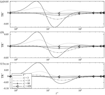
Premultiplied nonlinear transfer ($r_z \sum _{\boldsymbol {k}}\text {TR}$) for different $r_z$, summed over all $\lambda _x$ and $\lambda _y$, for (a) L0, (b) L1 and (c) L2. Here, $r_z=0$ refers to horizontally averaged TKE transport and $T^+$ refers to turbulence transport in horizontally averaged TKE budget normalized by $Re_\tau$ (Atoufi et al. Reference Atoufi, Scott and Waite2019, Reference Atoufi, Scott and Waite2020).

The value of $\text {TR}$ summed over all horizontal wavelengths is much smaller for large vertical scales $r_z^+=420$ and $r_z^+=80$ than small vertical scales $r_z^+=15$ and $r_z^+=3$ across the channel height. The $\text {TR}$ term for $r_z^+=15$ is positive in the VSL and negative everywhere else, while $\text {TR}$ for $r_z^+=3$ is positive across the channel height. For a particular $r_z$ and $z$, the sign of $\text {TR}$ summed over all horizontal wavelengths indicates whether energy density is transferred out of (negative) or into (positive) that particular $z$. By comparing the profile for the dominant $r_z$ with the TKE transport term $T$ one may acquire further insight into the transport of ED for the dominant $r_z$ toward or away from the wall. In the near-wall region, the positive and negative transfers are consistent with ejections and sweeps, respectively. By comparing profiles of premultiplied $\text {TR}$ (summed over horizontal wavenumbers) for different $r_z$ with the TKE transport term $T$ (Atoufi et al. Reference Atoufi, Scott and Waite2020), it is clear that ejections in the lower part of VSL are controlled by eddies with a vertical size comparable to the height of the VSL for the different stratifications considered here. Thus, motions of larger eddies of the size of the buffer, logarithmic and OULs do not contribute to transport in the VSL. However, in the BFL and above, all $r_z$ contribute to $\text {TR}$.

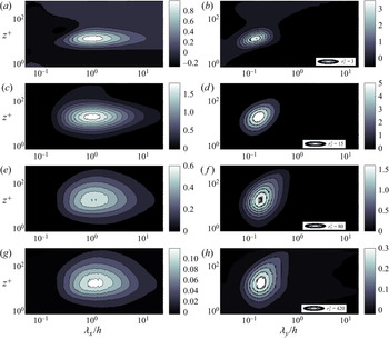
The premultiplied spectra of $\text {TR}$ are shown in figure 9 for L1. We first discuss the dependence of $\text {TR}$ upon $\lambda _x$ and $r_z$ as shown in figure 9(a,c,e,g). The small streamwise scales with $\lambda _x/h \sim 0.2$ contribute to the largest positive values of premultiplied $\text {TR}$ for $r_z^+=3$ and 15. The vertical scales with $r_z^+=3$ contribute more to positive $\text {TR}$, as also shown in figure 8. In the VSL and lower BFL, the streamwise scales $\lambda _x/h$ from $0.2$ to $3$ are dominant in positive $\text {TR}$ (figure 9a). In the BFL and aloft, the negative $\text {TR}$ is associated with $1 \lesssim \lambda _x/h \lesssim 10$ (figure 9a,c,e,g).

Figure 9.

Premultiplied nonlinear transfer of energy density ($\text {TR}$) for (a,c,e,g) streamwise ($r_z k_x \sum _{k_y}{\text {TR}}$) and (b,d,f,h) spanwise ($r_z k_y \sum _{k_x}{\text {TR}}$) wavelengths for L1. Panels (a,b), (c,d), (e,f) and (g,h) respectively refer to $r_z^+=3$, $r_z^+=15$, $r_z^+=80$ and $r_z^+=420$.

Insights from nonlinear transfer for different vertical scales may improve our understanding of the inner and OUL interactions. Figure 9(a,c) suggests that, for $r_z^+=3$ and $r_z^+=15$ in the VSL and lower part of BFL, $\text {ED}$ transfers into small streamwise scales ($\lambda _x/h < 1$) and out of larger streamwise scales ($\lambda _x/h > 1$) at the same height and aloft as shown in figure 9(a,c). For a given $r_z$, this energy transfer occurs from vertical scales greater than or equal to $r_z^+=80$, since for $r_z^+=420$ the transfer is mostly negative (figure 8b). For $r_z^+=80$ and $r_z^+=420$ (figure 9e,g) $\text {TR}$ is primarily negative and thus $\text {TR}$ mostly transfers out of such $r_z$. Also, for $r_z^+=420$ the $\text {ED}$ at $\lambda _x/h \lesssim 1$ is positive, which shows such large $r_z$ contributes to transferring energy into $\lambda _x/h \lesssim 1$ wavelengths in the upper VSL. The large streamwise scales with $\lambda _x \sim L_x$ for OUL size vertical scales ($r_z^+=420$, figure 9g) contribute slightly to positive transfer, which penetrates down to the VSL. Large vertical scales with $r_z^+=420$ are tall enough ($r_z=0.75h$) to influence the whole boundary layer, so they can contribute to the positive transfer of $\text {ED}$ for the largest streamwise scales in the VSL. The negative transfer is more pronounced for $\lambda _x/h \sim 3$ regardless of $r_z$ (and also stratification; not shown).

Now we discuss the dependence of $\text {TR}$ upon $\lambda _y$ and $r_z$, as shown in figure 9(b,d,f,h). Generally, transfer takes place at spanwise scales that are an order of magnitude smaller than streamwise scales, consistent with studies of unstratified channel flows (Cho et al. Reference Cho, Hwang and Choi2018). However, the maximum absolute values of transfer rate by spanwise scales are larger than those in streamwise scales. The largest values of positive and negative premultiplied $\text {TR}$ are due to $r_z^+=3$ and $r_z^+=15$ respectively. Similar to the $\text {ED}$ spectra in figure 7, $\text {TR}$ concentrates around a line $\lambda _y \sim z$ in the logarithmic region for $r_z^+ > 3$, which strongly suggests that the LGL consists of self-similar attached eddies (Hwang Reference Hwang2015). For $r_z^+=3$ (figure 9b) the VSL and lower BFL contain small spanwise scales with $\lambda _y/h \sim 0.2$ that contribute to largest positive $\text {TR}$. For $r_z^+=3$, the upper BFL and lower LGL contains negative transfer. Thus for $r_z^+=3$, the $\text {ED}$ is transferred into $\lambda _y/h \sim 0.2$ in the upper VSL and lower BFL and out of slightly smaller scales in upper BFL and lower LGL. For $r_z^+>3$ in figure 9(d,f,h) the $\text {ED}$ is mostly transferred out of small spanwise scales with $\lambda _y/h \sim 0.2$ in the BFL and $\lambda _y \sim z$ in the LGL to other $\lambda _y$. For $r_z^+=80$ and $420$, $\text {ED}$ is transferred from $\lambda _y/h \lesssim 0.2$ even in the VSL. The nonlinear transfer for $r_z^+ > 3$ is dominated by in-plane triad interactions (not shown for brevity).

4.7. Turbulence production

In this section, the production of $\text {ED}$ is discussed. The spectra of turbulence production ($\text {SP}$) are shown in figure 10 for all simulations. The dependences of $\text {SP}$ on streamwise scales, vertical scales, distance from the wall and stratification are shown in figure 10(a,c,e). The $\lambda _x$ scales of the size of the channel height ($\lambda _x/h \approx 1$) centred at the BFL are the most productive scales for premultiplied $\text {ED}$. In L0 and L1, the less energetic streamwise scales carrying at least 0.1 of $\text {SP}$ maxima become smaller with increasing $Ri_\tau$. By comparing figure 10(a,c,e) and figure 6, one can say that less energetic structures in the OUL of vertical size $r_z^+=80$ and $r_z^+=420$ are large with $\lambda _x/h \ge 10$ and penetrate the buffer region, suggesting they are inactive eddies as they only slightly contribute to production.

Figure 10.

Premultiplied shear production ($\text {SP}$) for (a,c,e) streamwise ($r_z k_x \sum _{k_y}{\text {SP}}$) and (b,d,f) spanwise ($r_z k_y \sum _{k_x}{\text {SP}}$) wavelengths. Panels (a,b), (c,d) and (e,f) respectively refers to L0, L1 and L2. Contours are plotted at 0.15, 0.45 and 0.75 of the maxima of corresponding spectra.

The dependence of $\text {SP}$ on spanwise scales is shown in figure 10(b,d,f). The most productive spanwise scales for premultiplied $\text {ED}$ in the BFL are of the size $\lambda _y/h \simeq 0.2$ ($\lambda _y ^ + \simeq 100$) for all $r_z$ and regardless of stratification. The scale $\lambda _y ^ + \simeq 100$ is consistent with near-wall streak spacing for unstratified channels (Jiménez & Moin Reference Jiménez and Moin1991) and thus shows turbulence production in the near-wall region is strongly linked to near-wall streaks. Turbulence producing spanwise scales with vertical size of the logarithmic and OULs are similar when $\text {SP}$ is normalized using corresponding maximum values. Thus, turbulence producing spanwise scales with the vertical size of the logarithmic and OULs are similar and SS is in favour of making this coupling even stronger, so that contour lines in figure 10(d) for $r_z^+=80$ follow those for $r_z^+=420$ even more closely than in figure 10(b). In L2, $\lambda _y/h \approx 3$ are spanwise scales containing an active region next to a quiescent region at which production is slightly negative. The similarity between turbulence producing spanwise scales ($\lambda _y$ in the $\text {SP}$) in L0, L1 and L2 can be seen in figure 10(b,d,f). Figure 10(f) shows that, in L2, the widest turbulence producing structure (active region) is of spanwise size comparable to $h$. The presence of $\text {SP}$ at $\lambda _y/h \approx 3$ in L2 explains why strips appear with a width comparable to $3h$.

The magnitude of $\text {SP}$ for all levels in the hierarchy is shown in figure 11 for a single stratification, L1. Turbulence production takes place at all $r_z$. The vertical scale $r_z^+=15$ (figure 11c) contributes to the premultiplied $\text {SP}$ maximum, and the maximum premultiplied $\text {SP}$ occurs in the BFL for all $r_z$ considered here for L1. The vertical scale with $r_z^+=3$ (figure 11a), $r_z^+=80$ (figure 11e) and $r_z^+=420$ (figure 11g) contain other relatively large productions for streamwise scales. The largest value of $\text {SP}$ associated with $\lambda _y$ is three times larger (figure 11b,d,f,h) than the largest production associated with $\lambda _x$ for all $r_z$ (and also stratification regimes). In fully developed cases (L0 and L1) and also in the active regions of L2 (results for L0 and L2 are not shown here), $\text {SP}$ in the BFL for horizontal and vertical scales shows a sustained kinetic energy injection associated with mean shear into all streamwise scales, all vertical scales and spanwise scales between 0.1 and 1. This finding is consistent with a scale-by-scale budget of the structure function in Casciola et al. (Reference Casciola, Gualtieri, Benzi and Piva2003) for unstratified shear layer turbulence.

Figure 11.

Premultiplied shear production ($\text {SP}$) for (a,c,e,g) streamwise ($r_z k_x \sum _{k_y}{\text {SP}}$) and (b,d,f,h) spanwise ($r_z k_y \sum _{k_x}{\text {SP}}$) wavelengths for L1. Panels (a,b), (c,d), (e,f) and (g,h) respectively refer to $r_z^+=3$, $r_z^+=15$, $r_z^+=80$ and $r_z^+=420$.

4.8. Viscous effects

The premultiplied $\text {VD}$ spectra are shown in figure 12 for L1. Generally, the vertical scale $r_z^+=3$ contains the maximum absolute values of viscous effects (premultiplied $\text {VD}$) among the $r_z$ considered here. The dependence of $\text {VD}$ on $\lambda _x$ and $r_z$ are shown in figure 12(a,c,e,g). The magnitude of the viscous term decreases with increasing vertical scale. The large values of $\text {VD}$ (magnitude greater than 0.1) are negative in the near-wall region for $r_z^+=3$ and $r_z^+=15$ (figure 12a,b). This negative $\text {VD}$ suggests that dissipation of $\text {ED}$ in the near-wall region is associated with small $r_z$, as expected. As opposed to production ($\text {SP}$), the spectral distribution of viscous effects among different streamwise scales is more sensitive to $r_z$. The $\text {VD}$ spectra for $r_z^+=3$ and $r_z^+=15$ are different than those with $r_z^+=80$ and $r_z^+=420$. Viscous effects take place at larger streamwise $\lambda _x$ as $r_z$ increases. Also, viscous effects spread out over a wider range of $\lambda _x$ as $r_z$ increases. The dependence of the viscous effects on spanwise scale are shown in figure 12(b,d,f,h). The most viscosity affected $\lambda _y$ is much smaller than the corresponding $\lambda _x$. For $r_z^+=3$ and $r_z^+=15$ $\text {VD}$ is negative almost anywhere across channel height for all $\lambda _y$ whereas for $r_z^+=80$ and $r_z^+=420$ the $\text {VD}$ is positive, but small, in the VSL. By comparing both $\lambda _x$ and $\lambda _y$ contours, we see that the strongest viscous effects take place in the lower BFL. The viscous term $\text {VD}$ for both $\lambda _x$ and $\lambda _y$ are similar for $r_z$ of size comparable to the height of LGL and OUL.

Figure 12.

Premultiplied viscous effects ($\text {VD}$) for (a,c,e,g) streamwise ($r_z k_x \sum _{k_y}{\text {VD}}$) and (b,d,f,h) spanwise ($r_z k_y \sum _{k_x}{\text {VD}}$) wavelengths for L1. Panels (a,b), (c,d), (e,f) and (g,h) respectively refer to $r_z^+=3$, $r_z^+=15$, $r_z^+=80$ and $r_z^+=420$.

Viscous diffusion in the VSL is positive in the horizontally averaged TKE budget, as discussed in Atoufi et al. (Reference Atoufi, Scott and Waite2020). The $\text {VD}$ summed over wavelengths is shown in figure 13. As can be seen, the $\text {VD}$ term corresponds to the summation of viscous dissipation and diffusion, which are total effects of viscosity in a horizontally averaged TKE budget. Thus, small positive $\text {VD}$ for $r_z^+=80$ and $r_z^+=420$ in the VSL is associated with viscous diffusion since dissipation is negative.

Figure 13.

Premultiplied viscous term ($r_z \sum _{\boldsymbol {k}}\text {VD}$) for different $r_z$, summed over all $\lambda _x$ and $\lambda _y$, for (a) L0, (b) L1 and (c) L2. The $\epsilon ^+$ and $D^+$ refers to turbulence dissipation and diffusion, respectively in horizontally averaged TKE budget normalized by $Re_\tau$ (Atoufi et al. Reference Atoufi, Scott and Waite2019, Reference Atoufi, Scott and Waite2020).

Note that positive values of $\text {VD}$ come from inter-plane viscous effects since $\text {VD}_i$ is directly related to ($-\text {ED}$) which is negative ((2.27)). For $r_z$ of the size of the LGL and OUL, $\text {VD}$ becomes positive at small wavelengths, signifying dominance of inter-plane viscous effects at such scales. These positive $\text {VD}$ occur in the lower part of the VSL, suggesting that the role of such tall vertical structures is to actually intensify $\text {ED}$. This intensification of $\text {ED}$ in the lower part of the VSL takes place at $\lambda _x/h \approx 1$ and $\lambda _y/h \approx 0.2$, which correspond to the scales contributing to maximum $\text {SP}$. Thus, part of the $\text {ED}$ generation in the lower part of the VSL is a result of inter-plane viscous effects. We will discuss the importance of the positive $\text {VD}$ shortly. The magnitude of the $\text {VD}_i$ is much smaller than $\text {VD}$ at all scales (not shown for brevity) and therefore the $\text {VD}$ is primarily controlled by inter-plane viscous effects, and the role of in-plane viscous effects is secondary.

Now we discuss the importance of positive $\text {VD}$. It has been discussed by Atoufi et al. (Reference Atoufi, Scott and Waite2020) that pressure work, similar to unstratified channel flows, is a crucial mechanism for transporting turbulence from the lower VSL, where the transport term in the horizontally averaged TKE budget is small. However, pressure work requires sustainable velocity fluctuation to actively transfer TKE to the upper VSL, where transfer terms can distribute TKE to the rest of the channel. An important question is which mechanism in the viscous region, where production is also small due to wall impermeability, can provide sustainable velocity fluctuations? As discussed, inter-plane viscous interactions among scales of the size of the LGL and OUL seem to be a plausible answer. The nonlinear transfer, production and buoyancy (will be discussed shortly) terms are small compared with viscous effects in the lower VSL, similar to unstratified channel flows (Jiménez Reference Jiménez1999; Bernardini, Pirozzoli & Orlandi Reference Bernardini, Pirozzoli and Orlandi2014; Atoufi et al. Reference Atoufi, Scott and Waite2020).

4.9. Buoyancy destruction

Buoyancy is not a dominant mechanism in the budget of horizontally averaged TKE for the SBL (Nicholl Reference Nicholl1970; Arya Reference Arya1975; Van Buren et al. Reference Van Buren, Williams and Smits2017; Shah & Bou-Zeid Reference Shah and Bou-Zeid2019; Atoufi et al. Reference Atoufi, Scott and Waite2020). Similarly, it is not a dominant mechanism in the budget of $\text {ED}$. However, to identify the range of scales that are most affected by buoyancy, we discuss BD spectra in this section for L1.

The dependence of $\text {BD}$ on $\lambda _x$ is shown in figure 14(a,c,e,g). The premultiplied $\text {BD}$ is concentrated in the LGL and is dominated by $r_z^+=15$. As $r_z$ increases, $\text {BD}$ effects extend deeper down in the boundary layer and involves larger $\lambda _x$. The range of buoyancy affected $\lambda _x/h$ extends from 0.1 to 10 for $r_z^+=15$. As $r_z^+$ increases to $420$, the range of buoyancy affected $\lambda _x/h$ extends from 1 to $L_x$. The dependence of $\text {BD}$ on $\lambda _y$ is shown in figure 14(b,d,f,h). The $\lambda _y$ spectra are narrower than the $\lambda _x$ spectra, similar to other terms in $\text {ED}$ budget discussed so far. As $r_z$ increases, $\text {BD}$ involves larger $\lambda _y$. The ranges of buoyancy affected $\lambda _y/h$ scales extend from $0.2$ to 1 for $r_z^+=15$ and from $0.2$ to 10 for $r_z^+=420$.

Figure 14.

Premultiplied buoyancy term ($\text {BD}$) for (a,c,e,g) streamwise ($r_z k_x \sum _{k_y}{\text {BD}}$) and (b,d,f,h) spanwise ($r_z k_y \sum _{k_x}{\text {BD}}$) wavelengths for L1. Panels (a,b), (c,d), (e,f) and (g,h) respectively refer to $r_z^+=3$, $r_z^+=15$, $r_z^+=80$ and $r_z^+=420$.

By comparing $\text {BD}$ and $\text {SP}$ spectra for L1 (figures 14 and 11), one might say that the range of scales that is affected by buoyancy includes all scales that contribute to turbulence production. This range of buoyancy affected scales is expected since part of the kinetic energy injected by $\text {SP}$ is converted to potential energy by $\text {BD}$. But there are large scale $\lambda _x/h \sim L_x/h$ and $\lambda _y/h \gtrsim 1$ for all $r_z$ that contribute to $\text {BD}$ but not $\text {SP}$. Also, the maximum of $\text {BD}$ for streamwise scales is centred farther from the wall compared with $\text {SP}$.

Although buoyancy is not a dominant mechanism in the energy budget for reasons explained below, it imposes an additional restriction on the computational domain size. As can be seen in figure 14 for $r_z^+=420$, buoyancy activates large spanwise scales that contribute to $\text {BD}$ more than for $\text {SP}$. The SS is in favour of suppressing large non-productive vertical scales by widening their corresponding spanwise $\lambda _y$ and elongating their $\lambda _x$ (figure 14).