1. Introduction
Wind turbine wakes substantially reduce power output and increase fatigue loads on downstream turbines in wind farms (Stevens & Meneveau Reference Stevens and Meneveau2017; Porté-Agel et al. Reference Porté-Agel, Bastankhah and Shamsoddin2020). Measurements show wake-induced power losses of up to 40 %, and fatigue load increases of up to 80 % (Barthelmie et al. Reference Barthelmie2007; Wang et al. Reference Wang2023), with extreme cases reaching 60–80 % power loss (El-Asha et al. Reference El-Asha, Zhan and Iungo2017). Wake-induced performance reductions depend on various factors (Chamorro & Porté-Agel Reference Chamorro and Porté-Agel2010), such as atmospheric conditions, turbine spacing and operational parameters. One frequently overlooked factor is wind turbine blade design. Our recent work demonstrates that blade spanwise axial force distribution, which is often ignored in analytical wake models, significantly impacts velocity recovery and dynamics of coherent flow structures (Dong et al. Reference Dong, Qin, Li and Yang2023). This finding suggests the potential of designing blades for optimal wind farm performance, extending beyond conventional turbine-level approaches (Burton et al. Reference Burton, Jenkins, Sharpe and Bossanyi2011). However, realising such advancements requires a fundamental understanding of how blade design affects wake dynamics at the array level. Field studies of this potential are challenging due to limited availability of blade data. At the first step, in this work, we use large-eddy simulations (LES) coupled with an actuator surface (AS) model to study how blade designs affect wake flow mechanisms in tandem wind turbines.
Wind turbine wakes are typically divided into near-wake and far-wake regions. The near wake features coherent structures such as helical tip vortices, blade root vortices and hub vortex (Widnall Reference Widnall1972; Posa et al. Reference Posa, Broglia and Balaras2021). These structures are sensitive to blade design (Dong et al. Reference Dong, Qin, Li and Yang2023) and control actions (Brown et al. Reference Brown, Houck, Maniaci, Westergaard and Kelley2022). In the far wake, wake meandering emerges as the dominant phenomenon. This low-frequency, large-scale lateral/vertical wake displacement enhances momentum entrainment at the wake boundary, accelerating flow recovery (Larsen et al. Reference Larsen, Madsen, Thomsen and Larsen2008; Madsen et al. Reference Madsen, Larsen, Larsen, Troldborg and Mikkelsen2010; Foti et al. Reference Foti, Yang, Guala and Sotiropoulos2016; Yang & Sotiropoulos Reference Yang and Sotiropoulos2019a ). Wake meandering originates from two mechanisms. (i) Inflow large-eddy advection – the wake is often treated as a passive scalar advected by inflow large-scale turbulent eddies (Larsen et al. Reference Larsen, Madsen, Thomsen and Larsen2008; Trujillo et al. Reference Trujillo, Bingöl, Larsen, Mann and Kühn2011; Espana et al. Reference Espana, Aubrun, Loyer and Devinant2012; Porté-Agel et al. Reference Porté-Agel, Bastankhah and Shamsoddin2020), underpinning the dynamic wake meandering model (Larsen et al. Reference Larsen, Madsen, Thomsen and Larsen2008; Keck et al. Reference Keck, de Maré, Churchfield, Lee, Larsen and Aagaard Madsen2014). (ii) Wake shear layer instability – the meandering dynamics mimics bluff-body vortex shedding (Medici & Alfredsson Reference Medici and Alfredsson2006; Medici & Alfredsson Reference Medici and Alfredsson2008; Okulov et al. Reference Okulov, Naumov, Mikkelsen, Kabardin and Sørensen2014; Foti et al. Reference Foti, Yang, Campagnolo, Maniaci and Sotiropoulos2018a ; Dong et al. Reference Dong, Qin, Li and Yang2023). Interactions between the hub-vortex-dominated inner wake and the tip-vortex-governed shear layer can trigger and amplify meandering (Kang et al. Reference Kang, Yang and Sotiropoulos2014; Foti et al. Reference Foti, Yang and Sotiropoulos2018b ). This mechanism is supported by linear stability analyses (Iungo et al. Reference Iungo, Viola, Camarri, Porté-Agel and Gallaire2013; Li et al. Reference Li, Dong and Yang2022) and experiments (Biswas & Buxton Reference Biswas and Buxton2024). Our recent LES studies (Dong et al. Reference Dong, Qin, Li and Yang2023) demonstrate the effects of blade design on wake meandering, that root-loaded designs, with high load near blade root, increase meandering amplitudes.
Wake evolution is strongly influenced by inflow conditions. The wake dynamics of a stand-alone wind turbine has been extensively studied under both laminar and turbulent inflows (Stevens & Meneveau Reference Stevens and Meneveau2017; Yang & Sotiropoulos Reference Yang and Sotiropoulos2019a ; Porté-Agel et al. Reference Porté-Agel, Bastankhah and Shamsoddin2020; Wu et al. Reference Wu, Lin and Chang2020). In wind farms, key factors influencing turbine inflow conditions include atmospheric stability (Syed et al. Reference Syed, Mann, Platis and Bange2022), terrain effects (Yang et al. Reference Yang, Pakula and Sotiropoulos2018) and upstream wakes (Andersen et al. Reference Andersen, Sørensen and Mikkelsen2017). Inflow turbulence accelerates wake recovery (Li et al. Reference Li, Murata, Endo, Maeda and Kamada2016; Wu et al. Reference Wu, Lin and Chang2020) and alters vortex structure evolution (Yang et al. Reference Yang, Hong, Barone and Sotiropoulos2016). Gambuzza & Ganapathisubramani (Reference Gambuzza and Ganapathisubramani2023) experimentally compared Kolmogorov-like and non-Kolmogorov-like turbulent inflows, demonstrating that low-frequency fluctuations in non-Kolmogorov flows are less effective in promoting momentum entrainment across wake boundaries. Through systematic LES with synthetic turbulence generation (Mann Reference Mann1998), Li et al. (Reference Li, Zhang, Li and Yang2024) quantified distinct roles of inflow turbulence parameters, showing that turbulence intensity primarily determines the onset location of wake recovery, while the integral length scale primarily controls the scaling exponents of wake recovery.
An important metric characterising wake meandering is the Strouhal number
 $\textit{St} = f U_{\textit{hub}}/D$
, where
 $f$
,
 $U_{\textit{hub}}$
and
 $D$
represent the meandering frequency, incoming wind speed at hub height, and rotor diameter, respectively. Wake meandering occurs across a range of Strouhal numbers in experiments and simulations. Medici & Alfredsson (Reference Medici and Alfredsson2006) reported
 $0.12 \lt St \lt 0.25$
in wind tunnel tests; later work showed its dependence on tip speed ratio (TSR) and thrust coefficient (Medici & Alfredsson Reference Medici and Alfredsson2008). For an axial-flow hydrokinetic turbine, Chamorro et al. (Reference Chamorro, Hill, Morton, Ellis, Arndt and Sotiropoulos2013) identified
 $0.33 \lt St \lt 0.40$
, while Barlas et al. (Reference Barlas, Buckingham and van Beeck2016) observed a dominant frequency near
 $\textit{St} \approx 0.25$
under low-turbulence conditions. Heisel et al. (Reference Heisel, Hong and Guala2018) summarised
 $\textit{St}$
values (0.1–0.4) for shear-layer-induced meandering. This aligns with linear stability analyses by Mao & Sørensen (Reference Mao and Sørensen2018), predicting maximum amplification at
 $0.25 \lt St \lt 0.63$
. Our study of floating wind turbines (Li et al. Reference Li, Dong and Yang2022) revealed significant meandering for platform motion frequencies at
 $0.2 \leqslant St \leqslant 0.6$
. Recent work by Biswas & Buxton (Reference Biswas and Buxton2024) also showed an inverse
 $\textit{St}$
–TSR relationship, and demonstrated that blade design asymmetries alter frequency zones, particularly near the tip shear layer (Abraham & Leweke Reference Abraham and Leweke2023; Ramos-García et al. Reference Ramos-García, Abraham, Leweke and Sørensen2023). Collectively, wake meandering occurs within
 $\textit{St} \approx 0.1{-}0.6$
, influenced by inflow and turbine operational conditions. In this study, we perform LES with AS models for blades and a nacelle (Yang & Sotiropoulos Reference Yang and Sotiropoulos2018) to investigate wake evolution and interactions of two tandem turbines with three distinct blade designs characterised by different blade spanwise distributions of the axial thrust coefficient (
 $C_T$
). While the
 $C_T$
distributions vary across designs, the integrated thrust force is maintained approximately the same to ensure consistent comparisons. The baseline blade design is the offshore NREL 5 MW reference turbine (Jonkman et al. Reference Jonkman, Butterfield, Musial and Scott2009; Siddiqui et al. Reference Siddiqui, Rasheed, Tabib and Kvamsdal2019), hereafter referred to as the NREL-Ori design. We generate two variants using an inverse blade design method (Dong et al. Reference Dong, Qin, Li and Yang2022b
, Reference Dong, Qin, Li and Yang2023), i.e. NREL-Root with higher
 $C_T$
near the blade root, and NREL-Tip with higher
 $C_T$
towards the blade tip. To analyse how spanwise axial force distributions affect near-wake and far-wake dynamics, and wake recovery characteristics under turbulent atmospheric boundary layer (ABL) conditions, we simulate five tandem turbine configurations. Spectral proper orthogonal decomposition (SPOD) (Lumey Reference Lumey2012; Schmidt et al. Reference Schmidt, Towne, Rigas, Colonius and Bres2018) is employed to isolate dominant wake frequencies, extract characteristic flow modes, and distinguish between the two wake meandering mechanisms.
As noted, the dynamics of wind turbine wakes is affected by two types of factors: the incoming turbulent flow structures, and the wind turbine aerodynamics. Our previous work (Dong et al. Reference Dong, Qin, Li and Yang2023) focused on the latter, examining how blade design influences wake development for isolated turbines. In the present tandem configuration, an additional physical factor is investigated, namely the incoming wake generated by the upstream turbine. This incoming wake contains a velocity deficit, mean shear, enhanced turbulence, and coherent structures with length scales comparable with the rotor diameter. These structures can interact with the wake generated by the downstream turbine itself, which is absent from isolated turbine behaviour. Based on this consideration, the present study addresses two questions: (i) whether the blade-design-dependent wake mechanisms identified in Dong et al. (Reference Dong, Qin, Li and Yang2023) remain effective when a turbine operates under waked inflow conditions; and (ii) how wakes generated by different upstream blade designs modify the wake of a downstream turbine. These questions are not intended as a simple extension from one turbine to two turbines. Instead, they focus on how the incoming wake from different wind turbine blade designs interacts with the aerodynamics and wake development of the downstream turbine.
The remainder of the paper is organised as follows. Section 2 describes the numerical methods and simulation set-ups. Section 3 presents the results, including the power output analysis, the time-averaged wake statistics, wake meandering characteristics and mechanism. Finally, § 4 draws conclusions.
2. Numerical methods and case set-ups
2.1. Flow solver
The flow field is simulated using the LES module in the virtual flow simulator (VFS-Wind) code (Yang et al. Reference Yang, Sotiropoulos, Conzemius, Wachtler and Strong2015; Yang & Sotiropoulos Reference Yang and Sotiropoulos2018; Qin et al. Reference Qin, Yang and Li2022), which solves the spatially filtered Navier–Stokes equations in non-orthogonal generalised curvilinear coordinates (
 $\xi _i$
) as follows:
 \begin{align} J \frac {\partial U^i}{\partial \xi ^i} &= 0, \end{align}
 \begin{align} \frac {1}{J} \frac {\partial U^i}{\partial t} &= \frac {\xi _l^i}{J} \left (-\frac {\partial }{\partial \xi ^j}\left (U^j u_l\right ) + \frac {\mu }{\rho }\frac {\partial }{\partial \xi ^j}\left (\frac {g^{jk}}{J} \frac {\partial u_l}{\partial \xi ^k}\right ) - \frac {1}{\rho }\frac {\partial }{\partial \xi ^j}\left (\frac {\xi _l^j p}{J}\right ) - \frac {1}{\rho }\frac {\partial \tau _{lj}}{\partial \xi ^j} +f_l \right )\!, \end{align}
where the transformation metrics are
 $\xi _l^i = {\partial \xi ^i}/{\partial x_l}$
,
 $x_i$
represent the Cartesian coordinates,
 $J$
denotes the Jacobian of the geometric transformation,
 $U^i = (\xi _l^i / J) u_l$
is the contravariant volume flux,
 $u_i$
is the
 $i$
th component of the velocity vector in Cartesian coordinates,
 $g^{jk} = \xi _l^j \xi _l^k$
are the components of the contravariant metric tensor,
 $\mu$
is the dynamic viscosity,
 $\rho$
is the air density,
 $p$
is the pressure, and
 $f_l$
are the body forces introduced by wind turbines. Here,
 $\tau _{ij}$
is the anisotropic part of the sub-grid stress tensor introduced by the filtering operation and modelled using the Smagorinsky sub-grid stress model (Smagorinsky Reference Smagorinsky1963):
 \begin{align} \tau _{ij} - \frac {1}{3} \tau _{kk} \delta _{ij} = -2\mu _{t} \tilde {S}_{ij}, \end{align}
where a tilde denotes the grid filtering operation,
 $\tilde {S}_{ij}$
is the filtered strain rate tensor,
 $\mu _t$
is the eddy viscosity computed by
 $\mu _t = C_s \varDelta ^2\, |\tilde {S}|$
,
 $C_s$
is the Smagorinsky constant computed via the dynamic procedure proposed by Germano et al. (Reference Germano, Piomelli, Moin and Cabot1991),
 $\varDelta$
is the filter size given by the cubic root of the cell volume, and
 $|\tilde {S}| = \sqrt {2\tilde {S}_{ij} \tilde {S}_{ij}}$
is the magnitude of the strain rate tensor.
The governing equations are spatially discretised using second-order-accurate, three-point central finite differences on a hybrid staggered/non-staggered grid, and the fractional step method is employed for the temporal integration (Ge & Sotiropoulos Reference Ge and Sotiropoulos2007). To solve the pressure Poisson equation, the generalised minimal residual method, coupled with algebraic multi-grid acceleration, is utilised (Saad Reference Saad1993). A matrix-free Newton–Krylov method is applied for solving the momentum equation (Knoll & Keyes Reference Knoll and Keyes2004).
The wind turbine blades and nacelle are parametrised using the AS model proposed by Yang & Sotiropoulos (Reference Yang and Sotiropoulos2018). In the AS model for blades, three wind turbine blades are represented as three zero-thickness rotating surfaces formed by chords at different blade spanwise locations. Assuming that the total force is uniformly distributed in the chord-wise direction of the blades, the total force per unit area (
 $\boldsymbol{f}(\boldsymbol{X})$
, where
 $\boldsymbol{X}$
represents the mesh point in the AS model on the blades) is computed as
 \begin{align} \boldsymbol{f}(\boldsymbol{X}) = \frac {1}{2} \left ( C_L\boldsymbol{e}_L + C_D \boldsymbol{e}_D \right )\rho\, |\boldsymbol{V}_{\textit{rel}}|^2, \end{align}
where
 $\boldsymbol{V}_{\textit{rel}}$
is the incoming flow velocity relative to the rotating blade,
 $C_L$
and
 $C_D$
are the lift and drag coefficients, and
 $\boldsymbol{e}_L$
and
 $\boldsymbol{e}_D$
are the unit vectors in the directions of lift and drag, respectively. One important note is that
 $C_L$
and
 $C_D$
can be obtained from a look-up table (Jonkman et al. Reference Jonkman, Butterfield, Musial and Scott2009) as a function of the aerofoil type, angle of attack and Reynolds number. Typically, a wind turbine blade comprises several types of aerofoils along the blade spanwise direction. To address the three-dimensional effects near the blade root and tip regions, corrections proposed by Du & Selig (Reference Du and Selig1998) and Shen et al. (Reference Shen, Sørensen and Mikkelsen2005) are incorporated. For the three different wind turbine blade designs used in the present work, the corresponding aerofoils, as well as
 $C_L$
and
 $C_D$
, can be found in Dong et al. (Reference Dong, Qin, Li and Yang2023). In the AS model for a nacelle, the nacelle is modelled with forces distributed on the actual surface. The calculation of the surface-normal force per unit area is determined by applying the non-penetration boundary condition, which can be found in our previous studies (Yang & Sotiropoulos Reference Yang and Sotiropoulos2019b
; Dong et al. Reference Dong, Qin, Li and Yang2023).
The effectiveness of the LES + AS methods utilised for simulating wind turbine wakes has been comprehensively validated through systematic comparisons with both laboratory experiments and field measurements (Foti et al. Reference Foti, Yang and Sotiropoulos2018b ; Yang & Sotiropoulos Reference Yang and Sotiropoulos2018), including measurements of wake structure of a real-life hydrokinetic turbine (Foti et al. Reference Foti, Yang and Sotiropoulos2018b ), and measurements of vortex structures in the wake of the utility-scale EOLOS 2.5 MW wind turbine (Yang et al. Reference Yang, Hong, Barone and Sotiropoulos2016), as well as the power output of a wind farm situated in complex terrain (Yang et al. Reference Yang, Pakula and Sotiropoulos2018).
2.2. Case set-ups
The Reynolds number based on the incoming freestream wind speed at hub height
 $U_{\textit{hub}}$
and rotor diameter
 $D= 126$
m is
 $Re = DU_{\textit{hub}}/\nu = 5.67 \times 10^8$
, where
 $\nu$
is the kinematic viscosity. The TSR
 $\lambda = \varOmega R/U_{\textit{ref}}$
, where
 $\varOmega$
and
 $R$
are the rotational speed and rotor radius, respectively, is set to 8.0 for both the upstream and downstream turbines in all simulations. Here,
 $U_{\textit{ref}}$
is the reference time- and disk-averaged inflow velocity extracted
 $1D$
upstream of the corresponding turbine. The values of
 $U_{\textit{ref}}$
and
 $\varOmega$
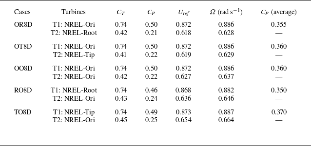
for different cases are presented in table 1.
The performance of five different tandem configurations simulated in the present study. For all cases, the TSR is maintained at 8.0 for both turbines. OR8D: NREL-Ori
 $\rightarrow$
NREL-Root. OT8D: NREL-Ori
 $\rightarrow$
NREL-Tip. OO8D: NREL-Ori
 $\rightarrow$
NREL-Ori. RO8D: NREL-Root
 $\rightarrow$
NREL-Ori. TO8D: NREL-Tip
 $\rightarrow$
NREL-Ori.

Table 1. Long description
The table presents the performance metrics of five different tandem configurations of turbines. It includes seven columns: Cases, Turbines, C_T, C_P, U_ref, Ω (rad s^-1), and C_P (average). The table has five rows, each representing a different configuration: OR8D, OT8D, OO8D, RO8D, and TO8D. Each row lists the turbines involved, their thrust coefficient (C_T), power coefficient (C_P), reference velocity (U_ref), rotational speed (Ω), and the average power coefficient (C_P average). Row 1: OR8D, T1: NREL-Ori, T2: NREL-Root, C_T values 0.74 and 0.42, C_P values 0.50 and 0.21, U_ref values 0.872 and 0.618, Ω values 0.886 and 0.628, C_P average 0.355. Row 2: OT8D, T1: NREL-Ori, T2: NREL-Tip, C_T values 0.74 and 0.41, C_P values 0.50 and 0.22, U_ref values 0.872 and 0.619, Ω values 0.886 and 0.629, C_P average 0.360. Row 3: OO8D, T1: NREL-Ori, T2: NREL-Ori, C_T values 0.74 and 0.42, C_P values 0.50 and 0.22, U_ref values 0.872 and 0.627, Ω values 0.886 and 0.637, C_P average 0.360. Row 4: RO8D, T1: NREL-Root, T2: NREL-Ori, C_T values 0.74 and 0.43, C_P values 0.46 and 0.24, U_ref values 0.868 and 0.636, Ω values 0.882 and 0.646, C_P average 0.350. Row 5: TO8D, T1: NREL-Tip, T2: NREL-Ori, C_T values 0.74 and 0.45, C_P values 0.49 and 0.25, U_ref values 0.873 and 0.654, Ω values 0.887 and 0.664, C_P average 0.370.
The computational domain. Turbines T1 and T2 represent the upstream and downstream turbines, respectively. The precursory ABL turbulent inflow is introduced at the inlet boundary, as indicated by the blue lines. Turbine T1 is positioned at a distance
 $3.5D$
from the inlet, with inter-turbine spacing
 $S_x = 8D$
used in the simulations. Turbine T2 is located
 $11.5D$
from the outlet. Both turbines are placed at the centre of the spanwise direction, maintaining an aligned configuration. The vertical length is set to 1 km, representing the thickness of the ABL.

The computational domain (shown in figure 1) is configured to ensure that the streamwise length is sufficiently large to encompass the turbine downstream locations of interest, the impact of the spanwise boundary on wake meandering is negligible, and the height (
 $L_z=1$
km) is typical for the thickness of the ABL. As seen, the upstream turbine is located at
 $3.5D$
from the inlet and in the middle of the spanwise direction, with its hub located at
 $z_{hub}$
from the ground (
 $z$
direction). According to previous studies (Medici et al. Reference Medici, Ivanell, Dahlberg and Alfredsson2011; Meyer Forsting Reference Meyer Forsting2017; Li et al. Reference Li, Dong and Yang2022; Dong et al. Reference Dong, Qin, Li and Yang2023), placing the turbine
 $3.5D$
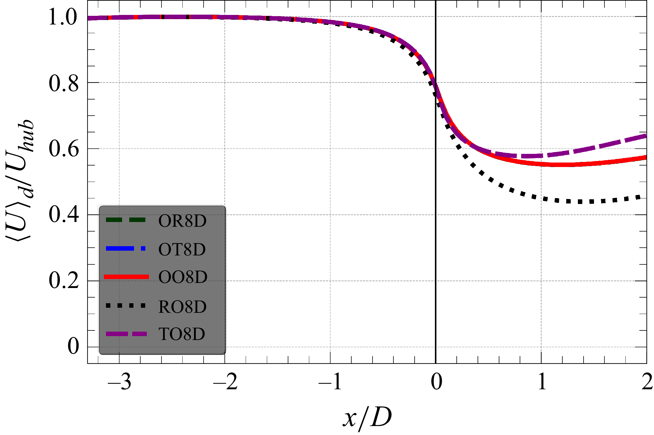
from the inlet is sufficient to ensure an undisturbed induction zone. To illustrate this, the time- and disk-averaged streamwise velocity is calculated and shown in figure 2. As seen, the induction effects vanish approximately
 $2D$
upstream of the first turbine for all the considered cases.
The downstream turbine is located
 $8D$
from the upstream one with aligned configuration. The computational domain, depicted in figure 1, has dimensions
 $L_x \times L_y \times L_z = 23D \times 7D \times 7.9D$
discretised using a Cartesian grid with
 $N_x \times N_y \times N_z = 461 \times 281 \times 231$
in the streamwise, spanwise and vertical directions, respectively. A uniform mesh is employed with grid spacings
 $\Delta x = D / 20$
and
 $\Delta y = D / 40$
in the
 $x$
and
 $y$
directions, respectively. In the vertical direction, the grid spacing is
 $\Delta z = D/40$
in the
 $[0, 2D]$
region, and gradually stretched to the top boundary. For all cases, the time step is set to
 $\Delta t = 0.0014D/U_{\textit{hub}}$
. The grid used in the present work is akin to our previous work, where the grid refinement study had been carried out (Dong et al. Reference Dong, Qin, Li and Yang2023). After the flow is fully developed within the computational domain, simulations run for another more than
 $1500$
rotor revolutions for sufficient time-averaged analysis and to capture the low-frequency modes of the wake meandering induced by the large eddies from the ABL flow.
Time- and disk-averaged streamwise velocity upstream of the turbine. Note that the OO8D, OT8D and OR8D curves overlap in the induction zone, as the upstream turbine is the same in these three cases.

The simulated tandem-turbine cases are designated by their upstream–downstream blade combinations: (i) OO8D for NREL-Ori
 $\rightarrow$
NREL-Ori; (ii) OR8D for NREL-Ori
 $\rightarrow$
NREL-Root; (iii) OT8D for NREL-Ori
 $\rightarrow$
NREL-Tip; (iv) RO8D for NREL-Root
 $\rightarrow$
NREL-Ori; (v) TO8D for NREL-Tip
 $\rightarrow$
NREL-Ori. Additionally, a no-turbine case (NoT), employing the same computational set-up, is also conducted as a reference for analyses. The upstream and downstream turbines are denoted as T1 and T2, respectively;
 $S_x = 8D$
is the distance between T1 and T2. For clarity, the simulated cases are divided into two categories. Scenario I (OO8D, OR8D and OT8D) represents the wake inflow cases, where the upstream turbine remains the same, and different blade designs are used for the downstream turbine. The discussion in these cases focuses on revealing the wake dynamics for different blade designs under wake inflows. Scenario II (OO8D, RO8D and TO8D) emphasises the effect of blade design on the performance and wake dynamics of the downstream turbine. The paper focuses on the wake of T2 unless otherwise specified. Within these two scenarios, the turbine with a different blade design acts as either a wake receiver (scenario I) or a wake generator (scenario II), with the other turbine fixed as the original design. Homogeneous configurations such as RR8D and TT8D, which are of practical interest but beyond the designed scenarios, are not considered in this study.
The precursory LES simulation with ground roughness length
 $z_0 =0.001$
m is conducted and saved to generate ABL turbulent inflows. The simulations are pressure-driven, and thermal stability is not modelled. The disk-averaged wind speed (
 $U/U_{\textit{hub}}$
) and turbulence intensity (
 $TI$
) are 0.889 % and 5.43 % at the position of T1, and 0.884 % and 5.98 % at the position of T2, respectively. Further details about the inflow simulations can be found in our previous studies (Dong Reference Dong, Li, Qin and Yang2022a
, et al. Reference Dong, Qin, Li and Yang2023). At the outlet, the Neumann boundary condition is applied. At the top and spanwise boundaries, the free-slip boundary condition is employed. On the ground, a wall model is utilised, and the wall shear stress is computed using the logarithmic law for rough walls with roughness length
 $z_0 = 0.001$
m.
3. Results
3.1. Time-averaged statistics
3.1.1. Power outputs
The axial force coefficients (
 $C_{\!F_a}=F_a/(\rho \pi R U_{\textit{hub}}^2)$
) of both T1 and T2 are shown in figure 3, where
 $F_a$
is the axial component of the force per unit length along the blade span. As shown in figure 3(a), the force distributions of T1 are similar to our previous single turbine results (Dong et al. Reference Dong, Qin, Li and Yang2023). The loads on T2 (figure 3
b) are generally lower and modified due to the waked inflow generated by T1. For T2, special attention is paid to the scenario I cases to examine the load distributions of different blade designs under waked inflow. Relatively lower axial loads are observed along the blade radial direction for the OT8D case, which are significantly different from those observed under freestream inflows. For the comparisons among OO8D, RO8D and TO8D cases (scenario II), the overall distributions of loads are approximately the same except near the blade tip region, where relatively lower and higher loads are observed in the TO8D and RO8D cases, respectively, indicating the influence of upstream turbine wakes on the loading on the downstream unit. For the NREL-Tip blade, the loading is shifted towards the outer blade region from an aerodynamic design perspective. The resulting non-monotonic distribution should therefore not be interpreted as a structurally or aeroelastically optimised blade design, since structural stability was not considered in the present study.
Rotor-scale-normalised axial force coefficient distributions along the blade span for both (a) the upstream turbine T1 and (b) the downstream turbine T2.

Figure 3. Long description
Two line graphs depict rotor-scale-normalised axial force coefficient distributions along the blade span for upstream and downstream turbines. Panel A: The line graph shows the axial force coefficient distributions for the upstream turbine T1. The x-axis represents the normalized radial position along the blade span (r/R), ranging from 0 to 1. The y-axis represents the axial force coefficient (C_Fa), ranging from 0 to 0.8. The graph includes five data series: OR8D (green solid line), OT8D (blue dashed line), OO8D (red dotted line), RO8D (black dashed-dotted line), and TO8D (magenta dashed line with triangles). The data series show varying trends, with peaks and troughs at different radial positions. Panel B: The line graph shows the axial force coefficient distributions for the downstream turbine T2. The x-axis represents the normalized radial position along the blade span (r/R), ranging from 0 to 1. The y-axis represents the axial force coefficient (C_Fa), ranging from 0 to 0.8. The graph includes the same five data series as Panel A, with similar trends and variations in the axial force coefficient distributions.
The obtained thrust coefficients (
 $C_T$
) and power coefficients (
 $C_{\!P}$
) are shown in table 1, and the corresponding equations are
 \begin{align} C_{\!P} = \frac {{\varOmega } M}{0.5 \rho A {U_{\textit{ref}}^3}}, \\[-12pt]\nonumber \end{align}
 \begin{align} C_T= \frac {\textit{Fn}}{0.5 \rho A {U_{\textit{ref}}^2}}, \end{align}
where
 $\varOmega$
is the rotational velocity,
 $M$
is the torque, and
 $A$
is the rotor swept area of the turbine. Interesting results can be obtained in scenario II. As observed, placing the root-loaded or tip-loaded turbine upstream (i.e. RO8D or TO8D) allows the downstream turbine to generate more power. Among these, the TO8D configuration yields the highest average power output, with an improvement of approximately
 $3\,\%$
. To assess the sensitivity of this gain to wind direction, we investigated cases in which the two turbines are not perfectly aligned with the mean wind direction, but instead experience a wind direction uniformly distributed within
 $\pm 5^\circ$
of the line connecting the turbines. Under these conditions, the power gain of the TO8D configuration decreases from 3 % to approximately 2 %. This suggests that while non-aligned conditions reduce the benefit of enhanced wake recovery, the specific blade design still offers a performance advantage under typical operational variations. However, this advantage indeed depends on the climatology of the site. The evaluation of these effects at a wind farm scale will be the subject of future work.
3.1.2. Mean wake flow
In this subsubsection, the time-averaged field is analysed to show the overall wake dynamics for different tandem configurations, categorised into two categories: scenario I (OR8D, OT8D and OO8D), and scenario II (RO8D, TO8D and OO8D). We focus on the analysis of the wake dynamics of T2 unless stated otherwise. Figure 4 presents contours of streamwise velocity and turbulent kinetic energy (TKE) on the vertical-streamwise section. Overall, it is observed from scenario I cases that blade designs are still capable of affecting wake dynamics under wake inflows. For scenario II cases, some impacts of upstream blade design on downstream wakes are also observed, especially the faster wake recovery of T2 observed in the RO8D case.
Time-averaged normalised streamwise velocity (a) and TKE (b) contours for (a) OR8D, (b) OT8D, (c) OO8D, (d) RO8D and (e) TO8D cases on the
 $x{-}z$
vertical plane passing through the rotor centre (
 $y=0$
).

Quantitative results for the vertical profiles of the normalised streamwise velocity deficit (
 $\Delta U / U_{\textit{hub}}$
) and turbine-added TKE (
 $\Delta k / U_{\textit{hub}}^2$
) are shown in figure 5. The definitions of
 $\Delta U$
and
 $\Delta k$
are
 \begin{align} \Delta U = U_{\textit{NT}} - U, \\[-12pt]\nonumber \end{align}
 \begin{align} \Delta k = k -k_{\textit{NT}}, \end{align}
where the subscript
 $_{\textit{NT}}$
denotes the quantities obtained in the simulation without a wind turbine.
Under waked inflow conditions, wake evolution of the downstream unit (T2 in scenario I cases) shows that the root-loaded design (NREL-Root) creates a larger velocity deficit and higher turbine-added TKE in the near wake than the baseline, and exhibits a faster overall recovery rate. Conversely, the tip-loaded design (NREL-Tip) generates a smaller deficit and less turbine-added TKE in the near wake, but recovers at a slower rate. In scenario II, the upstream root-loaded design increases inflow turbulence intensity for the downstream turbine in the RO8D case, which exhibits higher turbine-added TKE in the lower-half wake at
 $x/D=1, 2, 3$
, and a consequently faster wake recovery compared to the OO8D and TO8D cases.
Time-averaged vertical profiles of (a) the streamwise velocity deficit and (b) turbine-added TKE, downstream of T2. The black horizontal dashed lines indicate the positions of blade bottom tip and top tip, respectively.

Figure 5. Long description
The image contains two sets of line graphs showing time-averaged vertical profiles of streamwise velocity deficit and turbine-added TKE downstream of turbine T2. Each set includes multiple line graphs representing different blade designs. Panel A: The first set of graphs shows the streamwise velocity deficit (ΔU/U_hub) at various downstream distances (x - x_T2) from 1D to 10D. The vertical axis represents the normalized height (z/D), and the horizontal axis represents the normalized velocity deficit (ΔU/U_hub). The black horizontal dashed lines indicate the positions of the blade bottom tip and top tip. Different line styles and colors represent various blade designs: OR8D (green dashed), OT8D (blue dashed), OO8D (red solid), RO8D (black dotted), and TO8D (purple solid). Panel B: The second set of graphs shows the turbine-added turbulent kinetic energy (TKE) (Δk/U_hub^2) at the same downstream distances. The vertical axis represents the normalized height (z/D), and the horizontal axis represents the normalized TKE (Δk/U_hub^2). The same blade designs are represented by the same line styles and colors as in Panel A. The graphs illustrate how different blade designs affect the velocity deficit and TKE downstream of the turbine, highlighting the impact of blade design on wake dynamics.
The streamwise evolutions of the time- and disk-averaged streamwise velocity (
 $\langle U \rangle _d / U_{\textit{hub}}$
) and TKE (
 $\langle k \rangle _d / U_{\textit{hub}}^2$
) are shown in figures 6(a) and 6(b), respectively. The wakes from different blade designs under waked inflows (scenario I) are found to vary similarly to those under freestream inflow for both streamwise velocity and TKE. Specifically, the amplitude of streamwise velocity is lower in the near wake when the aerodynamic load near the root is higher, but becomes approximately the same in the far wake for all the scenario I cases (OO8D, OR8D, OT8D). Comparing T2 in OR8D and with OT8D, the TKE is observed being higher and located at further turbine downstream locations. For scenario II cases (OO8D, RO8D, TO8D), higher TKE of the inflow for the T2 wind turbine is clearly demonstrated for the T1 wind turbine with higher aerodynamic loads near the root, which then causes a higher recovery rate for the downstream wind turbine’s wake. Remember that the turbine-added TKE values of T2’s wake for the scenario II cases are approximately the same (figure 5), indicating that the differences in TKE shown in this figure are mainly from T2’s inflow. Further, figures 6(c) and 6(d) present the evolutions of the time- and disk-averaged streamwise velocity and TKE normalised by their respective values
 $1D$
upstream of T2. Similar trends in streamwise velocity are observed when comparing figure 6(c) to figure 6(a). However, the TKE levels for the TO8D and RO8D cases in scenario II are significantly higher and lower, respectively, due to the wake of T1. These normalised results demonstrate that the root-loaded design continues to exhibit higher relative turbulence production and faster wake recovery.
Time- and disk-averaged (a) streamwise velocity
 $\langle U \rangle _d / U_{\textit{hub}}$
and (b) TKE
 $\langle k \rangle _d / U_{\textit{hub}}^2$
normalised by
 $U_{\textit{hub}}$
, (c) streamwise velocity
 $\langle U \rangle _d / U_{\textit{T}2(-1\textit{D})}$
and (d) TKE
 $\langle k \rangle _d / k_{\textit{T}2(-1\textit{D})}$
normalised by the value at
 $1D$
upstream of T2, along the downstream direction. The vertical black lines at
 $x-x_{{T2}}/D=8$
indicate the presence of T2.

Then the mean kinetic energy (MKE) budget equation, shown in (3.5), is analysed to further reveal the detailed mechanism for wake recovery.
 \begin{align} \begin{aligned} 0 & = -\langle u_{\!j} \rangle \frac {\partial \langle u_i \rangle \langle u_i \rangle /2}{\partial x_{\!j}} - \frac {\partial }{\partial x_{\!j}} \left ( \frac {1}{\rho } \langle p \rangle \langle u_{\!j} \rangle + \langle u_i^{^\prime } u_{\!j}^{^\prime } \rangle \langle u_i \rangle - 2(\nu +\nu _t)S_{ij}\langle u_i \rangle \right ) \\[3pt] &+ \langle u_i^{^\prime } u_{\!j}^{^\prime } \rangle \frac {\partial \langle u_i \rangle }{\partial x_{\!j}} - 2(\nu +\nu _t)S_{ij}\frac {\partial \langle u_i \rangle }{\partial x_{\!j}} \end{aligned} \end{align}
To simplify the analysis of the wake as a whole, (3.5) is integrated over a square control surface with the spanwise and vertical directions, ranging from
 $y_1=y_c-R$
to
 $y_2=y_c+R$
, and
 $z_1 =z_{\textit{hub}}-R$
to
 $z_2=z_{\textit{hub}}+R$
, along different
 $x$
positions. The integral form of the MKE equation takes the form
 \begin{align} 0 = \textit{MC} + \textit{PT} + \textit{TC} + \textit{DF} + \textit{TP} + \textit{DP}, \end{align}
where
 $\textit{MC}$
,
 $\textit{PT}$
,
 $\textit{TC}$
,
 $\textit{DF}$
,
 $\textit{TP}$
and
 $\textit{DP}$
represent the mean convection term, the pressure transport term, the turbulent convection term, the diffusion term, the turbulence production term and the dissipation term, respectively. The detailed mathematical definitions of these six terms can be found in Dong et al. (Reference Dong, Qin, Li and Yang2023).
The MKE budget analysis for wakes of T2 for (a) OR8D, (b) OT8D, (c) OO8D, (d) RO8D and (e) TO8D cases. All terms are normalised using
 $U_{\textit{hub}}$
and
 $D$
.

Figure 7. Long description
Five line graphs depict the MKE budget analysis for wakes of T2 for different cases. Panel A: The line graph for the OR8D case shows the normalized terms on the vertical axis against the normalized distance on the horizontal axis. The red solid line represents MC, the green dashed line represents PT, the blue dashed-dotted line represents TC, the black dashed line represents TP, the purple dotted line represents DF, and the yellow dotted line represents DP. Panel B: The line graph for the OT8D case follows the same format as Panel A. Panel C: The line graph for the OO8D case follows the same format as Panel A. Panel D: The line graph for the RO8D case follows the same format as Panel A. Panel E: The line graph for the TO8D case follows the same format as Panel A. Each graph shows the trends of different terms in the MKE budget analysis, with varying patterns and interactions among the lines.
The evolution of (a)
 $\textit{TC}$
and (b)
 $\textit{TP}$
terms downstream of T2.

Figure 8. Long description
Two line graphs depict the evolution of terms downstream of T2. Panel A: The line graph shows the evolution of the TP term. The horizontal axis is labeled (x - xT2)/D and ranges from 0 to 10. The vertical axis ranges from -0.005 to 0.001. The graph includes five different lines representing OR8D, OT8D, OO8D, RO8D, and TO8D, each with distinct colors and line styles. The lines show various trends, with some increasing, decreasing, or fluctuating as they move from left to right. Panel B: The line graph shows the evolution of the TC term. The horizontal axis is labeled (x - xT2)/D and ranges from 0 to 10. The vertical axis ranges from 0.003 to 0.011. Similar to Panel A, this graph includes five different lines representing OR8D, OT8D, OO8D, RO8D, and TO8D, each with distinct colors and line styles. The lines exhibit different patterns, with some peaking and then declining as they move from left to right.
Figure 7 presents the streamwise evolution of six terms under five distinct tandem configurations, with the comparisons of the
 $\textit{TP}$
and
 $\textit{TC}$
terms particularly examined in figure 8. The
 $\textit{TP}$
term is always negative in the MKE budget, and represents the extraction of MKE due to turbulence generation. In contrast, the
 $\textit{TC}$
term is positive and reflects the spatial transport of MKE due to turbulence, and is directly related to the momentum entrainment through the Reynolds stress. First, the effects of blade designs on MKE budgets under waked inflows are similar to freestream inflows. Three key points include: (i) the tip-loaded design induces a larger drop on the
 $\textit{PT}$
term compared with the root-loaded design; (ii) the root-loaded design has a somewhat overall longer streamwise range with intense
 $\textit{TP}$
and
 $\textit{TC}$
terms; (iii) the peaks of the
 $\textit{TP}$
term of the tip-loaded design occur as locations closer to the turbine when compared with the root-loaded design. For the scenario II cases, the higher inflow turbulence intensity for blade designs with higher aerodynamic load near the root is found consistently increasing the amplitudes of the
 $\textit{TC}$
term, thus promoting the velocity recovery and turbulence generation.
3.2. Wake meandering
In this subsection, the wake meandering characteristics are analysed for the considered tandem configurations. Before carrying out detailed analysis, the wake structures are presented in figure 9, where the iso-surfaces are constructed using the streamwise velocity, with the corresponding contours displayed on the background slices.
Instantaneous wakes for different tandem configurations: (a) OR8D, (b) OT8D, (c) OO8D, (d) RO8D and (e) TO8D. The iso-surfaces represent the normalised streamwise velocity.

3.2.1. Meandering characteristics
The spatial distribution of TKE is highly correlated with wake meandering. In the near-wake region, TKE is primarily generated by vortices within the tip shear layers. As these shear layers merge downstream, they define the end of the near wake, and mark the onset of wake meandering, which then becomes one key mechanism influencing the TKE generation and distribution. Figure 10 illustrates the streamwise evolution of TKE in the near-wake of downstream turbine T2. Defining the merging point of the tip shear layers at the wake centre is threshold-dependent. In this work, the merger is quantified by the radial growth rate of the high-TKE regions associated with the tip shear layer. For scenario I cases, the radial growth rate is generally higher for the root-loaded blade design than for the other two designs. This suggests an earlier onset of wake meandering for the root-loaded design when compared with other two designs under waked inflow conditions, a trend that is consistent with its behaviour in freestream inflows. For scenario II, the results demonstrate that the upstream blade design directly influences the extent of the high-TKE region from the wake’s inception, thereby amplifying downstream wake meandering, highlighting its potential as a wind farm control parameter.
TKE contours on the
 $y{-}z$
plane at various downstream positions for turbine T2 in cases (a) OR8D, (b) OT8D, (c) OO8D, (d) RO8D and (e) TO8D.

Figure 10. Long description
A heat map representing turbulence kinetic energy contours on the plane at various downstream positions for turbine T2 in cases OR8D, OT8D, OO8D, RO8D, and TO8D. The heat map is organized in a grid layout with five columns and six rows, each representing a different downstream position. The axes are labeled with z/D on the vertical axis and y/D on the horizontal axis, where D is the diameter of the turbine. The color scale ranges from blue to red, indicating increasing values of turbulence kinetic energy, with blue representing lower values and red representing higher values. The range of values shown is from 0 to 0.026 k/U_hub^2. Each column corresponds to a different blade design case: OR8D, OT8D, OO8D, RO8D, and TO8D. Each row represents a different downstream position, labeled as 0D, 0.5D, 1D, 1.5D, 2D, and 3D. The heat maps show the distribution of turbulence kinetic energy at these positions, with higher values concentrated in the central regions and lower values towards the edges. The patterns indicate how different blade designs affect the wake dynamics and velocity recovery downstream of the turbine.
Double-Gaussian and single-Gaussian fits of the near and far wakes of the downstream turbine T2 with the original velocity contours embedded in the background for cases (a) OR8D, (b) OT8D, (c) OO8D, (d) RO8D and (e) TO8D. The blue dashed lines indicate the transition position from double-Gaussian to single-Gaussian. All data are extracted at the hub height horizontal planes.

While the near wake is approximated using a double-Gaussian function (Keane et al. Reference Keane, Aguirre, Ferchland, Clive and Gallacher2016; Schreiber et al. Reference Schreiber, Balbaa and Bottasso2020), the far wake is well represented by a single-Gaussian function (Bastankhah & Porté-Agel Reference Bastankhah and Porté-Agel2014). Consequently, the transition position from the near wake to the far wake is defined as the most upstream position where the single-Gaussian fit properly describes the velocity deficit profile. The corresponding fitting functions are given as
 \begin{align} &\quad \Delta U(x,y) = \Delta U_c(x) \exp\left ( \frac {-(y-y_c(x))^2}{2\sigma (x)^2}\right )\!, \\[-12pt]\nonumber \end{align}
 \begin{align} \Delta U(x,y) =& \Delta U_{c_d}(x) \left ( \exp \left ( \frac {-(y - y_{c_d}(x))^2}{2\sigma _d^2(x)} \right ) + \exp \left ( \frac {-(y + y_{c_d}(x))^2}{2\sigma _d^2(x)} \right ) \right )\!, \end{align}
where
 $\Delta U(x,y)$
is the velocity deficit distribution,
 $\Delta U_c(x)$
is the velocity deficit at the wake centre,
 $y_c(x)$
is the spanwise position of the fitted wake centre, and
 $\sigma (x)$
is the standard deviation of the single-Gaussian distribution. Similarly,
 $\Delta U_{c_d}(x)$
is the velocity deficit at the double-Gaussian wake centre,
 $y_{c_d}(x)$
is the spanwise position of the fitted wake centre of the double-Gaussian distribution, and
 $\sigma _d(x)$
is the standard deviation of the double-Gaussian distribution.
The fitting results of T2’s wake are shown in figure 11. We assume that the streamwise position for the transition from the near wake to the far wake is the position where the error for single-Gaussian fit is lower than for double-Gaussian fit. The blue dashed line indicates the first position where the double-Gaussian transitions into the single-Gaussian distribution. Data in figure 11 are extracted at the hub height horizontal planes. As depicted in this figure, the transition is postponed for turbine T2 in the OT8D and TO8D cases in comparison with other cases. In contrast, the OR8D and RO8D cases exhibit an earlier transition. This trend provides quantitative insight into the onset of wake meandering, which is discussed later (see figure 18).
To investigate the statistics of wake meandering, the instantaneous velocity deficit profiles in the far-wake region are fitted using a single-Gaussian function to identify the transverse positions of instantaneous wake centres. To reduce small-scale fluctuations in the instantaneous wake field, a spatial box filtering with width
 $1D$
is conducted prior to the Gaussian fitting. The typical results at an instant are displayed in figure 12, with the left-hand column for the instantaneous wake field, and the middle and right-hand columns for the velocity deficit profiles of turbines T1 and T2.
Instantaneous velocity deficit contours for tandem configurations with the corresponding original (black), filtered (blue) and fitted (red) velocity deficit profiles. The left-hand column shows the original velocity deficit contours (ai), with the black dashed lines indicating the fitted wake centres along different downstreams. The middle and right-hand columns show the original, filtered and fitted wakes of (aii) T1 at
 $x=5D$
, and (aiii) T2 at
 $x=15D$
.

Standard deviations of the wake centres at various T2 downstream positions.

Temporal variations of the instantaneous spanwise wake centre positions of cases (a) OR8D, (b) OT8D, (c) OO8D, (d) RO8D and (e) TO8D at
 $19D$
downstream for
 $y_c$
of all resolved frequencies (the left-hand column),
 $y_{c_1}$
of the low-frequency part with
 $\textit{St} \lt 0.1$
(the middle column), and
 $y_{c_2}$
of the high-frequency part with
 $\textit{St} \gt 0.1$
(the right-hand column). The time
 $t$
is normalised by using
 $D$
and
 $U_{\textit{hub}}$
, i.e.
 $T = D/U_{\textit{hub}}$
.

Figure 14. Long description
The image contains multiple line graphs depicting temporal variations of the instantaneous spanwise wake center positions for different cases at various downstream positions. The graphs are organized into five rows labeled (a) OR8D, (b) OT8D, (c) OO8D, (d) RO8D, and (e) TO8D. Each row contains three columns of line graphs. Panel A: The left-hand column shows the variations for all resolved frequencies. The middle column shows the low-frequency part with a specific frequency range, and the right-hand column shows the high-frequency part with another specific frequency range. The x-axis represents the normalized time using a specific formula, and the y-axis represents the spanwise wake center positions normalized by a specific diameter. Each graph contains a red line representing the data and a blue circle highlighting specific points of interest. The graphs illustrate how the spanwise wake center positions vary over time for different cases and frequency ranges.
The obtained standard deviations of the instantaneous wake centre positions (i.e. the amplitudes of wake meandering) are plotted in figure 13. Results from the scenario I cases (OO8D, OR8D, OT8D) show that under waked inflows, the root-loaded blade design induces wake meandering with higher amplitudes in the far-wake region compared to the other two designs – a trend consistent with behaviour observed under freestream inflows. Among the scenario II cases (OO8D, RO8D, TO8D), the meandering amplitude is the greatest when the root-loaded design is placed upstream, and the smallest when the tip-loaded design is placed upstream. It is also notable that in the RO8D configuration, the meandering amplitude of T2 begins to exceed that of the other two configurations at a location close to T2 (
 $\approx 2D$
), which is significantly earlier than the corresponding onset in the OR8D configuration under scenario I. This interesting result highlights the potential of using blade designs to control wake dynamics over an extensive streamwise range. We will investigate the underlying mechanism in the remainder of the paper.
The correlations of instantaneous wake centre positions between the OO8D configuration and other configurations are examined. To analyse correlations across different scales, the time series of transverse wake centre positions are decomposed into large-scale (
 $\textit{St} \lt 0.1$
) and small-scale (
 $\textit{St} \gt 0.1$
) components using a fast Fourier transform. The overall wake centre is denoted by
 $y_c$
, while its large- and small-scale components are denoted by
 $y_{c_1}$
and
 $y_{c_2}$
, respectively. The temporal variations of both parts are presented in figure 14. The large-scale component is primarily influenced by incoming large eddies, whereas the small-scale fluctuations are largely governed by the wake shear layer itself. A higher degree of similarity is observed in the large-scale motions. The correlations for both scales are quantified and plotted in figure 15. Results show that
 $y_{c_1}$
maintains a strong correlation (
 $R_{y_c} \gt 0.9$
), while the correlation of
 $y_{c_2}$
is significantly weakened, especially for the RO8D case. This indicates the dominant effect of wake shear layer instability on wake meandering for the RO8D configuration. The fact that the correlation in the OR8D case falls below that of the OT8D case in T2’s wake further implies greater shear layer instability in the root-loaded design. Moreover, the comparison between RO8D and OR8D cases indicates that a root-loaded turbine exerts a stronger impact on overall wake dynamics when positioned upstream. An interesting observation is that the correlation of the TO8D case with OO8D decreases in T1’s wake but increases in T2’s wake.
Correlation coefficients between tandem configurations and the OO8D configuration for wake of T2 of (a) all resolved frequencies
 $y_c$
, (b) low-frequency part
 $y_{c_1}$
, and (c) high-frequency part
 $y_{c_2}$
.

The PSD
 ${S(v')}/({D U_{\textit{hub}}})$
of the instantaneous spanwise velocity fluctuations for the inflows of (a) T1 (
 $x=-3D$
) and (b) T2 (
 $x-x_{T2}= -1D$
) along the wake centreline position (
 $y=0R$
).

3.2.2. Meandering mechanism
This subsubsection investigates the mechanism through which blade design influences wake meandering in tandem wind turbine configurations. The factors governing wake dynamics are broadly categorised as those originating from ambient turbulence and those inherent to the turbine itself. Accordingly, the inflows for both the upstream (T1) and downstream (T2) turbines are first examined. The analysis then delves into the role of blade design in mediating both ambient–turbine and turbine–turbine interactions.
The power spectral density (PSD) of the inflow velocity fluctuations is presented in figure 16. Figure 16(a) displays the characteristics of the freestream inflow. As observed, the TKE is distributed across a broad range of scales, with Strouhal numbers (
 $\textit{St}$
) ranging from 0.01 to 10. Distinct spectral peaks are evident at several values, such as
 $\textit{St} \approx 0.03$
and
 $0.2$
. Here, the Strouhal number is defined as
 $\textit{St} = fD / U_{\textit{hub}}$
, where
 $f$
denotes frequency,
 $D$
is the rotor diameter, and
 $U_{\textit{hub}}$
is the streamwise inflow velocity at hub height.
For the inflow of T2, which incorporates both the wake from T1 and the ambient turbulence, the ambient large-scale structures (with
 $\textit{St} \approx 0.03$
) persist in both scenario I and scenario II, and exhibit some degree of amplitude amplification, which was also observed in our previous study (Yang & Sotiropoulos Reference Yang and Sotiropoulos2019b
). More notably, coherent motions within the range
 $\textit{St} = 0.1$
–
 $0.4$
become dominant over the ambient large-scale structures. The elevated energy content in this frequency range is attributed to the wake shear layer instability generated by T1.
The pre-multiplied PSDs (FPSD) of
 $v'$
, focusing on scales associated with wake shear layers, are further examined in figure 17 to illustrate the downstream evolution of coherent motions. These scales can be categorised into two ranges:
 $0.1 \lt St \lt 1$
, corresponding to meandering motion, and
 $\textit{St} \gt 1$
, associated with small-scale motions originating from the tip shear layer. At a location
 $1D$
downstream of the turbine, the
 $\textit{St} \gt 1$
components dominate. The tip-loaded design demonstrates a stronger ability to generate small-scale fluctuations in both freestream and waked inflows. In contrast, the root-loaded design produces meandering motions with higher amplitude, which also emerge at earlier downstream positions under both inflow conditions.
In scenario II, which investigates how wakes from different blade designs influence downstream wakes, the high-amplitude wake meandering generated by the root-loaded design is observed to directly affect the meandering of the downstream wake. This effect starts being dominant even at
 $1D$
downstream of T2. An interesting observation is that by
 $10D$
downstream of T2, the pre-multiplied PSD distributions become similar in shape across different cases, despite variations in peak amplitudes – a notable contrast to the significant differences seen at upstream locations and in the wakes of T1. This suggests an asymptotic behaviour in the coherent structures deep within the wind farm.
Pre-multiplied spectra of
 $v^\prime$
at rotor centreline (
 $y=0R$
) along downstream positions of (a) T1 and (b) T2.

Figure 17. Long description
The image contains multiple line graphs depicting pre-multiplied power spectral densities (PSDs) at different downstream positions. The graphs are organized into two columns, each representing different turbine positions (T1 and T2). Each column contains three line graphs, each corresponding to a specific downstream position (x = 1D, 4D, 7D for T1 and x = 9D, 12D, 18D for T2). The horizontal axis of each graph represents the Strouhal number (St) on a logarithmic scale, while the vertical axis represents the pre-multiplied PSDs normalized by the hub velocity squared (fΦ(v)/U_hub^2). The legend at the top identifies different data series with distinct colors and line styles: OR8D (green dashed), OT8D (blue dash-dot), OO8D (red solid), RO8D (black dotted), and TO8D (purple dash-dot). Panel A: The left column shows graphs for turbine position T1 at downstream positions x = 1D, 4D, and 7D. Each graph displays multiple lines representing different data series, with varying peaks and trends across the Strouhal number range. Panel B: The right column shows graphs for turbine position T2 at downstream positions x = 9D, 12D, and 18D. Similar to Panel A, each graph displays multiple lines with distinct peaks and trends. The graphs illustrate how the pre-multiplied PSDs vary with downstream position and different data series, highlighting the scales associated with wake shear layers.
To quantify the onset position of wake meandering downstream of T2, figure 18 presents the pre-multiplied PSD at different
 $x-x_{{T2}}$
. The peak highlighted by the vertical yellow line indicates the signal of the onset of wake meandering. Wake meandering occurs earlier for the root-loaded cases (at approximately
 $1D$
and
 $0.75D$
for OR8D and RO8D, respectively), followed by the OO8D case (at approximately
 $2.25D$
), and later for the tip-loaded cases (at approximately
 $3D$
and
 $2.5D$
for OT8D and TO8D, respectively). This trend is consistent with the transition from the near wake to the far wake discussed in figure 11.
Pre-multiplied spectra of
 $v^\prime$
at rotor centreline (
 $y=0R$
) for different tandem configurations downstream of T2, illustrating the streamwise position of the onset of wake meandering.

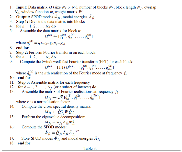
The SPOD is conducted to understand the underlying flow mechanism. The transverse velocity fluctuations (
 $v^\prime$
) in the horizontal hub-height plane are employed for the SPOD analysis with
 $N_f = 1024$
snapshots per window and
 $N_b = 18$
blocks. A standard Hann window is applied to reduce spectral leakage. The eigenvalue spectrum as a function of frequency is shown in figure 19, with the first and second eigenvalue spectra plotted in red and blue, respectively. For the other modes, the shading of the curves gradually changes from black to white as the mode number increases from 3 to
 $N_b$
. As seen, the eigenvalues at various scales increase with comparison with the no-turbine case (NoT), indicating the amplification effect of wakes on the inflow turbulence. Among them, the meandering motion with
 $\textit{St} = 0.2$
–
 $0.4$
experiences the greatest amplification.
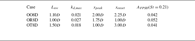
Key wake statistics of wind turbine T2 in scenario I:
 $L_{\textit{nw}}$
is near-wake length,
 $k_{\textit{d,max}}$
is peak disk-averaged TKE (
 $k_d/U_{\textit{hub}}^2$
),
 $x_{\textit{peak}}$
is location of peak TKE,
 $x_{\textit{onset}}$
is onset of wake meandering,
 $A_{\textit{FPSD}} (St=0.21)$
is FPSD amplitude at
 $\textit{St}=0.21$
(
 $x/D=18$
). Refer to figures 6, 11 and 17 for corresponding field or curve plots.

Table 2. Long description
The table presents key wake statistics of wind turbine T2 in scenario I. It includes five columns: Case, Lnw, kd,max, xpeak, xonset, and AFPSD(St = 0.21). The table has three rows, each representing a different case: OO8D, OR8D, and OT8D. Row 1: Case OO8D, Lnw 1.10D, kd,max 0.021, xpeak 2.00D, xonset 2.25D, AFPSD(St = 0.21) 0.042. Row 2: Case OR8D, Lnw 1.00D, kd,max 0.027, xpeak 1.75D, xonset 1.00D, AFPSD(St = 0.21) 0.052. Row 3: Case OT8D, Lnw 1.50D, kd,max 0.018, xpeak 1.00D, xonset 3.00D, AFPSD(St = 0.21) 0.041.
The SPOD eigenvalues as a function of frequencies for
 $v^\prime$
in the horizontal hub-height plane for (a) NoT, (b) OO8D, (c) OR8D, (d) OT8D, (e) RO8D, and (f) TO8D.

The first SPOD modes for low ambient flow frequencies (
 $\textit{St}=0.035$
,
 $0.07$
,
 $0.104$
) and wake meandering frequencies (
 $\textit{St}=0.21$
,
 $0.31$
,
 $0.42$
) are presented in figures 20 and 21, respectively. Two distinct mechanisms are identified: at low ambient flow frequencies, the shear layer instability primarily acts as a disturber, while at wake meandering frequencies, it acts as an amplifier. As shown in figure 20, the SPOD amplitudes (eigenvalues) change only marginally at
 $\textit{St}=0.035$
and
 $0.07$
, but increase significantly at
 $\textit{St}=0.104$
. The mode at
 $\textit{St}=0.104$
is unique, as it is clearly present in the ambient flow and is subsequently both disturbed and amplified by the wake. It is noted that at these low ambient flow frequencies, where integrated force is the dominant factor, the impact of blade design is negligible.
At wake meandering frequencies, a frequency-selection mechanism emerges, linking the strength of the design-induced near-wake shear layer to the overall wake evolution. The shear-layer instability influences the response to inflow disturbances, particularly at
 $\textit{St} \approx 0.21$
, where the downstream wake resonates with the upstream wake and strengthens the inflow structures. These structures evolve in the downstream direction, showing further intensification at the downstream turbine T2 (e.g. figure 21
a) before decaying at locations further downstream from T2 (e.g. figure 21
b). While these resonant behaviours are qualitatively consistent across all tandem configurations, the blade design significantly affects their onset and intensity. Specifically, the root-loaded design triggers an earlier onset and achieves higher peak intensities.
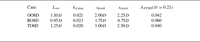
Key wake statistics of wind turbine T2 in scenario II:
 $L_{\textit{nw}}$
is near-wake length,
 $k_{\textit{d,max}}$
is peak disk-averaged TKE (
 $k_d/U_{\textit{hub}}^2$
),
 $x_{\textit{peak}}$
is location of peak TKE,
 $x_{\textit{onset}}$
is onset of wake meandering,
 $A_{\textit{FPSD}} (St=0.21)$
is FPSD amplitude at
 $\textit{St}=0.21$
(
 $x/D=18$
). Refer to figures 6, 11 and 17 for corresponding field or curve plots.

Table 3. Long description
The table presents key wake statistics of wind turbine T2 in scenario II. It includes five columns: Case, Lnw, kd,max, xpeak, xonset, and AFPSD(St = 0.21). The table has three rows labeled with different cases: OO8D, RO8D, and TO8D. Each row provides specific values for the columns. Row 1: Case OO8D, Lnw 1.10 D, kd,max 0.021, xpeak 2.00 D, xonset 2.25 D, AFPSD(St = 0.21) 0.042. Row 2: Case RO8D, Lnw 0.95 D, kd,max 0.023, xpeak 1.75 D, xonset 0.75 D, AFPSD(St = 0.21) 0.060. Row 3: Case TO8D, Lnw 1.25 D, kd,max 0.020, xpeak 3.00 D, xonset 2.50 D, AFPSD(St = 0.21) 0.040.
The SPOD modes of the spanwise velocity fluctuation for
 $\textit{St}$
values (a) 0.035, (b) 0.07 and (c) 0.104.

Figure 20. Long description
A set of heat maps representing spanwise velocity fluctuations for different values. The heat maps are organized into three rows labeled (a), (b), and (c), each corresponding to different values of 0.035, 0.07, and 0.104, respectively. Each row contains six panels, labeled (i) to (vi), representing different conditions or experiments. Panel A: The first row (a) includes panels (ai) to (avi) showing heat maps for the value 0.035. Each panel has axes labeled x/D and y/D, with x/D ranging from 0 to 18 and y/D ranging from -2.5 to 2.5. The color scale on the right indicates values from -0.005 to 0.005, with red representing higher values and blue representing lower values. Notable regions of high and low values are visible in each panel. Panel B: The second row (b) includes panels (bi) to (bvi) showing heat maps for the value 0.07. Similar to the first row, each panel has axes labeled x/D and y/D, with the same range. The color scale and notable regions are also similar, with distinct patterns of high and low values. Panel C: The third row (c) includes panels (ci) to (cvi) showing heat maps for the value 0.104. Each panel has axes labeled x/D and y/D, with the same range. The color scale and notable regions are consistent with the previous rows, showing distinct patterns of high and low values.
Tables 2 and 3 present quantitative comparison of the key statistics for different turbine pairs in scenarios I and II, respectively, resulting from the blade-design-dependent intensification effects. With waked inflow, the turbulence content at the resonant frequencies is enhanced. But still, the blade design plays a role, in the corresponding wake response to these excitations at different rates. From a practical point of view, this means that a specific wind turbine design can be employed as a turbulence modulator for both undisturbed and waked inflows. One interesting result seen in table 3 is that the maximum of the time- and disk-averaged TKE (
 $k_{\textit{d,max}}$
) remains approximately insensitive to the upstream design, with its value at approximately 0.02, while the corresponding streamwise position and the onset of wake meandering are located significantly closer to the wind turbine. This further confirms the frequency selection mechanism, that the downstream turbine’s wake only resonates to inflow structures of specific frequencies. The inflow TKE of the rest of the frequencies is either transported as approaching the turbine or extracted by the turbine. As the wake flow recovery is accelerated with no significant expense on increased turbulence intensity, this is advantageous when further placing wind turbines downstream of the turbine pairs.
The SPOD modes of the spanwise velocity fluctuation for
 $\textit{St}$
values (a) 0.21, (b)
 $0.31$
and (c)
 $0.42$
.

4. Conclusions
This study investigates the influence of blade design on wake dynamics in tandem wind turbine configurations using large-eddy simulations with actuator surface models for blades and a nacelle. Five tandem configurations combine three blade designs, i.e. NREL-Ori (baseline), NREL-Root (root-loaded) and NREL-Tip (tip-loaded), under two scenarios. (i) Scenario I with T1 (the upstream turbine) fixed as NREL-Ori, and T2 (the downstream one) varying among NREL-Ori, NREL-Root and NREL-Tip (OO8D, OR8D, OT8D), to assess the wake dynamics of different blade designs under waked inflows. (ii) Scenario II with T2 using NREL-Ori, and T1 varying among NREL-Root, NREL-Tip and NREL-Ori (RO8D, TO8D, OO8D), enabling analysis of how wakes from different blade design affect the performance and wake dynamics of the wind turbine in its downstream. This study has focused on the second wind turbine’s wake.
The key findings from this study are summarised as follows.
-
(i) In scenario I (OO8D, OR8D, OT8D), results show that blade design continues to affect wake evolution under waked inflow with significantly enhanced turbulence. Specifically, compared with the baseline design, the root-loaded design exhibits a larger velocity deficit in the near wake, but recovers more rapidly, accompanied by higher wake turbulence (
 $k_{\textit{d, max}}=0.027$
) and earlier onset of wake meandering (
$x_{\textit{onset}} = 1.00D$
). In contrast, the tip-loaded design shows the opposite trends, with delayed onset of wake meandering (
$x_{\textit{onset}} = 1.5D$
) and low intensity of wake turbulence (
$k_{\textit{d,max}}=0.018$
).
-
(ii) In scenario II (OO8D, RO8D, TO8D), results indicate that the upstream blade design significantly influences the wake dynamics of the downstream turbine. Specifically, the root-loaded design (RO8D) achieves faster wake recovery, primarily driven by a significantly earlier onset of meandering (
$x_{\textit{onset}} = 0.75D$
versus
$x_{\textit{onset}} = 2.25D$
for the baseline) and an increased FPSD amplitude (
$A_{\textit{FPSD}}(St=0.21) = 0.060$
). Interestingly, this enhanced recovery occurs even though the peak wake-added TKE remains approximately the same (
$k_{\textit{d,max}} \approx 0.02$
) across different designs, suggesting that the altered inflow structure – rather than the TKE magnitude itself – is the dominant factor. Conversely, the tip-loaded design (TO8D) exhibits the opposite behaviour by delaying meandering and extending the near-wake region. -
(iii) The underlying mechanisms behind these new findings are analysed. Energy spectra and spectral proper orthogonal decomposition reveal a frequency-selection mechanism linking the strength of the near-wake shear layer, which can be controlled by blade design and inflow structure from either atmospheric turbulence or upstream wakes, to wake evolution. Specifically, the downstream wake resonates with the upstream wake, particularly at the wake meandering frequency corresponding to Strouhal number approximately 0.21. These resonant behaviours are qualitatively similar across the considered two-turbine configurations. However, the onset location and the intensity of such resonant behaviours depend on the specific blade designs and their relative positions.
-
(iv) Strategically placing turbines with different blade designs can boost the turbine pair’s performance. For the tandem configurations considered, placing a tip-loaded turbine upstream increases power by approximately 3 % over the baseline under perfectly aligned conditions. In real-world wind farms, the gains for the same turbine pair would likely be much lower. What matters is not the specific gain reported here, but rather the implication that blade designs can be optimised to maximise turbine array performance.
-
Deploying different turbine types within a single wind farm is not standard practice. However, it does occur naturally during phased construction, farm expansion, repowering or turbine replacement (Siemens 2013; Fei et al. Reference Fei, Tengyuan, Xiaoxia, Haiying, Hongxing, Zhonghe, Yu and Xiaoxun2020). Studies have also explored the use of different wind turbine designs during the wind-farm design phase (Feng & Shen Reference Feng and Shen2017; Tao et al. Reference Tao, Feijóo, Zhou and Zheng2020). Most existing work has focused on turbines of different capacities. The present study further indicates, at least academically, that employing different blade designs for turbines of the same capacity could also enhance overall wind-farm performance.


Funding
This work was supported by the National Natural Science Foundation of China (NSFC), Excellence Research Group Programme for Multiscale Problems in Nonlinear Mechanics (no. 12588201), the Strategic Priority Research Programme, Chinese Academy of Sciences (no. XDB0620H0J), NSFC (nos 12172360, 12202456), the Natural Science Foundation of Jiangsu Province (no. BK20250336), the Postdoctoral Science Foundation of China (no. 2025M773143), the National Key Research and Development Programme of China for ‘Key Technologies and Software Development for Multi-Scenario Wind Farm Planning and Design’ (no. 2024YFB4205700), the Centre of Renewable Energy Technology Innovation of Jiangsu Province (no. 25006), and the Fundamental Research Funds for the Central Universities, College of Renewable Energy, HoHai University (nos B250201091, B250201221).
Declaration of interests
The authors report no conflict of interest.
Appendix A. The SPOD algorithm
This appendix presents the SPOD algorithm employed in the analysis (Algorithm 1).
Spectral proper orthogonal decomposition (SPOD)

Algorithm 1 Long description
The table presents a detailed algorithm for spectral proper orthogonal decomposition (SPOD). It consists of 18 steps, each describing a part of the process. The table has one column with step numbers and corresponding descriptions. Step 1 describes the input parameters including data matrix Q, number of blocks, block length, overlap, window function, and weight matrix. Step 2 outlines the output as SPOD modes and modal energies. Steps 3 to 6 detail dividing the data matrix into blocks and assembling the data matrix for each block. Steps 7 to 10 involve performing a Fourier transform on each block. Steps 11 to 18 cover assembling the matrix for each frequency, computing the cross-spectral density matrix, performing eigenvalue decomposition, computing the SPOD modes, and storing the results. The table provides a comprehensive guide to implementing the SPOD algorithm.
 →
 →
 →
 →
 →

 3.5D
 Sx=8D
 11.5D


 x−z
 y=0


 ⟨U⟩d/Uhub
 ⟨k⟩d/Uhub2
 Uhub
 ⟨U⟩d/UT2(−1D)
 ⟨k⟩d/kT2(−1D)
 1D
 x−xT2/D=8

 Uhub
 D

 TC
 TP


 y−z


 x=5D
 x=15D


 19D
 yc
 yc1
 St<0.1
 yc2
 St>0.1
 t
 D
 Uhub
 T=D/Uhub

 yc
 yc1
 yc2

 S(v′)/(DUhub)
 x=−3D
 x−xT2=−1D
 y=0R

 v′
 y=0R

 v′
 y=0R
 Lnw
 kd,max
 kd/Uhub2
 xpeak
 xonset
 AFPSD(St=0.21)
 St=0.21
 x/D=18

 v′
 Lnw
 kd,max
 kd/Uhub2
 xpeak
 xonset
 AFPSD(St=0.21)
 St=0.21
 x/D=18

 St

 St
 0.31
 0.42