




1 Introduction
In modern transonic civil aircraft in a cruise configuration, the main drag component is related to the skin friction due to turbulent boundary layers. Other contributions are mainly due to induced and wave drag components (Raymer Reference Raymer2012). Friction is expected to dominate the total drag coefficient in the future due to the tendency of growing wing aspect ratio and larger wing area of the new generation of airplanes, which implies a reduction of respectively induced and wave drag components (Torenbeek Reference Torenbeek2013). Any reduction in the skin friction will therefore result in significant savings for the operational cost of aircraft and an accompanying reduction in carbon dioxide emissions.
With this in mind, in this work we tackle the problem of delaying the transition to turbulence for boundary layers. A long-term objective of such study is the application of the techniques developed herein in flight (as developed, for example, in the work of Simon et al. (Reference Simon, Fabbiane, Nemitz, Bagheri, Henningson and Grundmann2016) for a different type of disturbance). Given the intricateness of the subject, we will demonstrate the feasibility of such techniques in the simpler case of a simulated boundary layer developing over a flat plate with a high level of external disturbances, a canonical problem representative of a low subsonic flight, at low altitude, a condition typical of sail planes, for instance.
1.1 Transition to turbulence
In the classical route to turbulence, which occurs in a low-perturbation scenario, a laminar boundary layer solution becomes unstable to infinitesimal perturbations, which will grow exponentially in the form of two-dimensional Tollmien–Schlichting (TS) waves. When a critical amplitude for such fluctuations is reached, nonlinear interactions start to occur, which will eventually lead to three-dimensionality and breakdown to turbulence, a process that is thoroughly described in the review of Kachanov (Reference Kachanov1994).
However, if the zero-pressure-gradient laminar boundary layer is subject to levels of free-stream turbulence (FST) higher than  ${\approx}1\,\%$, the transition to turbulence will occur via a different mechanism, which ‘bypasses’ the classical TS case (Matsubara & Alfredsson Reference Matsubara and Alfredsson2001). When FST is considered, low-frequency vortices (Hultgren & Gustavsson Reference Hultgren and Gustavsson1981; Zaki & Saha Reference Zaki and Saha2009) enter the boundary layer, leading to the appearance of elongated ‘streaky’ structures with alternating high and low streamwise velocity components with respect to the mean flow. Such streaky structures are sometimes referred to as the Klebanoff mode, referring to the experiments of Klebanoff (Reference Klebanoff1971); more recent experiments have also identified such structures for different levels of FST (Westin et al. Reference Westin, Boiko, Klingmann, Kozlov and Alfredsson1994; Matsubara & Alfredsson Reference Matsubara and Alfredsson2001). In the works of Andersson, Berggren & Henningson (Reference Andersson, Berggren and Henningson1999) and Luchini (Reference Luchini2000), which compare experimental results from FST-induced structures with prediction from the linear theory, it is shown that such streaky structures match those generated by the optimal perturbation, calculated from a transient growth analysis, therefore leading to a linear growth in the streamwise direction.
The physical origin of these streaks may be explained by the lift-up effect, as explained in the early works of Ellingsen & Palm (Reference Ellingsen and Palm1975) and Landahl (Reference Landahl1980). Low-speed fluid is pushed away from the wall and high-speed fluid is pushed towards it, which creates the aforementioned quasi-periodic low- and high-speed streaks, aligned side-by-side along the spanwise direction, as observed in the works of Andersson et al. (Reference Andersson, Brandt, Bottaro and Henningson2001) and Asai, Minagawa & Nishioka (Reference Asai, Minagawa and Nishioka2000, Reference Asai, Minagawa and Nishioka2002). These works focus on steady streaks; the effect of unsteadiness on the streak instability has been recently examined in the work of Vaughan & Zaki (Reference Vaughan and Zaki2011), where it is shown that unsteady streaks are more unstable than the steady ones, with a critical amplitude for instability of 8.5 %, comparably lower than the value of 26 % found by Andersson et al. (Reference Andersson, Brandt, Bottaro and Henningson2001). This therefore leads to an expected more challenging scenario for control.
The instability of the streaks occurring when a certain amplitude is reached has often been modelled as a secondary higher-frequency instability (Brandt & Henningson Reference Brandt and Henningson2002; Brandt, Henningson & Ponziani Reference Brandt, Henningson and Ponziani2002). The amplitude of the streaks is expected to grow up to a certain threshold when they start to develop into the formation of turbulent spots, localized regions of chaotic motion. Once these spots merge, they lead to a developed turbulent boundary layer. This mechanism for transition bypasses the classical route, occurring even for a base flow without an inflection point (for reviews on the topic of bypass transition, the reader is referred to Reshotko (Reference Reshotko2001), Zaki & Durbin (Reference Zaki and Durbin2005), Durbin & Wu (Reference Durbin and Wu2007) and Zaki (Reference Zaki2013)). This view of bypass transition has been elucidated by a number of flow visualizations and velocity measurements performed in previous experimental studies (Kendall Reference Kendall1998; Saric, Reed & Kerschen Reference Saric, Reed and Kerschen2002).
This behaviour is explained theoretically given the non-normality of the Orr–Sommerfeld/Squire operator that describes the flow dynamics, which is associated with non-orthogonal eigenmodes (Reddy & Henningson Reference Reddy and Henningson1993; Schmid & Henningson Reference Schmid and Henningson2012). Such non-orthogonality may lead to strong transient amplifications, which may occur even if the flow is stable. In the case of boundary layers, the upstream perturbations which undergo the highest transient amplifications take the form of the aforementioned streamwise-elongated structures with comparably narrow spanwise scales.
In summary, the boundary layer for this particular problem will be divided intro three parts: (i) an upstream region, where the FST disturbances trigger fluctuations inside the boundary layer; (ii) a middle zone, where such disturbances grow linearly due to the aforementioned mechanisms; and (iii) a downstream region, where the amplitude of the streaks has reached its critical amplitude, leading to nucleation of turbulent spots that propagate and eventually merge, leading to a developed turbulent boundary layer. The objective of this work is to deal with region (ii), where linear estimation and control methods can be applied and are expected to be reasonably effective given the moderate amplitude of the fluctuations and linear mechanisms that are behind their development.
1.2 Control
The high dimensionality and inherent nonlinearity of the Navier–Stokes equations cause the computational requirements of both the simulated system and the on-line actuation calculation to rapidly become intractable with the size of the calculation domain. However, since the target of the control law is within the previously mentioned zone (ii), where the linearized Navier–Stokes equations accurately describe the flow behaviour, simplifications may be used to overcome such difficulties. The usual strategy here consists in the ‘reduce-then-design’ approach (Semeraro et al. Reference Semeraro, Pralits, Rowley and Henningson2013b), where the control laws are designed off-line in a reduced-order model and tested a posteriori in the full nonlinear system, either a simulation or an experiment (Bagheri, Henningson & Henningson Reference Bagheri, Brandt and Henningson2009; Semeraro et al. Reference Semeraro, Bagheri, Brandt and Henningson2011, Reference Semeraro, Bagheri, Brandt and Henningson2013a; Belson et al. Reference Belson, Semeraro, Rowley and Henningson2013). An interesting reduced-order model for flow control is the eigensystem realization algorithm (Juang & Pappa Reference Juang and Pappa1985), which reproduces the input–output behaviour observed via the impulse response without the need to solve adjoint equations. Other possibilities, which will not be pursued in this work, include applying system identification to model the said relationship between the inputs and outputs of the system. Examples of such may be found in the works of Hervé et al. (Reference Hervé, Sipp, Schmid and Samuelides2012) and Gautier & Aider (Reference Gautier and Aider2014), who apply ARMAX (Auto-Regressive Moving-Average eXogenous), which is built directly from unsteady measurements of the fluctuations, for the control of a backward-facing step flow.
Once the reduced-order model is available, a common strategy for control of boundary layer transition is to place the actuation in a region where the amplitude of the perturbations is small and to account for the convective nature of the flow via a feedforward scheme, where the actuator is placed downstream of the input and upstream of the objective position. The control action is then decided by means of measuring the input and acting to minimize a given quantity at the objective position. This can be accomplished using static compensators, such as the linear quadratic Gaussian (LQG) regulator. Examples of the application of LQG to flow problems may be found in the works of Barbagallo, Sipp & Schmid (Reference Barbagallo, Sipp and Schmid2009, Reference Barbagallo, Sipp and Schmid2011) and Juillet, McKeon & Schmid (Reference Juillet, McKeon and Schmid2014). The reader is also referred to the work of Schmid & Sipp (Reference Schmid and Sipp2016) for an overview of optimal control applied to flow problems.
The previously cited works deal with the control of the transition induced by modal instabilities, such as TS waves. The control of non-modal structures is more rare. One of the early examples of such may be found in the work of Jacobson & Reynolds (Reference Jacobson and Reynolds1998), who conducted an experimental demonstration via oscillating synthetic jets to introduce counter-rotating vortices which cancelled those generated by an upstream cylindrical element. In the cited work, control was designed ad hoc and demonstrated an attenuation of the disturbances.
Other applications may be found in the works of Hanson et al. (Reference Hanson, Lavoie, Naguib and Morrison2010) and Osmokrovic, Hanson & Lavoie (Reference Osmokrovic, Hanson and Lavoie2014), who used plasma actuator arrays to reduce the energy of specifically targeted modes of streak disturbances generated from an array of roughness elements. Hanson et al. (Reference Hanson, Bade, Belson, Lavoie, Naguib and Rowley2014) and Bade et al. (Reference Bade, Hanson, Belson, Naguib, Lavoie and Rowley2016) provide experimental demonstrations of active control via feedback and feedforward controllers designed to target disturbances also introduced by an array of roughness elements. Papadakis, Lu & Ricco (Reference Papadakis, Lu and Ricco2016) deal with a pair of Orr–Sommerfeld modes introduced in a numerical simulation and design an optimal controller to target them, obtaining significant attenuations in the resultant velocity field. An important characteristic of the said works is that they all deal with isolated streaks. This implies that the streaks are generated inside the boundary layer, via the inclusion of roughness elements or via the inclusion of specific disturbances in a numerical simulation. This causes the simulation or experiment to be less representative of real-life applications, where the perturbations are usually broadband and located outside the boundary layer.
In less artificial studies, Lundell (Reference Lundell2007) and Monokrousos et al. (Reference Monokrousos, Brandt, Schlatter and Henningson2008) used blowing and suction at the wall and wall-shear stress measurements combined with feedforward control to delay the transition induced by FST, which inherently considers a much greater number of upstream modes. However, Lundell (Reference Lundell2007) tuned the control effort for one specific configuration. Monokrousos et al. (Reference Monokrousos, Brandt, Schlatter and Henningson2008) used spatially extended actuators with a large number of degrees of freedom, and a long strip along the streamwise direction was included for sensing. Both of these characteristics would pose prohibitive limitations in an actual practical implementation. In line with these works, Lundell, Monokrousos & Brandt (Reference Lundell, Monokrousos and Brandt2009) demonstrated the drawbacks of currently available actuators and suggested they pose a considerable limitation for the control of streaky structures in flow control applications (see the review of Cattafesta & Sheplak (Reference Cattafesta and Sheplak2011) for an overview of actuators for flow control applications).
The difficulty in the control of bypass transition is that, differently from the TS case, which corresponds to a definite modal instability, a family of streaks may be generated inside the boundary layer. Even though the resulting structure will correspond to the one generated by the optimal perturbation, as shown in Luchini (Reference Luchini2000), its precise shape will be different depending on where it is generated in the streamwise direction. This poses a challenge to the actuator, which in practice has to be located in an specific position.
1.3 Contribution of the present work
The present study tackles the mitigation of unsteady streaks, generated by means of FST, which penetrate the boundary layer via the receptivity mechanism (Brandt, Schlatter & Henningson Reference Brandt, Schlatter and Henningson2004). We assess the role of actuation by considering different strategies for the design of the resulting forcing, which gives insight into the physics behind the active control of streaks. Such strategies are useful for the design and evaluation of actuators for active control.
In the current work we tackle, for the first time, some of the specific difficulties involved in the control of such streaky structures. The method derived in the accompanying work (Morra et al. Reference Morra, Sasaki, Hanifi, Cavalieri and Henningson2019) to deal with complex disturbances is applied for other flow cases, which further demonstrates its pertinence for this problem. Most importantly, a computationally efficient method to compute the optimal forcing is derived and adapted to obtain an actuator that generates a perturbation of a specific shape inside the boundary layer; this significantly increases the delay in transition observed in previous works, in an experimentally implementable configuration. Both methods could be applicable to several different flow control problems.
We obtain a physically based interpretation of the results using spectral proper orthogonal decomposition (SPOD) and an evaluation of the different speeds of the structures present in a boundary layer. This supplies a quantification of the difficulties involved in the control of streaky structures when compared to the more usual problem of controlling TS waves.
Finally, as outlined in Fabbiane, Bagheri & Henningson (Reference Fabbiane, Bagheri and Henningson2017), the design of efficient actuators is currently a challenge for the application of flow control, as the currently available actuators are within the break-even point between the energy saved via the delay of transition and the energy spent by the actuator. The methods developed herein supply a means for the design of new actuators and evaluation of existing ones.
The paper is organized as follows. Next, § 2 introduces the flow configuration control and estimation methods. Then SPOD is applied to the open-loop data in § 3, the result being compared to the optimal perturbation. The methods for the design of actuators are given in § 4 with the results and discussion in §§ 5 and 6, respectively; finally, conclusions are drawn in § 7. The appendix presents the specifics of the SPOD calculation and a detailed description of the adjoint optimization methods considered in the design of the forcings.
2 Flow configuration, control methods and estimation tools
The same flow configuration as in Morra et al. (Reference Morra, Sasaki, Hanifi, Cavalieri and Henningson2019) and Sasaki (Reference Sasaki2019) will be considered here, along with a similar approach for designing the kernel for closed-loop control via the use of a reduced-order model for fast evaluation of control performance. For completeness, such characteristics will be briefly outlined in this section.
2.1 Flow configuration
The incompressible Navier–Stokes equations model the flow,
 $$\begin{eqnarray}\displaystyle & \displaystyle \frac{\unicode[STIX]{x2202}\boldsymbol{q}}{\unicode[STIX]{x2202}t}+(\boldsymbol{q}\boldsymbol{\cdot }\unicode[STIX]{x1D735})\boldsymbol{q}=-\unicode[STIX]{x1D735}p+\frac{1}{Re}\unicode[STIX]{x1D6FB}^{2}\boldsymbol{q}+\unicode[STIX]{x1D706}_{fringe}(x_{1})\boldsymbol{q}+\boldsymbol{f}, & \displaystyle\end{eqnarray}$$
 $$\begin{eqnarray}\displaystyle & \displaystyle \unicode[STIX]{x1D735}\boldsymbol{\cdot }\boldsymbol{q}=0, & \displaystyle\end{eqnarray}$$
where  $\boldsymbol{q}(\boldsymbol{x},t)=(u(\boldsymbol{x},t),v(\boldsymbol{x},t),w(\boldsymbol{x},t))$ and
 $p(\boldsymbol{x},t)$ are the velocity and pressure, respectively, at each time step
 $t$ and position
 $\boldsymbol{x}=(x_{1},x_{2},x_{3})$, taken in Cartesian coordinates.
A plate of semi-infinite length lies in the  $(x_{1},x_{3})$ plane, where no-slip conditions are enforced at
 $x_{2}=0$. The control action is analysed via large-eddy simulations (LES) with the pseudo-spectral code SIMSON (Chevalier, Lundbladh & Henningson Reference Chevalier, Lundbladh and Henningson2007), which gives a high numerical accuracy. The flow is periodic along the spanwise direction, and a fringe forcing, given as
 $\unicode[STIX]{x1D706}_{fringe}(x_{1})$, is introduced in the last 20 % of the domain to ensure periodicity also along the streamwise direction. Spatial coordinates and velocities are non-dimensionalized using the displacement thickness
 $\unicode[STIX]{x1D6FF}^{\ast }$ in the entrance of the domain and the free-stream velocity
 $U_{\infty }$, respectively. The resulting Reynolds number, defined as
 $Re=\unicode[STIX]{x1D6FF}^{\ast }U_{\infty }/\unicode[STIX]{x1D708}$, where
 $\unicode[STIX]{x1D708}$ is the kinematic viscosity, is 300. The computational domain for the three-dimensional simulation is of
 $[0,4000]\times [0,60]\times [-25,25]$ in the
 $x_{1}$,
 $x_{2}$ and
 $x_{3}$ directions, with
 $N_{x_{1}}=1024$ and
 $N_{x_{3}}=108$ Fourier modes discretizing the
 $(x_{1},x_{3})$ plane and
 $N_{x_{2}}=121$ Chebyshev polynomials in the vertical direction. A volume forcing
 $\boldsymbol{f}$ is used to perform the control action, and its spatial shape will be obtained by three different methods, which will be introduced in § 4.
The effect of the LES filter in the region where the flow dynamics is linear, where closed-loop control will take place, is negligible (see Schlatter, Stolz & Kleiser (Reference Schlatter, Stolz and Kleiser2004, Reference Schlatter, Stolz and Kleiser2006a,Reference Schlatter, Stolz and Kleiserb) for further details). A similar configuration was studied in the work of Monokrousos et al. (Reference Monokrousos, Brandt, Schlatter and Henningson2008), where details concerning the subgrid-scale model and particularities of the solution method may be found. LES results prior to the fully turbulent regime were compared to direct numerical simulations (DNS) in a box of dimensions  $[0,1000]\times [0,60]\times [-25,25]$, with
 $(1152,121,108)$ points in the streamwise, wall-normal and spanwise directions, and similar results were observed. The set-up used in this work was therefore considered to be appropriate for the development of the control laws and evaluation of the delay in the transition to turbulence.
At the fringe region, a number of modes from the continuous branch of the Orr–Sommerfeld–Squire operators (which will be referred to as OSS modes) is forced. The prescribed perturbation takes the form of
 $$\begin{eqnarray}\boldsymbol{q}_{FST}^{\prime }=\mathop{\sum }_{\unicode[STIX]{x1D6FC}}\mathop{\sum }_{\unicode[STIX]{x1D6FD}}\mathop{\sum }_{\unicode[STIX]{x1D714}}\unicode[STIX]{x1D719}(\unicode[STIX]{x1D6FC},\unicode[STIX]{x1D6FD},\unicode[STIX]{x1D714})\boldsymbol{q}^{\prime \star }(x_{2},\unicode[STIX]{x1D6FC},\unicode[STIX]{x1D6FD},\unicode[STIX]{x1D714})\text{e}^{\text{i}(\unicode[STIX]{x1D6FC}x_{1}+\unicode[STIX]{x1D6FD}x_{3}-\unicode[STIX]{x1D714}t)},\end{eqnarray}$$
where  $\boldsymbol{q}^{\prime }=(u^{\prime },v^{\prime },w^{\prime })$, the prime indicates a fluctuation and
 $q^{\prime \star }$ represents the eigensolution of the Orr–Sommerfeld–Squire eigenvalue problem for the velocity fluctuations for a parallel flow, and
 $\unicode[STIX]{x1D6FC}$,
 $\unicode[STIX]{x1D6FD}$ and
 $\unicode[STIX]{x1D714}$ are the streamwise and spanwise wavenumber and the angular frequency, respectively. For further details concerning the method, the reader is referred to the work of Brandt et al. (Reference Brandt, Schlatter and Henningson2004). Some 200 modes, with an integral length scale of
 $L=7.5\unicode[STIX]{x1D6FF}^{\ast }$ and turbulence intensity level
 $Tu=3.0\,\%$ or 3.5 % will be considered in this work. The characteristic spectrum of the FST seeks to represent the von Kármán spectrum and is the same as in Brandt et al. (Reference Brandt, Schlatter and Henningson2004) and also used in Morra et al. (Reference Morra, Sasaki, Hanifi, Cavalieri and Henningson2019) to produce homogeneous isotropic turbulence. For further details, the reader is referred to the previously cited works.
A localized measurement of the streamwise skin friction is used to define the inputs given by sensors,  $\boldsymbol{y}(t,x_{3})$, and downstream objective,
 $\boldsymbol{z}(t,x_{3})$. Three rows of 36 equispaced independent objects are placed with a transverse separation of
 $\unicode[STIX]{x0394}x_{3}=1.4$, which is adequate to resolve the spanwise wavenumber content of the fluctuations considered here. Measurements are taken at
 $x_{1_{y}}=250$ and
 $x_{1_{z}}=400$, defining input and objective, respectively. Actuation is performed at
 $x_{1_{u}}=325$. Alternatively, streamwise positions will sometimes be referred to by the local Reynolds number based on
 $x_{1}$,
 $Re_{x}$. For sensor, actuation and objective positions,
 $Re_{x}$ is equal to 105 000, 127 000 and 150 000, respectively. Figure 1 presents a scheme for the current simulation and coordinates considered in this paper.
Scheme for the three-dimensional simulation of the flat plate considered. The blue and red circles represent the input sensors and actuators, respectively.

This set of positions was chosen by an evaluation of the accuracy of the reduced-order models in predicting the velocity fluctuations at the position of the objective, as introduced in Sasaki et al. (Reference Sasaki, Tissot, Cavalieri, Silvestre, Jordan and Biau2018b). For the case of FST-induced fluctuations, it is a trade-off between two behaviours:
(i) Sensor and objective should be sufficiently downstream such that the receptivity has ceased and the velocity fluctuations on the near-wall region can be strongly correlated to the fluctuations throughout the boundary layer.
(ii) The set of positions is in a region where the flow dynamics is mostly linear, i.e. the fluctuations have not grown to a point where secondary instabilities and nonlinearities have started to appear.
Controllers are designed following a common approach in flow control problems, such that linear control laws can be derived a priori using a linear reduced-order model (ROM) and applied a posteriori in a nonlinear simulation where the delay in transition to turbulence can be assessed. Application of such control techniques further downstream would probably be less efficient and eventually require the use of nonlinear techniques, which are out of the scope of the current work. Parameter studies performed using the nonlinear simulation have demonstrated that this set of positions was adequate for the present control set-up.
2.2 Control methods
For the development of the control law, the same approach as per Morra et al. (Reference Morra, Sasaki, Hanifi, Cavalieri and Henningson2019) will be followed by means of the construction of an LQG regulator (Bagheri et al. Reference Bagheri, Henningson, Hoepffner and Schmid2009; Fabbiane et al. Reference Fabbiane, Simon, Fischer, Grundmann, Bagheri and Henningson2015; Sasaki et al. Reference Sasaki, Morra, Fabbiane, Cavalieri, Hanifi and Henningson2018a), using the eigensystem realization algorithm (Juang & Pappa Reference Juang and Pappa1985; Ma, Ahuja & Rowley Reference Ma, Ahuja and Rowley2011) to supply a state-space representation of the flow with a tractable dimension, therefore allowing the design of the LQG controller.
The choice of LQG as the control method is mainly due to its optimality. Its design is made in two steps via the solution of two Riccati equations for the estimation and control problems. The control law has guaranteed stability, as long as the system is observable and controllable Ogata & Yang (Reference Ogata and Yang2002). The computation of the actuation via a limited number of measurements, which is related to the estimation problem, is also a desirable characteristic of this method, which allows its implementation in experimental applications.
The solution of the Riccati equations for the Kalman gain (estimation problem) and the actual control kernel (control problem) requires a state-space description of the problem, which is given in terms of a matrix  $\unicode[STIX]{x1D63C}$, describing the linear system dynamics, matrices
 $\unicode[STIX]{x1D63D}$ and
 $\unicode[STIX]{x1D648}_{d}$ that describe the effect of the actuation and of the disturbance, respectively, and matrices
 $\unicode[STIX]{x1D63E}_{y}$ and
 $\unicode[STIX]{x1D63E}_{z}$ determining the actual measurements. The problem then reads as
 $$\begin{eqnarray}\left.\begin{array}{@{}c@{}}\dot{\boldsymbol{q}}(t)=\unicode[STIX]{x1D63C}\boldsymbol{q}(t)+\unicode[STIX]{x1D63D}\boldsymbol{u}(t)+\unicode[STIX]{x1D648}_{d}\boldsymbol{d}(t),\\ \boldsymbol{y}(t)=\unicode[STIX]{x1D63E}_{y}\boldsymbol{q}(t)+\boldsymbol{n}(t),\\ \boldsymbol{z}(t)=\unicode[STIX]{x1D63E}_{z}(t)\boldsymbol{q}(t).\end{array}\right\}\end{eqnarray}$$
In the system above, white noise is assumed to be present both in the measurement sensor,  $\boldsymbol{n}(t)$, and in the form of a disturbance,
 $\boldsymbol{d}(t)$. This assumption implies that the covariance matrices associated with these two quantities are diagonal and given by
 $\unicode[STIX]{x1D651}_{n}$ and
 $\unicode[STIX]{x1D651}_{d}$, respectively. The quantity
 $\unicode[STIX]{x1D648}_{d}\boldsymbol{d}(t)$ represents an exogenous disturbance to the system, which, in this particular case, corresponds to a superposition of OSS modes with random phase.
The objective function for the definition of the controller is then defined as the  ${\mathcal{H}}_{2}$ norm of the system, and includes both the actuation signal,
 $\boldsymbol{u}(t)$, and the output,
 $\boldsymbol{z}(t)$, by means of weighting matrices
 $\unicode[STIX]{x1D64C}$ and
 $\unicode[STIX]{x1D64D}$,
 $$\begin{eqnarray}J_{1}=\frac{1}{2}\int _{0}^{\infty }(\boldsymbol{z}^{\text{H}}\unicode[STIX]{x1D64C}\,\boldsymbol{z}+\boldsymbol{u}^{\text{H}}\unicode[STIX]{x1D64D}\boldsymbol{u})\,\text{d}t,\end{eqnarray}$$
where the superscript  $\text{H}$ indicates the conjugate transpose. The
 $\unicode[STIX]{x1D64C}$ matrix here is taken as constant, unit weights for each of the downstream sensors
 $z$, and the
 $\unicode[STIX]{x1D64D}$ matrix penalizes the actuation. Minimization of the functional in (2.5) will supply the Riccati equation for the actuation, leading to a desired performance without excessive actuation energy.
In the LQG framework, the full state,  $\boldsymbol{q}(t)$, is considered to be unavailable, as is the case in most flow control applications; thus, the flow state has to be estimated from a finite number of measurements. This is then addressed by means of a Kalman filter, by considering directly the minimization of the expected value of the estimation error,
 $$\begin{eqnarray}J_{2}=\lim _{t\rightarrow \infty }\text{Tr}({\mathcal{E}}[\boldsymbol{e}(t)\boldsymbol{e}(t)^{\text{T}}]),\end{eqnarray}$$
where  $\boldsymbol{e}(t)$ is the difference between the estimated and the actual state at time
 $t$,
 $\text{Tr}(\cdot )$ is the trace operator,
 ${\mathcal{E}}[\cdot ]$ is the expected value and the superscript T supplies the conjugate transpose. Minimization of the functional (2.6) therefore depends on the covariances of
 $\boldsymbol{d}(t)$ and
 $\boldsymbol{n}(t)$ and also results in a Riccati equation. Further details on the application of LQG with a flow control perspective may be found in Bagheri et al. (Reference Bagheri, Henningson, Hoepffner and Schmid2009) and Sasaki et al. (Reference Sasaki, Morra, Fabbiane, Cavalieri, Hanifi and Henningson2018a).
It should be noted that the resulting control kernel depends on the matrices  $\unicode[STIX]{x1D651}_{n}$ and
 $\unicode[STIX]{x1D651}_{d}$, related to the estimation, and
 $\unicode[STIX]{x1D64C}$ and
 $\unicode[STIX]{x1D64D}$, related to the actuation. The determination of these parameters is made in this study by means of a brute-force method, using the linearized description of the system, seeking the highest attenuation of the objective functional (2.5), which allows the evaluation of a large number of kernels in a computationally inexpensive manner. Details of such procedure may be found in Morra et al. (Reference Morra, Sasaki, Hanifi, Cavalieri and Henningson2019); we have taken the parameters from that work in all cases in the present study.
The solution of the LQG optimality conditions will result in a kernel  $\boldsymbol{k}(t,x_{3})$, which has to be convoluted with the measurements
 $\boldsymbol{y}(t,x_{3})$ to compute the actuation signal. The spanwise direction is discretized considering the position of the localized sensors and actuators, such that each actuator will behave as a double convolution between the measurements and the resulting kernel,
 $$\begin{eqnarray}u_{l}(n)=\int _{0}^{t}\mathop{\sum }_{m=0}^{N}k_{m}(t-\unicode[STIX]{x1D70F})y_{l-m}(t-\unicode[STIX]{x1D70F})\,\text{d}\unicode[STIX]{x1D70F},\end{eqnarray}$$
where the index  $l$ refers to each actuator and sensor, such that all the
 $y$ sensor measurements are considered in the computation of the actuation signal of each actuator.
2.3 Eigensystem realization algorithm using transfer functions
The numerous degrees of freedom of typical fluid mechanics problems require the usage of a reduced-order model for the description of (2.4). As in previous works by this group (Sasaki et al. Reference Sasaki, Morra, Fabbiane, Cavalieri, Hanifi and Henningson2018a), the eigensystem realization algorithm (ERA) (Juang & Pappa Reference Juang and Pappa1985) was chosen for this task. ERA involves the singular value decomposition of a Hankel matrix, formed by the impulse responses of all the inputs of the system, which, for this case, correspond to the disturbances  $\boldsymbol{d}$ and actuation
 $\boldsymbol{u}$. For the details concerning the construction of the Hankel matrix, the reader is referred to Sasaki et al. (Reference Sasaki, Morra, Fabbiane, Cavalieri, Hanifi and Henningson2018a).
Obtaining the Hankel matrix normally relies on the availability of the impulse responses of the aforementioned disturbances and actuation. The difficulty here is that the considered disturbance is formed by a large number of OSS modes, which implies that the computation of each individual impulse response is not feasible computationally. Furthermore, such impulse responses are not available for the case of an experimental implementation. We therefore proceed by a somewhat different strategy, defining a new set of ‘dummy’ measurements  $\boldsymbol{y}_{\boldsymbol{d}}$, placed upstream of the
 $\boldsymbol{y}$ and
 $\boldsymbol{z}$ measurements. Empirical transfer functions are then calculated between
 $\boldsymbol{y}_{\boldsymbol{d}}$ and
 $\boldsymbol{y}$ or
 $\boldsymbol{z}$, following the procedure introduced in Sasaki et al. (Reference Sasaki, Vinuesa, Cavalieri, Schlatter and Henningson2019), which was applied for wall-bounded turbulent flows,
 $$\begin{eqnarray}{\hat{G}}_{y_{d}y}(\unicode[STIX]{x1D714},\unicode[STIX]{x1D6FD}_{k})=\frac{{\hat{S}}_{y_{d}y}(\unicode[STIX]{x1D714},\unicode[STIX]{x1D6FD}_{k})}{{\hat{S}}_{y_{d}y_{d}}(\unicode[STIX]{x1D714},\unicode[STIX]{x1D6FD}_{k})},\quad {\hat{G}}_{y_{d}z}(\unicode[STIX]{x1D714},\unicode[STIX]{x1D6FD}_{k})=\frac{{\hat{S}}_{y_{d}z}(\unicode[STIX]{x1D714},\unicode[STIX]{x1D6FD}_{k})}{{\hat{S}}_{y_{d}y_{d}}(\unicode[STIX]{x1D714},\unicode[STIX]{x1D6FD}_{k})}.\end{eqnarray}$$
Here  ${\hat{S}}_{y_{d}y_{d}}(\unicode[STIX]{x1D714},\unicode[STIX]{x1D6FD}_{k})$ and
 ${\hat{S}}_{y_{d}y}(\unicode[STIX]{x1D714},\unicode[STIX]{x1D6FD}_{k})$ or
 ${\hat{S}}_{y_{d}z}(\unicode[STIX]{x1D714},\unicode[STIX]{x1D6FD}_{k})$ are quantities in the frequency–wavenumber domain corresponding to the auto- and cross-spectra of the dummy measurement,
 $\boldsymbol{y}_{\boldsymbol{d}}$, and the measurements,
 $\boldsymbol{y}$ and
 $\boldsymbol{z}$, and are calculated via ensemble averaging. The discrete spanwise wavenumbers
 $\unicode[STIX]{x1D6FD}_{k}$ are defined by considering each localized actuator as a discrete measurement at a given position
 $x_{3}$,
 $\unicode[STIX]{x1D6FD}_{k}=[-\unicode[STIX]{x1D6FD}_{max}/2\unicode[STIX]{x1D6FD}_{max}/2]$, where
 $\unicode[STIX]{x1D6FD}_{max}=2\unicode[STIX]{x03C0}/(\unicode[STIX]{x0394}x_{3})$.
Inverse Fourier-transforming the quantities defined in (2.8),
 $$\begin{eqnarray}g_{y_{d}z}(t,x_{3})=\frac{1}{2\unicode[STIX]{x03C0}}\frac{1}{N_{\unicode[STIX]{x1D6FD}}}\int _{-\infty }^{\infty }\mathop{\sum }_{k=0}^{N-1}{\hat{G}}_{y_{d}z}(\unicode[STIX]{x1D714},\unicode[STIX]{x1D6FD}_{k})\text{e}^{\text{i}\unicode[STIX]{x1D6FD}_{k}x_{3}}\text{e}^{-\text{i}\unicode[STIX]{x1D714}t}\,\text{d}\unicode[STIX]{x1D714},\end{eqnarray}$$
where  $N_{\unicode[STIX]{x1D6FD}}$ is the number of discrete transverse wavenumbers considered, provides empirically identified impulse responses, which may be directly applied in the ERA method for the construction of ROMs for designing LQG. This procedure, which is based only on the measured signal, permits the design of LQG controllers even for experimental implementations, by means of measurements of the signals only, and was first introduced in Morra et al. (Reference Morra, Sasaki, Hanifi, Cavalieri and Henningson2019) and Sasaki (Reference Sasaki2019). The reader is referred to such works for further details concerning this method.
Application of ERA involves the singular value decomposition of a Hankel matrix, where the number of singular values used in the ROM depends on an established tolerance with respect to the most amplified mode. For the current application, a tolerance of  $10^{-3.5}$ was chosen, which results in a reduced system with
 $N_{ERA}=387$ modes. This system is observed to accurately reproduce the empirically identified transfer functions, as may be seen from figure 2. The resulting number also permits the design of the controller in a typical workstation. Further details concerning the resulting model may be found in Sasaki (Reference Sasaki2019) and Morra et al. (Reference Morra, Sasaki, Hanifi, Cavalieri and Henningson2019).
Original identified impulse response as a function of the spanwise direction and time (solid black lines) and the eigensystem realization algorithm (dashed blue lines) between  $\boldsymbol{d}(t)$ and
 $\boldsymbol{z}(t)$. The upper plot presents only the central (aligned sensors) case.

Such empirically derived transfer functions may also be used to predict the time and spanwise behaviour of the  $\boldsymbol{z}(t,x_{3})$ measurement, at the objective position, from the
 $\boldsymbol{y}(t,x_{3})$ measurement, when the actuator is not active in the system. The empirical transfer function is then
 $$\begin{eqnarray}{\hat{G}}_{yz}(\unicode[STIX]{x1D714},\unicode[STIX]{x1D6FD}_{k})=\frac{{\hat{S}}_{yz}(\unicode[STIX]{x1D714},\unicode[STIX]{x1D6FD}_{k})}{{\hat{S}}_{yy}(\unicode[STIX]{x1D714},\unicode[STIX]{x1D6FD}_{k})},\end{eqnarray}$$
with  $g_{yz}(t,x_{3})$ resulting from the double inverse Fourier transform, as per equation (2.9). The prediction is then taken as the double convolution of
 ${\hat{g}}_{yz}(\unicode[STIX]{x1D714},\unicode[STIX]{x1D6FD}_{k})$ with the measurements
 $\boldsymbol{y}(t,x_{3})$. This procedure may be applied to any streamwise separated measurements. Figure 3 presents a sample of the prediction of
 $\boldsymbol{z}(t,x_{3})$ from the measurements
 $\boldsymbol{y}(t,x_{3})$ for the set-up considered in this paper. The normalized correlation coefficient at zero time delay between the nonlinear simulation data,
 $y_{LES}(t,x_{3})$, and the estimation,
 $y_{LES}(t,x_{3})$,
 $$\begin{eqnarray}Corr=\frac{\displaystyle \int _{-\unicode[STIX]{x03C0}}^{\unicode[STIX]{x03C0}}y_{LES}(t,x_{3})y_{est}(t,x_{3})\,\text{d}t\,\text{d}z}{\sqrt{\displaystyle \int _{-\unicode[STIX]{x03C0}}^{\unicode[STIX]{x03C0}}y_{LES}^{2}(t,x_{3})\,\text{d}t\,\text{d}x_{3}}\sqrt{\displaystyle \int _{-\unicode[STIX]{x03C0}}^{\unicode[STIX]{x03C0}}y_{est}^{2}(t,x_{3})\,\text{d}t\,\text{d}x_{3}}}\end{eqnarray}$$
is 0.90 and the mean-square values of the LES and estimated fields are  $2.82\times 10^{-3}$ and
 $2.12\times 10^{-3}$, which indicates an adequate performance of the reduced-order model.
For more details concerning the application of the proposed methodology for the time-domain prediction of streaky structures induced by FST, the reader is referred to the work of Morra et al. (Reference Morra, Sasaki, Hanifi, Cavalieri and Henningson2019), which first introduced the method for this type of application.
Comparison between (a) LES field at  $(x_{1},x_{2})=(400,0)$ and (b) its prediction from the empirical transfer function using wall-shear stress measurements at
 $(x_{1},x_{2})=(250,0)$.

3 Spectral proper orthogonal decomposition applied to transitional streaks
In what follows, SPOD is applied to fluctuation data at the  $(x_{2},x_{3})$ cross-stream plane at the streamwise objective position,
 $x_{1}=400$, without any control action taking place. SPOD has been used in previous studies (Picard & Delville Reference Picard and Delville2000; Cavalieri et al. Reference Cavalieri, Rodríguez, Jordan, Colonius and Gervais2013; Semeraro et al. Reference Semeraro, Jaunet, Jordan, Cavalieri and Lesshafft2016; Towne, Schmidt & Colonius Reference Towne, Schmidt and Colonius2018) with the objective of extracting the most energetic, and probable, structures in the flow, for each
 $(\unicode[STIX]{x1D714},\unicode[STIX]{x1D6FD}_{k})$ combination. Here the SPOD modes will be used to extract the dominant structure in the flow, to determine the best suited actuator for this application, and, finally, to evaluate how the closed-loop actuation is attenuating the streaks in the flow.
SPOD is applied to the velocity fluctuations such that they are optimal modes to represent the turbulent kinetic energy, where the modes are defined from the solution of the following integral equation:
 $$\begin{eqnarray}\int \unicode[STIX]{x1D71E}(\boldsymbol{x},\boldsymbol{x}^{\prime },\unicode[STIX]{x1D714},\unicode[STIX]{x1D6FD}_{k})\unicode[STIX]{x1D713}_{j}(\boldsymbol{x}^{\prime },\unicode[STIX]{x1D714},\unicode[STIX]{x1D6FD}_{k})\,\text{d}\boldsymbol{x}^{\prime }=\unicode[STIX]{x1D706}\unicode[STIX]{x1D713}_{i}(\boldsymbol{x},\unicode[STIX]{x1D714}).\end{eqnarray}$$
Here  $\unicode[STIX]{x1D713}$ will correspond to an eigenfunction (SPOD mode) with corresponding
 $\unicode[STIX]{x1D706}$, eigenvalue, and
 $\unicode[STIX]{x1D71E}(\boldsymbol{x},\boldsymbol{x}^{\prime },\unicode[STIX]{x1D714},\unicode[STIX]{x1D6FD}_{k})$ is the two-point cross spectral density, which is defined from the Fourier transform of the correlation tensor,
 $$\begin{eqnarray}\unicode[STIX]{x1D71E}(\boldsymbol{x},\boldsymbol{x}^{\prime },\unicode[STIX]{x1D714},\unicode[STIX]{x1D6FD}_{k})=\int _{-\infty }^{\infty }\unicode[STIX]{x1D63E}(\boldsymbol{x},\boldsymbol{x}^{\prime },\unicode[STIX]{x1D70F},\unicode[STIX]{x1D6FD}_{k})\text{e}^{\text{i}\unicode[STIX]{x1D714}\unicode[STIX]{x1D70F}}\,\text{d}\unicode[STIX]{x1D70F}.\end{eqnarray}$$
The correlation tensor  $\unicode[STIX]{x1D63E}$ is obtained from
 $$\begin{eqnarray}\boldsymbol{C}(\boldsymbol{x},\boldsymbol{x}^{\prime },\unicode[STIX]{x1D70F},\unicode[STIX]{x1D6FD}_{k})=E[\boldsymbol{q}(\boldsymbol{x},t)\boldsymbol{q}^{\ast }(\boldsymbol{x}^{\prime },t^{\prime }+\unicode[STIX]{x1D70F})],\end{eqnarray}$$
with  $\boldsymbol{q}=(u,v,w)$, the three velocity components, and
 $E[\cdot ]$ the expectation operator, representing the expected value of a given realization of the flow.
Equation (3.1) may be replaced by an eigenvalue problem (Towne et al. Reference Towne, Schmidt and Colonius2018), which reads
 $$\begin{eqnarray}\unicode[STIX]{x1D643}(\unicode[STIX]{x1D714},\unicode[STIX]{x1D6FD}_{k})\unicode[STIX]{x1D713}(\unicode[STIX]{x1D714},\unicode[STIX]{x1D6FD}_{k})=\unicode[STIX]{x1D706}(\unicode[STIX]{x1D714},\unicode[STIX]{x1D6FD}_{k})\unicode[STIX]{x1D713}(\unicode[STIX]{x1D714},\unicode[STIX]{x1D6FD}_{k}),\end{eqnarray}$$
where the elements of  $\unicode[STIX]{x1D643}(\unicode[STIX]{x1D714},\unicode[STIX]{x1D6FD}_{k})$ are calculated via an ensemble averaging
 $$\begin{eqnarray}H_{ij}(\unicode[STIX]{x1D714},\unicode[STIX]{x1D6FD}_{k})=\langle \hat{\boldsymbol{q}}_{i}(\unicode[STIX]{x1D714},\unicode[STIX]{x1D6FD}_{k})\hat{\boldsymbol{q}}_{j}(\unicode[STIX]{x1D714},\unicode[STIX]{x1D6FD}_{k})\rangle ,\end{eqnarray}$$
where  $\hat{\boldsymbol{q}}=(\hat{u} (\unicode[STIX]{x1D714},\unicode[STIX]{x1D6FD}_{k}),\hat{v}(\unicode[STIX]{x1D714},\unicode[STIX]{x1D6FD}_{k}),{\hat{w}}(\unicode[STIX]{x1D714},\unicode[STIX]{x1D6FD}_{k}))$. For a detailed description of SPOD, the reader is referred to the work of Towne et al. (Reference Towne, Schmidt and Colonius2018). In appendix A, a brief description of the application of SPOD to data is provided.
The elements in (3.5) are determined by means of the Welch method, as outlined in appendix A, with a triangular window and 80 % overlap of the segments. Each segment had 100 points with a time discretization of  $\unicode[STIX]{x0394}t=30$. The total number of segments in the averaging was 90. These choices were seen to be adequate for the current application to accurately resolve the frequencies and wavenumbers of the structures in the flow, exemplified in figure 4.
The SPOD modes are compared to the flow response to the optimal upstream perturbation, which is calculated by using direct–adjoint power iterations via the boundary layer equations, as in Levin & Henningson (Reference Levin and Henningson2003). The objective of such comparison is to determine whether the FST modes are inducing the optimally growing structures, which correspond to streaks for this application. The optimal perturbation is made for a given  $(\unicode[STIX]{x1D714},\unicode[STIX]{x1D6FD}_{k})$, and the comparison made to the most amplified case. The calculation is performed for different streamwise positions and the perturbation that is most amplified with respect to its initial position is chosen for comparison. We have also obtained the flow response to the optimal forcing, adapting the formalism in Levin & Henningson (Reference Levin and Henningson2003) for resolvent analysis, as shown in appendix B. The resulting fluctuation at the final integration position is approximately the same for the optimal upstream perturbation and optimal forcing, given that they are both generated at the same streamwise position.
Figure 4 presents the comparison of the leading SPOD mode with the result of the optimal perturbation, which is found to be generated at  $x_{1}\approx 75$. The behaviour of the first SPOD mode for the streamwise velocity fluctuation in the
 $(x_{2},x_{3})$ plane is also shown and highlights the characteristic streaky behaviour of the flow. The calculation was made for
 $(\unicode[STIX]{x1D714},\unicode[STIX]{x1D6FD}_{k})=(0,0.37)$, as this corresponds approximately to the most amplified frequency–wavenumber pair, as shown in figure 5.
Comparison of the SPOD modes in the wall-normal direction induced by the FST with the result of the optimal perturbation (a) and characteristic streaky behaviour observed in the streamwise velocity fluctuations (b). The pseudo-colours vary between  $-1$ and
 $+1$ and the arrows correspond to the wall-normal and spanwise velocity fluctuations. Modes were normalized to present unit amplitude. Comparison for
 $Tu=3.0\,\%$.

Behaviour of the first SPOD eigenvalue as a function of the frequency and spanwise wavenumber, for the  $Tu=3.0\,\%$ case. Similar characteristics for the most amplified frequency–wavenumber pair are also observed for
 $Tu=3.5\,\%$.

As highlighted in figure 4, there is a good correspondence between the first SPOD mode of the velocity fluctuations induced by FST and the optimal perturbation. A similar feature had already been observed in other works (Luchini Reference Luchini2000), where the optimal perturbation is seen to be approximately independent of Reynolds number and to match the structures induced by FST modes.
Finally, figure 5 presents the behaviour of the first SPOD eigenvalue as a function of the frequency and transverse wavenumber. Such analysis is necessary for the definition of the  $(\unicode[STIX]{x1D714},\unicode[STIX]{x1D6FD}_{k})$ pair which will be considered in the optimization of the actuator in §§ 4.2 and 4.3. Although not shown here, the first eigenvalue dominates the dynamics of this flow, being roughly one order of magnitude higher than the subsequent modes. It is clear that the dominating structures are present for
 $\unicode[STIX]{x1D6FD}_{k}\approx 0.37$, which will therefore be targeted by the optimization techniques presented herein.
The most amplified spanwise wavenumber,  $\unicode[STIX]{x1D6FD}_{k}\approx 0.37$, was observed to be in accordance with the theoretical prediction, obtained by computing the most amplified structure via direct–adjoint iterations, as in Levin & Henningson (Reference Levin and Henningson2003). As for the frequency, its theoretically most amplified value, derived from the same method, corresponds to
 $\unicode[STIX]{x1D714}=0$. The non-zero peak frequency in the SPOD results is nonetheless quite low, and may be seen as representative of the
 $\unicode[STIX]{x1D714}\rightarrow 0$ limit. In the remainder of this paper, the most amplified
 $(\unicode[STIX]{x1D714},\unicode[STIX]{x1D6FD}_{k})$ pair will be referred to as
 $(0,0.37)$. The use of 36 sensors in each row leads to a maximum available spanwise wavenumber of 2.07, with a resolution of 0.12, which is sufficient to resolve the spanwise-wavenumber content, evaluated from the dominant SPOD mode.
4 Actuators
A total number of 36 elements are considered in the row of actuation,  $u$. Each element adds a body force to the flow with a given spatial support
 $\boldsymbol{b}(x_{1},x_{2},x_{3})=(f_{x_{1}}(x_{1},x_{2},x_{3}),f_{x_{2}}(x_{1},x_{2},x_{3}),f_{x_{3}}(x_{1},x_{2},x_{3}))$, which is modulated by a time signal
 $a_{l}(t)$,
 $$\begin{eqnarray}\boldsymbol{f}(x_{1},x_{2},x_{3},t)=a_{l}(t)\boldsymbol{b}(x_{1},x_{2},x_{3}),\end{eqnarray}$$
and the role of the control law is then to determine the time modulation,  $a_{l}(t)$, for each element. The role of the control law is then to determine the on-line time modulation of each of the 36 actuators,
 $a_{l}(t)$, based on the measurements taken upstream,
 $\boldsymbol{y}(t)$, in a scheme involving both the estimation of the velocity fluctuations throughout the domain and the definition of a kernel for their control, as established in previous sections. It should be noted that this type of strategy differs from the simpler opposition control, which takes place at a specific operation condition and involves an ad hoc tuning of the parameters. With this, opposition control becomes usually unable to deal with broadband perturbations, such as those induced by a large number of OSS modes.
Three different actuators will be evaluated, which vary in terms of their spatial support. It should be noted that the actuators are positioned at a distance of  $\unicode[STIX]{x0394}x_{1}=75$ upstream of the objective position; the main difference between them is therefore on how the streak that is induced by each actuator develops further downstream, a characteristic that will be evaluated in § 6.2.
4.1 Vertical force  $f_{x_{2}}$-only actuator

The first actuator corresponds to a vertical body force only and it seeks to mimic the effect of ring plasma actuators, such as in the works of Kim & Choi (Reference Kim and Choi2016) and Shahriari, Kollert & Hanifi (Reference Shahriari, Kollert and Hanifi2018), who deal with a plasma actuator with a similar spatial support, acting on the wall-normal direction. The effectiveness of such an actuator is related to the lift-up effect, which is a known trigger of streaks (Brandt Reference Brandt2014). For such an actuator, we define the following spatial support, leading to a force only in the wall-normal direction,
 $$\begin{eqnarray}f_{x_{2}}=\exp [-(x_{1}-x_{1_{0}})^{2}/(L_{x_{1}})^{2}-x_{2}^{2}/(L_{x_{2}})^{2}-x_{3}^{2}/(L_{x_{3}})^{2}],\end{eqnarray}$$
with the other components of the forcing equal to zero,  $x_{1_{0}}=325$ corresponding to the position of actuation, and
 $L_{x_{1}}=3$,
 $L_{x_{2}}=5$ and
 $L_{x_{3}}=1.5$. The resulting spatial support along the wall-normal direction will be shown in figure 9 in comparison with the two other cases evaluated here.
The impulse response measured at the objective location and its corresponding frequency content are shown in figure 6. It should be noted that the frequency content of such an actuator is concentrated close to  $\unicode[STIX]{x1D714}=0$, with a preferable spanwise wavelength
 $\unicode[STIX]{x1D6FD}\approx 0.37$, which corresponds to the most amplified streaks generated by the FST. The delay with respect to the peak of the impulse response in the time domain may be used to obtain an approximation of the group velocity of the structures, as introduced in Sasaki et al. (Reference Sasaki, Vinuesa, Cavalieri, Schlatter and Henningson2019). For this particular case, the group velocity is estimated as
 $4.5\times 10^{-3}$.
Impulse response of the blowing actuator, considering wall-shear stress as the measured quantity, in the time (a) and frequency (b) domains, respectively.

4.2 Optimal forcing actuator
The second actuator to be considered corresponds to a spatial support given in terms of the optimal forcing, which is calculated at the position of actuation,  $x_{1}=325$. It should be noted that such forcing is different from the one considered in § 3 where the streamwise dependence on the generation of the forcing is also considered. The method to calculate the optimal forcing is outlined in the appendix and corresponds to a modification of the procedure described in Levin & Henningson (Reference Levin and Henningson2003), using adjoint methods for constrained optimization; the goal is to obtain the forcing that leads to the highest energy gain at the position of the objective, at
 $x_{1}=400$, for the most amplified spanwise wavenumber,
 $\unicode[STIX]{x1D6FD}\approx 0.37$.
The actuation is restricted to spatially localized upstream areas by inclusion of a Gaussian mask in the optimization procedure. This avoids a spatially extended forcing, which would be impracticable in experimental applications, for example. As shown in appendix B, the spanwise spatial support is imposed by a Gaussian function given by  $\exp (-x_{3}^{2}/(L_{x_{3}})^{2})$, with
 $L_{x_{3}}=1.5$. The resulting spatial support along the wall-normal direction is shown later in figure 9 for the span and wall-normal components; the contribution of the streamwise forcing is irrelevant, as it is comparatively inefficient for the generation of streaks.
The corresponding impulse responses in the time and frequency domains are shown in figure 7. As before, the most amplified streaks are located at  $\unicode[STIX]{x1D6FD}\approx 0.37$, in accordance with the performed optimization.
Time-domain (a) and frequency-domain (b) behaviour of the impulse response of the optimal forcing actuator, considering wall-shear stress as the measured output quantity.

4.3 Identified actuator
Finally, the third actuator to be considered is calculated targeting the specific shape of the structures present at the objective position,  $x_{1}=400$, given in terms of their first SPOD mode for the most amplified
 $(\unicode[STIX]{x1D714},\unicode[STIX]{x1D6FD}_{k})$ pair, as described in § 3. The actuator will be referred to as ‘identified’ as it targets the structures that were previously identified at the position of the objective. This procedure is also outlined in appendix B and it is inspired by the work of Tissot et al. (Reference Tissot, Zhang, Lajús, Cavalieri and Jordan2017). This actuator is expected to be the most efficient, as it targets the specific structures present in the flow and should therefore lead to their best cancellation, in accordance with the physical mechanisms behind active flow control. The resulting impulse response is shown in figure 8.
Time-domain (a) and frequency-domain (b) behaviour of the impulse response of the identified actuator, considering wall-shear stress as the measured output quantity.

Spatial support of the three forcings considered along the wall-normal direction for the streamwise (a), wall-normal (b) and spanwise (c) components, respectively.

Comparison of the energy fluctuation as a function of the streamwise position for the different forcings considered: optimal forcing calculated for different streamwise positions (blue solid), optimal forcing at the most amplified position (pink crosses), optimal forcing calculated at the position of actuation (green dotted), vertical forcing (red dashed) and SPOD-based identification (black dash-dotted). A zoom of the area of interest ( $x_{1}\geqslant 325$) is shown in the inset.

As before, the maximum of the frequency–wavenumber content is consistent with the targeted streaks. Both the optimal forcing and the identified actuator consider a spanwise component for the forcing. This consideration causes the  $(x_{3},t)$ behaviour to be non-symmetric along the spanwise direction. The frequency and wavenumber content of these impulses is therefore non-symmetric along the
 $\unicode[STIX]{x1D6FD}$ direction, a feature that may be observed in figures 7 and 8.
4.4 Comparison of the different forcings
The main difference on the spatial support of the forcings is on their wall-normal behaviour, as the same Gaussian mask was considered in the span and streamwise directions. The three different cases are shown in figure 9 for the streamwise, wall-normal and spanwise components. The spatial support was normalized such that the energy content of the different forcings is the same.
The two optimization techniques lead to the typical behaviour for the optimal forcing shape as in Monokrousos et al. (Reference Monokrousos, Åkervik, Brandt and Henningson2010). The main difference between the optimal forcing and SPOD-based optimization is that the latter presents a peak at higher wall-normal positions, a feature that is seen to be related to the streaks the actuator generates, and a higher streamwise velocity forcing.
Finally, the energy  $E$ of the fluctuation,
 $$\begin{eqnarray}E(x_{1},\unicode[STIX]{x1D714},\unicode[STIX]{x1D6FD}_{k})=\int _{0}^{\infty }|\hat{\boldsymbol{q}}(x_{1},x_{2},\unicode[STIX]{x1D714},\unicode[STIX]{x1D6FD}_{k})|^{2}\,\text{d}x_{2},\end{eqnarray}$$
resulting from the application of these forcings is shown in figure 10, with forcing restricted to the actual actuation position. The result is compared to the calculation of the optimal forcing, with localized spatial support at different streamwise locations. The shape of the optimal forcing is recalculated at each streamwise position, considering the previously defined assumptions. There is a strong dependence of the fluctuation energy on the position where the optimization is performed, as previously observed in other works (Levin & Henningson Reference Levin and Henningson2003). Therefore, there is an optimal streamwise position for the actuation which, for this particular case, corresponds to  $x_{1}\approx 75$. Actuation in this position will lead to a fluctuation that approximately matches the FST-induced streaks at the objective position for control (
 $x_{1}\approx 400$), as previously seen in figure 4. However, closed-loop control with an actuation at
 $x_{1}=75$ should be avoided, as the receptivity to the FST in this region is still strongly active, which would decrease the efficiency of the controller. Moreover, the considered reduced-order models would be inaccurate, as they are built only with information available in the near-wall region. Finally, as will be outlined in § 6.3, the different speeds of the actuator-induced streaks would also prevent the use of such an upstream actuation, as this would lead to causality issues of the controller.
The optimal forcing calculated at  $x_{1}=325$, where the actuation is actually performed for control, leads to a much higher energy at the objective position when compared to the other two approaches. However, as will be shown later, it leads to a thinner streak when compared to the actual structures inside the boundary layer.
5 Results
5.1 Choice of linear quadratic Gaussian parameters
Attention will be focused on two turbulence intensity cases,  $Tu=3.0\,\%$ and
 $3.5\,\%$, both of which present challenging scenarios on which transition to turbulence will be induced by the free-stream disturbances and where some nonlinearity is already present in the sensor–actuator region, posing a limitation on the accuracy of the considered reduced-order models. The same kernels and actuators as designed for
 $Tu=3.0\,\%$ were used for both cases, which also allows an evaluation of the robustness of the controllers and optimization methods considered. Different kernels were calculated for each actuator, a necessary step since the actuators present significant differences in their impulse responses, illustrated in figures 6–8. However, the kernel designed for
 $Tu=3.0\,\%$ was used in both cases.
As outlined in § 2.2, LQG has two objective functions, one for the control problem and another for the estimation problem. The control part requires the definition of the weights  $\unicode[STIX]{x1D64C}$ and
 $\unicode[STIX]{x1D64D}$ for the output
 $\boldsymbol{z}(t)$ and the actuation
 $\boldsymbol{u}(t)$, respectively, and the estimation part requires the covariances
 $\unicode[STIX]{x1D651}_{d}$ and
 $\unicode[STIX]{x1D651}_{n}$ for the disturbance and noise, respectively. There is no consensus in the control community on the approach to define such weights. In this work, they have been chosen by means of a brute-force method as introduced in a previous effort by this group (Sasaki et al. Reference Sasaki, Morra, Fabbiane, Cavalieri, Hanifi and Henningson2018a). Input–output simulations are performed for a series of combinations of the weight matrices, and the pair resulting in the highest attenuation of the objective functional (equation (2.5)) is chosen. The result is the same as the one obtained when only the output signal is considered, for the evaluated set of weights, as the output signal tends to dominate the functional when compared to the actuation signal. The advantage of following this approach is that such input–output simulations are performed by means of the linear reduced-order model, defined in § 2.3, as
 $$\begin{eqnarray}\boldsymbol{z}(t,x_{3})=g_{yz}(t,x_{3})\star \boldsymbol{y}(t,x_{3})+g_{uz}(t,x_{3})\star (\boldsymbol{k}(t,x_{3})\star \boldsymbol{y}(t,x_{3})),\end{eqnarray}$$
where  $\star$ defines a double convolution, as per equation (2.7). This is very efficient computationally, as the use of the ROM allows the evaluation of several weight combinations in order to obtain the best result for the desired application. For the cases evaluated herein, the predicted performance is in good agreement with that resulting from the nonlinear simulation.
It is possible to show that the result of the functionals in (2.5) and (2.6) is dependent only on the ratios between  $\unicode[STIX]{x1D64D}$ and
 $\unicode[STIX]{x1D64C}$ and between
 $\unicode[STIX]{x1D651}_{n}$ and
 $\unicode[STIX]{x1D651}_{d}$. Therefore,
 $\unicode[STIX]{x1D64C}$ and
 $\unicode[STIX]{x1D651}_{d}$ were set to unity and the computation was made for several combinations of
 $\unicode[STIX]{x1D64D}$ and
 $\unicode[STIX]{x1D651}_{n}$. It should be noted that the use of the second functional,
 $J_{2}$, adds more degrees of freedom for the resulting controller, influencing also the result of the control functional,
 $J_{1}$. For a broader discussion concerning the role of the penalizing weights, the reader is referred to the accompanying work of Morra et al. (Reference Morra, Sasaki, Hanifi, Cavalieri and Henningson2019).
The resulting weights for the three kernels were then  $\unicode[STIX]{x1D64D}=50$ and
 $\unicode[STIX]{x1D651}_{n}=0.0005$, for the vertical forcing actuator,
 $\unicode[STIX]{x1D64D}=1$ and
 $\unicode[STIX]{x1D651}_{n}=0.005$, for the identified actuator, and
 $\unicode[STIX]{x1D64D}=5$ and
 $\unicode[STIX]{x1D651}_{n}=0.0005$, for the optimal forcing actuator. The resulting low values for sensor noise
 $\unicode[STIX]{x1D651}_{n}$ are in accordance with the ideal sensors used in the simulation. The resulting value of
 $\unicode[STIX]{x1D64D}$ is required in order to regularize the kernel, avoiding spurious actuation at high, usually uncontrollable, frequencies, which do not contribute significantly to the total energy at the output position.
5.2 Attenuation at objective position
In order to better evaluate the performance of the control law, the following performance index is defined:
 $$\begin{eqnarray}{\mathcal{I}}(t)=\mathop{\sum }_{m=1}^{36}z_{m}^{2}(t).\end{eqnarray}$$
This index considers the sum of the square of the measured signals at each of the 36 sensors located in the objective position and it is therefore directly related to the attenuation of the output. Figure 11 presents the value of these indices for the two cases evaluated considering the three different actuators. It should be noted that the performance index takes into account exclusively the wall-shear stress and therefore does not represent a metric for the disturbances throughout the boundary layer. On the other hand, this parameter serves as a good evaluation of the effectiveness of the controllers themselves in reducing the quantity that is available for the minimization.
Summary of the closed-loop cases evaluated, attenuation of the objective position and functional for the control definition.

Performance indices for the two  $Tu$ cases evaluated.

Energy budget for the different turbulence intensities and actuators evaluated.

All three methods present an adequate attenuation of the objective, with the identified actuator outperforming the other two. Table 1 summarizes the average reduction for the different cases along with a comparison of the resulting LQG control functional between controlled and uncontrolled cases. The better performance observed for  $Tu=3.0\,\%$ in comparison to
 $Tu=3.5\,\%$ is mainly due to the higher turbulence intensity of the second case requiring higher actuation amplitudes, as may be seen from figure 12, which accordingly leads to higher nonlinear effects originating from the actuation itself. We have observed that the difference in the actuation amplitude is sufficient to lead to a loss of performance of the linear actuation model, which is given in terms of a linear impulse response. The loss of performance of the reduced-order model itself is of lesser importance, as the correlation between prediction and measurement for
 $(250,0)$ and
 $(400,0)$, as measurement and objective, respectively, is 0.89.
The same kernel has also been tested at the  $Tu$ levels of 3.3 %, 4.0 % and 4.5 %, where the same trends have been observed, a corresponding diminishing in the transition delay when the turbulence intensity increases. In order to test the performance limits of the kernels, a case at
 $Tu=6.0\,\%$ was performed, where
 $z_{con}^{2}/z_{unc}^{2}$ was approximately 0.75, and no transition delay was achieved. This is due to the high amplitudes of actuation and velocity fluctuations between the actuation and objective positions, leading to nonlinear behaviour. The continuously forcing FST also prevents any transition delay, even though there is a minor effect of the controller in attenuating the amplitude of the fluctuations.
The evaluation of higher  $Tu$ levels is out of the scope of this paper, particularly because the mechanism for delaying transition, namely reducing the streak amplitude to postpone their nucleation, is expected to be the same, as modelled in the work of Kreilos et al. (Reference Kreilos, Khapko, Schlatter, Duguet, Henningson and Eckhardt2016). Evaluation of
 $Tu$ levels lower than 3.0 % significantly increases the length of the box necessary to observe transition, requiring much longer simulations to obtain converged statistics, leading to high computational demands. Partially converged results for
 $Tu=2.5\,\%$ indicate that the same trends would also be observed; therefore, these results will not be shown in the current work.
In order to evaluate the energy spent in actuation, the following metric, which is related to the energy budget for actuation, is defined:
 $$\begin{eqnarray}E_{u}(t)=\int _{x_{1_{0}}}^{x_{1_{max}}}\int _{x_{2_{0}}}^{x_{2_{max}}}\int _{x_{3_{0}}}^{x_{3_{max}}}|\boldsymbol{b}(x_{1},x_{2},x_{3})a(t)|^{2}\,\text{d}x_{1}\,\text{d}x_{2}\,\text{d}x_{3}.\end{eqnarray}$$
This metric considers both the amplitude modulation  $a(t)$, which is calculated by the control law, and the spatial support of the forcing
 $\boldsymbol{b}$. The behaviour of
 $E_{u}(t)$ for the different cases is shown in figure 12. The energy budget of the optimal forcing actuator is approximately one order of magnitude lower than that corresponding to the other two cases, a fact that is related to the streaks induced by it presenting the highest possible growth rates for the specific position where they are generated, as illustrated in figure 10.
Therefore, in terms of energy budget versus attenuation at the objective position, the optimal forcing actuator significantly outperforms the other two. For the same energy of actuation, the optimal forcing actuator would present a better performance in terms of the resulting functional and attenuation of the objective. In order to pursue such a test, the actuation of the other two controllers would need to be lowered to the level of that corresponding to the optimal forcing case, as an increase in the energy of the optimal forcing would not be possible, since this would lead to nonlinear effects related to the high levels of actuation; this can be obtained by setting a stronger weight to the control action in the definition of the functional. Since the aim here is to obtain the highest possible transition delay, this test will not be pursued.
5.3 Transition delay
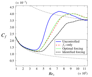
We now evaluate the effectiveness of closed-loop control with the different actuators in delaying transition. Figure 13 shows the friction coefficient  $C_{f}$ and maximum root-mean square (r.m.s.) values for the three evaluated actuators for
 $Tu=3.0\,\%$ and 3.5 %. The corresponding behaviour of the r.m.s. values of the streamwise velocity fluctuation in the
 $(x_{1},x_{2})$ plane are shown in figure 14 for the
 $Tu=3.0\,\%$ case, and in figure 15 four streamwise positions are shown in order to better highlight the effect of the different actuation schemes; similar results are also observed for higher turbulence intensity values.
Friction coefficient and maximum r.m.s. values for the streamwise velocity fluctuation and the different actuation schemes considered in this work. The black dashed lines in the friction coefficient plots give reference values for the laminar and turbulent cases, respectively.

Behaviour of the r.m.s. of the streamwise velocity fluctuation for the uncontrolled and different controlled scenarios evaluated.

The r.m.s. value of the streamwise velocity fluctuations at four streamwise positions as a function of the wall-normal direction for the uncontrolled and different actuators evaluated in this work. Value  $Re_{x}=150\,000$ corresponds to the objective position.

In order to supply a comparison between the energy dispensed by the different actuators and the corresponding savings obtained from the transition delay, the following metric is defined:
 $$\begin{eqnarray}\unicode[STIX]{x1D6F7}=\frac{\unicode[STIX]{x0394}E_{trans}-\text{r.m.s.}(E_{act}(t))}{E_{unc}},\end{eqnarray}$$
where
 $$\begin{eqnarray}\unicode[STIX]{x0394}E_{trans}=E_{unc}-E_{con},\end{eqnarray}$$
 $E_{unc}$ and
 $E_{con}$ supply the mean energy that is dissipated due to friction drag, which can be accounted for by integrating the drag coefficient in the streamwise direction for the uncontrolled and controlled cases, respectively. The term
 $\text{r.m.s.}(E_{act}(t))$ represents the r.m.s. value of the energy consumed due to actuation, which can be computed from the turbulent kinetic energy of the velocity field induced by the actuator,
 $$\begin{eqnarray}E_{act}(t)=a(t)\int _{x_{1_{0}}}^{x_{1_{max}}}\int _{x_{2_{0}}}^{x_{2_{max}}}\int _{x_{3_{0}}}^{x_{3_{max}}}(u^{2}+v^{2}+w^{2})\,\text{d}x_{1}\,\text{d}x_{2}\,\text{d}x_{3}.\end{eqnarray}$$
The metric defined in (5.4) supplies a means of comparison of the efficiency of the actuators in delaying transition: the higher the value of this parameter, the higher the energy gain with respect to actuation, with  $\unicode[STIX]{x1D6F7}=0$ representing an uncontrolled case. It should also be noted that ideal actuators are being considered in this analysis, i.e. no losses are being considered in the generation of the velocity field.
The resulting values for this parameter, along with the corresponding delays in transition and total reduction in drag, obtained by considering the integrated value of  $c_{f}$ are summarized in table 2; the integration was performed from
 $Re_{x}=0.5\times 10^{5}$ to
 $5.5\times 10^{5}$ for the
 $Tu=3.5\,\%$ case and from
 $Re_{x}=1.0\times 10^{5}$ to
 $11.0\times 10^{5}$ for the
 $Tu=3.0\,\%$ case.
Summary of the results obtained in terms of the delay in transition to turbulence and total integrated drag.

It is noticeable that all three actuators lead to significant transition delays with an accompanying reduction in the integrated total drag. For comparison, in the work of Monokrousos et al. (Reference Monokrousos, Brandt, Schlatter and Henningson2008), which also deals with the control of complex disturbances, induced by FST with  $Tu=3.0\,\%$, a transition delay of
 $\unicode[STIX]{x0394}Re_{x}=1.0\times 10^{5}$ is obtained, with a corresponding reduction in the total drag of 5 % to 10 %, using LQG as the control strategy with measurement and actuation strips that extended over a length corresponding to
 $\unicode[STIX]{x0394}Re_{x}=0.80\times 10^{5}$ and
 $\unicode[STIX]{x0394}Re_{x}=0.90\times 10^{5}$, which therefore corresponds to a set-up that is considerably more difficult to implement in an experimental application.
The identified actuator considerably outperforms the other two concerning the delay in transition, a feature observed from the friction coefficient and maximum r.m.s. values in figure 13, which take much longer to increase to values typical of turbulent boundary layers. The r.m.s. values in figure 14 indicate that the effect of the identified actuator is more extended along the wall-normal direction, since, at the position of actuation, there is a significant decrease of r.m.s. levels throughout the boundary layer. Furthermore, the actuation energy of the identified actuator is similar to that of the  $f_{x_{2}}$-only actuator and it is also more robust to the evaluated changes in turbulence intensity, leading also to significant delays in transition for the two evaluated cases. Parameter
 $\unicode[STIX]{x1D6F7}$ indicates that such an actuator presents the most efficient behaviour, leading to the best compromise between transition delay and actuation energy.
As for the optimal forcing actuator, although it is capable of delaying the transition in the two FST intensity cases, it presents the lowest performance in terms of the transition delay. The r.m.s. values indicate that its effect is more localized, which leads to an imperfect cancellation of the incoming streak. These characteristics will be further explored in § 6 by means of an evaluation of the SPOD of the actuation effect. In spite of these characteristics, the optimal forcing actuator leads to the lowest actuation energy for the evaluated cases, approximately one order of magnitude lower than the other two. This is related to the fact that it excites streaks with the highest energy growths and it is therefore capable of leading to a cancellation, specifically at the objective position, with less energy spent. This trend is also present in the parameter  $\unicode[STIX]{x1D6F7}$, which presents an intermediate behaviour between the identified and the
 $f_{x_{2}}$-only actuator.
Finally, the  $f_{x_{2}}$-only actuator presents an intermediate behaviour in terms of the resulting delay in transition. However, it leads to the highest actuation energy, a fact that is observed in the parameter
 $\unicode[STIX]{x1D6F7}$, which becomes negative for the highest
 $Tu$ value, indicating that the actuation is consuming more energy than that saved via transition delay. The results of this section highlight the importance of the methods for actuator design proposed in this work, which allow for much enhanced delays in transition, with lower actuation energies.
(a) Peak of the two-dimensional cross-correlation between estimated and computed LES streamwise velocity fields. The  $x_{1}$ positions of input and output were fixed at 250 and 400, respectively, and the wall-normal position was varied. The dashed line indicates input–output positions at the same wall-normal positions. (b) The r.m.s. values of the streamwise velocity fluctuation at
 $x_{1}=400$ as a function of the wall-normal direction.

Similar trends have been observed for the case of  $Tu=4.5\,\%$, where the observed delays in transition are
 $\unicode[STIX]{x0394}Re_{x}=0.14\times 10^{5}$,
 $0.21\times 10^{5}$ and
 $0.87\times 10^{5}$ for the vertical, optimal and identified forcings, where the last one continued to significantly outperform the other two, leading to compelling delays in transition, even for such a high level of FST. Evaluation of the case
 $Tu=2.5\,\%$ demonstrated that the identified actuator managed to maintain the laminarity of the flow up to
 $Re_{x}=10^{6}$, where a transitional region starts to occur. This case does not transition to turbulence within the evaluated domain size. These results demonstrate that the kernels have been tested under conditions much different from their design points, presenting reasonable performances, which supplies further evidence of the robustness of the control law, identification and optimization methods derived herein.
6 Discussion
Two approaches will be used to better understand the results of the previous section: the SPOD of the open- and closed-loop cases; and the possibility of causal streak cancellation, which is related to the different delays of the actuators in exciting a response in the output. Both of these analyses are related to the fact that the streamwise velocity fluctuations present their peak value above the wall, as will be explored next. All results in this section are shown for the  $Tu=3.0\,\%$ case. Trends for
 $Tu=3.5\,\%$ are similar and will not be displayed for brevity.
6.1 Correlations along the wall-normal direction
We first consider the r.m.s. value of the streamwise velocity fluctuations along the wall-normal direction, given in figure 16. It is noticeable that the maximum value of the r.m.s. is above the wall, located at  $x_{2}\approx 3$. Therefore, in order to obtain a more global effect on the field, the actuator should lead to changes over such higher wall-normal positions rather than in the near-wall region only. Furthermore, the fluctuations at such positions should be predictable given the considered input sensor, which corresponds to measurements of wall-shear stress.
In order to evaluate if the streamwise velocity fluctuations at  $x_{2}=3$ may be predicted from wall measurements, the peak of the two-dimensional cross-correlation between the estimated (obtained via the two-dimensional transfer function) and LES computed fields was calculated as a function of the wall-normal positions of input and output measurements. The streamwise positions were kept at
 $x_{1}=250$ and 400, for input and output, respectively, in accordance with the
 $y$ and
 $z$ measurements. The predicted field was obtained by means of the empirical transfer function approach, as outlined in § 2. The result is shown in figure 16 and demonstrates that there is a strong correlation between wall-shear stress measurements (
 $x_{2,in}\rightarrow 0$) and the streamwise velocity fluctuations up to
 $x_{2}\approx 5$, indicating that the currently considered sensors are adequate for this type of application. Differences are therefore only accountable for the considered actuators, as the method to determine the control law was the same for all of them. In what follows, all the analysis is made with the input sensor corresponding to wall-shear stress.
6.2 Spectral proper orthogonal decomposition in open-loop case
The SPOD is calculated at the objective position,  $x_{1}=400$, in the plane defined by the wall-normal and spanwise coordinates. The decomposition is made per
 $(\unicode[STIX]{x1D714},\unicode[STIX]{x1D6FD}_{k})$ pair and the results shown here will consider
 $(\unicode[STIX]{x1D714},\unicode[STIX]{x1D6FD}_{k})=(0,0.37)$, which corresponds approximately to the most amplified case used in the actuator optimization techniques. The eigenvalues resulting from such decomposition, for the open- and closed-loop cases, considering the different actuation strategies evaluated in this paper, are shown in figure 17.
Eigenvalues of the SPOD modes calculated at position  $x_{1}=400$, for
 $(\unicode[STIX]{x1D714},\unicode[STIX]{x1D6FD}_{k})=(0,0.37)$, for the open- (circles) and closed-loop cases (squares, diamonds and crosses, for the blowing, identified and optimal forcing actuator, respectively).

The first mode is approximately two orders of magnitude higher than the second one, a fact that indicates its dominance in the flow, at the evaluated streamwise position. The three evaluated actuators lead to an attenuation of such a mode in the closed-loop case, along with the subsequent modes higher than two. The identified actuator presents the best performance, leading to a reduction of approximately five times in the magnitude of the first mode eigenvalue.
In order to better distil the effect of each actuator in the flow, simulations were performed without FST and with the actuators with a white-noise time modulation. SPOD was then applied to the resulting data at the position of the objective at the  $(\unicode[STIX]{x1D714},\unicode[STIX]{x1D6FD}_{k})$ pair considered here; the objective is to extract the exact structures that are being excited by the actuators and compare them to the one corresponding to the FST-induced streaks. Figure 18 presents the first SPOD mode for the different cases as a function of the wall-normal direction, for the streamwise velocity fluctuation, which is the velocity component that dominates the fluctuation. The real part of the velocity fluctuation was plotted; the same conclusions hold for the absolute value of the fluctuation.
First SPOD mode for the uncontrolled (solid blue line) and response of different actuation strategies evaluated in this work (red dashed, black dash-dotted and green dotted for the  $f_{x_{2}}$-only, identified and optimal forcing actuator). The evaluation was made at
 $x_{1}=400$, which corresponds to the objective position.

It is clear that, whereas the identified actuator leads to fluctuations in a compelling agreement with the fluctuations inside the boundary layer, the other two excite ‘thinner’ structures with a peak value that occurs closer to the wall than the peak of the streaks inside the boundary layer. This behaviour leads to an imperfect cancellation of the incoming streak. Since a destructive interference is the physical mechanism behind flow control of convectively unstable flows (Sasaki et al. Reference Sasaki, Morra, Fabbiane, Cavalieri, Hanifi and Henningson2018a; Morra et al. Reference Morra, Sasaki, Hanifi, Cavalieri and Henningson2019), the  $f_{x_{2}}$-only and optimal forcing actuators lead to a lower performance in terms of transition delay. As illustrated in figure 15, it is observed that the imperfect cancellation that results from these two actuators leads to a faster recovery of the strongest streak downstream of the position of the objective, in comparison to the identified actuator case.
It should also be noted that the identified actuator presents a peak in its spatial support which is at a higher wall-normal location than the other two (as shown in figure 9); this is probably related to the higher peak of the streak it is identifying inside the flow.
The other two velocity components are not shown, as the streamwise velocity is the foremost contributor to the total energy ( $v$ and
 $w$ correspond to approximately 0.4 % and 0.1 % of the energy at the objective position). Accordingly, it is observed that these two velocity components do not play a significant role in the optimization procedure for obtaining the identified actuator and in the closed-loop behaviour performance.
Behaviour of the impulse responses of the estimated field and different actuators considered here. The measurement was located at the wall (left column) and at  $x_{2}=3$ (right column), and the streamwise position was located at
 $x_{1}=400$, corresponding to the objective of the control law. The colour bar was adjusted for each plot in order to better visualize the behaviour. The dashed line indicates the time delay for the maximum of the impulse response.

6.3 The role of causality in streak cancellation
Figure 19 shows the impulse responses for the estimation – taken between  $(x_{1},x_{2})=(250,0)$, using wall-shear stress as the measurement, and
 $(400,\unicode[STIX]{x1D716})$ or
 $(400,3)$, with streamwise velocity as the output measurement, where
 $\unicode[STIX]{x1D716}$ is the first point of the grid above the wall, using the empirical transfer function – and actuation – taken between
 $(x_{1},x_{2})=(325,0)$ and
 $(400,\unicode[STIX]{x1D716})$ or
 $(400,3)$, considering streamwise velocity as the output measurement. The impulse response for estimation is representative of open-loop disturbances, whereas the one for actuation highlights properties of streaks induced by the control law.
A few characteristics can be observed in figure 19. First, the estimation impulse responses, taken for an input further upstream, present a time delay comparable to the actuation cases, indicating that the group velocity of open-loop streaks is higher than that corresponding to the actuator-induced disturbances. The delay changes between wall and  $x_{2}=3$ measurements, indicating a tilting of the structures, which reach the higher wall-normal position at
 $x_{1}=400$ before reaching the wall at the same streamwise position. Finally, from the time delays of impulse responses, it is inferred that the three actuators induce streaks with different group velocity, with the identified case presenting the highest value and optimal forcing the lowest. The relevance of such time delays for closed-loop control are related to the possibility of a causal cancellation of incoming disturbances, as discussed by Sasaki et al. (Reference Sasaki, Tissot, Cavalieri, Silvestre, Jordan and Biau2018b), and can be summarised, in simplified manner, as follows. Once a given structure is detected by the upstream sensors
 $y$, it is estimated, through the transfer functions in figure 19, that it will reach the downstream objective
 $z$ after a time delay
 $\unicode[STIX]{x1D70F}_{e}$. The actuator should cancel this disturbance, but this cannot occur instantly, since the actuation-induced structures take a time delay
 $\unicode[STIX]{x1D70F}_{a}$ to reach the objective location. If
 $\unicode[STIX]{x1D70F}_{a}<\unicode[STIX]{x1D70F}_{e}$ such cancellation is feasible, whereas in the opposite case it becomes impossible to cancel the incoming streaks; in the latter situation, once an upstream streak is detected in
 $y$, it is already too late to attempt to cancel it in
 $u$.
Considering the time delays for which the impulse response peaks, all actuators are able to generate disturbances that reach the objective position located at the wall before the one related to the estimated field, which can be seen by the characteristic time delays  $\unicode[STIX]{x1D70F}_{a}$, lower than
 $\unicode[STIX]{x1D70F}_{e}$ in figure 19 for all cases. The same is not true when we consider the output at
 $x_{2}=3$, particularly for the optimal forcing actuator. This characteristic will prevent the optimal forcing case of acting where the highest energy of the streak is present, at the objective position.
Streamwise position for the different actuators and estimated field as a function of time. Input positions ( $\unicode[STIX]{x0394}t=0$) were kept fixed at
 $(x_{1},x_{2})=(250,0)$, with wall-shear stress, and
 $(x_{1},x_{2})=(325,0)$, using streamwise velocity, for estimation and actuation cases, respectively. The transverse position of the measured impulse corresponds to (a)
 $x_{2}=\unicode[STIX]{x1D716}$ and (b)
 $x_{2}=3$.

These characteristics are summarized in figure 20, where the streamwise position is given as a function of the time delay for it to be reached for the estimation and each actuator. The delay was considered as the time when the peak value is reached, for each impulse response at the considered position. The slope of lines in the plot can thus be related to the group velocity of disturbances in the open-loop case, given by the estimation transfer function, and of the ones resulting from the three actuators. The values at the wall (considered as  $x_{2}=\unicode[STIX]{x1D716}$) and at
 $x_{2}=3$ are shown in figure 20. The input measurements were considered as
 $x_{1}=250$, for estimation, and
 $x_{2}=325$, for actuation. For all actuators and both wall-normal positions, it is noticeable that the impulse response of the estimation has a higher velocity. Among the three actuators, the identified one leads to structures with higher group velocity, which is particularly clear for the
 $x_{2}=3$ case, the most important one in terms of the energy content of the fluctuations. This higher velocity can be related to generation of streaks at higher wall-normal positions (figure 18), and may further justify the effectiveness of the identified actuator.
It should be noted that when the curve corresponding to the estimated field surpasses those of the impulses, these positions correspond to uncontrollable cases, as the control-induced streaks will reach a downstream position after the incoming structures one wishes to attenuate. The considered objective position of  $x_{1}=400$ is highlighted and the impulse responses of all actuators reach it before the estimated field, which therefore leads to a causal kernel that is capable of the attenuations reported here, which result in a good attenuation of the objective quantity.
However, when one considers the  $x_{2}=3$ case, where most of the fluctuation energy is contained, the streamwise objective position of
 $x_{1}=400$ does not correspond to a causal behaviour when the optimal forcing actuator is considered, which explains why it presents the worst performance among the different spatial supports considered here. The higher group velocity of streaks for larger
 $x_{2}$ prevents a perfect cancellation particularly for the optimal forcing and vertical forcing-only actuators, which present considerably lower values of group velocity.
One could try to compensate for the lower group velocity of the actuator-induced streaks by moving the objective position upstream, closer to the actuator. This would cause all schemes to be causal, both at the wall and at  $x_{2}=3$. However, since the FST is continuously forcing the boundary layer, it is expected that the lower group velocity of the actuator-induced structures, particularly for the vertical force and optimal cases, will eventually play a role in downstream areas of the flow.
7 Conclusions
Three methodologies have been considered for the design of localized actuators for the control of streaky structures, induced by FST. A set-up close to that of practical applications was considered, where a large number of OSS modes was used to model FST. This makes it infeasible to compute individual impulse responses of each disturbance, and an empirical transfer function was derived to obtain a reduced-order model, for which application of a LQG led to control laws. Localized sensors were also considered in the simulation, which further increases the similarity of the work to an actual experimental implementation.
Two of the methods for actuator design corresponded to optimization procedures: either the energy of the actuator-induced disturbances at the position of the objective, or the difference with respect to a previously measured structure between actuator-induced and open-loop disturbances, was considered as the cost function, which was maximized in the first case (leading to an optimal forcing) and minimized in the second (with an identified, tailored actuator that optimally targeted open-loop streaks). The resulting direct–adjoint iteration algorithm was computationally efficient and led to desired results when applied in the nonlinear simulation. A third actuator, corresponding to a vertical forcing only, served as a baseline case, in line with the recent results of Shahriari et al. (Reference Shahriari, Kollert and Hanifi2018) where a ring of plasma actuators was used to excite a vertical body force in a boundary layer.
Closed-loop control with all the actuators led to significant delay in transition, and this was shown to be robust to mild changes in the FST level, a desired characteristic for real-life applications. All three actuators have led to improvements in comparison to other recent works, such as Monokrousos et al. (Reference Monokrousos, Brandt, Schlatter and Henningson2008), and in a more realistic set-up. The optimization/minimization techniques allowed a compelling reduction in the actuator energy (corresponding to the optimal forcing case), or a significant increase in the transition delay (for the identified actuator), estimated to be approximately four times larger than in Monokrousos et al. (Reference Monokrousos, Brandt, Schlatter and Henningson2008), for example. To the best of the authors’ knowledge, this is currently the best performance obtained in terms of transition delay in the control of structures induced by FST in an experimentally implementable set-up. The techniques outlined here for actuator design also allowed significant improvements in the energy saved via transition delay, in comparison to that consumed by actuation, leading to results much further from the break-even point, even for the highest turbulence intensities considered.
Differences between the three cases were understood in terms of the SPOD of estimation and actuation fields, in the open-loop case, which highlighted the dissimilarities between the structures induced by the actuators and the one actually present in a boundary layer. Here, an important difference between the control of TS waves and streaks appears. Whereas, in the former case, any actuator leads to exactly the same TS waves at downstream positions, as these are the only structures in spatial growth, for streaks, a whole family of disturbances can be generated by actuators. It thus becomes important to target precisely the streaks that are actually expected in a given transitional boundary layer, and thus the identified actuator obtains a closed-loop performance superior to the other ones, in terms of the resulting transition delay, since it cancels more accurately the open-loop streaks.
The distinct velocities of structures induced by the three actuators and the streaks induced by the FST, along with the tilting of the structures in the wall-normal direction, also play a role in this type of application, where it may become impossible to obtain a causal cancellation of incoming disturbances, even if the actuator is downstream of the input measurement. Causality will also depend on the wall-normal position under consideration, a feature that had not yet been observed or quantitatively computed.
Finally, an evaluation of the correlations along the wall-normal direction indicated that wall measurements were adequate for the prediction of the output signals. Such a technique allowed similar conclusions to observability tools without the need to perform adjoint simulations. These analysis were possible by means of the empirically calculated impulse responses, which permitted an exploration of the parameters of the problem, reducing the number of required nonlinear simulations.
Concerning the design of actuators for experimental applications, it was shown that a vertical forcing only, which is currently possible to implement, should be adequate for the control of streaky structures. Better results may be obtained in terms of both the transition delay and the energy budget of actuation when access to the open-loop data is available prior to the design of the actuator, where the methods outlined here for the evaluation of the forcing and optimization should aid in the design of new actuators for flow control, which is currently a challenge in the flow control community.
Acknowledgements
The authors would like to acknowledge the VINNOVA Projects PreLaFlowDes and SWE-DEMO and the Swedish–Brazilian Research and Innovation Centre CISB for funding. Moreover, part of this work was performed during an exchange programme at KTH, for which K.S. received a scholarship from Capes, project no. 88881.132008/2016-01. K.S. is also funded by a scholarship from FAPESP, grant no. 2016/25187-4. A.V.G.C. was supported by a CNPq grant no. 310523/2017-6 and FAPESP grant no. 2019/13393-7. The simulations were performed on resources provided by the Swedish National Infrastructure for Computing (SNIC) at NSC, HPC2N and PDC.
Appendix A. Calculation of spectral proper orthogonal decomposition modes from data
We briefly outline the approach to compute SPOD modes from snapshots taken from a simulation or experimental data. As in the main body of the paper,  $\boldsymbol{q}(x,y,z,t)=(u(x_{1},x_{2},x_{3},t),v(x_{1},x_{2},x_{3},t),w(x_{1},x_{2},x_{3},t))$, which is then Fourier-transformed from
 $x_{3}$ to
 $\unicode[STIX]{x1D6FD}_{k}$,
 $$\begin{eqnarray}\hat{\boldsymbol{q}}(x_{1},x_{2},\unicode[STIX]{x1D6FD},t)=\int _{-x_{2_{max}}/2}^{x_{2_{max}}/2}\boldsymbol{q}(x_{1},x_{2},x_{3},t)\text{e}^{-\text{i}\unicode[STIX]{x1D6FD}\unicode[STIX]{x1D701}}\,\text{d}\unicode[STIX]{x1D701}.\end{eqnarray}$$
The spanwise direction is discretized and the continuous Fourier transform becomes a discrete Fourier transform (DFT), which is evaluated at the discrete wavenumbers  $\unicode[STIX]{x1D6FD}_{k}$. Given the periodicity of this coordinate, the DFT is regarded as the discretization of the coefficients of the corresponding Fourier series.
Considering now the discretization in time, the quantity  $\hat{\boldsymbol{q}}_{k}(\unicode[STIX]{x1D6FD}_{k})$ represents the instantaneous state of
 $\hat{\boldsymbol{q}}(\unicode[STIX]{x1D6FD}_{k},t)$. If a total number of
 $N$ snapshots is used, the signal may be regarded as
 $$\begin{eqnarray}\hat{\unicode[STIX]{x1D64C}}(\unicode[STIX]{x1D6FD}_{k})=[\hat{\boldsymbol{q}}_{1}(\unicode[STIX]{x1D6FD}_{k})\quad \hat{\boldsymbol{q}}_{2}(\unicode[STIX]{x1D6FD}_{k})\quad \ldots \quad \hat{\boldsymbol{q}}_{N}(\unicode[STIX]{x1D6FD}_{k})],\end{eqnarray}$$
where  $\hat{\unicode[STIX]{x1D64C}}(\unicode[STIX]{x1D6FD}_{k})$ is
 $N_{s}\times N$, with
 $N_{s}$ representing the number of spatial grid points times the number of physical quantities considered (in this case, the three velocity components and pressure). Application of the DFT directly into the lines of matrix
 $\hat{\unicode[STIX]{x1D64C}}(\unicode[STIX]{x1D6FD}_{k})$ should not be performed, as the result will not converge with the number of snapshots (Bendat & Piersol Reference Bendat and Piersol2011), and the order of magnitude of the error could be as high as the corresponding magnitude of the spectrum. Therefore, in order to obtain converged values of the spectral density, for calculation of the spectral density tensor, it is necessary to average the spectra over multiple realizations of the flow. This may be accomplished by application of Welch’s method (Welch Reference Welch1967).
Start by partitioning the full signal into  $N_{b}$ blocks, each with
 $N_{f}$ elements; the
 $n$th block is then given as
 $$\begin{eqnarray}\hat{\unicode[STIX]{x1D64C}}^{(n)}(\unicode[STIX]{x1D6FD}_{k})=[\hat{\boldsymbol{q}}_{1}^{(n)}(\unicode[STIX]{x1D6FD}_{k})\quad \hat{\boldsymbol{q}}_{2}^{(n)}(\unicode[STIX]{x1D6FD}_{k})\quad \ldots \quad \hat{\boldsymbol{q}}_{N_{f}}^{(n)}(\unicode[STIX]{x1D6FD}_{k})],\end{eqnarray}$$
such that each block can be regarded as a realization of the flow. Overlapping the blocks with adjacent elements is possible and allows a higher number of blocks for the same length of the original signal, permitting a faster convergence of the statistics. The  $k$th entry in the
 $n$th block is then given as
 $\hat{\boldsymbol{q}}_{k}^{(n)}(\unicode[STIX]{x1D6FD}_{k})=\hat{\boldsymbol{q}}_{k+(n-1)(N_{f}-N_{o})}(\unicode[STIX]{x1D6FD}_{k})$, where
 $N_{o}$ is the number of overlapping snapshots. The DFT is then calculated at each block,
 $$\begin{eqnarray}\hat{\hat{\unicode[STIX]{x1D64C}}}^{(n)}(\unicode[STIX]{x1D6FD}_{k})=[\hat{\hat{\boldsymbol{q}}}_{1}^{(n)}(\unicode[STIX]{x1D6FD}_{k})\quad \hat{\hat{\boldsymbol{q}}}_{2}^{(n)}(\unicode[STIX]{x1D6FD}_{k})\quad \ldots \quad \hat{\hat{\boldsymbol{q}}}_{N_{f}}^{(n)}(\unicode[STIX]{x1D6FD}_{k})],\end{eqnarray}$$
where the  $k$th element of the block is then given as
 $$\begin{eqnarray}\hat{\hat{\boldsymbol{q}}}_{k}^{(n)}(\unicode[STIX]{x1D6FD}_{k})=\frac{1}{\sqrt{N_{f}}}\mathop{\sum }_{j=1}^{N_{f}}w_{j}\hat{\hat{\boldsymbol{q}}}_{j}^{(n)}(\unicode[STIX]{x1D6FD}_{k})\text{e}^{-2\unicode[STIX]{x03C0}\text{i}(k-1)[(j-1)/N_{f}]},\end{eqnarray}$$
with  $k=1,\ldots ,N_{f}$ and
 $n=1,\ldots ,N_{b}$. Equation (A 5) represents the discrete Fourier transform of the block, with the addition of the weights
 $w_{j}$, which allow the application of a window function, used to reduce spectral leakage due to the non-periodicity of the block. The normalization factor
 $1/N_{f}$ ensures the transform is unitary for a square window. Here
 $\hat{\hat{\boldsymbol{q}}}_{k}^{(n)}(\unicode[STIX]{x1D6FD}_{k})$ is the
 $k$th element of the DFT of the
 $n$th block, with a corresponding frequency
 $\unicode[STIX]{x1D714}_{k}$,
 $$\begin{eqnarray}\unicode[STIX]{x1D714}_{k}=2\unicode[STIX]{x03C0}\frac{k-1}{n\unicode[STIX]{x0394}T},\quad k\leqslant n/2,\end{eqnarray}$$
or
 $$\begin{eqnarray}\unicode[STIX]{x1D714}_{k}=2\unicode[STIX]{x03C0}\frac{k-1-n}{n\unicode[STIX]{x0394}t},\quad k>n/2.\end{eqnarray}$$
Finally, the cross-spectral density tensor  $\unicode[STIX]{x1D71E}(\boldsymbol{x},\boldsymbol{x}^{\prime },\unicode[STIX]{x1D714},\unicode[STIX]{x1D6FD}_{k})$ can be estimated at a frequency
 $\unicode[STIX]{x1D714}_{k}$ and spanwise wavenumber
 $\unicode[STIX]{x1D6FD}_{k}$ by averaging the blocks,
 $$\begin{eqnarray}\unicode[STIX]{x1D71E}_{\unicode[STIX]{x1D714}_{k}}(\unicode[STIX]{x1D6FD}_{k})=\frac{\unicode[STIX]{x0394}t}{sN_{b}}\mathop{\sum }_{n=1}^{N_{b}}\hat{\hat{\boldsymbol{q}}}_{k}^{(n)}(\unicode[STIX]{x1D6FD}_{k})(\hat{\hat{\boldsymbol{q}}}_{k}^{(n)}(\unicode[STIX]{x1D6FD}_{k}))^{\ast },\end{eqnarray}$$
and  $s=\sum _{j=1}^{N_{f}}w_{j}^{2}$. Each Fourier coefficient at a frequency
 $\unicode[STIX]{x1D714}_{k}$ for each block, at a given
 $\unicode[STIX]{x1D6FD}_{k}$, can be arranged in a matrix form,
 $$\begin{eqnarray}\hat{\hat{\unicode[STIX]{x1D64C}}}_{\unicode[STIX]{x1D714}_{k}}(\unicode[STIX]{x1D6FD}_{k})=\sqrt{k}[\hat{\hat{\boldsymbol{q}}}_{k}^{(1)}(\unicode[STIX]{x1D6FD}_{k})\quad \hat{\hat{\boldsymbol{q}}}_{k}^{(2)}(\unicode[STIX]{x1D6FD}_{k})\quad \ldots \quad \hat{\hat{\boldsymbol{q}}}_{k}^{(N_{b})}(\unicode[STIX]{x1D6FD}_{k})],\end{eqnarray}$$
where  $k=\unicode[STIX]{x0394}t/(sN_{b})$ and
 $\hat{\hat{\unicode[STIX]{x1D64C}}}_{\unicode[STIX]{x1D714}_{k}}(\unicode[STIX]{x1D6FD}_{k})$ is
 $N\times N_{b}$. The cross-spectral density tensor is then written compactly as
 $$\begin{eqnarray}\unicode[STIX]{x1D71E}_{\unicode[STIX]{x1D714}_{k}}(\unicode[STIX]{x1D6FD}_{k})=\hat{\hat{\unicode[STIX]{x1D64C}}}_{\unicode[STIX]{x1D714}_{k}}(\unicode[STIX]{x1D6FD}_{k})(\hat{\hat{\unicode[STIX]{x1D64C}}}_{\unicode[STIX]{x1D714}_{k}}(\unicode[STIX]{x1D6FD}_{k}))^{\ast }.\end{eqnarray}$$
The calculation of the cross-spectral density tensor then converges as the number of blocks and snapshots at each block are increased together (Bendat & Piersol Reference Bendat and Piersol2011).
Defining the positive-define Hermitian matrix  $\unicode[STIX]{x1D652}$,
 $N\times N$, to account for the weight and the numerical quadrature for performing an integral on a discrete grid, the SPOD eigenvalue problem reduces to an
 $N\times N$ matrix eigenvalue problem, at each frequency and transverse wavenumber,
 $$\begin{eqnarray}\unicode[STIX]{x1D71E}_{\unicode[STIX]{x1D714}_{k}}(\unicode[STIX]{x1D6FD}_{k})\unicode[STIX]{x1D652}\unicode[STIX]{x1D713}_{\unicode[STIX]{x1D714}_{k}}(\unicode[STIX]{x1D6FD}_{k})=\unicode[STIX]{x1D713}_{\unicode[STIX]{x1D714}_{k}}(\unicode[STIX]{x1D6FD}_{k})\unicode[STIX]{x1D706}_{\unicode[STIX]{x1D714}_{k}}(\unicode[STIX]{x1D6FD}_{k}).\end{eqnarray}$$
The SPOD modes are then given in the columns of  $\unicode[STIX]{x1D713}_{\unicode[STIX]{x1D714}_{k}}(\unicode[STIX]{x1D6FD}_{k})$, ranked according to their corresponding eigenvalues, which are in the diagonal matrix
 $\unicode[STIX]{x1D713}_{\unicode[STIX]{x1D714}_{k}}(\unicode[STIX]{x1D6FD}_{k})$.
Appendix B. Derivation of the optimization schemes
In this section, the two schemes for the calculation of the actuators considered in §§ 4.2 and 4.3 will be outlined. We follow the works of Andersson et al. (Reference Andersson, Berggren and Henningson1999) and Levin & Henningson (Reference Levin and Henningson2003) in a scheme appropriate for algebraically growing disturbances along the streamwise direction, for a slowly divergent mean flow. The pressure and velocity fluctuations follow the boundary layer equations, which, written in matrix form, are given as
 $$\begin{eqnarray}\boldsymbol{{\mathcal{A}}}\hat{\boldsymbol{q}}+\boldsymbol{{\mathcal{B}}}\frac{\unicode[STIX]{x2202}\hat{\boldsymbol{q}}}{\unicode[STIX]{x2202}x_{2}}+\boldsymbol{{\mathcal{C}}}\frac{\unicode[STIX]{x2202}^{2}\hat{\boldsymbol{q}}}{\unicode[STIX]{x2202}x_{2}^{2}}+\boldsymbol{{\mathcal{D}}}\frac{\unicode[STIX]{x2202}\hat{\boldsymbol{q}}}{\unicode[STIX]{x2202}x_{1}}=\hat{\unicode[STIX]{x1D641}},\end{eqnarray}$$
where  $\hat{\unicode[STIX]{x1D641}}=(0,\hat{F}_{x_{1}},\hat{F}_{x_{2}},\hat{F}_{x_{3}})$ is a forcing applied in the three directions and
 $\hat{\boldsymbol{q}}=(\hat{u} ,\hat{v},{\hat{w}},\hat{p})$, and the hat indicates quantities given in the
 $(\unicode[STIX]{x1D714},\unicode[STIX]{x1D6FD})$ domain. Equation (B 1) results from the application of the ansatz
 $\boldsymbol{q}=\hat{\boldsymbol{q}}(x,y)\text{e}^{(\text{i}\unicode[STIX]{x1D6FD}z-\text{i}\unicode[STIX]{x1D714}_{t})}$ into the linearized Navier–Stokes equations. The operators are then given as
 $$\begin{eqnarray}\displaystyle & \displaystyle \boldsymbol{{\mathcal{A}}}=\left(\begin{array}{@{}cccc@{}}0 & 0 & \text{i}\unicode[STIX]{x1D6FD} & 0\\ -\text{i}\unicode[STIX]{x1D714}+\unicode[STIX]{x1D6FD}^{2}/Re+\text{d}U/\text{d}x_{1} & \text{d}U/\text{d}x_{2} & 0 & 0\\ 0 & -\text{i}\unicode[STIX]{x1D714}+\unicode[STIX]{x1D6FD}^{2}/Re+\text{d}V/\text{d}x_{2} & 0 & 0\\ 0 & 0 & -\text{i}\unicode[STIX]{x1D714}+\unicode[STIX]{x1D6FD}^{2}/Re & \text{i}\unicode[STIX]{x1D6FD}\end{array}\right)\!,\quad \quad & \displaystyle\end{eqnarray}$$
 $$\begin{eqnarray}\displaystyle & \displaystyle \boldsymbol{{\mathcal{B}}}=\left(\begin{array}{@{}cccc@{}}0 & \unicode[STIX]{x1D644} & 0 & 0\\ V & 0 & 0 & 0\\ 0 & V & 0 & \unicode[STIX]{x1D644}\\ 0 & 0 & V & \unicode[STIX]{x1D644}\\ \end{array}\right)\!, & \displaystyle\end{eqnarray}$$
 $$\begin{eqnarray}\displaystyle & \displaystyle \boldsymbol{{\mathcal{C}}}=\left(\begin{array}{@{}cccc@{}}0 & 0 & 0 & 0\\ -\unicode[STIX]{x1D644}/Re & 0 & 0 & 0\\ 0 & -\unicode[STIX]{x1D644}/Re & 0 & 0\\ 0 & 0 & -\unicode[STIX]{x1D644}/Re & 0\\ \end{array}\right)\!, & \displaystyle\end{eqnarray}$$
 $$\begin{eqnarray}\displaystyle & \displaystyle \boldsymbol{{\mathcal{D}}}=\left(\begin{array}{@{}cccc@{}}\unicode[STIX]{x1D644} & 0 & 0 & 0\\ U & 0 & 0 & 0\\ 0 & U & 0 & 0\\ 0 & 0 & U & 0\\ \end{array}\right)\!, & \displaystyle\end{eqnarray}$$
where  $U$ and
 $V$ are the mean velocity components in the streamwise and wall-normal direction, respectively, and
 $\unicode[STIX]{x1D644}$ is the identity matrix. The same non-dimensionalizations as in the remainder of the paper are considered here. It should also be noted that the streamwise wavenumber, normally referred to as
 $\unicode[STIX]{x1D6FC}$, is not present in these equations, as there will be no exponential dependence of the fluctuations and all streamwise variation is to be absorbed in
 $\hat{\boldsymbol{q}}(x_{1},x_{2},\unicode[STIX]{x1D714},\unicode[STIX]{x1D6FD})$, which implies that TS waves are not considered in this ansatz. These equations are appropriate for algebraically growing disturbances, such as the streaky structures induced by the FST.
Equation (B 1) can be written in compact form as
 $$\begin{eqnarray}{\mathcal{L}}\hat{\boldsymbol{q}}=\hat{\unicode[STIX]{x1D641}},\end{eqnarray}$$
where the spatial, frequency and wavenumber dependences have been absorbed into  ${\mathcal{L}}$ as
 $$\begin{eqnarray}{\mathcal{L}}=\boldsymbol{{\mathcal{A}}}+\boldsymbol{{\mathcal{B}}}D_{x_{2}}+\boldsymbol{{\mathcal{C}}}D_{x_{2}}^{2}+\boldsymbol{{\mathcal{D}}}D_{x_{1}},\end{eqnarray}$$
where the derivative operators  $D_{x_{2}}$ and
 $D_{x_{1}}$ represent discretized derivative operations in the wall-normal and streamwise directions, respectively.
Equation (B 1) is integrated in the streamwise direction using a first- or second-order explicit Euler method. We solve the problem subject to an initial condition at  $x_{1}=0$, and, since the equation is parabolic, downstream spatial marching can be performed. The discretization over the wall-normal direction is made by means of Chebyshev polynomials considering 300 points. Dirichlet boundary conditions are applied to the velocity components at the wall and at
 $x_{2}\rightarrow \infty$.
The objective is to minimize a cost function that considers the difference between the calculated fluctuation, at the objective position, and the SPOD of the field in the open-loop case. A similar approach has been used by Tissot et al. (Reference Tissot, Zhang, Lajús, Cavalieri and Jordan2017) to identify forcing terms in a turbulent jet. The considered cost function is then
 $$\begin{eqnarray}E_{f}=\frac{1}{2}\int _{0}^{\infty }\Vert \hat{\boldsymbol{q}}-\hat{\boldsymbol{q}}_{SPOD}\Vert ^{2}|_{x_{1}=x_{1_{f}}}\,\text{d}x_{2}.\end{eqnarray}$$
It should be noted that, by considering  $\hat{\boldsymbol{q}}_{SPOD}=0$ and performing a maximization, rather than a minimization, the usual procedure to obtain the optimal forcing is recovered. This will be treated as a particular case of this procedure.
We then follow the approach of Pralits et al. (Reference Pralits, Airiau, Hanifi and Henningson2000) by defining an extended Lagrangian functional that includes the cost function and the constraint, which is given in terms of (B 6), with the addition of a Lagrange multiplier, which plays the role of the adjoint variable,  $\hat{\boldsymbol{q}}^{\ast }$:
 $$\begin{eqnarray}J=E_{f}-Re(\langle \hat{\boldsymbol{q}}^{\ast },{\mathcal{L}}\hat{\boldsymbol{q}}-\hat{\unicode[STIX]{x1D641}}\rangle ).\end{eqnarray}$$
The angle brackets represent the inner product, which is defined for two arbitrary functions as
 $$\begin{eqnarray}\langle \unicode[STIX]{x1D719},\unicode[STIX]{x1D713}\rangle =\int _{x_{1_{0}}}^{x_{1_{f}}}\int _{0}^{\infty }\overline{\unicode[STIX]{x1D719}}(x_{1},x_{2})\unicode[STIX]{x1D713}(x_{1},x_{2})\,\text{d}x_{2}\,\text{d}x_{1}.\end{eqnarray}$$
We then take the variation of (B 9), which leads to
 $$\begin{eqnarray}\unicode[STIX]{x1D6FF}J=\int _{0}^{\infty }(\overline{\hat{\boldsymbol{q}}}-\overline{\hat{\boldsymbol{q}}_{SPOD}})|_{x_{1}=x_{1_{f}}}\unicode[STIX]{x1D6FF}\hat{\boldsymbol{q}}\,\text{d}x_{2}-\langle \hat{\boldsymbol{q}}^{\ast },{\mathcal{L}}\unicode[STIX]{x1D6FF}\hat{\boldsymbol{q}}-\unicode[STIX]{x1D6FF}\hat{\unicode[STIX]{x1D641}}\rangle -\langle \unicode[STIX]{x1D6FF}\hat{\boldsymbol{q}}^{\ast },{\mathcal{L}}\hat{\boldsymbol{q}}-\hat{\unicode[STIX]{x1D641}}\rangle ,\end{eqnarray}$$
corresponding to the sensitivity of the Lagrangian functional to infinitesimal changes,  $\unicode[STIX]{x1D6FF}\hat{\boldsymbol{q}}$,
 $\unicode[STIX]{x1D6FF}\hat{\boldsymbol{F}}$ and
 $\unicode[STIX]{x1D6FF}\hat{\boldsymbol{q}}^{\ast }$. When the variation becomes zero, the Lagrangian is minimized or maximized. The third term
 $\langle \unicode[STIX]{x1D6FF}\hat{\boldsymbol{q}}^{\ast },{\mathcal{L}}\hat{\boldsymbol{q}}-\hat{\unicode[STIX]{x1D641}}\rangle$ is equal to zero, given that the state equation in (B 6) is satisfied, as desired. Zeroing the second term will result in the adjoint problem and corresponding boundary and initial conditions, as follows.
The operators are moved to the right side of the inner product by considering the following property of the adjoint,
 $$\begin{eqnarray}\langle \hat{\boldsymbol{q}}^{\ast },\boldsymbol{{\mathcal{A}}}\hat{\boldsymbol{q}}\rangle =\langle \boldsymbol{{\mathcal{A}}}^{\ast }\hat{\boldsymbol{q}}^{\ast },\hat{\boldsymbol{q}}\rangle ,\end{eqnarray}$$
where the star  $\ast$, refers to a conjugate transpose, when applied to a matrix operator. The derivatives are moved from the direct to the adjoint problem by integrations by parts. We then obtain
 $$\begin{eqnarray}\langle \hat{\boldsymbol{q}}^{\ast },{\mathcal{L}}\unicode[STIX]{x1D6FF}\hat{\boldsymbol{q}}-\unicode[STIX]{x1D6FF}\hat{\unicode[STIX]{x1D641}}\rangle =\langle (\boldsymbol{{\mathcal{A}}}^{\ast }-\boldsymbol{{\mathcal{B}}}_{x_{2}}^{\ast }-\boldsymbol{{\mathcal{D}}}_{x_{1}}^{\ast })\hat{\boldsymbol{q}}^{\ast }-\boldsymbol{{\mathcal{B}}}^{\ast }\hat{\boldsymbol{q}}_{x_{2}}^{\ast }+\boldsymbol{{\mathcal{C}}}^{\ast }\hat{\boldsymbol{q}}_{x_{2}x_{2}}^{\ast }-\boldsymbol{{\mathcal{D}}}^{\ast }\hat{\boldsymbol{q}}_{x_{1}}^{\ast },\hat{\boldsymbol{q}}\rangle -\langle \hat{\boldsymbol{q}}^{\ast },\unicode[STIX]{x1D6FF}\hat{\unicode[STIX]{x1D641}}\rangle +\text{b.c.},\end{eqnarray}$$
where the subscripts  $x_{1}$ and
 $x_{2}$ indicate that the corresponding operator has been derived with respect to
 $x_{1}$ or
 $x_{2}$. Setting this to zero for arbitrary
 $\unicode[STIX]{x1D6FF}\hat{\boldsymbol{q}}$ leads to the adjoint boundary layer equations, given by
 $$\begin{eqnarray}(\boldsymbol{{\mathcal{A}}}^{\ast }-\boldsymbol{{\mathcal{B}}}_{x_{2}}^{\ast }-\boldsymbol{{\mathcal{D}}}_{x_{1}}^{\ast })\hat{\boldsymbol{q}}^{\ast }-\boldsymbol{{\mathcal{B}}}^{\ast }\hat{\boldsymbol{q}}_{x_{2}}^{\ast }+\boldsymbol{{\mathcal{C}}}^{\ast }\hat{\boldsymbol{q}}_{x_{2}x_{2}}^{\ast }-\boldsymbol{{\mathcal{D}}}^{\ast }\hat{\boldsymbol{q}}_{x_{1}}^{\ast }=0,\end{eqnarray}$$
where the subscripts  $x_{1}$ and
 $x_{2}$ represent derivatives along the corresponding directions.
The term b.c., standing for boundary conditions, corresponds to four integrals. Once set to zero, this term will supply the boundary conditions for the adjoint boundary layer equations. Writing the first three explicitly, we have
 $$\begin{eqnarray}\displaystyle & \displaystyle \int _{x_{1_{0}}}^{x_{1_{f}}}\langle \boldsymbol{{\mathcal{B}}}^{\ast }\hat{\boldsymbol{q}}^{\ast },\unicode[STIX]{x1D6FF}\hat{\boldsymbol{q}}\rangle |_{0}^{x_{2_{max}}}\,\text{d}x=\int _{x_{1_{0}}}^{x_{1_{f}}}(V\overline{\hat{u} }^{\ast }\unicode[STIX]{x1D6FF}\hat{u} +(\overline{\hat{p}}^{\ast }+V\overline{\hat{v}}^{\ast })\unicode[STIX]{x1D6FF}\hat{v}+V\overline{{\hat{w}}}^{\ast }\unicode[STIX]{x1D6FF}{\hat{w}}+\overline{\hat{v}}^{\ast }\unicode[STIX]{x1D6FF}\hat{p})|_{0}^{x_{2_{max}}}\,\text{d}x_{1}=0, & \displaystyle \nonumber\\ \displaystyle & & \displaystyle\end{eqnarray}$$
 $$\begin{eqnarray}\displaystyle & \displaystyle \int _{x_{1_{0}}}^{x_{1_{f}}}\langle \boldsymbol{{\mathcal{C}}}^{\ast }\hat{\boldsymbol{q}}^{\ast },\unicode[STIX]{x1D6FF}\hat{\boldsymbol{q}}_{y}\rangle |_{0}^{x_{2_{max}}}\,\text{d}x_{1}=\int _{x_{1_{0}}}^{x_{1_{f}}}(-\overline{\hat{u} }^{\ast }\unicode[STIX]{x1D6FF}\hat{u} _{x_{2}}-\overline{\hat{v}}^{\ast }\unicode[STIX]{x1D6FF}\hat{v}_{x_{2}}-\overline{{\hat{w}}}^{\ast }\unicode[STIX]{x1D6FF}{\hat{w}}_{x_{2}})|_{0}^{x_{2_{max}}}\,\text{d}x_{1}=0,\qquad & \displaystyle\end{eqnarray}$$
 $$\begin{eqnarray}\displaystyle & \displaystyle \int _{x_{1_{0}}}^{x_{1_{f}}}\langle \boldsymbol{{\mathcal{C}}}^{\ast }\hat{\boldsymbol{q}}_{x_{2}}^{\ast },\unicode[STIX]{x1D6FF}\hat{\boldsymbol{q}}\rangle |_{0}^{x_{2_{max}}}\,\text{d}x_{1}=\int _{x_{1_{0}}}^{x_{1_{f}}}(-\overline{\hat{u} }_{x_{2}}^{\ast }\unicode[STIX]{x1D6FF}\hat{u} -\overline{\hat{v}}_{x_{2}}^{\ast }\unicode[STIX]{x1D6FF}\hat{v}-\overline{{\hat{w}}}_{x_{2}}^{\ast }\unicode[STIX]{x1D6FF}{\hat{w}})|_{0}^{x_{2_{max}}}\,\text{d}x_{1}=0.\qquad & \displaystyle\end{eqnarray}$$
The boundary conditions are then given as
 $$\begin{eqnarray}\overline{\hat{u} }^{\ast }=\overline{\hat{v}}^{\ast }=\overline{{\hat{w}}}^{\ast }|_{x_{2}=0}=0\end{eqnarray}$$
and
 $$\begin{eqnarray}\overline{\hat{u} }^{\ast }=\overline{\hat{v}}^{\ast }=\overline{{\hat{w}}}^{\ast }|_{x_{2}=x_{2_{max}}}=0.\end{eqnarray}$$
Finally, zeroing the fourth boundary term, which comes from the streamwise derivative, supplies the initial condition for the adjoint variables, set in the final point of the domain, which corresponds to the objective position
 $$\begin{eqnarray}\int _{0}^{\infty }((\overline{\hat{p}}^{\ast }+U\overline{\hat{u} }^{\ast })\unicode[STIX]{x1D6FF}\hat{u} +U\overline{\hat{v}}^{\ast }\unicode[STIX]{x1D6FF}\hat{v}+U\overline{{\hat{w}}}^{\ast }\unicode[STIX]{x1D6FF}{\hat{w}})|_{x_{1_{0}}}^{x_{1_{f}}}\,\text{d}x_{2}=\int _{0}^{\infty }(\overline{\hat{\boldsymbol{q}}}-\overline{\hat{\boldsymbol{q}}_{SPOD}})|_{x_{1}=x_{1_{f}}}\unicode[STIX]{x1D6FF}\hat{\boldsymbol{q}}\,\text{d}x_{2}.\end{eqnarray}$$
The initial conditions for the direct problem are zero and at the final point of calculation  $x_{1}=x_{1_{f}}$, which therefore implies that
 $$\begin{eqnarray}\displaystyle & \displaystyle \hat{u} ^{\ast }(x_{1}=x_{1_{f}})=\hat{u} (x_{1}=x_{1_{f}})-\hat{u} _{SPOD}(x_{1}=x_{1_{f}}), & \displaystyle\end{eqnarray}$$
 $$\begin{eqnarray}\displaystyle & \displaystyle \hat{v}^{\ast }(x_{1}=x_{1_{f}})=\hat{v}(x_{1}=x_{1_{f}})-\hat{v}_{SPOD}(x_{1}=x_{1_{f}}), & \displaystyle\end{eqnarray}$$
 $$\begin{eqnarray}\displaystyle & \displaystyle {\hat{w}}^{\ast }(x_{1}=x_{1_{f}})={\hat{w}}(x_{1}=x_{1_{f}})-{\hat{w}}_{SPOD}(x_{1}=x_{1_{f}}), & \displaystyle\end{eqnarray}$$
and  $\hat{p}^{\ast }(x_{1}=x_{1_{f}})=0$.
Finally, the variation of  $J$ remains with a single term:
 $$\begin{eqnarray}\unicode[STIX]{x1D6FF}J=\langle \hat{\boldsymbol{q}}^{\ast },\unicode[STIX]{x1D6FF}\hat{\unicode[STIX]{x1D641}}\rangle =\int _{x_{1_{0}}}^{x_{1_{f}}}\int _{0}^{\infty }\overline{\hat{q}^{\ast }}(x_{1},x_{2})\unicode[STIX]{x1D6FF}\hat{\unicode[STIX]{x1D641}}\,\text{d}x_{2}\,\text{d}x_{1}.\end{eqnarray}$$
Since no source terms are being considered on the wall, the variation of  $J$ may be written in terms of the gradient of the objective with respect to the forcing term:
 $$\begin{eqnarray}\unicode[STIX]{x1D6FF}J=\int _{x_{1_{0}}}^{x_{1_{f}}}\int _{0}^{\infty }\overline{\unicode[STIX]{x1D735}}_{\unicode[STIX]{x1D641}}E_{f}\unicode[STIX]{x1D6FF}\hat{\unicode[STIX]{x1D641}}\,\text{d}x_{2}\,\text{d}x_{1},\end{eqnarray}$$
which implies that
 $$\begin{eqnarray}\unicode[STIX]{x1D735}_{\unicode[STIX]{x1D641}}E_{f}=\hat{\boldsymbol{q}}^{\ast }.\end{eqnarray}$$
Equation (B 26) states that the gradient of the parameter to be optimized with respect to the forcing is equal to the adjoint variable and it therefore permits one to find the desired forcing by means of a gradient optimization scheme:
 $$\begin{eqnarray}\hat{\unicode[STIX]{x1D641}}^{n+1}=\hat{\unicode[STIX]{x1D641}}^{n}+\unicode[STIX]{x1D6FE}\unicode[STIX]{x1D735}_{\unicode[STIX]{x1D641}}E_{f}\unicode[STIX]{x1D6FF}\hat{\unicode[STIX]{x1D641}}^{n}.\end{eqnarray}$$
The cost function, equation (B 8), will define the two actuators considered in this paper. If one considers  $\hat{\boldsymbol{q}}_{SPOD}=0$, the optimization procedure will obtain the highest energy, and by setting
 $\unicode[STIX]{x1D6FE}>0$, this is referred to as the optimal forcing. If
 $\hat{\boldsymbol{q}}_{SPOD}$ is taken as the SPOD of the actual field, induced by the FST in the open-loop case, then we take
 $\unicode[STIX]{x1D6FE}<0$, corresponding to a minimization, which is referred to as the identified actuator, which will target the specific structure inside the boundary layer. Other than the value of
 $\unicode[STIX]{x1D706}$, the only change between the two methods is the terminal condition for the adjoint, equations (B 21)–(B 23).
The algorithm for the power iterations using the adjoint can then be written as follows:
(a) Start with a random force field and zero initial conditions and integrate the direct problem, equation (B 1), from the position of actuation until the objective.
(b) Take the final condition for the adjoint problem from (B 21)–(B 22) and integrate equation (B 14) backwards, from the position of the objective up to the position of actuation.
(c) Update the forcing field using (B 27) and calculate the cost function (B 8). Evaluate the convergence and either repeat from the first step or terminate the method.
It could be advantageous to work with an actuator that is concentrated in the streamwise direction. To obtain this result, a Gaussian mask of the type
 $$\begin{eqnarray}M(x_{1})=\exp (-(x_{1}-x_{1_{0}})^{2}/L_{x_{1}}^{2})\end{eqnarray}$$
may be used to multiply the forcing in (B 27) at each iteration. This leads to a slower convergence of the algorithm; however, it was not found to be prohibitive.
Finally, the spanwise spatial support of the forcings was chosen to be also in the form of a Gaussian, which is multiplied by the final result of the forcing. The values of  $(\unicode[STIX]{x1D714},\unicode[STIX]{x1D6FD})$ were chosen in accordance with the most amplified structures in the flow.


 Open access

