2. Governing equations and boundary conditions

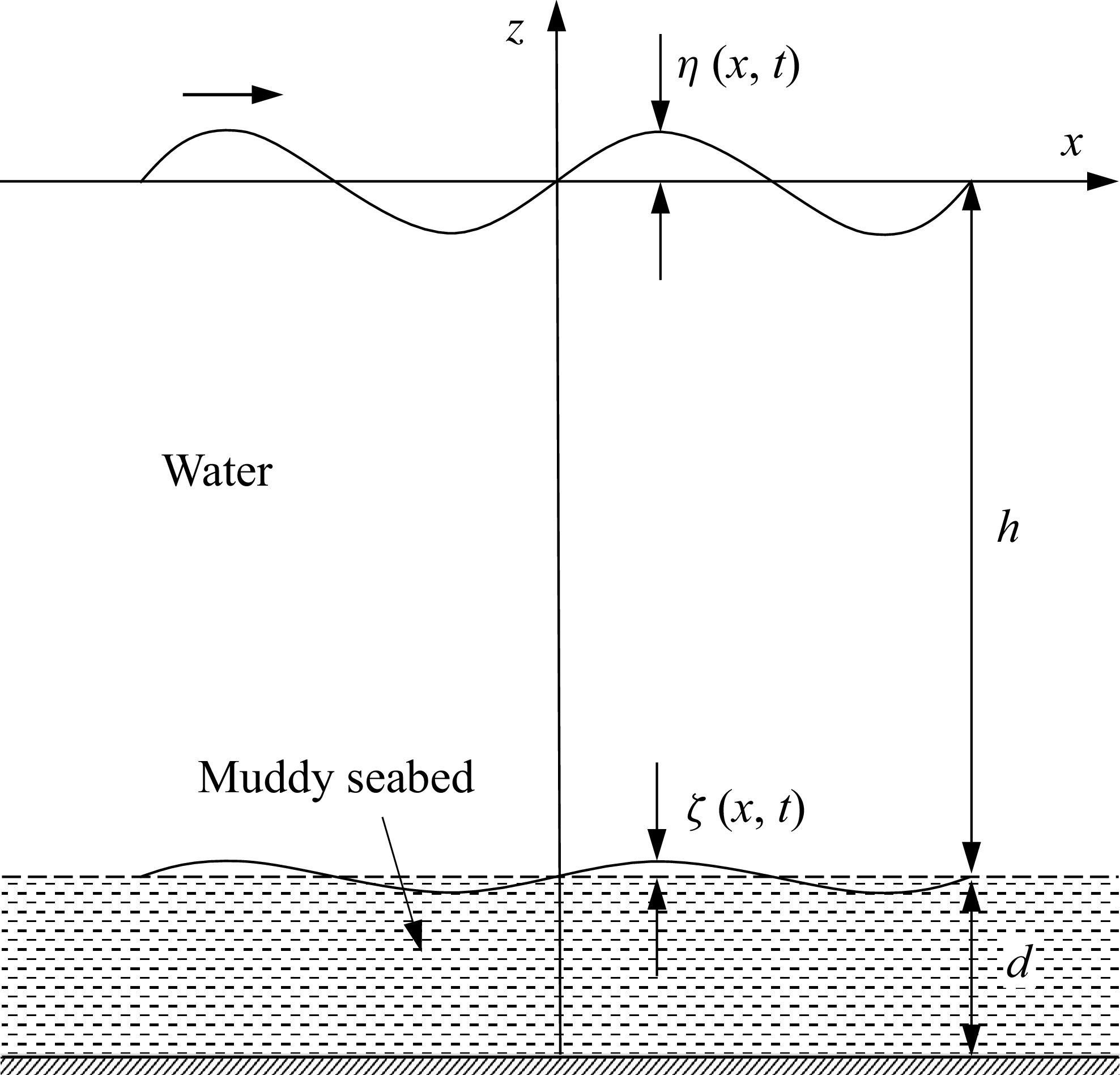
As shown in figure 1, we consider a train of water waves with surface displacement, $\eta ^\prime (x^\prime ,t^\prime )$ , characteristic amplitude, $A$ , frequency, $\omega$ , and wavenumber, $k^\prime$ , propagating in a constant water depth, $h^\prime$ , over a layer of mud with a constant thickness, $d$ . The mud is modelled as a poro-viscoelastic medium, with effective dynamic viscosity, $\mu$ , permeability, $k_s$ , shear modulus, $G$ , and porosity, $n$ . Under the wave loading, the water and mud interface oscillates with a displacement, $\zeta ^\prime$ , and characteristic amplitude, $b$ . The Cartesian coordinates ( $x^\prime$ , $z^\prime$ ) are used on the vertical plane, originating at the still water level. In the analysis, the following normalisations are introduced:

(2.1) \begin{align} \left .\begin{array}{l} \displaystyle x=\frac {\omega ^2}{g}x^\prime ,\quad z=\frac {\omega ^2}{g}{z^\prime },\quad k=\frac {g}{\omega ^2}{k^\prime },\quad t=\omega {t^\prime },\quad \eta =\frac {\eta ^\prime }{A},\\ \displaystyle p=\frac {1}{\rho {gA}}p^\prime , \quad (u,w)=\frac {1}{A\omega }(u^\prime ,w^\prime ),\quad {\varPhi }=\frac {\omega }{gA}{\varPhi }^\prime , \end{array}\right \} \end{align}

for the wave motion, and

(2.2) \begin{align} \left .\begin{array}{l} \displaystyle x=\frac {\omega ^2}{g}x^\prime ,\qquad Z=\frac {z^\prime +h^\prime +d}{d}, \qquad \zeta =\frac {\zeta ^\prime }{\epsilon {A}},\qquad t=\omega {t^\prime },\\[9pt]\displaystyle U=\frac {U^\prime }{A\omega },\quad \mathscr{U}=\frac {\mathscr{U}^{\kern1.5pt \prime} }{A\omega },\quad \displaystyle W=\frac {A}{d}\frac {W^\prime }{\epsilon {A}\omega },\quad \displaystyle \mathscr{W}=\frac {A}{d}\frac {\mathscr{W}^{\kern2.5pt \prime} }{\epsilon {A}\omega },\quad P=\frac {1}{\rho {gA}}P^\prime ,\\[9pt]\displaystyle \boldsymbol{\tilde \tau }_{\textit{ij}}=\frac {d}{\mu _w A\omega }\boldsymbol{\tilde \tau }_{\textit{ij}}^\prime ,\quad \boldsymbol{\tau }_{\textit{ij}}=\frac {d}{\mu A\omega }\boldsymbol{\tau }_{\textit{ij}}^\prime ,\quad {\boldsymbol{\tilde \varepsilon }_{\textit{ij}}}=\frac {d}{A\omega }{{\boldsymbol{\tilde \varepsilon }}_{\textit{ij}}^\prime },\quad {\boldsymbol{\varepsilon }_{\textit{ij}}}=\frac {d}{A\omega }{{\boldsymbol \varepsilon }_{\textit{ij}}^\prime }, \end{array}\right \} \end{align}

for the muddy flow, where $\rho$ is the density of water, $g$ denotes the acceleration of gravity, $k$ indicates the wavenumber, $p$ represents the dynamic water pressure, $\varPhi$ is the velocity potential in the water layer, $P$ indicates the dynamic pressure inside the mud, $\boldsymbol{U}=(U,W)$ and $\boldsymbol{\mathscr{U}}=(\mathscr{U},\mathscr{W}\kern2.5pt)$ denote the dimensionless velocity vectors of the water and mud skeleton in the $x$ direction and $z$ direction, respectively, $\mu$ represents the characteristic dynamic viscosity of the mud, $\boldsymbol{\tilde \tau }_{\textit{ij}}$ and $\boldsymbol \tau _{\textit{ij}}$ are the viscous stresses of the pore fluid and the viscoelastic stresses of the soil skeleton, respectively, $\boldsymbol{\tilde \varepsilon }_{\textit{ij}}$ and $\boldsymbol \varepsilon _{\textit{ij}}$ denote the strain tensors of the pore fluid and soil skeleton, respectively, and

(2.3) \begin{align} \epsilon =\frac {\omega ^2{A}}{g} \end{align}

measures the wave slope, which is typically small. In this study, the superscript prime indicates that the variable is dimensional and the tension is considered positive for the analysis.

Figure 1.

Sketch of water waves propagating over a muddy seabed.

2.1. Governing equations for the wave motion and mud dynamics

For coastal water waves, the phase speed is significantly lower than that of the compressional wave in the water column (Abdolali et al. Reference Abdolali, Kirby and Bellotti2015). Thus, it is assumed that the upper layer of the water is incompressible. Employing (2.1), the dimensionless Navier–Stokes equations for wave motion can be written as (Wen & Liu Reference Wen and Liu1995b )

(2.4) \begin{align} \frac {\partial {u}}{\partial {x}}+\frac {\partial {w}}{\partial {z}}&=0, \end{align}

(2.5) \begin{align} \frac {\partial {u}}{\partial {t}}+\epsilon \left ({u}\frac {\partial {u}}{\partial {x}}+{w}\frac {\partial {u}}{\partial {z}}\right )&=-\frac {\partial {p}}{\partial {x}}+\frac {\delta _w^2}{2}\left (\frac {\partial ^2{u}}{\partial {x^2}}+\frac {\partial ^2u}{\partial {z^2}}\right )\!, \end{align}

(2.6) \begin{align} \frac {\partial {w}}{\partial {t}}+\epsilon \left ({u}\frac {\partial {w}}{\partial {x}}+{w}\frac {\partial {w}}{\partial {z}}\right )&=-\frac {\partial {p}}{\partial {z}}+\frac {\delta _w^2}{2}\left (\frac {\partial ^2{w}}{\partial {x^2}}+\frac {\partial ^2w}{\partial {z^2}}\right )\!, \end{align}

where $\delta _w$ is the normalised thickness of the bottom boundary layer of the water column, i.e.

(2.7) \begin{align} \delta _w=\frac {\omega ^2}{g}\sqrt {\frac {2\mu _w}{\rho \omega }}, \end{align}

with $\mu _w$ denoting the dynamic viscosity of water. For water waves in the coastal region, $\delta _w$ is also a small parameter (Liu & Chan Reference Liu and Chan2007a ). Therefore, the flow in the water is essentially irrotational except in the boundary layer adjacent to the free surface and the bottom of the water column. In the core region of the water column, the governing equation of wave motion can be written as (Mei et al. Reference Mei, Krotov, Huang and Huhe2010)

(2.8) \begin{align} \frac {\partial ^2{\varPhi }}{\partial {x^2}}+\frac {\partial ^2{\varPhi }}{\partial {z^2}}=0. \end{align}

The dynamic water pressure is related to the Bernoulli equation:

(2.9) \begin{align} p+\frac {\partial \varPhi }{\partial {t}}+\frac {\epsilon }{2}\left [\left (\frac {\partial \varPhi }{\partial {x}}\right )^2+\left (\frac {\partial \varPhi }{\partial {z}}\right )^2\right ]=0. \end{align}

Previous studies on wave propagation over muddy seabeds have predominantly employed single-phase medium models to characterise the dynamic response of the seabed (Dalrymple & Liu Reference Dalrymple and Liu1978; Macpherson Reference Macpherson1980; Ng Reference Ng2000; Ng & Zhang Reference Ng and Zhang2007; Mei et al. Reference Mei, Krotov, Huang and Huhe2010; Garnier et al. Reference Garnier, Huang and Mei2013). However, such models inherently neglect the dynamic coupling between the pore fluid and mud skeleton (Yamamoto et al. Reference Yamamoto, Koning, Sellmeijer and Hijum1978; Sumer Reference Sumer2014b ). To address this knowledge gap, this study adopts the general two-phase poro-viscoelastic theory to formulate the governing equations for seabed soil motion. Within the muddy seabed, the continuity equation can be expressed as (Tong & Liu Reference Tong and Liu2022)

(2.10) \begin{align} n\frac {\partial }{\partial {x}}(U-\mathscr{U} \kern1.5pt )+n\frac {\partial }{\partial {Z}}(W-\mathscr{W} \kern2.5pt )+\frac {\partial \mathscr{U}}{\partial {x}}+\frac {\partial \mathscr{W}}{\partial {Z}}=-nM_a^2\frac {\partial {P}}{\partial {t}}, \end{align}

in which $M_a$ represents the Mach number, being defined as the ratio of the characteristic phase velocity of the water wave to the velocity of the compressible wave through the pore fluid,

(2.11) \begin{align} M_a=\sqrt {\frac {\rho }{K}}\frac {g}{\omega }, \end{align}

with $K$ indicating the apparent bulk modulus of elasticity of the pore fluid. As suggested by Verruit (Reference Verruit1969), $K$ depends on the degree of saturation $S_r$ and is given by

(2.12) \begin{align} \frac {1}{K}=\frac {1}{K_w}+\frac {1-S_r}{p^\prime _a}, \end{align}

where $K_w$ is the bulk modulus of elasticity of pure water and $p_a^\prime$ indicates the absolute pore water pressure. For analysis herein, $K_w=2.3\times {10^9}\,\textrm {Pa}$ is used (Liu et al. Reference Liu, Park and Lara2007). Equation (2.10) shows that the motions of the pore fluid and the mud skeleton are affected by the compressibility of the pore fluid with the magnitude of this influence determined by the value of $M_a$ . For an incompressible muddy seabed, $M_a=0$ .

The dimensionless momentum equations for the pore fluid are given by (Ouriemi, Aussilious & Guazzelli Reference Ouriemi, Aussilious and Guazzelli2009; Baumgarten & Kamrin Reference Baumgarten and Kamrin2019b )

(2.13) \begin{align} n\left (\frac {\partial {U}}{\partial {t}}+\epsilon {\boldsymbol{{U}}\boldsymbol{\cdot }\boldsymbol{\nabla }{{U}}}\right )&=-n\frac {\partial {P}}{\partial {x}}+\frac {1}{Re}\frac {A}{d}\left (\epsilon \frac {d}{A}\frac {\partial \tilde \tau _{xx}}{\partial {x}}+\frac {\partial \tilde \tau _{zx}}{\partial {Z}}\right )-\frac {n^2}{D_a}(U-\mathscr{U} \kern1.5pt ), \end{align}

(2.14) \begin{align} n\left (\epsilon \frac {d}{A}\right )^2\left (\frac {\partial {W}}{\partial {t}}+\epsilon {\boldsymbol{U}\boldsymbol{\cdot }\boldsymbol{\nabla }{W}}\right )&=-n\frac {\partial {P}}{\partial {Z}}+\frac {\epsilon }{Re}\left (\epsilon \frac {d}{A}\frac {\partial \tilde \tau _{xz}}{\partial {x}}+\frac {\partial \tilde \tau _{zz}}{\partial {Z}}\right )\nonumber\\&\quad-\left (\epsilon \frac {d}{A}\right )^2\frac {n^2}{D_a}(W-\mathscr{W}\kern2.5pt )\!. \end{align}

in which $D_a$ is the Darcy number, which characterises the magnitude of the drainage flow within the muddy seabed and is defined as

(2.15) \begin{align} {D_a}=\frac {\rho {k_s}\omega }{\mu _\omega }. \end{align}

The dimensionless momentum equations for the skeleton frame of the mud read (Mei & Foda Reference Mei and Foda1981; Baumgarten & Kamrin Reference Baumgarten and Kamrin2019b )

(2.16) \begin{align} (1-n)\gamma \left (\frac {\partial {\mathscr{U}}}{\partial {t}}+\epsilon {\boldsymbol{\mathscr{U}}\boldsymbol{\cdot }\boldsymbol{\nabla }{\mathscr{U}}}\right )&=-(1-n)\frac {\partial {P}}{\partial {x}}+\frac {1}{Re}\frac {A}{d}\left (\epsilon \frac {d}{A}\frac {\partial \tau _{xx}}{\partial {x}}+\frac {\partial \tau _{zx}}{\partial {Z}}\right )\nonumber\\&\quad +\frac {n^2}{D_a}(U-{\mathscr{U}}\kern1.5pt ), \end{align}

(2.17) \begin{align} (1-n)\gamma \left (\epsilon \frac {d}{A}\right )^2\left (\frac {\partial {\mathscr{W}}}{\partial {t}}+\epsilon {\boldsymbol{\mathscr{U}}\boldsymbol{\cdot }\boldsymbol{\nabla }{\mathscr{W}}}\right )&=-(1-n)\frac {\partial {P}}{\partial {Z}}+\frac {\epsilon }{Re}\left (\epsilon \frac {d}{A}\frac {\partial \tau _{xz}}{\partial {x}}+\frac {\partial \tau _{zz}}{\partial {Z}}\right ) \nonumber\\&\quad +\frac {n^2}{D_a}\left (\epsilon \frac {d}{A}\right )^2 (W-{\mathscr{W}}\kern2.5pt ), \end{align}

where $\gamma$ is the density ratio of the mud particles $\varrho$ to that of water $\rho$ , and $Re$ , called the Reynolds number, is the ratio between the viscous force and the elastic force, that is,

(2.18) \begin{align} \textit{Re}=\frac {\rho A\omega d}{\mu } \quad{\textrm {and}} \quad \mu =\sqrt {\mu _m^2+\left (\frac {G}{\omega }\right )^2}, \end{align}

where $\mu _m$ denotes the dynamic viscosity of mud due to grain-to-grain friction (Baumgarten & Kamrin Reference Baumgarten and Kamrin2019a ; Zarch et al. Reference Zarch, Zhang, Haeri and He2025).

According to Newton’s constitutive law and Hooke’s law for compressible media, the viscoelastic stresses for the mud skeleton under simple harmonic wave loading can be expressed as (Macpherson Reference Macpherson1980; Batchelor Reference Batchelor2000)

(2.19) \begin{align} {\boldsymbol{\tau }}_{\textit{ij}}=\widetilde {\mu }{\boldsymbol \varepsilon }_{\textit{ij}}+\widehat \mu \delta _{\textit{ij}}\boldsymbol{\nabla }\boldsymbol{\cdot }\boldsymbol{\mathscr{U}}, \end{align}

where $\boldsymbol{\nabla}$ denotes the gradient operator, i.e. $\boldsymbol{\nabla }= (({\partial }/{\partial {x}}),({\partial }/{\partial {Z}}) )$ , $\delta _{\textit{ij}}$ indicates the Kronecker symbol, $\widetilde {\mu }$ and $\widehat {\mu }$ are complex constants, defined as

(2.20) \begin{align} \widetilde {\mu }=\frac {\mu _m}{\mu }+\frac {{\textrm {i}}G}{\mu \omega }={\textrm {e}}^{{ {i}}\theta }, \qquad \widehat \mu ={\textrm {i}}\frac {2\nu }{1-2\nu }\frac {G}{\mu \omega }-\frac {2\mu _m}{3\mu }\quad {\textrm {and}} \quad {\theta }=\arctan \left ({\frac {G}{\mu _m\omega }}\right )\!, \end{align}

with $\nu$ and $\textrm {i}$ denoting Poisson’s ratio and the imaginary unit, respectively. The mud viscosity $\mu _m$ represents the Coulomb damping due to the friction between grains (Yamamoto, Takahashi & Schuckman Reference Yamamoto, Takahashi and Schuckman1983) and $\theta$ is the argument of $\mu$ , which measures the relative importance of elasticity and viscosity, and it varies from $0$ to $\pi /2$ . For viscous-dominated mud, $\theta \rightarrow {0}$ and for elastic-dominated mud, $\theta \rightarrow {\pi /2}$ . The constitutive law, (2.19), is consistent with that developed by Si, Shi & Yu (Reference Si, Shi and Yu2019).

Finally, the dimensionless strain tensor can be expressed as

(2.21) \begin{align} {\boldsymbol{\varepsilon }_{\textit{ij}}}=\left ( \begin{array}{cc} \displaystyle \varepsilon _{xx} &\, \displaystyle \varepsilon _{zx} \\[9pt] \displaystyle \varepsilon _{xz} &\,\displaystyle \varepsilon _{zz} \\[9pt] \end{array} \right )= \left ( \begin{array}{cc} \displaystyle 2\epsilon \frac {d}{A}\frac {\partial \mathscr{U}}{\partial {x}} &\, \displaystyle \frac {\partial \mathscr{U}}{\partial {Z}}+\left (\epsilon \frac {d}{A}\right )^2\frac {\partial \mathscr{W}}{\partial {x}} \\[9pt] \displaystyle \frac {\partial \mathscr{U}}{\partial {Z}}+\left (\epsilon \frac {d}{A}\right )^2\frac {\partial \mathscr{W}}{\partial {x}} &\,\displaystyle 2\epsilon \frac {d}{A}\frac {\partial \mathscr{W}}{\partial {Z}} \\ \end{array} \right )\!. \end{align}

For incompressible mud, $\boldsymbol{\nabla }\boldsymbol{\cdot }\boldsymbol{{\mathscr{U}}}=0$ , and then the constitutive law, (2.19), reduces to the Kelvin-Voigt model used in Macpherson (Reference Macpherson1980) and Garnier et al. (Reference Garnier, Huang and Mei2013).

2.2. Boundary conditions

The free surface is a material surface, thus, the kinematic condition is given by

(2.22) \begin{align} \frac {\partial {\eta }}{\partial {t}}=\frac {\partial \varPhi }{\partial {z}}-\epsilon \frac {\partial {\eta }}{\partial {x}}\frac {\partial \varPhi }{\partial {x}},\qquad {z=\epsilon {\eta }}. \end{align}

Assuming that the atmospheric pressure is uniform zero at the free surface, for the potential flow, the dynamic boundary condition at the free surface can be written as

(2.23) \begin{align} \eta +\frac {\partial \varPhi }{\partial {t}}+\frac {\epsilon }{2}\left [\left (\frac {\partial \varPhi }{\partial {x}}\right )^2+\left (\frac {\partial \varPhi }{\partial {z}}\right )^2\right ]=0,\qquad {z=\epsilon {\eta }}. \end{align}

The two conditions, (2.22) and (2.23), can be combined into one in terms of $\varPhi$ , taking the total derivative of (2.23):

(2.24) \begin{align} \left (\frac {\partial }{\partial {Z}}+\frac {\partial ^2}{\partial {t^2}}\right )\!{\varPhi }+\epsilon \!\left [\frac {\partial }{\partial {t}}+\frac {\epsilon }{2}\left (\frac {\partial \varPhi }{\partial {x}}\frac {\partial }{\partial {x}}+\frac {\partial \varPhi }{\partial {z}}\frac {\partial }{\partial {z}}\right )\right ]\left [\!\left (\frac {\partial \varPhi }{\partial {x}}\right )^2+\left (\frac {\partial \varPhi }{\partial {z}}\right )^2\right ]=0,\!\quad {z=\epsilon {\eta }}. \end{align}

At the water–seabed interface, the kinematic condition is given by

(2.25) \begin{align} \frac {d}{A}\mathscr{W}=\frac {\partial \zeta }{\partial {t}}+\epsilon \mathscr{U}\frac {\partial \zeta }{\partial {x}} ,\qquad {Z=1+\epsilon \frac {A}{d}\zeta } \end{align}

for the muddy seabed, and

(2.26) \begin{align} \frac {\partial \varPhi }{\partial {z}}=\epsilon \frac {\partial \zeta }{\partial {t}}+\epsilon ^2\frac {\partial \varPhi }{\partial {x}}\frac {\partial \zeta }{\partial {x}} ,\qquad z=-h+\epsilon ^2\zeta \end{align}

for water, where $h$ is the normalised depth of the water column. The velocity of the pore fluid and water must be continuous,

(2.27) \begin{align} u=U,\qquad w=\frac {d}{A}\epsilon W,\qquad z=-h+\epsilon ^2\zeta . \end{align}

Since the mud seabed is porous, the pressure will also be continuous at the water–seabed interface, i.e.

(2.28) \begin{align} p=P,\qquad z=-h+\epsilon ^2\zeta . \end{align}

Meanwhile, continuity of the stresses at the water–mud interface requires that

(2.29) \begin{align}& \tilde \tau _{xx}n_x+\tilde {\tau }_{zx}n_z=2\epsilon \frac {d}{A}\frac {\partial {u}}{\partial {x}}n_x+\epsilon \frac {d}{A}\left (\frac {\partial {w}}{\partial {x}}+\frac {\partial {u}}{\partial {z}}\right )n_z,\qquad {z=-h+\epsilon ^2\zeta }, \end{align}

(2.30) \begin{align}& \tilde {\tau }_{xz}n_x+\tilde {\tau }_{zz}n_z=\epsilon \frac {d}{A}\left (\frac {\partial {w}}{\partial {x}}+\frac {\partial {u}}{\partial {z}}\right )n_x+2\epsilon \frac {d}{A}\frac {\partial {w}}{\partial {z}}n_z,\qquad {z=-h+\epsilon ^2\zeta } \end{align}

for water, and

(2.31) \begin{align} (\tau _{x0}+\tau _{xx})n_x+\tau _{zx}n_z&=0,\qquad {Z=1+\epsilon \frac {A}{d}\zeta }, \end{align}

(2.32) \begin{align} \tau _{xz}n_x+ (\tau _{z0}+\tau _{zz})n_z&=0,\qquad {Z=1+\epsilon \frac {A}{d}\zeta } \end{align}

for the soil skeleton, where $n_x$ and $n_z$ are the horizontal and vertical components of the unit normal vector of the water–mud interface:

(2.33) \begin{align} n_x=\frac {\epsilon ^2\displaystyle {\frac {d}{A}\frac {\partial \zeta }{\partial {x}}}}{\sqrt {1+\left (\epsilon ^2\displaystyle {\frac {d}{A}\frac {\partial \zeta }{\partial {x}}}\right )^2} }, \quad n_z=\frac {1}{\sqrt {1+\left (\epsilon ^2\displaystyle {\frac {d}{A}\frac {\partial \zeta }{\partial {x}}}\right )^2} }. \end{align}

Clearly, $n_x$ and $n_z$ are of the order of magnitude of $O(\epsilon ^2)$ and $O(1)$ , respectively. In (2.31) and (2.32), $\tau _{x0}$ and $\tau _{z0}$ are normal stresses in the hydrostatic state in the $x$ and $z$ directions, respectively. Under the hydrostatic equilibrium condition, the shear stress of the mud skeleton vanishes, and the normal effective stresses are given by (Madsen Reference Madsen1978; Tong & Liu Reference Tong and Liu2022)

(2.34) \begin{align} \tau _{x0}=\frac {\nu }{1-\nu }\frac {d}{A}{\gamma _e}(Z-1), \quad \tau _{z0}=\frac {d}{A}{\gamma _e}(Z-1), \end{align}

where $\gamma _e=(1-n)(\gamma -1)$ is the ratio of the submerged unit weight of mud to the unit weight of water.

Following Tong & Liu (Reference Tong and Liu2022), the bottom of the seabed is assumed to be rigid and impermeable. The horizontal and vertical velocity components of the mud skeleton are equal to zero, and the vertical pressure gradient vanishes:

(2.35) \begin{align} \mathscr{U}=\mathscr{W}=\frac {\partial {P}}{\partial {Z}}=0, \qquad {Z=0}. \end{align}

The boundary conditions indicate that the mud is forced to move passively by the hydrodynamic pressure and the viscous stresses from the surface waves. To solve this coupled boundary value problem, we introduce simplifying assumptions grounded in the characteristic scales of coastal waves and the rheological properties of mud. Subsequently, we apply a multiscale perturbation method to obtain analytical solutions for the flow fields in both the water column and the muddy seabed. The key assumptions and the solution procedure are detailed in the following subsections.

3. Scalings and assumptions

In this study we focus on investigating the wave propagating over a thin mud layer. Therefore, following Liu & Chan (Reference Liu and Chan2007b ), the thickness of the muddy seabed is assumed to be of the same order of magnitude as the wave amplitude, i.e.

(3.1) \begin{align} O\left (\frac {d}{A}\right )\,{\sim }\,O(1). \end{align}

The apparent bulk modulus of elasticity of the pore fluid, $K$ , is sensitive to $S_r$ (Liu et al. Reference Liu, Park and Lara2007). For example, when $S_r$ decreases from 1 to 0.9, $K$ decreases from $2.3\times 10^9$ Pa to $1\times 10^6$ Pa for the mud under a water depth of 10 m. Correspondingly, the velocity of the compressible wave within the pore fluid is close to the phase velocity of the wind waves. Therefore, the Mach number is treated as being of the order of magnitude of $O(1)$ :

(3.2) \begin{align} O\left (M_a\right )\,{\sim }\, O(1). \end{align}

This assumption agrees well with some in situ measurements. For example, Bennett & Faris (Reference Bennett and Faris1979) reports that the saturation degree of the mud in the Mississippi Delta is 0.9, and therefore, $M_a=0.63$ when $h=10\,\textrm {m}$ and $\omega =0.5{\,\textrm {s}}^{-1}$ , and $M_a=1.05$ when $h=10\,\textrm {m}$ and $\omega =0.3{\,\textrm {s}}^{-1}$ . For a highly saturated seabed, $M_a\rightarrow {0}$ , and further simplification is possible.

The shear modulus ranges widely from $O(10^3\,\textrm {Pa})$ for soft seabeds to $O(10^8\,\textrm {Pa})$ for dense seabeds (Yamamoto et al. Reference Yamamoto, Koning, Sellmeijer and Hijum1978; Macpherson Reference Macpherson1980; Liu & Chan Reference Liu and Chan2007b ), and the mud viscosity varies from $O(10\,\textrm {Pa}\boldsymbol{\, }\rm s)$ to $O(10^4\,\textrm {Pa}\boldsymbol{\, }\rm s)$ . Correspondingly, the Reynolds number, $Re$ , varies from $O(10^{-5})$ to $O(10)$ (Wen & Liu Reference Wen and Liu1995a ). For a stiff seabed, $Re$ is small, indicating that the inertia force is less important. For a soft muddy seabed, $Re$ is relatively large. For example, the characteristic mud viscosity in Lianyungang, China is of the order of magnitude of $O(10^3$ Pa s) – $O(10^4$ Pa s) when $n=0.5$ (Mei et al. Reference Mei, Krotov, Huang and Huhe2010; Garnier et al. Reference Garnier, Huang and Mei2013). As a rough estimation, $\textit{Re}=1.0$ when $\mu =10^3$ Pa s, and $\textit{Re}=0.1$ when $\mu =10^4$ Pa s together with $\omega =1.0\,\rm {rad\,s^{-1}}$ and $A=d=1.0\,\textrm {m}$ . Therefore, $Re$ is also assumed to be of the order of magnitude of $O(1)$ , that is,

(3.3) \begin{align} O(Re)\,{\sim }\, O (M_a)\,{\sim }\, O(1). \end{align}

Physically, it means that viscous and elastic effects throughout the mud seabed are treated without the boundary layer approximation.

For the muddy seabed, the Darcy number, $D_a$ , is very small. For example, $k_s$ is of the order of magnitude of $O(10^{-13}\,{{\textrm {m}}^2})$ or even smaller in a silty or clayey seabed (Liu et al. Reference Liu, Park and Lara2007). For approximation, we take $k_s=10^{-13}\,{{\textrm {m}}^2}$ , $\omega =0.5\,\rm {rad\,s^{-1}}$ and $\mu _w=10^{-3}$ Pa s, then $D_a=5\times {10^{-8}}$ . Therefore, the following relation with respect to $D_a$ and $\epsilon$ shall be satisfied:

(3.4) \begin{align} O(D_a)\ll {O(\epsilon ^3)}\ll {O(\epsilon )}\ll {1}. \end{align}

This means that the drainage effects are negligible for the wave-induced mud dynamics.

For waves in the coastal region, the thickness of the bottom boundary layer is usually small and is assumed to be $O(\epsilon )$ (Longguet-Higgins Reference Longguet-Higgins1953; Ng Reference Ng2000), that is,

(3.5) \begin{align} O(\delta _w)\sim {O(\epsilon )}\ll {1}. \end{align}

In estimation, take $\omega =0.5$ – $2\,\rm {rad\,s}^{-1}$ and eddy viscosity $\mu _w=1.0$ Pa s, then $\delta _w=0.16$ – $1.3\times {10}^{-2}$ . Thus, the above assumption is approximately satisfied.

4. Perturbation analysis

Based on (3.1)–(3.5), the dynamics of the flow problem can be presented in the following manner. In the core region of the water column, the flow is irrotational and can be described by potential flow theory. Given that the vertical displacement of the water–seabed interface is small, $O(\epsilon )$ , and the drainage flow is quite weak, $O(D_a)$ , in the leading-order problem, the wave motion does not sense the muddy seabed and so the solution for irrotational motion coincides with the well-known potential flow solution for small-amplitude waves over a solid bottom. However, the dynamic pressure at the water–seabed interface induces a shear flow within the muddy seabed. The horizontal and vertical velocity components of the shear flow are of the order of magnitude of $O(1)$ and $O(\epsilon )$ , respectively. Meanwhile, a leading-order horizontal rotational velocity develops within the bottom boundary layer of the water column to satisfy the continuity of velocity and viscous shear stress across the interface. According to the continuity equation, a vertical velocity component of $O(\delta _w)$ must also arise within this boundary layer. As a result, the irrotational flow in the core region must be corrected at $O(\delta _w)$ . Due to the nonlinear interactions between the velocity components, mass transport occurs within the water column and muddy seabed, which is of the order of magnitude of $O(\epsilon )$ . The rotational horizontal velocity within the free surface boundary layer, $O(\delta _w)$ , is weaker since only the zero shear stress is imposed at the free surface (Mei & Liu Reference Mei and Liu1973), and correspondingly, the vertical rotational velocity inside this boundary layer is $O(\delta _w^2)$ , which has no influence on wave and mud motions, correct to $O(\epsilon )$ , except for introducing a second-order mean Eulerian vorticity outside the boundary layer.

In the dimensionless governing equations and boundary conditions, $\epsilon$ , $D_a$ and $\delta _w$ are three small dimensionless parameters. For small-amplitude progressive waves, it is natural to employ the asymptotic method of perturbations. According to (3.1)−(3.5), $\epsilon$ is chosen as the ordering small parameter. Anticipating that wave damping will become significant only after propagating over a long distance, the following multiple-scale coordinates are introduced in terms of $\epsilon$ ,

(4.1) \begin{align} t,\quad t_1=\epsilon {t},\quad t_2=\epsilon ^2t,{\cdots} ;\qquad x,\quad x_1=\epsilon {x},\quad x_2=\epsilon ^2{x},{\cdots} . \end{align}

The derivatives with respect to $t$ must now be replaced by

(4.2) \begin{align} \frac {\partial }{\partial {t}}=\frac {\partial }{\partial {t}}+\epsilon \frac {\partial }{\partial {t_1}}+\epsilon ^2\frac {\partial }{\partial {t_2}}+{\cdots} , \quad \frac {\partial ^2}{\partial {t}^2}=\frac {\partial ^2}{\partial {t}^2}+2\epsilon \frac {\partial ^2}{\partial {t}\partial {t_1}}+\epsilon ^2\left (\frac {\partial ^2}{\partial {t_1^2}}+\frac {\partial ^2}{\partial {t}\partial {t_2}}\right )+{\cdots} . \end{align}

Similar replacements must be made for derivatives with respect to $x$ , while derivatives with respect to $z$ and $Z$ remain the same.

For slowly varying harmonic waves, the variables, such as $\varPhi$ , $p$ , $P$ , $ (u,w )$ , $ (U,W )$ and $\tau _{\textit{ij}}$ , can be expanded as follows:

(4.3) \begin{align} \mathscr{F}=\frac {1}{2}\big [\mathscr{F}_0+\epsilon \mathscr{F}_1+\epsilon ^2\mathscr{F}_2+{\cdots} \big ]{\rm e}^{{\textrm {i}}(kx-t)}+\textrm {c.c.} \end{align}

Here $(\eta _n,\zeta _n)$ depend only on $(x_1, {\cdots} ; t_1,{\cdots} )$ , $\varPhi _n$ on $(x_1, {\cdots} ; z; t_1,{\cdots} )$ in the water column and $(U_n,W_n,u_n,w_n)$ on $(x_1, {\cdots} ; Z; t_1,{\cdots} )$ in the muddy seabed, `c.c.’ denotes the conjugate complex of the preceding terms. In addition, there is an additional horizontal length scale due to the motion of the muddy seabed, $O(1/k\epsilon )$ , and therefore, the wavenumber is also expanded in power of $\epsilon$ :

(4.4) \begin{align} k=k_0+\epsilon {k}_1+\epsilon ^2{k}_2+{\cdots} . \end{align}

Since the free surface oscillates with displacement of $\epsilon \eta$ , the general variable, $\mathscr{F}$ , can be expanded in terms of the Taylor series, i.e.

(4.5) \begin{align} {\mathscr{F}}({x,\epsilon \eta },t)={\mathscr{F}}(x,0,t)+\epsilon \eta \left .\frac {\partial {{\mathscr{F}}}}{\partial {z}}\right |_{z=0}+\epsilon ^2\eta ^2\frac {1}{2}\left .\frac {\partial ^2{{\mathscr{F}}}}{\partial {z}^2}\right |_{z=0}+{\cdots} . \end{align}

Similarly, at the water–mud interface, $\mathscr{F}$ can be expanded as

(4.6) \begin{align} {\mathscr{F}}(x,-h+{\epsilon ^2\zeta },t)={\mathscr{F}}(x,-h,t)+\epsilon ^2\zeta \left .\frac {\partial {{\mathscr{F}}}}{\partial {z}}\right |_{z=-h}+{\cdots} \end{align}

for the variables within the water column, and

(4.7) \begin{align} \mathscr{F}(x,1+\epsilon \frac {A}{d}\zeta ,t)=\mathscr{F}(x,1,t)+\epsilon \frac {A}{d}\zeta \left .\frac {\partial {\mathscr{F}}}{\partial {Z}}\right |_{Z=1}+\frac {1}{2}\left (\epsilon \frac {A}{d}\zeta \right )^2\left .\frac {\partial {\mathscr{F}}}{\partial {Z}}\right |_{Z=1}+{\cdots} \end{align}

for the variables within the muddy seabed.

Substituting the expansions (4.1)–(4.6) into the dimensionless governing equations and boundary conditions, a series of perturbation equations can be obtained after separating the orders. In this study the leading-order and second-order boundary value problems are solved and investigated in detail.

5. Leading-order boundary value problems for water and mud motions

Based on the assumptions given in § 3, the leading-order boundary value problems for water and mud motions are summarised and solved in this section, respectively.

5.1. Inviscid flow within the water column

At the leading order, the oscillation of the water–seabed interface and the nonlinear terms have no influence on the wave motion. Correspondingly, the boundary value problem for the wave motion can be summarised as

(5.1) \begin{align} -k_0^2{\varPhi }_0+\frac {{ {d}}^2{\varPhi }_0}{{\textrm {d}}{z^2}}=0, \quad \, {-h\,\lt \,z\,\lt \,0}, \end{align}

with

(5.2) \begin{align}& \frac {\partial {\varPhi }_0}{\partial {z}}-{{\varPhi }}_0=0, \quad {z=0}, \end{align}

(5.3) \begin{align}&\quad \frac {\partial {\varPhi }_0}{\partial {z}}=0, \quad {z=0}. \end{align}

(5.4) \begin{align}&\quad \eta _0={\textrm {i}}{\varPhi }_0, \quad {z=0}. \end{align}

The leading-order solution for the velocity potential ${\varPhi }_0$ can be readily obtained by solving the two-point boundary value problem (5.1)–(5.3), which can be written as

(5.5) \begin{align} {\varPhi }_0=-{\textrm {i}}\hat {A}\frac {\cosh {Q}}{\cosh {q}}, \end{align}

where

(5.6) \begin{align} Q\,{\equiv }\,k_0(z+h),\quad \, q\,{\equiv }\,k_0h. \end{align}

Based on (5.4), the free surface elevation can be written as

(5.7) \begin{align} \eta _0=\hat {A}, \end{align}

with the dispersion relationship of

(5.8) \begin{align} k_0\tanh {k_0h}=1. \end{align}

It should be remarked that $\hat {A}$ depends on the slow coordinates and is yet unknown. For later use, the potential velocity components of water are calculated by differentiating the velocity potential with respect to $x$ and $z$ , respectively, that is,

(5.9) \begin{align}&\,\,\, \widehat {u}_0=\frac {\partial {\varPhi }_0}{\partial {x}}=k_0\hat {A}\frac {\cosh {Q}}{\cosh {q}}=\hat {A}\frac {\cosh {Q}}{\sinh {q}}, \end{align}

(5.10) \begin{align}& \widehat {w}_0=\frac {\partial {\varPhi }_0}{\partial {z}}=-{\textrm {i}}k_0\hat {A}\frac {\sinh {Q}}{\cosh {q}}=-{\textrm {i}}\hat {A}\frac {\sinh {Q}}{\sinh {q}}. \end{align}

According to (2.9), the following leading-order dynamic pressure can be obtained:

(5.11) \begin{align} p_0={\textrm {i}}{\varPhi }_0=\hat {A}\frac {\cosh {Q}}{\cosh {q}}. \end{align}

This has a finite value along the water bottom, $z=-h$ ,

(5.12) \begin{align} p_b=\left .p_0\right |_{z=-h}=\frac {\hat {A}}{\cosh {q}}, \end{align}

and, in turn, it generates muddy flow within the seabed.

5.2. Viscid flows within the Stokes boundary layer and muddy seabed

Since the Stokes boundary layer in water is thin, a stretched coordinate $\xi$ is introduced as

(5.13) \begin{align} \xi =\frac {z+h}{\delta _w}. \end{align}

Hence, the continuity equation for the rotational velocity components can be written as

(5.14) \begin{align} {\textrm {i}}k_0{{u}_0^r}+\frac {1}{\delta _w}\frac {\partial {w}_0^r}{\partial {\xi }}=0,\qquad 0\lt \xi \lt \infty . \end{align}

According to (2.5), the governing equation of the rotational component of the horizontal velocity can be expressed as

(5.15) \begin{align} \frac {\partial ^2u_0^r}{\partial {\xi ^2}}+2{\textrm {i}}{{u_0^r}}=0,\qquad 0\lt \xi \lt \infty . \end{align}

Based on (2.13), (2.14), (3.4) and (3.5), it is known that

(5.16) \begin{align}& U_0=\mathscr{U}_0,\qquad 0\lt Z\lt 1, \end{align}

(5.17) \begin{align}& W_0=\mathscr{W}_0,\qquad 0\lt Z\lt 1, \end{align}

correct to $O(Da)$ , indicating that the pore fluid moves with the mud skeleton as a block in the leading-order boundary value problem. Therefore, the continuity equation of the muddy flow can be written as

(5.18) \begin{align} {\textrm {i}}k_0{\mathscr{U}}_0+\frac {\partial {\mathscr{W}}_0}{\partial {Z}}={\textrm {i}}nM_a^2P_0,\qquad 0\lt Z\lt 1. \end{align}

Since the pore fluid moves with the mud skeleton as a block, the viscosity of the pore fluid can be absorbed into that of the mud skeleton. Thus, hereinafter $\mu _m$ stands for the total viscosity of the mud block. Combining the momentum equations for the mud skeleton with that for the pore fluid, the leading-order momentum equations for the mud block are obtained to be

(5.19) \begin{align}& -{\textrm {i}}\gamma _m{{\mathscr{U}}_0}=-{\textrm {i}}k_0{P_0}+\frac {\widetilde {\mu }}{Re}\frac {A}{d}\frac {{ {d}}^2{\mathscr{U}}_0}{{\textrm {d}}{Z}^2},\qquad 0\lt Z\lt 1, \end{align}

(5.20) \begin{align}&\qquad\qquad\quad \frac {\partial {P_0}}{\partial {Z}}=0,\qquad 0\lt Z\lt 1, \end{align}

where $\gamma_m$ is the density ratio of the mud block to water, namely $\gamma_m=(1-n)\gamma+n$ . Based on (5.20), it is known that the dynamic pore pressure is uniform in the $Z$ direction,

(5.21) \begin{align} P_0=p_b=\frac {\hat {A}}{\cosh {q}}. \end{align}

Thus, the boundary value problem for the horizontal velocity of the mud can be expressed as

(5.22) \begin{align} \frac {{ {d}}^2{\mathscr{U}}_0}{{\textrm {d}}{Z}^2}-\sigma ^2{\mathscr{U}_0}=-\frac {\sigma ^2}{\gamma _m}\frac {\hat {A}}{\sinh {q}},\qquad 0\lt Z\lt 1, \end{align}

where

(5.23) \begin{align} \sigma = \sqrt {-{\textrm {i}}\gamma _m\frac {Re}{\widetilde {\mu }}\frac {d}{A}}=\sqrt {2}\widehat {d}{\textrm {e}}^{-{ \textrm{i}}\left (\tfrac {\theta }{2}+\tfrac {\pi }{4}\right )},\quad \widehat {d}=\frac {d}{\delta _m^\prime } \; {\textrm {and}}\;\, \delta _m^\prime =\sqrt {\frac {2\mu }{\rho _m\omega }}, \end{align}

with $\rho _m$ and $\delta _m^\prime$ denoting the density of the mud and the thickness of the Stokes boundary layer of the muddy seabed, respectively.

Since the flow in the core region is inviscid, the rotational velocity vanishes beyond the Stokes boundary layer ( $\xi \rightarrow \infty$ ). At the water–seabed interface, the velocity and shear stress are continuous. At the bottom of the seabed, the horizontal velocity component is equal to zero. Therefore, the following conditions are satisfied for viscid flows within the Stokes boundary layer and muddy seabed:

(5.24) \begin{align}&\qquad\qquad \frac {\partial {u_0^r}}{\partial {\xi }}=0, \qquad \xi \rightarrow \infty , \end{align}

(5.25) \begin{align}&\quad {\mathscr{U}}_0=\frac {\hat {A}}{\sinh {q}}+u_0^r,\qquad \xi =0\;({\textrm {or}}\; Z=1), \end{align}

(5.26) \begin{align}& \mu {\textrm {e}^{\textrm {i}\theta }}\frac {\partial {{\mathscr{U}}_0}}{\partial {Z}}=\epsilon \frac {d}{A}\frac {\mu _w}{\delta _w}\frac {\partial {u_0^r}}{\partial {\xi }},\qquad \xi =0\; ({\textrm {or}}\; Z=1), \end{align}

(5.27) \begin{align}&\qquad\qquad\quad {\mathscr{U}_0}=0,\qquad Z=0. \end{align}

The boundary value problem (5.15), (5.22) and (5.24)–(5.27) can be explicitly solved, and the solution can be written as

(5.28) \begin{align}&\qquad\qquad\quad u_0^r=D\frac {\hat {A}}{\sinh {q}}{\textrm {e}}^{-(1-{ \textrm{i}})\xi }, \end{align}

(5.29) \begin{align}& \mathscr{U}_0=\frac {1}{\gamma _m}\frac {\hat {A}}{\sinh {q}}\left (1-\cosh {(\sigma \kern-1pt Z)}+F\sinh {(\sigma \kern-1pt Z)}\right )\!, \end{align}

where

(5.30) \begin{align}& D= \frac {-\beta -\beta (\gamma _m-1)\cosh {\sigma }}{\gamma _m\beta \cosh {\sigma }+\sinh {\sigma }}, \end{align}

(5.31) \begin{align}& F=\frac {\gamma _m-1+\cosh {\sigma }+\beta \gamma _m \sinh {\sigma }}{\gamma _m\beta \cosh {\sigma } +\sinh {\sigma }}. \\[12pt] \nonumber \end{align}

In (5.30) and (5.31), $\beta =\delta _m^\prime {\textrm {e}}^{{{ \textrm{i}}( {\theta }/{2}})}/\delta _w^{\prime }$ measures the ratio of the Stokes boundary layer thickness. Since mud is typically more viscous than water, $\beta$ is commonly much larger than unity (Liu & Chan Reference Liu and Chan2007a ; Garnier et al. Reference Garnier, Huang and Mei2013). If mud is pure viscous, the solution of $u_0^r$ and $\mathscr{U}_0$ , (5.28) and (5.29), agrees with the results of Ng (Reference Ng2000), and if the viscosity of water is ignored, $\beta \rightarrow \infty$ , then (5.29) reduces to the results of Mei et al. (Reference Mei, Krotov, Huang and Huhe2010).

At the bottom of the seabed, the leading-order vertical velocity component of mud vanishes. Thus, substituting (5.29) and (5.21) into (5.18) and integrating with respect to $Z$ from 0 to $Z$ yields the vertical velocity component of mud flow:

(5.32) \begin{align} \mathscr{W}_0={\textrm {i}}nM_a^2\frac {\hat {A}}{\cosh {q}}Z-{\textrm {i}}\frac {k_0}{\gamma _m}\frac {\hat {A}}{\sinh {q}}\left [Z-\frac {\sinh {(\sigma \kern-1pt Z)}}{\sigma }+F\frac {\cosh {(\sigma \kern-1pt Z)}-1}{\sigma }\right ]. \end{align}

The first term on the right-hand side of (5.32) signifies the effect of compressibility on mud motion. For an incompressible muddy seabed, $M_a=0$ and $\mathscr{W}_0$ reduces to the result of Ng & Zhang (Reference Ng and Zhang2007). Inside the bottom boundary layer, the total horizontal velocity component, $u_{0}$ , can be written as

(5.33) \begin{align} u_0=\widehat {u}_0+u_0^r=\big [1+D{\textrm {e}}^{-(1-{\textrm{i}})\xi }\big ]\frac {\hat {A}}{\sinh {q}}. \end{align}

If $d=0$ then $\sigma =0$ , therefore, $\cosh {\sigma }=1$ and $\sinh {\sigma }=0$ . Consequently, $D=-1$ and (5.33) reduces to the results of Mei et al. (Reference Mei, Stiassnie and Yue2005). At the water–seabed interface, the vertical velocity component of mud and water should also be continuous, and $w_0$ vanishes. Thus, based on (5.14), the vertical rotational velocity component can be found by integration with respect to $\xi$ , i.e.

(5.34) \begin{align} {w}_0^r=\epsilon \frac {d}{A}\left ({\textrm {i}}nM_a^2\frac {\hat {A}}{\cosh {q}}-{\textrm {i}}\frac {k_0}{\gamma _m}\frac {\hat {A}}{\sinh {q}}\mathscr{G}(\sigma ,\beta )\right )+{\textrm {i}}\delta _wD\frac {k_0\hat {A}}{\sinh {q}}\frac {{\textrm {e}^{-(1-{ \textrm{i})\xi }}-1}}{1-{\textrm {i}}}, \end{align}

where

(5.35) \begin{align} \mathscr{G}(\sigma ,\beta )=1-\frac {\sinh {\sigma }}{\sigma }+F\frac {\cosh {\sigma }-1}{\sigma }. \end{align}

Accordingly, the total vertical velocity component, $w_0$ , within the bottom boundary layer is given by

(5.36) \begin{align} {w}_0=\epsilon \frac {d}{A}\mathscr{W}_s- \textrm {i}\delta _w\frac {k_0\hat {A}}{\sinh {q}}\left [\xi -D\frac {\textrm {e}^{-(1-{\textrm{i})\xi }}-1}{1-\textrm {i}}\right ]\!, \end{align}

where $\mathscr{W}_s$ is the vertical velocity component of the mud at the water–seabed interface, i.e.

(5.37) \begin{align} \mathscr{W}_s= {\textrm {i}}\frac {k_0\hat {A}}{\sinh {q}} \left ({nM_a^2}\tanh ^2{q}-\frac {\mathscr{G}(\sigma ,\beta )}{\gamma _m}\right )\!. \end{align}

Equation (5.36) demonstrates that the vertical velocity component is of order $O(\epsilon )$ , which is one order of magnitude smaller than the horizontal velocity component. Finally, the vertical displacement of the water–seabed interface, $\zeta _0$ , is calculated from (2.25) at the leading order:

(5.38) \begin{align} \zeta _0=\textrm {i}\frac {d}{A}\mathscr{W}_s=\frac {d}{A}\frac {k_0\hat {A}}{\sinh {q}}\left (\frac {\mathscr{G}(\sigma ,\beta )}{\gamma _m} -nM_a^2\tanh ^2{q}\right )\!. \end{align}

We reiterate that $\hat {A}$ , which depends on the slow coordinates, is still unknown.

The leading-order solutions above reveal that, although seabed compressibility exerts no influence on the leading-order horizontal velocity components in either the water column or the muddy seabed, it does induce measurable deviations in the vertical velocity component within both the Stokes boundary layer and the muddy seabed, relative to predictions from single-phase incompressible models. Crucially, this compressibility-induced deviation cannot be compensated by adjusting the shear modulus or viscosity of the mud in single-phase incompressible models.

6. The second-order boundary value problems

6.1. Evolution of the wave envelope

The governing equation of the first-order velocity potential can be expressed as

(6.1) \begin{align} \frac {\partial ^2{\varPhi }_1}{\partial {z^2}}-k_0^2{\varPhi }_1=-2{\textrm {i}}k_0\frac {\partial {\varPhi }_0}{\partial {x_1}}=-2k_0\frac {\cosh {Q}}{\cosh {q}}\frac {\partial \hat {A}}{\partial {x_1}}, \end{align}

and the boundary conditions are given by

(6.2) \begin{align} \frac {\partial {\varPhi }_1}{\partial {z}}-{\varPhi }_1&=2{\textrm {i}}\frac {\partial {\varPhi }_0}{\partial {t_1}}=2\frac {\partial \hat {A}}{\partial {t_1}},\qquad z=0, \end{align}

(6.3) \begin{align} \frac {\partial {\varPhi }_1}{\partial {z}}&=-{\textrm {i}}\zeta _0,\qquad z=-h. \end{align}

The boundary value problem (6.1)–(6.3) is non-homogeneous. Since the homogeneous version of the boundary value problem has ${\varPhi }_0$ as a non-trivial solution, the non-homogeneous problem must satisfy a solvability condition, which follows by applying Green’s theorem to ${\varPhi }_0$ and ${\varPhi }_1$ (Mei et al. Reference Mei, Stiassnie and Yue2005):

(6.4) \begin{align} \int _{-h}^0\left [{\varPhi }_0\left (\frac {\partial ^2{\varPhi }_1}{\partial {z^2}}-k_0^2{\varPhi }_1\right )+{\varPhi }_1\left (\frac {\partial ^2{\varPhi }_0}{\partial {z^2}}-k_0^2{\varPhi }_0\right )\right ]{\rm d}z=\left .\left ({\varPhi }_0\frac {\partial {\varPhi }_1}{\partial {z}}-{\varPhi }_1\frac {\partial {\varPhi }_0}{\partial {z}}\right )\right |_{z=-h}^{z=0}. \end{align}

Substituting (5.1)–(5.3) and (6.1)–(6.3) into (6.4) yields the following evolution equation of the free surface elevation $\hat {A}$ :

(6.5) \begin{align} \frac {\partial \hat {A}}{\partial {t_1}}+C_g\frac {\partial \hat {A}}{\partial {x_1}}={\textrm {i}}k_1C_g{\hat {A}}. \end{align}

Here $C_g$ is the dimensionless wave group velocity,

(6.6) \begin{align} C_g=\frac {1}{2k_0}\left (1+\frac {2q}{\sinh {2q}}\right )\!, \end{align}

and the first-order wavenumber $k_1$ is given by

(6.7) \begin{align} k_1=-\frac {1}{\gamma _m}\frac {d}{A}\frac {2k_0^2}{\sinh {2q}+2q}\left ( \mathscr{G}(\sigma ,\beta )-nM_a^2{\gamma _m}\tanh ^2{q}\right )\!. \end{align}

The right-hand side of (6.5) signifies the effect of the mud motion on the evolution of the envelope of the leading-order wave. For simple harmonic waves, the wave envelope is independent of $t_1$ , and therefore, the wave amplitude $\hat {A}$ can be found as

(6.8) \begin{align} \hat {A}=A_0{\textrm {e}}^{{\textrm{i}}k_1x_1}=A_0{\textrm {e}}^{-\epsilon k_1^ix}{\textrm {e}}^{{\textrm{i}}\epsilon k_1^rx},\qquad {x_1\gt 0}, \end{align}

where $A_0$ is the normalised wave amplitude at $x_1=0$ that can be taken to be unity, $k_1^r$ and $k_1^i$ are the real and imaginary parts of $k_1$ , respectively. According to (6.8), it is known that due to the flow within the muddy seabed, the surface wave damps slowly at a rate of $\epsilon k_1^i$ and with a phase shift of $\epsilon k_1^r$ .

Substituting (6.8) into (6.1) and (6.2), now the boundary value problem (6.1)–(6.3) can be solved straightforwardly, and the solution can be written as

(6.9) \begin{align}& {\varPhi }_1=2{\textrm {i}}k_1C_g\hat {A}\sinh {q}\sinh {Q}-\frac {1}{k_0}\frac {Q\sinh {Q}}{\cosh {q}}\frac {\partial {\hat {A}}}{\partial {x_1}}, \end{align}

(6.10) \begin{align}& P_1=- \!\left (\!\frac {\partial {\varPhi }_0}{\partial {t_1}}+\frac {\partial {\varPhi }_1}{\partial {t}}\!\right )=\frac {\textrm {i}}{\cosh {q}}\left (\!\frac {\partial \hat {A}}{\partial {t_1}}{\cosh {Q}}-\frac {{Q}}{k_0}\frac {\partial {\hat {A}}}{\partial {x_1}}\sinh {Q}\!\right )-2k_1C_g\hat {A}\sinh {q}\sinh {Q}, \end{align}

(6.11) \begin{align}& \eta _1=- \!\left .\left (\frac {\partial {\varPhi }_0}{\partial {t_1}}+\frac {\partial {\varPhi }_1}{\partial {t}}\right )\right |_{z=0}={\textrm {i}}\left (\frac {\partial \hat {A}}{\partial {t_1}}-\frac {{q}\tanh {q}}{k_0}\frac {\partial {\hat {A}}}{\partial {x_1}}\right )-2k_1C_g\hat {A}\sinh ^2{q}. \end{align}

For highly saturated muddy seabeds, $M_a\rightarrow 0$ and (6.9)–(6.11) reduce to those of Mei et al. (Reference Mei, Krotov, Huang and Huhe2010).

6.2. Wave-induced steady currents

In the water column the boundary layer adjacent to the free surface is responsible for introducing a second-order mean vorticity, called mean Eulerian vorticity, outside this boundary layer (Longguet-Higgins Reference Longguet-Higgins1953, Reference Longguet-Higgins1960). This mean vorticity is given by (see Appendix A)

(6.12) \begin{align} \frac {\partial {\overline {u}_1}}{\partial {z}}=2\textrm {i}\frac {\partial ^2{\varPhi }_0}{\partial {x}^2}\frac {\partial ^2{\varPhi }_0^*}{\partial {x}\partial {z}}=-2k_0^3|\hat {A}|^2,\qquad z=0, \end{align}

where the asterisk denotes the complex conjugate and the overbar indicates the time average over a wave period. Mathematically, for a general variable $\mathscr{F}$ ,

(6.13) \begin{align} \overline {\mathscr{F}}=\frac {1}{T}\int _t^{t+T}\mathscr{F}\,{\rm d}t, \end{align}

where $T=2\pi /\omega$ is the wave period. Since the free surface is a material surface, the vertical component of the steady current $\overline {w}_1$ must vanish, i.e.

(6.14) \begin{align} \overline {w}_1=0,\qquad z=0. \end{align}

Within the bottom boundary layer of the water column, the time-averaged equation of $u_1$ can be written as (Wen & Liu Reference Wen and Liu1995a )

(6.15) \begin{align} \frac {\partial ^2\overline {u}_1}{\partial \xi ^2}=-(1-\textrm {i})D\frac {\hat {A}}{\sinh {q}}\left (\frac {\epsilon }{\delta _w}\frac {d}{A}\mathscr{W}_s-\textrm {i}\frac {k_0\hat {A}}{\sinh {q}} H(\xi ) \right )^* {\textrm {e}^{-(1-{\textrm{i})\xi }}}, \end{align}

and within the muddy seabed, that of ${\mathscr{U}}_1$ can be expressed as (Ng & Zhang Reference Ng and Zhang2007)

(6.16) \begin{align} \frac {\partial ^2\overline {\mathscr{U}}_1}{\partial Z^2}= \frac {\textrm {i}}{2} \frac {\sigma ^3}{\gamma _m} \frac {\hat {A}}{\sinh {q}} \left [ F\cosh {(\sigma \kern-1pt Z)}-\sinh {(\sigma \kern-1pt Z)} \right ] \mathscr{W}_0^* , \end{align}

where

(6.17) \begin{align} H(\xi )=\xi +\frac {(1+\textrm {i})D}{2}\left [1-{\textrm {e}^{-(1-{ \textrm{i})\xi }}}\right ]. \end{align}

The right sides of (6.15) and (6.16) are the mean Reynolds stresses induced by the leading-order flows and the viscosity inside the bottom boundary layer and the muddy seabed. Physically, it indicates that the mean steady currents arise because a mean shear stress must be presented to balance the Reynolds stress. Beyond the bottom boundary layer, the vertical gradient of $\overline {u}_1$ must vanish because the flow is inviscid in the core region. At the water–seabed interface, the velocity and shear stress are continuous. At the bottom of the seabed, the mean current $\overline {\mathscr{U}}_1$ must be equal to zero to satisfy the no-slip condition. In summary, the boundary conditions for (6.15) and (6.16) can be expressed as

(6.18) \begin{align}&\qquad\qquad\quad\qquad\qquad\qquad \frac {\partial \overline {u}_1}{\partial \xi }=0,\qquad \xi \rightarrow \infty , \end{align}

(6.19) \begin{align}&\qquad\qquad \overline {u}_1 =\overline {\mathscr{U}}_1+\frac {1}{2} \zeta _0^*\left (\frac {A}{d}\frac {\partial \mathscr{U}_0}{\partial {Z}} -\frac {\epsilon }{\delta _w} \frac {\partial {u}_0}{\partial \xi }\right )\!,\qquad \xi =0\; (\textrm {or}\,Z=1), \end{align}

(6.20) \begin{align}& {\frac {\partial \overline {\mathscr{U}}_1}{\partial Z}}=\frac {d}{\gamma _m\beta ^2 A}\left ( \frac {\epsilon }{\delta _w}\frac {\partial \overline {{u}}_1}{\partial \xi }+ \frac {1}{2}\frac {\epsilon ^2}{\delta _w^2}{\zeta _0^* \frac {\partial ^2{u}_0}{\partial \xi ^2} }\right ) -\frac {1}{2}\frac {A}{d} \zeta _0^*\frac {\partial ^2\mathscr{U}_0}{\partial Z^2} ,\quad \xi =0\; (\textrm {or}\,Z=1), \end{align}

(6.21) \begin{align}&\qquad\qquad\qquad\qquad\qquad\qquad \overline {\mathscr{U}}_1=0,\qquad Z=0. \end{align}

Note that only the real parts on the right-hand side of (6.15)–(6.21) are to be taken to calculate the second-order steady currents.

Associating with the boundary condition (6.18)–(6.21), $\overline {u}_1$ and $\overline {\mathscr{U}}_1$ can be calculated from (6.15) and (6.16) by integration twice, and the solution can be expressed as

(6.22) \begin{align}& \overline {u}_1=\frac {k_0|\hat {A}|^2}{\sinh ^2{q}}\mathscr{A}(\xi )+\left .\overline {u}_1\right |_{\xi =0}=\frac {k_0|\hat {A}|^2}{\sinh ^2{q}}\left (\mathscr{A}(\xi )+\mathscr{C}_w\right )\!, \end{align}

(6.23) \begin{align}&\qquad\qquad\quad \overline {\mathscr{U}}_1= \frac {k_0|\hat {A}|^2}{\sinh ^2{q}}\left (\mathscr{C}_mZ- \mathscr{B}(Z)\right )\!. \\[10pt] \nonumber \end{align}

The expressions of $\mathscr{A}(\xi )$ , $\mathscr{B}(Z)$ , $\mathscr{C}_w$ and $\mathscr{C}_m$ are given in Appendix B. As a check, it can be seen that in the limiting cases of $\gamma _m=\beta =1$ , $M_a=0$ or $d=0$ , (6.22) recovers the Eulerian drift velocity profile within the Stokes boundary layer over a solid plate (Mei et al. Reference Mei, Stiassnie and Yue2005). At the outer edge of the bottom boundary layer, $\xi \rightarrow \infty$ , the horizontal component of the steady current velocity can be expressed as

(6.24) \begin{align} \overline {u}_{1\infty }=\left .\overline {u}_{1}\right |_{\xi \rightarrow \infty } = \frac {k_0|\hat {A}|^2}{\sinh ^2{q}}\left (\mathscr{A}(\infty )+\mathscr{C}_w\right )\!, \end{align}

where

(6.25) \begin{align} \mathscr{A}(\infty )=-\frac {(1-\textrm {i})D}{2}\frac {\epsilon }{\delta _w}\frac {d}{A}\left (\frac {\mathscr{G}^{\kern1.5pt *}(\sigma ,\beta )}{\gamma _m}-nM_a^2\tanh ^2{q}\right )+\mathrm{i}\frac {|D|^2}{2}-D-\frac {|D|^2}{4}. \end{align}

For incompressible mud with high viscosity or great elasticity, $M_a=0$ and $\widehat {d}\rightarrow {0}$ , then $D=-1$ and $\mathscr{G}(\sigma ,\beta )\rightarrow {0}$ . In this scenario, the first and second terms on the right-hand side of (6.25) vanish, $\mathscr{C}_w=0$ and $\overline {u}_{1\infty }=({3}/{4})( {k_0|\hat {A}|^2}/{\sinh ^2{q}})$ , which is in agreement with the mean Eulerian velocity at the outer edge of the bottom boundary layer over a solid plate (Liu et al. Reference Liu, Davis and Downing1996).

Because the water–seabed interface is also a material surface, the vertical component of the steady velocity must be equal to zero at the interface and vanishes within the entire bottom boundary layer, that is,

(6.26) \begin{align} \overline {w}_1=\overline {\mathscr{W}}_1=0, \end{align}

correct up to $O(\epsilon )$ , due to the smallness of the boundary thickness $O(\delta _w)$ .

In the core region of the water column, the governing equation of the horizontal component of the second-order steady current velocity can be expressed as (Longguet-Higgins Reference Longguet-Higgins1953; Wen & Liu Reference Wen and Liu1995a )

(6.27) \begin{align} \frac {1}{2}\frac {\delta _w^2}{\epsilon ^2}\frac {\partial ^2\overline {u}_1}{\partial z^2} =\frac {\partial \overline {p}_4}{\partial x}, \end{align}

where the mean horizontal pressure gradient is constant and is to be determined by the system condition. Since the steady current is unidirectional and uniform in the $x$ direction, the convection terms do not appear in (6.27). The horizontal component of the steady current velocity in the core region of the water column can be obtained straightforwardly by integrating (6.27) with the boundary conditions at the mean levels of the free surface and the water–seabed interface, (6.12) and (6.24):

(6.28) \begin{align} \overline {u}_1 =\frac {\epsilon ^2}{\delta _w^2}\frac {\partial \overline {p}_4}{\partial x}\big (z^2-h^2\big )-2k_0^3|\hat {A}|^2(z+h)+\overline {u}_{1\infty }. \end{align}

The vertical component of the steady current velocity must vanish in the core region of the water column because $\overline {u}_1$ does not vary with $x$ at both the mean levels of the free surface and the water–seabed interface.

6.3. Wave-induced mass transport

During wave propagation, a steady Lagrangian particle velocity, known as the mass transport velocity, is generated within the water column and the muddy seabed (Longguet-Higgins Reference Longguet-Higgins1953; Ng & Zhang Reference Ng and Zhang2007). For flow within the muddy seabed, the mass transport velocity $\mathscr{U}_m$ can be expressed as

(6.29) \begin{align} {\mathscr{U}}_m=\overline {\mathscr{U}}_1+\overline {\frac {\partial \mathscr{U}_0\mathrm{e}^{\textrm{i}(k_0x-t)}}{\partial {x}}\int ^t{\mathscr{U}_0}\mathrm{e}^{\textrm{i}(k_0x-t)}\ {\rm d}t}+\overline {\frac {\partial \mathscr{U}_0\mathrm{e}^{\textrm{i}(k_0x-t)}}{\partial {z}}\int ^t\mathscr{W}_0\mathrm{e}^{\textrm{i}(k_0x-t)}\ {\rm d}t}, \end{align}

where the last two terms on the right-hand side of (6.29) are the velocity components of the Stokes drift. Substituting the leading-order solutions of the horizontal and vertical velocity components of the mud flow, (5.24) and (5.29), into (6.24) yields the Stokes drift velocity:

(6.30) \begin{align} {\mathscr{U}}_m=\frac {k_0|\hat {A}|^2}{\sinh ^2{q}}\left [\mathscr{C}_mZ+\mathscr{Q}_1(Z)+\mathscr{Q}_2(Z)-\mathscr{B}(Z)\right ]. \end{align}

The expressions of $\mathscr{Q}_1(Z)$ and $\mathscr{Q}_2(Z)$ are given in Appendix B.

In the boundary layer adjacent to the water–seabed interface, the mass transport velocity $u_m$ can be written as

(6.31) \begin{align} u_m=\overline {u}_1+\overline {\frac {\partial {u_0}\mathrm{e}^{\textrm{i}(k_0x-t)}}{\partial {x}}\int ^t{u_0}\mathrm{e}^{\textrm{i}(k_0x-t)}\ {\rm d}t}+\overline {\frac {1}{\delta _w}\frac {\partial {u_0}\mathrm{e}^{\textrm{i}(k_0x-t)}}{\partial {\xi }}\int ^t{w_0}\mathrm{e}^{{i}(k_0x-t)}\ {\rm d}t}. \end{align}

According to (5.33), (5.36) and (6.22), the mass transport velocity can be determined by

(6.32) \begin{align} u_m=\frac {k_0|\hat {A}|^2}{\sinh ^2{q}}\left [\mathscr{A}(\xi )+\mathscr{V}_1(\xi )+\mathscr{V}_2(\xi )+\mathscr{C}_m\right ]\!, \end{align}

where $\mathscr{V}_1(\xi )$ and $\mathscr{V}_2(\xi )$ are given by

(6.33) \begin{align} \mathscr{V}_1(\xi )&=\frac {1}{2}\big |1+D\textrm {e}^{-(1- {\rm i})\xi }\big |^2, \end{align}

(6.34) \begin{align} \mathscr{V}_2(\xi )&=\frac {(\textrm {i}-1)D}{2}\!\left \{\left [\xi -D^*\frac {\textrm {e}^{-(1+{ {\rm i})\xi }}-1}{1+\textrm {i}}\!\right ]-\frac {\epsilon }{\delta _w}\frac {d}{A}\left (\!{nM_a^2}\tanh ^2{q}-\frac {\mathscr{G}^{\kern1.5pt *}(\sigma ,\beta )}{\gamma _m}\!\right )\!\right \}\!\mathrm{e}^{-(1-{\rm i})\xi }. \end{align}

When the muddy seabed is incompressible and $\mu \rightarrow \infty$ , then $\widehat {d}=0$ , $C_1=0$ , $\overline {u}_1=0$ and $D=-1$ . Hence, the mass transport velocity within the boundary layer adjacent to the water–seabed interface reduces to

(6.35) \begin{align} u_m=\frac {k_0|\hat {A}|^2}{\sinh ^2{q}}\left [ -\frac {3}{2}\mathrm{e}^{-(1-{\rm i})\xi }-\frac {1}{2}\mathrm{e}^{-(1+{\rm i})\xi }+\frac {\mathrm{3-2\mathrm{i}}}{4}\mathrm{e}^{-2\xi }+\frac {5+2\mathrm{i}}{4} \right ]\!, \end{align}

and at the outer edge of the boundary layer $\xi \rightarrow \infty$ ,

(6.36) \begin{align} {u}_m=\frac {5}{4}\frac {k_0|\hat {A}|^2}{\sinh ^2{q}}, \end{align}

which agrees with the well-known solution in the boundary layer adjacent to a horizontal solid bottom obtained by Longguet-Higgins (Reference Longguet-Higgins1953).

In the core region of the water column, the rotational velocity components vanish and the mass transport velocity can be calculated from

(6.37) \begin{align} u_m=\overline {u}_1+\overline {\frac {\partial {\widehat {u}_0}\mathrm{e}^{{\rm i}(k_0x-t)}}{\partial {x}}\int ^t{\widehat {u}_0}\mathrm{e}^{{\rm i}(k_0x-t)}{\rm d}t}+\overline {\frac {\partial {\widehat {u}_0}\mathrm{e}^{{\rm i}(k_0x-t)}}{\partial {z}}\int ^t{\hat {w}_0}\mathrm{e}^{{\rm i}(k_0x-t)}{\rm d}t}. \end{align}

Substituting the leading-order solution of the inviscid flow, (5.9) and (5.10), and the second-order steady current (6.28) into (6.37), $u_m$ can be expressed as

(6.38) \begin{align} u_m=\frac {\epsilon ^2}{\delta _w^2}\frac {\partial \overline {p}_4}{\partial x}\big (z^2-h^2\big )-2k_0^3|\hat {A}|^2(z+h)+\overline {u}_{1\infty }+\frac {1}{2}\frac {k_0|\hat {A}|^2}{\sinh ^2{q}}\cosh {(2Q)}. \end{align}

When the system is open and infinitely long in the direction of wave propagation, the mean pressure gradient vanishes in the $x$ direction (Longguet-Higgins Reference Longguet-Higgins1953; Wen & Liu Reference Wen and Liu1995b ). In this scenario, the horizontal component of the mass transport velocity becomes

(6.39) \begin{align} u_m=-2k_0^3|\hat {A}|^2(z+h)+\overline {u}_{1\infty }+\frac {1}{2}\frac {k_0|\hat {A}|^2}{\sinh ^2{q}}\cosh {(2Q)}. \end{align}

However, when the system is finite with a closed end, a mean pressure gradient must be present in the $x$ direction to generate a return current, which is to balance the forward steady current so that the net mass flux across the cross-section normal to the direction of wave propagation is zero (Longguet-Higgins Reference Longguet-Higgins1953), i.e.

(6.40) \begin{align} \int _{-h}^0 u_m {\rm d}z=0. \end{align}

Substituting the general solution (6.38) into (6.40), the pressure gradient in the $x$ direction for a closed system is finally found to be

(6.41) \begin{align} \frac {\partial \overline {p}_4}{\partial x} = \left (\frac {\delta _w}{\epsilon }\right )^2\frac {3}{2h^3}\left (k_0^3|\hat {A}|^2{h^2}+ \overline {u}_{1\infty }h-\frac {1}{4}\frac {|\hat {A}|^2}{\sinh ^2{q}}\sinh {(2q)}\right )\!. \end{align}

This spatial gradient of the pressure corresponds to a set-up of the free surface.

7. Numerical results and discussions

For compressible muddy seabeds, based on (6.7) and (5.38), the ratio of the vertical displacement of the water–seabed interface to that of the free surface can be explicitly written as

(7.1) \begin{align} R=\frac {\epsilon \zeta _0}{\eta _0}=\frac {d}{h^\prime }\frac {q}{\sinh {q}}\left (\frac {\mathscr{G}(\sigma ,\beta )}{\gamma _m}-nM_a^2\tanh ^2{q}\right )\!. \end{align}

Equation (7.1) shows that the vertical displacement of the water–seabed interface is influenced by the compressibility of the seabed. For example, figure 2 illustrates the modulus and phase of the ratios of vertical displacements $R=\epsilon \zeta _0/\eta _0$ for different thicknesses of the muddy seabed, namely $d/h^\prime =$ 0.10, 0.15 and 0.20. In the figure, solid lines denote the present solution, while dashed lines correspond to the solution of Mei et al. (Reference Mei, Krotov, Huang and Huhe2010). As shown in the figure, for a highly elastic muddy seabed, the vertical displacement of the water–seabed interface is significantly underestimated under intermediate and long wave conditions (see figure 2 a) when the effect of soil compressibility is neglected. In contrast, for a viscous-dominated muddy seabed, an overestimation of the vertical displacement occurs under intermediate wave conditions (see figure 2 e). In general, a thicker muddy seabed results in larger interface motion, and the water–seabed interface becomes more in phase with the free surface as wavelengths decrease.

Figure 2.

Modulus and phase of the ratios of vertical displacements $R=\epsilon \zeta _0/\eta _0$ in the cases of $d/h^\prime =0.10$ , 0.15 and 0.20. The solid lines are the solution of (7.1) and the dashed lines represent the solution of Mei et al. (Reference Mei, Krotov, Huang and Huhe2010). Results are shown for (a,b) $G=20\,\mathrm{kPa}$ , $\mu _m=10^3\,\mathrm{Pa\boldsymbol\, {s}}$ ; (c,d) $G=2.0\,\mathrm{kPa}$ , $\mu _m=10^3\,\mathrm{Pa\boldsymbol{\, }{s}}$ ; (e,f) $G=0.2\,\mathrm{kPa}$ , $\mu _m=10^3\,\mathrm{Pa\boldsymbol{\, }{s}}$ . The other parameters used in the calculation are given by $h^\prime =10\,\mathrm{m}$ , $\mu _w=1\,\mathrm{Pa\boldsymbol{\,}{s}}$ , $n=0.45$ , $S_r=0.90$ and $\gamma _m=1.91$ .

Figure 3.

(a,b) The real and imaginary parts of $\mathscr{G}(\sigma ,\beta )$ in the limit where the effective viscosity of mud is significantly greater than that of water, i.e. $\beta \rightarrow \infty$ .

In particular, when the effective viscosity of mud is much larger than that of water, $\beta$ tends to infinity so that

(7.2) \begin{align} F=\tanh {\sigma },\; \mathrm{and}\quad \mathscr{G}(\sigma ,\beta ) = 1-\frac {\tanh {\sigma }}{\sigma }. \end{align}

Since $\sigma$ is a complex constant, $\sigma =\sigma _r+\mathrm{i}\sigma _i$ , the real and imaginary parts of $\mathscr{G}(\sigma ,\beta )$ can be explicitly expressed as

(7.3) \begin{align} {\textrm {Re}}(\mathscr{G}(\sigma ,\beta ))&=1-\frac {1}{2|\sigma |^2} \frac {\sigma _r\sinh {(2\sigma _r)}+\sigma _i\sin {(2\sigma _i)}} {\sinh ^2{\sigma _r}+\cos ^2{\sigma _i}}, \end{align}

(7.4) \begin{align} {\textrm {Im}}(\mathscr{G}(\sigma ,\beta ))&=-\frac {1}{2|\sigma |^2} \frac {\sigma _r\sin {(2\sigma _i)}-\sigma _i\sinh {(2\sigma _r)}} {\sinh ^2{\sigma _r}+\cos ^2{\sigma _i}} . \end{align}

Clearly, when

(7.5) \begin{align} \sinh {\sigma _r}=\cos {\sigma _i}=0, \end{align}

both ${\textrm {Re}}(\mathscr{G}(\sigma ,\beta ))$ and ${\textrm {Im}}(\mathscr{G}(\sigma ,\beta ))$ tend to be infinite, as shown in figure 3. Consequently, $\zeta _0\rightarrow \infty$ becomes significantly larger than the elevation of the free surface, and this substantial amplification indicates the onset of resonance. According to (5.23), (7.5) is satisfied only if

(7.6) \begin{align} \theta =\frac {\pi }{2} \quad\textrm {and }\quad \widehat {d}=\frac {d}{\delta _m^\prime }=\left (m+\frac {1}{2}\right )\frac {\sqrt {2}\pi }{2}, \quad\textrm {where}\,\, m=0,1,2,{\cdots} . \end{align}

Thus, resonance may occur when the seabed is highly elastic and the ratio of the thickness of the seabed to that of its Stokes’ boundary layer equals 1.11, 3.33, 5.55, ${\cdots}$ , for $m=0,1,2,{\cdots}$ , which agrees with the findings of Ng & Zhang (Reference Ng and Zhang2007) and Mei et al. (Reference Mei, Krotov, Huang and Huhe2010) for incompressible muddy seabeds. Given that $|\mathscr{G}(\sigma ,\beta )|$ decays rapidly with increasing $|\sigma |$ , only the first few modes are capable of inducing significant resonant responses. It should be noted that when resonance leads to an excessively large amplification, such a case must be regarded as a singular solution within the framework of the present theory, as the underlying assumption of small particle displacement is no longer valid. Moreover, the second-order solutions presented herein are derived under the fundamental assumption of a well-ordered perturbation expansion, which requires the leading-order response to remain finite. Therefore, in the immediate vicinity of the singular points, the present asymptotic formulations for the second-order steady currents and mass transport also become invalid within this narrow parametric regime, where a fully nonlinear analysis would be required for a regularised solution.

Based on (6.7) and (6.8), the elevation of the free surface is also influenced by the compressibility of the seabed soil. Since energy is stored during the compression phase of the seabed and is subsequently released during the expansion phase without dissipation, the relative wave damping rate $\epsilon k_1^i/k_0$ predicted by the present solution matches that derived from Mei et al. (Reference Mei, Krotov, Huang and Huhe2010), as shown in figure 4. However, the fractional phase shift $\epsilon k_1^r/k_0$ is sensitive to the compressibility of the seabed. In figures 4(a) and 4(c) the sharp decrease in $\epsilon k_1^r/k_0$ corresponds to the onset of resonance. In resonance, the soil undergoes rapid motion, leading to significantly enhanced wave damping, as shown in figures 4(b) and 4(d). As the seabed thickness increases, the resonant frequencies shift toward shorter wavelengths. Furthermore, with increasing $d/h^\prime$ , which amplifies soil motion, both the maximum damping and the associated wavelength increase. We remark here that the present solution is derived under the assumption of $O(d/A)\sim O(1)$ . When this scaling is no longer valid, i.e. $O(d)\gg {O(A)}$ , the vertical pore pressure gradient becomes non-negligible and the amplitude of seabed deformation at the water–seabed interface may approach that of the free surface (Tong et al. Reference Tong, Ji, Zhang, Chen, Wang, Xie and Guo2026b ), which may significantly influence the flow dynamics and associated mass transport processes.

Figure 4.

The real and imaginary parts of $\epsilon k_1/k_0$ under the conditions of $d/h^\prime =0.10$ , 0.15 and 0.20. The solid lines are the solution of (7.1) and the dashed lines represent the solution of Mei et al. (Reference Mei, Krotov, Huang and Huhe2010). Results are shown for (a,b) $G=5000\,\mathrm{Pa}$ , $\mu _m=500$ Pa s; (c,d) $G=500\,\mathrm{Pa}$ , $\mu _m=500$ Pa s; (e,f) $G=50\,\mathrm{Pa}$ , $\mu _m=500$ Pa s. The following parameters are used in the calculation: $h^\prime =10\,\mathrm{m}$ , $\mu _w=1$ Pa s, $n=0.45$ , $S_r=0.90$ and $\gamma _m=1.91$ .

Figure 5 presents the vertical profiles of the amplitudes of horizontal and vertical velocity components at leading order within both the muddy seabed and the bottom boundary layer of the water column, under three different compressibility conditions: $M_a=0$ , 0.6 and 1.0. Two typical seabed rheologies are examined: a highly elastic muddy seabed ( $G = 5000\,\mathrm{Pa}$ , $\mu _m = 500\ \mathrm{Pa\boldsymbol{\,}s}$ ) and a viscous-dominated muddy seabed ( $G = 10\,\mathrm{Pa}$ , $\mu _m = 500\ \mathrm{Pa\boldsymbol{\,}s}$ ). In figure 5 the results for $M_a = 0$ are consistent with the solution of Ng & Zhang (Reference Ng and Zhang2007) for an incompressible muddy seabed. Owing to its significantly higher effective viscosity $\mu$ , the highly elastic seabed exhibits smaller velocity amplitudes, both horizontal and vertical, than those of the viscous-dominated seabed. As shown in figures 5(a) and 5(c), the profiles of the leading-order horizontal velocity amplitude are identical across all $M_a$ values, confirming that seabed compressibility has no effect on this component. In contrast, seabed compressibility exerts a pronounced and rheology-dependent influence on the vertical velocity amplitude: it increases with $M_a$ in the highly elastic seabed, but decreases with $M_a$ in the viscous-dominated seabed. This opposing trend originates from the fundamental role of seabed rheology in controlling the phase lag between the free surface and the water–seabed interface. Specifically, as the shear modulus $G$ increases from $10\ \mathrm{Pa}$ to $5000\ \mathrm{Pa}$ , figure 6 shows that the phase difference rises from $0.45$ to $3.1$ rad, reflecting enhanced resistance to shear deformation and consequent phase lag. Consequently, the time derivative of the pore pressure, $\partial P/\partial t$ , exhibits opposite signs in the two seabed types under identical wave forcing. Therefore, when seabed compressibility is non-negligible, (5.18) implies that neglecting compressibility leads to an underestimation of the leading-order vertical velocity in the highly elastic seabed and an overestimation in the viscous-dominated seabed. Because the phase difference between the free surface and the water–seabed interface approaches $\pi$ for the highly elastic seabed case, the vertical velocity component undergoes a sign reversal within the bottom boundary layer. Consequently, its amplitude exhibits a non-monotonic profile: decreasing near the interface and then increasing with increasing $Z$ . However, for the viscous-dominated seabed, the vertical velocity amplitude increases monotonically with $Z$ .

Figure 5.

Vertical profiles of the amplitudes of the leading-order velocity components within the bottom boundary layer of the water column and muddy seabeds under various seabed compressibility conditions for (a,b) a highly elastic muddy seabed with $G=5000\,\mathrm{Pa}$ and $\mu _m=500$ Pa s, and (c,d) a viscous-dominated muddy seabed with $G=10\,\mathrm{Pa}$ and $\mu _m=500$ Pa s. In the calculation, $\omega =0.5\ \mathrm{rad\,s^{-1}}$ , and the other parameters are given in figure 4.

Figure 6.

Time histories of the free surface and normalised water–seabed interface under various shear moduli of the seabed. In the calculation, $\mu _m=500$ Pa s, and the other parameters are given in figure 4.

Figure 7.

Second-order steady currents within the bottom boundary layer of the water column and muddy seabeds under different seabed compressibility conditions for (a,c) a highly elastic muddy seabed case with $G=5000\,\mathrm{Pa}$ and $\mu _m=500$ Pa s, and (b,d) a viscous-dominated muddy seabed case with $G=10\,\mathrm{Pa}$ and $\mu _m=500$ Pa s. In the figure, $\delta _w$ is the thickness of the bottom boundary layer of the water column; the results for $M_a=0$ correspond to the solution of Ng & Zhang (Reference Ng and Zhang2007). In the calculation, $\omega$ is set to 0.5 $\mathrm{rad\,s^{-1}}$ , and the other parameters are given in figure 4.

The second-order steady current determines the mean discharge rate of mass per unit length across the waves; therefore, it is essential to understand whether this current is affected by the compressibility of the muddy seabed. For clarity, figure 7 presents the vertical profiles of these currents within the bottom boundary layer of the water column and the muddy seabed under conditions of $M_a=0$ , 0.6 and 1.0, respectively. In the figure, the results of $M_a=0$ correspond to the solution of Ng & Zhang (Reference Ng and Zhang2007) for an incompressible seabed. The results indicate that $\overline {u}_1$ within the bottom boundary layer above a highly elastic muddy seabed is significantly influenced by the compressibility of the seabed (see figure 7 a). Overall, it increases with increasing $M_a$ . Neglecting seabed compressibility leads to a 59 % reduction in the second-order steady current at the interface under the condition of $M_a=1.0$ , while the second-order steady current within the muddy seabed, $\overline {\mathscr{U}}_1$ , remains nearly unchanged in all cases (see figure 7 c). In contrast, for a viscous-dominated muddy seabed, the discrepancy between the second-order steady currents within the seabed becomes more pronounced (see figure 7 d), while the difference in the bottom boundary layer of the water column remains relatively minor, less than 28 %. Given that the seabed thickness is nearly twice that of the bottom boundary layer $\delta _m^\prime$ , i.e. $\widehat {d}=1.95$ , the steady current begins to diminish when $Z\gt 0.6$ , leading to a negative value near the interface within the boundary layer. The differences in the second-order steady currents stem predominantly from the dependence of the vertical velocity component on both seabed compressibility and shear stiffness, as previously shown.

Figure 8.

Mass transport velocity within the bottom boundary layer of the water column and muddy seabeds under different seabed compressibility conditions for (a) a highly elastic muddy seabed with $G=5000\,\mathrm{Pa}$ and $\mu _m=500$ Pa s, and (b) a viscous-dominated muddy seabed with $G=10\,\mathrm{Pa}$ and $\mu _m=500$ Pa s. In the figure, the results for $M_a=0$ correspond to the solution of Ng & Zhang (Reference Ng and Zhang2007). In the calculation, $\omega$ is set to $0.5\,\mathrm{rad\,s^{-1}}$ , and the other parameters are given in figure 4.

Figure 8 further shows the vertical profiles of the mass transport velocity in cases of $M_a=0$ , 0.6 and 1.0, respectively. As expected, the mass transport velocity is continuous across the water–seabed interface. For the highly elastic muddy seabed, mass transport velocities are nearly identical under all three compressibility conditions ( $M_a = 0$ , $0.6$ and $1.0$ ), owing to its large shear stiffness. In contrast, for the viscous-dominated muddy seabed, some difference exists (see figure 8 b). At the water–seabed interface, the mass transport velocity for $M_a = 1.0$ is 15 % lower than that of Ng & Zhang (Reference Ng and Zhang2007) ( $M_a = 0$ ) under the specified wave forcing and mud properties, indicating that neglecting seabed compressibility introduces a systematic overestimation of mass transport in viscous-dominated muddy seabeds. While the entire mud layer undergoes simple shear, the mass transport velocity in water increases upward to a noticeable peak before converging quickly to the limit beyond the boundary layer, consistent with the characteristic behaviour of a single-fluid Stokes boundary layer under progressive waves. As the difference between these two solutions is small beyond the bottom boundary layer, the effect of seabed compressibility on mass transport in the core region of the water column is inconspicuous.

The numerical results presented above clearly demonstrate that the flows within the bottom boundary layer of the water column and the muddy seabed are influenced by the compressibility of the seabed. The explanation for this phenomenon can be summarised as follows. Under identical wave conditions and rheological properties of mud, the leading-order vertical velocity component of mud motion differs between incompressible and compressible muddy seabeds. As a result, the vertical displacement of the water–seabed interface varies under these two bed conditions. For example, when the seabed is compressible, neglecting its compressibility leads to an underestimation of interfacial vertical displacement in highly elastic cases and an overestimation in viscous-dominated cases, as demonstrated previously. The rotational flow within the bottom boundary layer of the water column is sensitive to oscillations of the water–seabed interface (Wen & Liu Reference Wen and Liu1995b ; Ng Reference Ng2000). Therefore, Reynolds stress within both the compressible muddy seabed and the bottom boundary layer cannot be accurately predicted using the theory developed for incompressible seabeds. This inaccurate estimation of Reynolds stress ultimately leads to errors in the prediction of second-order steady currents and mass transport velocities during water wave interactions with compressible muddy seabeds.