1 Introduction
Mixed-phase clouds involve a mixture of small water droplets, together with small ice crystals, over a temperature range between approximatively
 $-30\,^{\circ }\text{C}$
and
 $0\,^{\circ }\text{C}$
(Pruppacher & Klett Reference Pruppacher and Klett1997). We focus here on clouds in the restricted temperature range
 $-20\,^{\circ }\text{C}\lesssim T\lesssim -10\,^{\circ }\text{C}$
, where ice crystals are shaped like flattened snowflakes (Chen & Lamb Reference Chen and Lamb1994). In these circumstances, ice particles are known to grow relatively fast, due to diffusion-limited processes, until they reach a typical diameter of
 ${\approx}300~\unicode[STIX]{x03BC}\text{m}$
(Pruppacher & Klett Reference Pruppacher and Klett1997). The subsequent growth of ice crystals involves other processes. In fact, water does not homogeneously freeze above
 $-38\,^{\circ }\text{C}$
in the absence of a freezing nucleus. The limited amount of such nuclei makes it possible for supercooled water droplets to coexist with ice crystals at temperatures below
 $0\,^{\circ }\text{C}$
. The present study aims at understanding the role of collisions between ice crystals and small water droplets present in the cloud. We focus here on small crystals, whose size is smaller than the size of the smallest eddies in the flow.
Recent studies have been devoted to the idealized problem of transport of small crystals in a homogeneous and isotropic turbulent flow. A convenient simplifying assumption consists in representing ice crystals as small oblate ellipsoids of revolution (spheroids). Provided the ellipsoids have a size smaller than the smallest size of the eddies in a turbulent flow, and the fluid inertia can be neglected, a relatively simple system of equations of motion for the crystal can be derived by solving the Stokes equations (by assuming the Reynolds number associated with the particle to be 0) (Happel & Brenner Reference Happel and Brenner1983). The role played by fluid inertia effects in the present problem remains to be understood (Lopez & Guazzelli Reference Lopez and Guazzelli2017). Direct numerical simulations (DNS) of turbulent flows, properly resolving all the scales of the motion, allow us to completely determine the motion of such small crystals. In particular, it has been found that the settling crystals tend, at low turbulence intensity, to settle with their head first (Siewert, Kunnen & Schröder Reference Siewert, Kunnen and Schröder2014c ; Gustavsson et al. Reference Gustavsson, Jucha, Naso, Lévêque, Pumir and Mehlig2017; Jucha et al. Reference Jucha, Naso, Lévêque and Pumir2018). This property should be taken into account to understand the light reflection properties of clouds (Yang et al. Reference Yang, Lou, Bin, Liu, Yi and Baum2015). The non-uniform distribution of orientation also affects the settling velocity. Namely, the mean settling velocity depends on the crystals’ orientation: on average, the crystals settle faster with their heads first. The dependence of the settling velocity on the orientation is consistent with the settling velocity of ellipsoids in still air, although with some differences (Jucha et al. Reference Jucha, Naso, Lévêque and Pumir2018). The investigation of collisions among ellipsoids has revealed that, at small turbulence intensity, the collision rates can be understood as due to the differential settling induced by the different possible orientations of the crystals. As the turbulence intensity increases, however, the local velocity gradients become stronger, and the collision rate becomes dominated by turbulence; as a consequence, gravitational settling plays a much weaker role (Jucha et al. Reference Jucha, Naso, Lévêque and Pumir2018). Inertial effects play an important role in collision processes between ellipsoids at high turbulence intensity, as also found in the case of droplets (Voßkuhle et al. Reference Voßkuhle, Pumir, Lévêque and Wilkinson2014; Jucha et al. Reference Jucha, Naso, Lévêque and Pumir2018).
The problem of collisions between ice crystals and droplets has been the subject of several experimental studies. In a vertical wind tunnel, the interaction of settling crystals with droplets can be studied by maintaining the ice particle stationary with a low-speed stream containing water droplets, under laminar conditions (Vohl et al. Reference Vohl, Mitra, Wurzler and Pruppacher1999; von Blohn et al. Reference von Blohn, Diehl, Mitra and Borrmann2009, Reference von Blohn, Diehl, Mitra and Borrmann2011; Diehl et al. Reference Diehl, Mitra, Szakall, von Blohn, Borrmann and Pruppacher2011; Szakall et al. Reference Szakall, Kessler, Diehl, Mitra and Borrmann2014). The detailed physical mechanisms involved in the collisions of crystals with smaller droplets in turbulent conditions, a situation relevant to several cloud microphysics processes (Pruppacher & Klett Reference Pruppacher and Klett1997; Hall Reference Hall1980), remain to be understood. This is the main subject of our work.
In this work, we use DNS of turbulent flows relying on a pseudo-spectral integration in a triply periodic cubic domain of size
 $(8\unicode[STIX]{x03C0})^{3}~\text{cm}$
. The physical values of the parameters correspond to cloud conditions at
 $T=-20\,^{\circ }\text{C}$
. The integration of the equations of motion of the crystals requires the interpolation of the velocity gradient tensor at the location of each crystal. An accurate determination of these quantities is numerically demanding and requires a high resolution of the turbulent velocity field. In our study, the rate of energy dissipation is in the range
 $1~\text{cm}^{2}~\text{s}^{-3}\lesssim \unicode[STIX]{x1D700}\lesssim 256~\text{cm}^{2}~\text{s}^{-3}$
. In the flow, we follow the motion of small ice crystals, represented as oblate ellipsoids, of semi-major axis
 $a=150~\unicode[STIX]{x03BC}\text{m}$
, with a small aspect ratio
 $\unicode[STIX]{x1D6FD}$
(
 $0.01\leqslant \unicode[STIX]{x1D6FD}\leqslant 0.05$
). We also follow the motion of small droplets, in a range of radii
 $r_{D}$
,
 $5~\unicode[STIX]{x03BC}\text{m}\leqslant r_{D}\leqslant 20~\unicode[STIX]{x03BC}\text{m}$
.
Here, the collision rate between small crystals and droplets is determined, over a range of turbulence conditions (by varying
 $\unicode[STIX]{x1D700}$
), of crystal geometries and masses (different values of
 $\unicode[STIX]{x1D6FD}$
) and of droplet sizes (
 $r_{D}$
). Although not realistic in cloud conditions, we also investigated the collision rate in the absence of gravitational settling in some of our simulations, in order to better understand the relative role of settling and turbulence. We estimate in this work the geometric collision kernel (Wang et al.
Reference Wang, Ayala, Kasprzak and Grabowski2005; Grabowski & Wang Reference Grabowski and Wang2013) by using the ghost-collision approximation, which consists in following many particles, considered as independent, and in determining their collisions when their surfaces touch each other. Our results point to several different regimes. At low Reynolds number, we find that the collision rate can be understood as resulting from the difference of settling velocity between droplets and crystals. In particular, turning off gravitational settling leads to significantly reduced collision rates, compared to their values in the presence of gravity. The prevalence of differential settling leads to an elementary parametrization of the geometric collision rate, in terms of one parameter, the turbulent enhancement factor (Grabowski & Wang Reference Grabowski and Wang2013). This quantity is found to be essentially constant in all the investigated cases where crystals settle faster than droplets. In the opposite case, where droplets settle faster, the turbulent enhancement factor is found to be significantly larger.
We note that, when turbulence intensity increases, the ratio between collision rates with and without gravitational settling decreases, pointing to an increasing role of turbulence. Elementary considerations suggest that, at higher Reynolds number, turbulence will become the predominant collision mechanism. The inertial effects are also expected to play a role as
 $\unicode[STIX]{x1D700}$
becomes larger, as was the case for collisions between droplets (Voßkuhle et al.
Reference Voßkuhle, Pumir, Lévêque and Wilkinson2014; Pumir & Wilkinson Reference Pumir and Wilkinson2016) and between crystals (Jucha et al.
Reference Jucha, Naso, Lévêque and Pumir2018).
Our results also allow us to investigate where droplets impact the larger crystals. Strikingly, we always found a very large probability of impact on the rim of the very narrow crystals. This is in fact a kinematic effect, which can be explained without any specific reference to any dynamical effect. In the case of settling particles, we find that collisions occur overwhelmingly on the down-facing or up-facing side, depending on whether crystals settle faster or slower than droplets. This difference is reduced when the turbulence intensity (the energy dissipation rate) increases.
The article is organized as follows. In § 2, we introduce the numerical methods used in this work, including the simulation techniques used to determine the turbulent velocity field and the motion of the particles, as well as the algorithm used to detect collisions. The settling velocities of the crystals and of the droplets is discussed in § 3. Our results concerning the collision rates between droplets and crystals are presented in § 4. A systematic discussion of the physical mechanisms responsible for the observed collision rates, clarifying in particular the relative role of differential settling and turbulent velocity fluctuations, is presented in § 5. We investigate in § 6 where the droplets hit the crystals during collisions. Finally, our conclusions are presented in § 7.
2 Numerical methods
The calculations presented here have been designed to reproduce realistic situations in cloud conditions. The parameters used, inspired from the conditions described in Pruppacher & Klett (Reference Pruppacher and Klett1997) at temperature
 $T=-20\,^{\circ }\text{C}$
, are summarized in table 1.
Values of the physical parameters common to all runs. The fluid is moist air, whose volumetric mass, kinematic and dynamic viscosities are
 $\unicode[STIX]{x1D70C}_{f}$
,
 $\unicode[STIX]{x1D708}$
and
 $\unicode[STIX]{x1D707}$
, respectively. The density of the water droplets is
 $\unicode[STIX]{x1D70C}_{l}$
. The ellipsoidal ice crystals have a volumetric mass
 $\unicode[STIX]{x1D70C}_{i}$
and a semi-major axis
 $a$
. The gravitational acceleration is denoted
 $g$
.

2.1 Turbulent flows
The turbulent fluid velocity is calculated by DNS of the Navier–Stokes equations:
 $$\begin{eqnarray}\displaystyle & \displaystyle \frac{\unicode[STIX]{x2202}\boldsymbol{u}}{\unicode[STIX]{x2202}t}+(\boldsymbol{u}\boldsymbol{\cdot }\unicode[STIX]{x1D735})\boldsymbol{u}=-\frac{1}{\unicode[STIX]{x1D70C}_{f}}\unicode[STIX]{x1D735}p+\unicode[STIX]{x1D708}\unicode[STIX]{x1D6FB}^{2}\boldsymbol{u}+\boldsymbol{f}, & \displaystyle\end{eqnarray}$$
 $$\begin{eqnarray}\displaystyle & \displaystyle \unicode[STIX]{x1D735}\boldsymbol{\cdot }\boldsymbol{u}=0, & \displaystyle\end{eqnarray}$$
where
 $\boldsymbol{u}$
and
 $p$
denote the velocity and pressure fields, respectively,
 $\unicode[STIX]{x1D70C}_{f}$
is the mass density of the fluid and
 $\unicode[STIX]{x1D708}$
is its kinematic viscosity. The forcing term
 $\boldsymbol{f}$
allows us to maintain a statistically stationary level of turbulence. More details on the numerical method can be found in Jucha et al. (Reference Jucha, Naso, Lévêque and Pumir2018). Equations (2.1) and (2.2) are solved in a triply periodic cubic domain, using de-aliased pseudo-spectral methods. The size of the periodic box is taken to be
 $L_{B}=8\unicode[STIX]{x03C0}~\text{cm}$
. The flow is maintained statistically homogeneous and isotropic by forcing at the smallest available wavenumbers.
Table 2 summarizes the properties of the flow simulated. The Reynolds numbers of the flows considered in this paper are moderate:
 $R_{\unicode[STIX]{x1D706}}=u_{rms}\unicode[STIX]{x1D706}/\unicode[STIX]{x1D708}$
, the Reynolds number based on the Taylor microscale
 $\unicode[STIX]{x1D706}\equiv \sqrt{15u_{rms}^{2}\unicode[STIX]{x1D708}/\unicode[STIX]{x1D700}}$
(
 $\unicode[STIX]{x1D700}$
is the turbulent energy dissipation and
 $u_{rms}^{2}$
is the variance of a fixed component of the velocity field), was set to 56, 95 and 151. Using dimensional units with physical parameters corresponding to cloud conditions (see values of
 $\unicode[STIX]{x1D70C}_{f}$
and
 $\unicode[STIX]{x1D708}$
in table 1) and a linear domain size of
 $8\unicode[STIX]{x03C0}~\text{cm}$
, this corresponds to energy dissipation rates of
 $0.976$
,
 $15.62$
and
 $246.4~\text{cm}^{2}~\text{s}^{-3}$
, respectively. In each case, we set the spatial resolution by imposing the condition
 $k_{max}\unicode[STIX]{x1D702}\gtrsim \unicode[STIX]{x03C0}$
, where
 $\unicode[STIX]{x1D702}=(\unicode[STIX]{x1D708}^{3}/\unicode[STIX]{x1D700})^{1/4}$
is the Kolmogorov scale of the flow, the characteristic scale of the smallest turbulent eddies, and
 $k_{max}$
is the highest wavenumber represented in the calculation. This condition allows us to interpolate safely the velocity field and its gradient at the particles’ locations, and thereby to integrate the equations describing the dynamics of these objects with a sufficient accuracy (see §§ 2.2 and 2.3). In the following, we will refer to table 2 when specifying a particular flow (flow 1, 2 or 3).
Characteristics of the flows considered here. The energy dissipation,
 $\unicode[STIX]{x1D700}$
, is the control parameter of the flow, and determines
 $R_{\unicode[STIX]{x1D706}}$
, the Taylor Reynolds number, and
 $\unicode[STIX]{x1D702}$
, the Kolmogorov scale. The characteristic time scales are
 $T_{L}$
and
 $\unicode[STIX]{x1D70F}_{K}$
, respectively, the integral and Kolmogorov time scales. The root-mean-square (r.m.s.) of the turbulent velocity fluctuation is
 $u_{rms}$
.

2.2 Droplet dynamics
The water droplets are modelled as spherical particles of volumetric mass
 $\unicode[STIX]{x1D70C}_{l}$
, whose value is given in table 1, and of radius
 $r_{D}$
equal to
 $5$
,
 $10$
,
 $15$
and
 $20~\unicode[STIX]{x03BC}\text{m}$
. They are in all cases much smaller than the Kolmogorov scale (
 $r_{D}\ll \unicode[STIX]{x1D702}$
), and their volumetric mass is much larger than the fluid one (
 $\unicode[STIX]{x1D70C}_{l}\gg \unicode[STIX]{x1D70C}_{f}$
). In these two limits, the equation of motion of a particle suspended in a flow is determined by Stokes’ formula (Gatignol Reference Gatignol1983; Maxey & Riley Reference Maxey and Riley1983; Elghobashi & Truesdell Reference Elghobashi and Truesdell1992) in which the action of the fluid reduces to the sum of a linear viscous drag and of a gravitational force:
 $$\begin{eqnarray}\displaystyle & \displaystyle \frac{\text{d}\boldsymbol{r}_{D}}{\text{d}t}=\boldsymbol{v}_{D}, & \displaystyle\end{eqnarray}$$
 $$\begin{eqnarray}\displaystyle & \displaystyle \frac{\text{d}\boldsymbol{v}_{D}}{\text{d}t}=\frac{1}{\unicode[STIX]{x1D70F}_{p}^{D}(r_{D},\unicode[STIX]{x1D70C}_{l})}[\boldsymbol{u}(\boldsymbol{r}_{D},t)-\boldsymbol{v}_{D}]+\boldsymbol{g}, & \displaystyle\end{eqnarray}$$
where
 $\boldsymbol{r}_{D}$
and
 $\boldsymbol{v}_{D}$
are the position and velocity of individual particles, and
 $$\begin{eqnarray}\unicode[STIX]{x1D70F}_{p}^{D}(r_{D},\unicode[STIX]{x1D70C}_{l})=\frac{2}{9}\frac{\unicode[STIX]{x1D70C}_{D}}{\unicode[STIX]{x1D70C}_{f}}\frac{r_{D}^{2}}{\unicode[STIX]{x1D708}}\end{eqnarray}$$
is the relaxation time.
The trajectories of droplets have been integrated in time by using a second-order Heun scheme (two-stage Runge–Kutta method) (Butcher Reference Butcher2004). The fluid velocity at the location of the droplet is estimated from grid values by a tricubic interpolation. More precisely, the positions and velocities are advanced according to
 $$\begin{eqnarray}\displaystyle & \displaystyle \boldsymbol{r}_{D}(t+\unicode[STIX]{x0394}t)=\boldsymbol{r}_{D}(t)+\frac{\unicode[STIX]{x0394}t}{2}(\boldsymbol{v}_{D}(t)+\tilde{\boldsymbol{v}}_{D}(t+\unicode[STIX]{x0394}t)), & \displaystyle\end{eqnarray}$$
 $$\begin{eqnarray}\displaystyle & \displaystyle \boldsymbol{v}_{D}(t+\unicode[STIX]{x0394}t)=\boldsymbol{v}_{D}(t)+\frac{\unicode[STIX]{x0394}t}{2}(\boldsymbol{a}_{D}(t)+\tilde{\boldsymbol{a}}_{D}(t+\unicode[STIX]{x0394}t)), & \displaystyle\end{eqnarray}$$
with the intermediate estimations
 $$\begin{eqnarray}\displaystyle & \displaystyle \tilde{\boldsymbol{r}}_{D}(t+\unicode[STIX]{x0394}t)=\boldsymbol{r}_{D}(t)+\unicode[STIX]{x0394}t\boldsymbol{\cdot }\boldsymbol{v}_{D}(t), & \displaystyle\end{eqnarray}$$
 $$\begin{eqnarray}\displaystyle & \displaystyle \tilde{\boldsymbol{v}}_{D}(t+\unicode[STIX]{x0394}t)=\boldsymbol{v}_{D}(t)+\unicode[STIX]{x0394}t\boldsymbol{\cdot }\boldsymbol{a}_{D}(t), & \displaystyle\end{eqnarray}$$
 $$\begin{eqnarray}\displaystyle & \displaystyle \tilde{\boldsymbol{a}}_{D}(t+\unicode[STIX]{x0394}t)=\boldsymbol{a}_{D}(\tilde{\boldsymbol{v}}_{D}(t+\unicode[STIX]{x0394}t),\boldsymbol{u}(\tilde{\boldsymbol{r}}_{D}(t+\unicode[STIX]{x0394}t),t+\unicode[STIX]{x0394}t)), & \displaystyle\end{eqnarray}$$
where
 $\unicode[STIX]{x0394}t$
is the time step and
 $\boldsymbol{a}_{D}$
denotes the acceleration of the particle as expressed by (2.4).
2.3 Crystal dynamics
The equations of motion of the crystals are briefly presented in this section. More details on the numerical methods used to integrate them, as well as a discussion of the limitations of our approach, can be found in Jucha et al. (Reference Jucha, Naso, Lévêque and Pumir2018).
2.3.1 Equations of motion
The ice crystals are modelled as oblate ellipsoids of semi-major axis
 $a$
, of semi-minor axis
 $b=\unicode[STIX]{x1D6FD}a$
with
 $\unicode[STIX]{x1D6FD}\ll 1$
, and of volumetric mass
 $\unicode[STIX]{x1D70C}_{i}$
. The values of
 $a$
and
 $\unicode[STIX]{x1D70C}_{i}$
are given in table 1. Three values of the aspect ratio (and therefore of the mass), corresponding to cloud conditions at
 $T=-20\,^{\circ }\text{C}$
, are considered:
 $\unicode[STIX]{x1D6FD}=0.01$
, 0.02 and 0.05.
The translational and rotational equations of motion of an ellipsoid suspended in a flow can be written by equating the time derivatives of its linear and angular momenta to the hydrodynamic force and torque acting on it. In the limit where the Reynolds number based on the object size and the difference between its velocity and the fluid one at the same location is very small, the expressions of the force and torque exerted by the fluid on the object can be calculated analytically by solving the Stokes equations (Happel & Brenner Reference Happel and Brenner1983). Specifically, the translational equation of motion of a small and weakly inertial ellipsoid suspended in a flow reduces to
 $$\begin{eqnarray}\displaystyle & \displaystyle \frac{\text{d}\boldsymbol{r}_{C}}{\text{d}t}=\boldsymbol{v}_{C}, & \displaystyle\end{eqnarray}$$
 $$\begin{eqnarray}\displaystyle & \displaystyle \frac{\text{d}\boldsymbol{v}_{C}}{\text{d}t}=\frac{\unicode[STIX]{x1D708}\unicode[STIX]{x1D70C}_{f}}{m_{C}}\unicode[STIX]{x1D64D}^{-1}\hat{\unicode[STIX]{x1D646}}\unicode[STIX]{x1D64D}\boldsymbol{\cdot }[\boldsymbol{u}(\boldsymbol{r}_{C},t)-\boldsymbol{v}_{C}]+\boldsymbol{g}, & \displaystyle\end{eqnarray}$$
where
 $\boldsymbol{r}_{C}$
and
 $\boldsymbol{v}_{C}$
are the position and velocity of the centre of mass of individual particles,
 $m_{C}$
is the mass of the ellipsoid,
 $\unicode[STIX]{x1D64D}$
is the rotation matrix between the fixed coordinate frame
 $(x,y,z)$
and a reference frame attached to the ellipsoid
 $(x^{\prime },y^{\prime },z^{\prime })$
(
 $x^{\prime }$
and
 $y^{\prime }$
are along the elongated directions, and
 $z^{\prime }$
along its short one), and
 $\hat{\unicode[STIX]{x1D646}}$
is the resistance tensor, whose expression in the frame of the particle is
 $$\begin{eqnarray}\hat{\unicode[STIX]{x1D646}}=16\unicode[STIX]{x03C0}a^{3}\unicode[STIX]{x1D6FD}\,\text{diag}(1/(\unicode[STIX]{x1D712}_{0}+a^{2}\unicode[STIX]{x1D6FC}_{0}),1/(\unicode[STIX]{x1D712}_{0}+a^{2}\unicode[STIX]{x1D6FC}_{0}),1/(\unicode[STIX]{x1D712}_{0}+a^{2}\unicode[STIX]{x1D6FD}^{2}\unicode[STIX]{x1D6FE}_{0})),\end{eqnarray}$$
where
 $$\begin{eqnarray}\unicode[STIX]{x1D6FC}_{0}=[\unicode[STIX]{x1D6FD}^{2}/(\unicode[STIX]{x1D6FD}^{2}-1)+\arccos (\unicode[STIX]{x1D6FD})\unicode[STIX]{x1D6FD}/(1-\unicode[STIX]{x1D6FD}^{2})^{3/2}],\end{eqnarray}$$
 $$\begin{eqnarray}\unicode[STIX]{x1D6FE}_{0}=[-2/(\unicode[STIX]{x1D6FD}^{2}-1)-2\arccos (\unicode[STIX]{x1D6FD})\unicode[STIX]{x1D6FD}/(1-\unicode[STIX]{x1D6FD}^{2})^{3/2}]\end{eqnarray}$$
and
 $$\begin{eqnarray}\unicode[STIX]{x1D712}_{0}=[2a^{2}\unicode[STIX]{x1D6FD}\arccos (\unicode[STIX]{x1D6FD})/\sqrt{1-\unicode[STIX]{x1D6FD}^{2}}].\end{eqnarray}$$
The rotation matrix
 $\unicode[STIX]{x1D64D}$
can be calculated from the angular velocity of the ellipsoid, whose expression in the frame co-moving with it is denoted as
 $\hat{\unicode[STIX]{x1D74E}}$
. The torque exerted by the fluid on the ellipsoid depends on the rates of strain and of rotation. These are defined, respectively, as the symmetric and antisymmetric parts of the velocity gradient tensor, whose expression in the reference frame of the particle is
 $\hat{\unicode[STIX]{x1D64E}}=(\hat{\unicode[STIX]{x1D63C}}+\hat{\unicode[STIX]{x1D63C}}^{\text{t}})/2$
and
 $\hat{\unicode[STIX]{x1D734}}=(\hat{\unicode[STIX]{x1D63C}}-\hat{\unicode[STIX]{x1D63C}}^{\text{t}})/2$
, where
 $A_{ij}=\unicode[STIX]{x2202}_{j}u_{i}$
and
 $\hat{\unicode[STIX]{x1D63C}}=\unicode[STIX]{x1D64D}\unicode[STIX]{x1D63C}\unicode[STIX]{x1D64D}^{-1}$
. Equating the time derivative of the angular momentum to torque, one gets the following equation of motion, valid in the limit of low particle Reynolds number (Jeffery Reference Jeffery1922):
 $$\begin{eqnarray}\displaystyle \frac{\text{d}}{\text{d}t}\left(\begin{array}{@{}c@{}}\hat{\unicode[STIX]{x1D714}}_{x}\\ \hat{\unicode[STIX]{x1D714}}_{y}\\ \hat{\unicode[STIX]{x1D714}}_{z}\end{array}\right) & = & \displaystyle \left(\begin{array}{@{}c@{}}\hat{\unicode[STIX]{x1D714}}_{y}\hat{\unicode[STIX]{x1D714}}_{z}{\displaystyle \frac{\unicode[STIX]{x1D6FD}^{2}-1}{1+\unicode[STIX]{x1D6FD}^{2}}}\\ \hat{\unicode[STIX]{x1D714}}_{z}\hat{\unicode[STIX]{x1D714}}_{x}{\displaystyle \frac{1-\unicode[STIX]{x1D6FD}^{2}}{1+\unicode[STIX]{x1D6FD}^{2}}}\\ 0\end{array}\right)+20\frac{\unicode[STIX]{x1D70C}_{f}}{\unicode[STIX]{x1D70C}_{i}}\frac{\unicode[STIX]{x1D708}}{a^{2}}\left(\begin{array}{@{}ccc@{}}{\displaystyle \frac{1}{\unicode[STIX]{x1D6FC}_{0}+\unicode[STIX]{x1D6FD}^{2}\unicode[STIX]{x1D6FE}_{0}}} & 0 & 0\\ 0 & {\displaystyle \frac{1}{\unicode[STIX]{x1D6FC}_{0}+\unicode[STIX]{x1D6FD}^{2}\unicode[STIX]{x1D6FE}_{0}}} & 0\\ 0 & 0 & {\displaystyle \frac{1}{2\unicode[STIX]{x1D6FC}_{0}}}\end{array}\right)\nonumber\\ \displaystyle & & \displaystyle \times \,\left(\begin{array}{@{}c@{}}{\displaystyle \frac{1-\unicode[STIX]{x1D6FD}^{2}}{1+\unicode[STIX]{x1D6FD}^{2}}}\hat{\unicode[STIX]{x1D61A}}_{yz}+(\hat{\unicode[STIX]{x1D6FA}}_{zy}-\hat{\unicode[STIX]{x1D714}}_{x})\\ {\displaystyle \frac{\unicode[STIX]{x1D6FD}^{2}-1}{1+\unicode[STIX]{x1D6FD}^{2}}}\hat{\unicode[STIX]{x1D61A}}_{xz}+(\hat{\unicode[STIX]{x1D6FA}}_{xz}-\hat{\unicode[STIX]{x1D714}}_{y})\\ (\hat{\unicode[STIX]{x1D6FA}}_{yx}-\hat{\unicode[STIX]{x1D714}}_{z})\end{array}\right).\end{eqnarray}$$
In (2.14),
 $\hat{\unicode[STIX]{x1D64E}}$
and
 $\hat{\unicode[STIX]{x1D734}}$
are evaluated at the position of the ellipsoid centre of mass,
 $\boldsymbol{r}_{C}$
.
In the same way as for the droplets, equations (2.11), (2.12) and (2.14) are integrated in time by a Heun scheme. The fluid velocity and its gradient are evaluated at the position of the ellipsoid centre of mass by using a tricubic interpolation.
2.3.2 Equations of motion in the limiting case of vanishing aspect ratio of the crystals
As we are interested here in ellipsoids with a very small value of
 $\unicode[STIX]{x1D6FD}$
, the expression for the resistance tensor reduces to
 $\hat{\unicode[STIX]{x1D646}}\approx 32a\times \text{diag}(1/3,1/3,1/2)$
(Jucha et al.
Reference Jucha, Naso, Lévêque and Pumir2018). In particular, the equation of motion (2.12) simplifies to
 $$\begin{eqnarray}\frac{\text{d}\boldsymbol{v}_{C}}{\text{d}t}=\frac{16}{3\unicode[STIX]{x03C0}\unicode[STIX]{x1D6FD}\unicode[STIX]{x1D70F}_{p}^{D}(a,\unicode[STIX]{x1D70C}_{i})}\unicode[STIX]{x1D64D}^{-1}\left(\begin{array}{@{}ccc@{}}1/3 & 0 & 0\\ 0 & 1/3 & 0\\ 0 & 0 & 1/2\end{array}\right)\unicode[STIX]{x1D64D}\boldsymbol{\cdot }[\boldsymbol{u}(\boldsymbol{r}_{c},t)-\boldsymbol{v}_{C}]+\boldsymbol{g}.\end{eqnarray}$$
Comparing (2.15) with (2.4), which governs the motion of a spherical particle, indicates that, in the small-
 $\unicode[STIX]{x1D6FD}$
limit, the relaxation time associated with the translational motion of the ellipsoids is well approximated by
 $\unicode[STIX]{x1D70F}_{p}^{C}(a,\unicode[STIX]{x1D6FD},\unicode[STIX]{x1D70C}_{i})\approx 2\unicode[STIX]{x1D6FD}\unicode[STIX]{x1D70F}_{p}^{D}(a,\unicode[STIX]{x1D70C}_{i})$
. This expression will be used hereafter to define the crystals’ Stokes number.
Similarly, the matrix elements in (2.14),
 $\text{diag}(1/(\unicode[STIX]{x1D6FC}_{0}+\unicode[STIX]{x1D6FD}^{2}\unicode[STIX]{x1D6FE}_{0}),1/(\unicode[STIX]{x1D6FC}_{0}+\unicode[STIX]{x1D6FD}^{2}\unicode[STIX]{x1D6FE}_{0}),1/(2\unicode[STIX]{x1D6FC}_{0}))$
, simplify, when
 $\unicode[STIX]{x1D6FD}\ll 1$
, to
 $(2/\unicode[STIX]{x03C0}\unicode[STIX]{x1D6FD})\,\text{diag}(1,1,1/2)$
. The characteristic time of the rotational motion is therefore also found to be
 ${\approx}\unicode[STIX]{x1D6FD}\unicode[STIX]{x1D70F}_{p}^{D}(a,\unicode[STIX]{x1D70C}_{i})$
(Jucha et al.
Reference Jucha, Naso, Lévêque and Pumir2018).
2.4 Characteristics of the runs
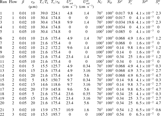
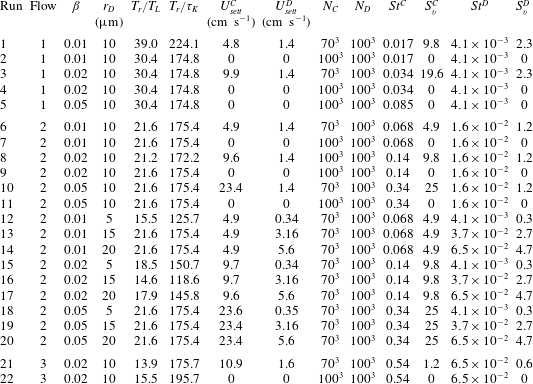
Table 3 lists all the runs discussed in this work. In an effort to understand the different physical effects responsible for the observed collision rates, we have carried out, in addition to more realistic runs in the presence of gravitational settling, a number of simulations without gravity.
Characteristics of the runs discussed here. The second (‘Flow’) column indicates which of the three flows, whose properties are indicated in table 2, is used. The time over which the statistics have been accumulated,
 $T_{r}$
, is compared to
 $T_{L}$
and
 $\unicode[STIX]{x1D70F}_{K}$
, respectively the integral and Kolmogorov time scales. The number of crystals (droplets) used to estimate the statistical properties is
 $N_{C}$
(
 $N_{D}$
). The settling velocity of the crystals (droplets) is denoted by
 $U_{sett}^{C}$
(
 $U_{sett}^{D}$
). In the absence of gravitational settling, the settling velocities
 $U_{sett}^{C}$
and
 $U_{sett}^{D}$
are 0. The Stokes and dimensionless gravity parameters are denoted by
 $St^{C}$
and
 $S_{v}^{C}$
for crystals, and by
 $St^{D}$
and
 $S_{v}^{D}$
for droplets. The ratio
 $r_{D}/a\approx 0.033$
, 0.066, 0.1 and 0.133 for
 $r_{D}=5$
, 10, 15 and
 $20~\unicode[STIX]{x03BC}\text{m}$
, respectively.
Inertial effects play a particularly important role in the study of collisions between small particles in a turbulent flow. These effects can be best quantified by comparing the relaxation times, associated with the translation dynamics of the particles,
 $\unicode[STIX]{x1D70F}_{p}^{C,D}$
, to the time scale of the smallest eddies of the flows, the Kolmogorov time, defined as
 $\unicode[STIX]{x1D70F}_{K}\equiv (\unicode[STIX]{x1D708}/\unicode[STIX]{x1D700})^{1/2}$
. These considerations lead to the introduction of the Stokes numbers,
 $St^{D,C}\equiv \unicode[STIX]{x1D70F}_{p}^{D,C}/\unicode[STIX]{x1D70F}_{K}$
. In the case of droplets, the Stokes number is equal to
 $St^{D}=\unicode[STIX]{x1D70F}_{p}^{D}(r_{D},\unicode[STIX]{x1D70C}_{l})/\unicode[STIX]{x1D70F}_{K}=(2/9)(\unicode[STIX]{x1D70C}_{l}/\unicode[STIX]{x1D70C}_{f})(r_{D}^{2}/\unicode[STIX]{x1D702}^{2})$
. For crystals, one finds, similarly,
 $St^{C}=\unicode[STIX]{x1D70F}_{p}^{C}/\unicode[STIX]{x1D70F}_{K}\approx (4\unicode[STIX]{x1D6FD}/9)(\unicode[STIX]{x1D70C}_{i}/\unicode[STIX]{x1D70C}_{f})(a^{2}/\unicode[STIX]{x1D702}^{2})$
, by using the expression for
 $\unicode[STIX]{x1D70F}_{p}^{C}$
derived in § 2.3.2. The values of the Stokes numbers for the runs carried out here are shown in table 3. Whereas the Stokes numbers associated with the droplets are always very small (less that 0.07), the values of
 $St^{C}$
are of order 0.5 for
 $\unicode[STIX]{x1D6FD}=0.02$
, at the highest turbulence intensity considered. This corresponds to a case where inertial effects become significant (Jucha et al.
Reference Jucha, Naso, Lévêque and Pumir2018).
As gravitational settling is expected to play a significant role in our problem, it also seems appropriate to introduce the dimensionless gravity parameter,
 $S_{v}$
, traditionally defined as the ratio between the expected settling velocity,
 $g\unicode[STIX]{x1D70F}_{p}^{D,C}$
, and the velocity at the size of the smallest eddies,
 $v_{K}=(\unicode[STIX]{x1D700}\unicode[STIX]{x1D708})^{1/4}$
(Grabowski & Vaillancourt Reference Grabowski and Vaillancourt1999). For the ellipsoids, the values of the dimensionless gravity parameters are all larger than 1.2 (for
 $\unicode[STIX]{x1D6FD}=0.02$
and flow 3, with
 $\unicode[STIX]{x1D700}\approx 256~\text{cm}^{2}~\text{s}^{-3}$
). The investigation of collisions between ellipsoids (Jucha et al.
Reference Jucha, Naso, Lévêque and Pumir2018), however, shows that at the highest value of
 $\unicode[STIX]{x1D700}$
considered here, the effect of gravity is actually rather weak. Theoretical considerations, aimed at understanding the orientation distribution of ellipsoids (Gustavsson et al.
Reference Gustavsson, Jucha, Naso, Lévêque, Pumir and Mehlig2017) rather suggest that a more appropriate comparison between the gravitational settling and the turbulence effects is provided by
 $S_{v}^{C}\times R_{\unicode[STIX]{x1D706}}^{-1/2}$
; this suggests a rather weak influence of the gravity at the highest turbulence intensity studied here (
 $S_{v}^{C}\times R_{\unicode[STIX]{x1D706}}^{-1/2}\approx 0.1$
for run 21). The values of the dimensionless gravity parameters for the droplets,
 $S_{v}^{D}$
, shown in table 3, are comparatively smaller, suggesting a weaker role of gravity.
Simulations of particles subject to gravitational settling may lead to unphysical behaviour when the particle settling time becomes shorter than the decorrelation time of the flow (Ireland, Bragg & Collins Reference Ireland, Bragg and Collins2016). In the present work, the smallest values of the ratio between the typical settling time of crystals,
 $L_{B}/U_{sett}^{C}$
, where
 $L_{B}$
is the linear size of the computational domain, and the decorrelation time of the flow,
 $T_{L}$
, are 1.3 when
 $\unicode[STIX]{x1D700}\approx 1~\text{cm}^{2}~\text{s}^{-3}$
and
 $\unicode[STIX]{x1D6FD}=0.02$
, and 1.5 when
 $\unicode[STIX]{x1D700}\approx 15~\text{cm}^{2}~\text{s}^{-3}$
and
 $\unicode[STIX]{x1D6FD}=0.05$
. These values are all larger than 1. As droplets settle much slower, the ratios
 $L_{B}/(T_{L}U_{sett}^{D})$
are even smaller. For these reasons, we do not expect the finite vertical size of our computational domain to be a concern in the present work.
2.5 Collision detection and analysis
2.5.1 Definitions
We begin by recalling that we are restricting here to the ghost-particle approximation of the geometric collision rate, obtained by counting when particles come into contact. With this convention, the number of collisions
 $N_{coll}$
between
 $N_{D}$
droplets and
 $N_{C}$
crystals in a volume
 $V$
during a time
 $T$
is proportional to
 $N_{D}\times N_{C}$
, to
 $1/V$
and to
 $T$
. It can therefore be expressed as
 $$\begin{eqnarray}N_{coll}=K_{DC}\times \frac{N_{D}\times N_{C}}{V}\times T,\end{eqnarray}$$
where the proportionality coefficient
 $K_{DC}$
has the dimension of a flux (
 $\text{cm}^{3}~\text{s}^{-1}$
in physical units) and is commonly referred to as the collision kernel or collision rate (Pumir & Wilkinson Reference Pumir and Wilkinson2016). It is expected to depend on the particles’ geometry, on the carrier flow characteristics and on the gravity magnitude.
This collision rate, which is effectively the flux of droplets impacting the crystals, can be simply estimated as the product of the difference between the settling velocities between the two types of particles, and the area of the largest sides of the ellipsoids,
 $\unicode[STIX]{x03C0}a^{2}$
, times a dimensionless coefficient
 $E_{DC}$
, the turbulence enhancement factor (Grabowski & Wang Reference Grabowski and Wang2013). The latter quantity is therefore defined as
 $$\begin{eqnarray}E_{DC}=\frac{K_{DC}}{\unicode[STIX]{x03C0}|U_{sett}^{C}-U_{sett}^{D}|a^{2}},\end{eqnarray}$$
where
 $U_{sett}^{C}$
(
 $U_{sett}^{D}$
) is the mean crystal (droplet) settling velocity. In the present problem, the factor
 $E_{DC}$
takes into account in particular the effect of the crystal orientation. We note that our definition of
 $E_{DC}$
neglects the radius
 $r_{D}$
of the droplets compared to the semi-axis
 $a$
of the crystal.
We conclude this subsection by mentioning that the modifications of the flow close to the collision time is in principle taken into account by an effective parameter, the collision efficiency (Pruppacher & Klett Reference Pruppacher and Klett1997; Wang & Ji Reference Wang and Ji2000; Grabowski & Wang Reference Grabowski and Wang2013).
2.5.2 Collision detection method
Collisions are identified by using the ‘ghost-collision’ approximation, which consists in tracking the particles’ positions and in simply detecting when two of them come into contact, without modifying their subsequent dynamics (Sundaram & Collins Reference Sundaram and Collins1996). This method has been tested in the case of collisions between spherical particles (Sundaram & Collins Reference Sundaram and Collins1996; Voßkuhle et al. Reference Voßkuhle, Lévèque, Wilkinson and Pumir2013; Pumir & Wilkinson Reference Pumir and Wilkinson2016), and more recently used for detecting collisions between ellipsoidal objects (Siewert et al. Reference Siewert, Kunnen, Meinke and Schröder2014a ; Siewert, Kunnen & Schröder Reference Siewert, Kunnen and Schröder2014b ; Jucha et al. Reference Jucha, Naso, Lévêque and Pumir2018).
The method that we employed for identifying contacts between the ellipsoidal crystals and the spherical droplets, inspired from Choi et al. (Reference Choi, Chang, Wang, Kim and Elber2009), is the same as that of Siewert et al. (Reference Siewert, Kunnen, Meinke and Schröder2014a ,Reference Siewert, Kunnen and Schröder b ) and Jucha et al. (Reference Jucha, Naso, Lévêque and Pumir2018). Further details are presented in appendix A. It consists in computing, at each time and for each pair of particles, the roots of a fourth-order polynomial defined as a function of matrices characterizing the particles’ surfaces. The nature of these roots provides a way to distinguish situations when the two particles are separated, overlap or are in contact. More details on the algorithm can be found in Siewert et al. (Reference Siewert, Kunnen and Schröder2014b ,Reference Siewert, Kunnen and Schröder c ) and Jucha et al. (Reference Jucha, Naso, Lévêque and Pumir2018).
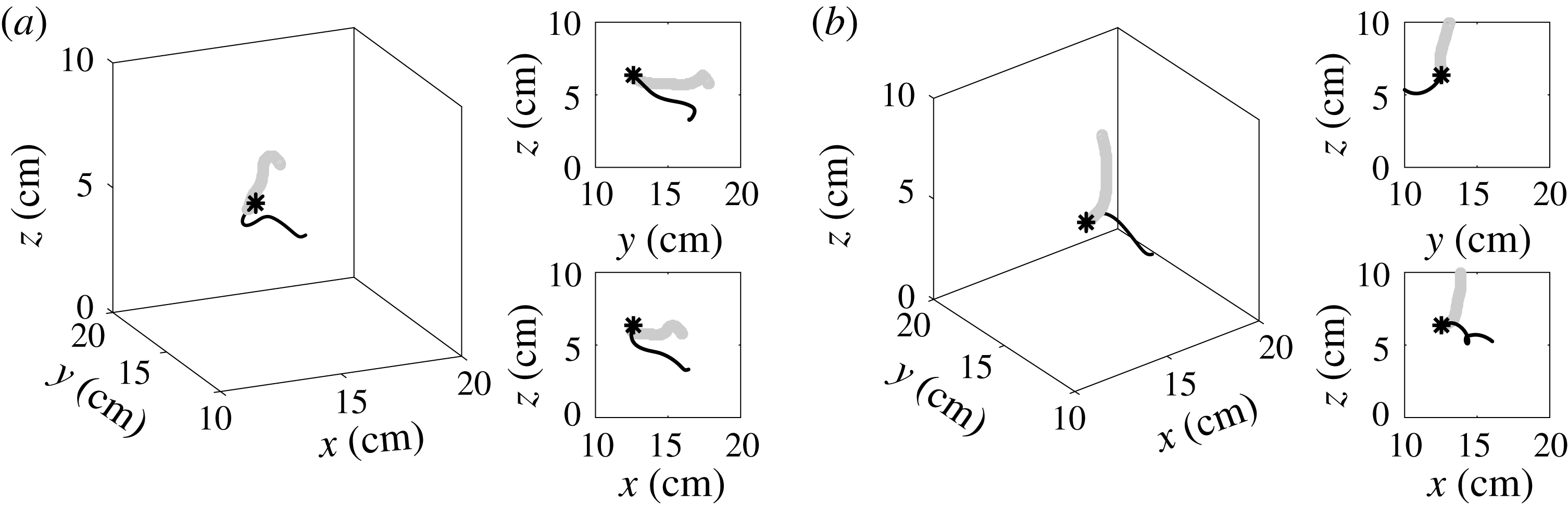
As an illustration, the trajectories of two pairs of crystals and droplets before their collisions are shown in figure 1. The trajectories are taken from run 21, with
 $\unicode[STIX]{x1D700}\approx 256~\text{cm}^{2}~\text{s}^{-3}$
, in the presence of gravity. Owing to the larger settling velocity of the crystals in this case, most collisions occur with the droplet underneath the crystal.
Two examples of trajectories of crystals (thick grey line) and droplets (thin black line) before their collisions, indicated by stars, and their projections on two vertical planes. Only the centre of the computational domain is shown. Gravity is aligned with the
 $z$
direction and is pointing towards
 $z<0$
.

2.5.3 Data analysis
To check the reliability of the determined collision rates, we have estimated them by partitioning our long runs into smaller ones, of duration
 ${\approx}25\unicode[STIX]{x1D70F}_{K}$
, and measured the fluctuations of the collision rate estimated over the shorter runs. Aside for a few runs, where they were as high as
 ${\sim}10\,\%$
(run 3), the fluctuations were in most cases of the order of a few per cent. Given that the runs are at the minimum
 $125\unicode[STIX]{x1D70F}_{K}$
, we estimate the error bars to be of the order of 1 %, with the exception of run 3, where we estimate it to be no larger than 5 %.
2.6 Limitations of our approach
It should be kept in mind that (2.12) and (2.14) are obtained by completely neglecting the inertia of the fluid, i.e. by assuming the Reynolds numbers to be very small, and by solving the Stokes equations (Happel & Brenner Reference Happel and Brenner1983). Taking into account the fluid inertia effects in a systematic expansion in the Reynolds number is a challenging task (Cox Reference Cox1965; Khayat & Cox Reference Khayat and Cox1989). So far, a tractable and well-accepted model describing the translational and rotational motion of any spheroid and accounting for inertial effects is not available, even in the simplest case of weak inertia. The corrections induced by fluid inertia (finite Reynolds-number effects) have been recently studied in the case of prolate spheroids (Lopez & Guazzelli Reference Lopez and Guazzelli2017). The investigation of these effects in the case of oblate spheroids should be the subject of future work; see also Gustavsson et al. (Reference Gustavsson, Jucha, Naso, Lévêque, Pumir and Mehlig2017).
Furthermore, in the present approach the dynamics of the particles are assumed to obey a one-way coupling, that is (i) the modification of the flow by these objects and (ii) their interactions are not taken into account. Accounting for these two effects would necessitate the use of particle-resolved methods (see e.g. Lucci, Ferrante & Elghobashi Reference Lucci, Ferrante and Elghobashi2010; Naso & Prosperetti Reference Naso and Prosperetti2010; Homann, Bec & Grauer Reference Homann, Bec and Grauer2013; Wang et al. Reference Wang, Ayala, Gao, Andersen and Mathews2014; Chouippe & Uhlmann Reference Chouippe and Uhlmann2015). For the problem of interest, such methods would be tractable only at low values of the Reynolds numbers and would certainly not allow well-converged statistics of collisions to be obtained.
Another limitation of the present approach is that it does not account for the possible modification of the crystals’ and droplets’ geometry, and thereby their subsequent dynamics after a collision. This issue would necessitate separate studies. In fact, the outcome of a collision depends on a number of parameters: the crystals and droplets could conceivably bounce elastically, or bounce with a restitution coefficient
 $e$
(
 $e\leqslant 1$
). Alternatively, they could aggregate and form a larger object with a complex shape. This is well known in cloud physics, where the unknown effect of hydrodynamic interactions (and molecular forces) is parametrized by a ‘collision efficiency’ parameter. This parameter is difficult to estimate from first principles, even in the case of spheres (see e.g. Chun & Koch Reference Chun and Koch2005).
Finally, as already mentioned, the chosen values of the parameters characterizing the particles and the small space and time scales of the flow are physically relevant to the microphysics of clouds at
 $T=-20\,^{\circ }\text{C}$
, but the Reynolds numbers considered are much smaller than in real flows. This might lead to an underestimate of the influence of velocity gradient fluctuations on the statistical properties of the crystals’ orientation.
3 Settling velocities of droplets and crystals in turbulent flows
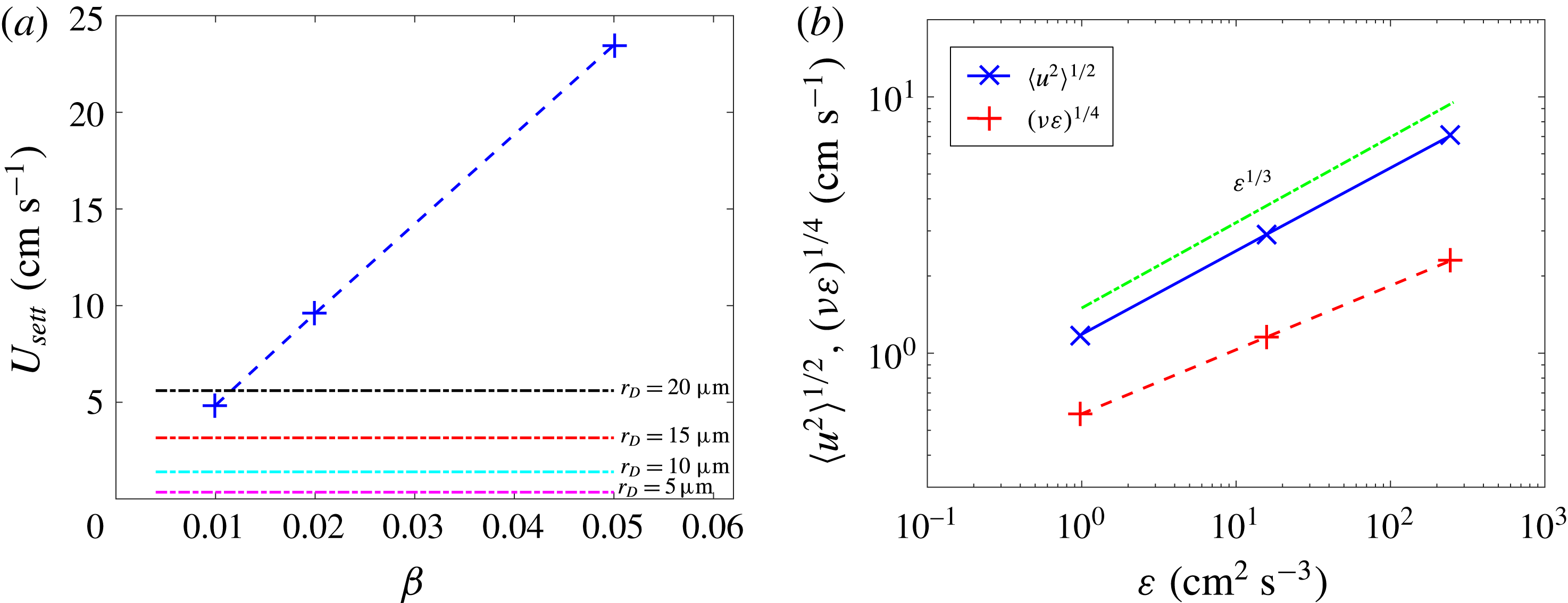
The mean settling velocity of the crystals
 $U_{sett}^{C}$
is plotted in figure 2(a) as a function of
 $\unicode[STIX]{x1D6FD}$
, for flow 2 (
 $\unicode[STIX]{x1D700}\approx 16~\text{cm}^{2}~\text{s}^{-3}$
). The dependence of the velocity
 $U_{sett}^{C}$
on
 $\unicode[STIX]{x1D700}$
, over the range of values considered in this study, is found to be small. Based on this figure,
 $U_{sett}^{C}$
is roughly proportional to
 $\unicode[STIX]{x1D6FD}$
. This can be qualitatively understood with (2.15), which implies that, at a fixed orientation of the ellipsoid, and in a fluid at rest, the settling velocity of the ellipsoids varies proportionally to
 $\unicode[STIX]{x1D6FD}$
, that is, to the mass of the crystal. In a turbulent flow, it was shown (Jucha et al.
Reference Jucha, Naso, Lévêque and Pumir2018) that: (i)
 $U_{sett}^{C}$
increases slightly with
 $\unicode[STIX]{x1D700}$
(for
 $\unicode[STIX]{x1D6FD}=0.02$
it was found to be
 ${\approx}9.9~\text{cm}~\text{s}^{-1}$
for flows 1 and 2, and
 ${\approx}10.4~\text{cm}~\text{s}^{-1}$
for flow 3), and (ii) for a given value of the turbulence intensity, ellipsoids settle faster as their largest face is more aligned with gravity. This can be simply understood as a consequence of the variation of the resistance as a function of the orientation of the crystals. The latter effect was found to be stronger at larger turbulence intensity. These results will be useful to interpret the efficiency of the collisions between droplets and crystals (see § 5.1).
Characteristic velocities in the problem. (a) Settling velocity of the ellipsoids as a function of
 $\unicode[STIX]{x1D6FD}$
(blue dashed line), for flow 2 (
 $\unicode[STIX]{x1D700}\approx 16~\text{cm}^{2}~\text{s}^{-3}$
). The settling velocity is proportional to
 $\unicode[STIX]{x1D6FD}$
, i.e. to the mass of the ellipsoids. For comparison, the settling velocities of the droplets are shown as dashed-dotted lines at the four values of the droplet radius
 $r_{D}$
indicated. (b) The characteristic velocity of the smallest eddies (red dashed line), and the root-mean-square of the velocity fluctuations of the turbulent flow (blue solid line), as functions of
 $\unicode[STIX]{x1D700}$
. The green dashed-dotted line shows the dependence on
 $\unicode[STIX]{x1D700}$
expected for
 $\langle \boldsymbol{u}^{2}\rangle ^{1/2}$
,
 $\langle \boldsymbol{u}^{2}\rangle ^{1/2}\propto \unicode[STIX]{x1D700}^{1/3}$
, which is slightly faster than
 $\unicode[STIX]{x1D700}^{1/4}$
(red dashed line).

The settling velocity of the droplets,
 $U_{sett}^{D}$
, also shown in figure 2(a) for the different values of
 $r_{D}$
considered here, grows as
 $\propto r_{D}^{2}$
. This is an elementary consequence of (2.4) and (2.5). It can be noted that
 $U_{sett}^{D}$
is generally lower than that of the crystals. The only exception is provided by the largest droplets (
 $r_{D}=20~\unicode[STIX]{x03BC}\text{m}$
) and the slimmest ellipsoids (
 $\unicode[STIX]{x1D6FD}=0.01$
); see table 3, run 14. Moreover, table 3 suggests that increasing the turbulence level slightly enhances the settling velocity of the droplets (compare e.g. runs 1, 6 and 21), in qualitative agreement with previous works (Ayala et al.
Reference Ayala, Rosa, Wang and Grabowski2008).
Finally, we have plotted in figure 2(b) the characteristic velocities of the carrier flow as a function of
 $\unicode[STIX]{x1D700}$
. The variance of the velocity fluctuations
 $\langle \boldsymbol{u}^{2}\rangle$
grows as
 $\propto \unicode[STIX]{x1D700}^{2/3}$
, as a consequence of the relation
 $\langle \boldsymbol{u}^{2}\rangle \propto (\unicode[STIX]{x1D700}L)^{2/3}$
(
 $L$
is the integral length scale of the flow), valid for homogeneous and isotropic turbulence, and of the fact that
 $L$
does not vary significantly in our simulations. The typical velocity increment between two points of the flow separated by a distance
 $\unicode[STIX]{x1D702}$
,
 $v_{K}=(\unicode[STIX]{x1D700}\unicode[STIX]{x1D708})^{1/4}$
, obviously behaves as
 $\unicode[STIX]{x1D700}^{1/4}$
.
4 Collision rate between crystals and droplets
This section is devoted to the analysis of the collision rate between crystals and droplets. We will investigate in particular its dependence on the particles’ geometry and mass, and on turbulence intensity. Results obtained in the absence of gravity will allow us to disentangle the effects of gravitational settling and of turbulence.
4.1 Dependence on the aspect ratio of the crystal,
 $\unicode[STIX]{x1D6FD}$

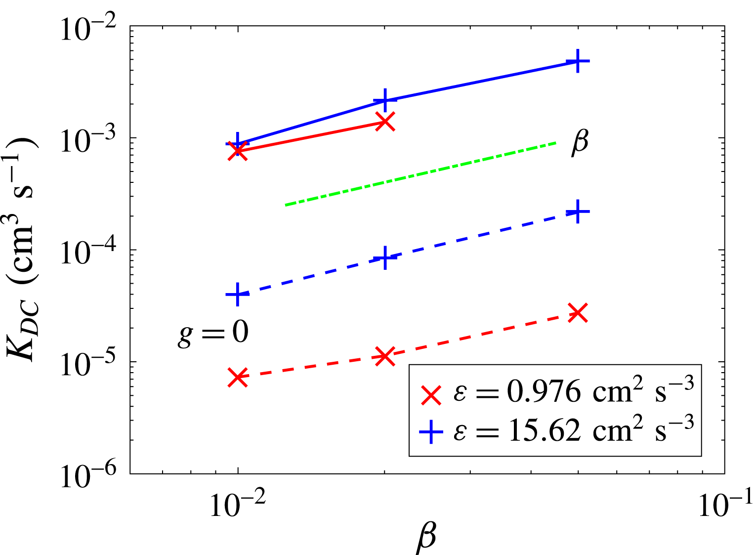
Dependence of the collision rate between droplets and crystals on the aspect ratio of the ellipsoids
 $\unicode[STIX]{x1D6FD}$
(or, equivalently, on its mass), for flow 1 (
 $\unicode[STIX]{x1D700}\approx 1~\text{cm}^{2}~\text{s}^{-3}$
; ‘
 $\times$
’ symbols) and flow 2 (
 $\unicode[STIX]{x1D700}\approx 16~\text{cm}^{2}~\text{s}^{-3}$
; ‘
 $+$
’ symbols), in the presence (full curves) and in the absence (dashed curves) of gravitational settling. In all cases, the dependence of the collision rate is approximately linear with
 $\unicode[STIX]{x1D6FD}$
. All the curves shown here correspond to
 $r_{D}=10~\unicode[STIX]{x03BC}\text{m}$
.

Figure 3 shows the collision rate
 $K_{DC}$
, defined in § 2.5.1, as a function of
 $\unicode[STIX]{x1D6FD}$
, for
 $r_{D}=10~\unicode[STIX]{x03BC}\text{m}$
and two flows (1 and 2), both in the presence and in the absence of gravity. In all cases, the collision rate grows roughly linearly with
 $\unicode[STIX]{x1D6FD}$
.
Figure 3 clearly shows that the collision rate increases with the turbulence level. At the values of
 $\unicode[STIX]{x1D700}$
shown in figure 3, the collision rate is much larger in the presence of gravitational settling than without it. In the context of cloud microphysics, this implies that the collision rate is dominated, at low values of
 $\unicode[STIX]{x1D700}$
, by the effect of differential settling.
It is important to stress here that the dependence on
 $\unicode[STIX]{x1D6FD}$
of
 $K_{DC}$
, discussed in this subsection, amounts to a dependence on the mass of the crystal. This is a consequence of the choice made here of considering crystals of fixed semi-axis
 $a$
and density
 $\unicode[STIX]{x1D70C}_{i}$
(see table 1), which implies that the volume, hence the mass, of the crystals is simply proportional to
 $\unicode[STIX]{x1D6FD}$
.
4.2 Dependence on the turbulence intensity
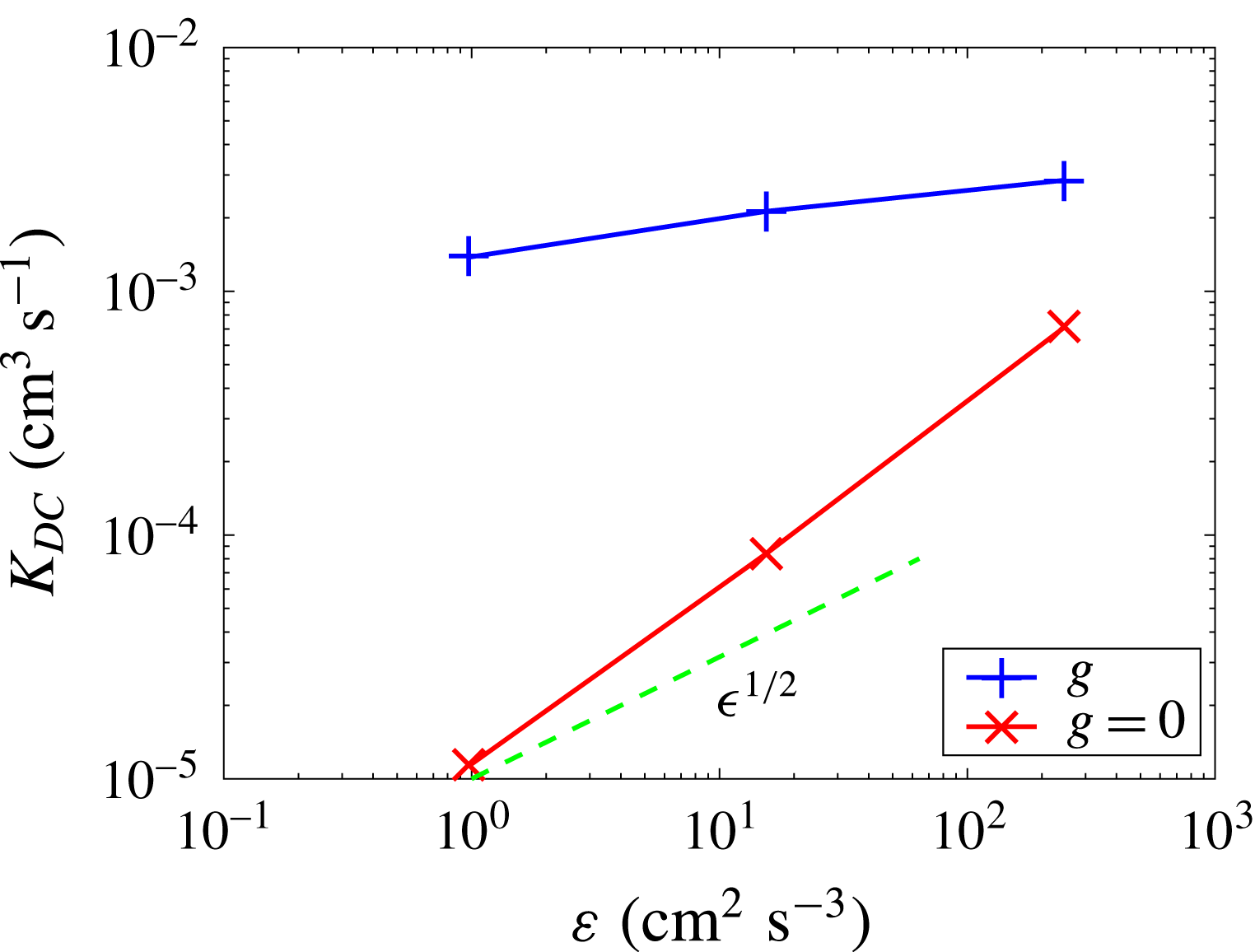
Dependence of the collision rate on the turbulence intensity, with (‘
 $+$
’ symbols) and without (‘
 $\times$
’ symbols) gravitational settling. The collision rate is much larger in the presence of gravitational settling, although the relative difference with the collision rate without gravitational settling diminishes as the turbulence intensity is increased. The results shown here correspond to
 $\unicode[STIX]{x1D6FD}=0.02$
and
 $r_{D}=10~\unicode[STIX]{x03BC}\text{m}$
.

The dependence of the collision kernel
 $K_{DC}$
on the turbulence rate is shown in figure 4, for
 $\unicode[STIX]{x1D6FD}=0.02$
and
 $r_{D}=10~\unicode[STIX]{x03BC}\text{m}$
. In the presence of gravity,
 $K_{DC}$
hardly changes with
 $\unicode[STIX]{x1D700}$
, thereby suggesting that the collision process is then essentially driven by gravitational settling. As already noted in the previous subsection, the collision rate between crystals and droplets is much weaker in the absence of gravity. In that case, collisions occur much more frequently, as expected, as the turbulence intensity is increased. As a consequence, the difference between the two regimes (with and without gravity) diminishes at increasing
 $\unicode[STIX]{x1D700}$
.
These observations raise the question whether gravitational settling remains the dominant effect leading to collisions when
 $\unicode[STIX]{x1D700}>256~\text{cm}^{2}~\text{s}^{-3}$
. In this context, we mention that an even more pronounced increase in the collision rate in the absence of gravity was also observed in a turbulent monodisperse suspension of crystals (Jucha et al.
Reference Jucha, Naso, Lévêque and Pumir2018). We also recall that, at a fixed turbulence rate and particle geometry, gravitational settling tends to reduce the collision rate in a monodisperse suspension of spherical particles (Grabowski & Vaillancourt Reference Grabowski and Vaillancourt1999; Falkovich & Pumir Reference Falkovich and Pumir2007; Ayala et al.
Reference Ayala, Rosa, Wang and Grabowski2008).
4.3 Dependence on the droplet size
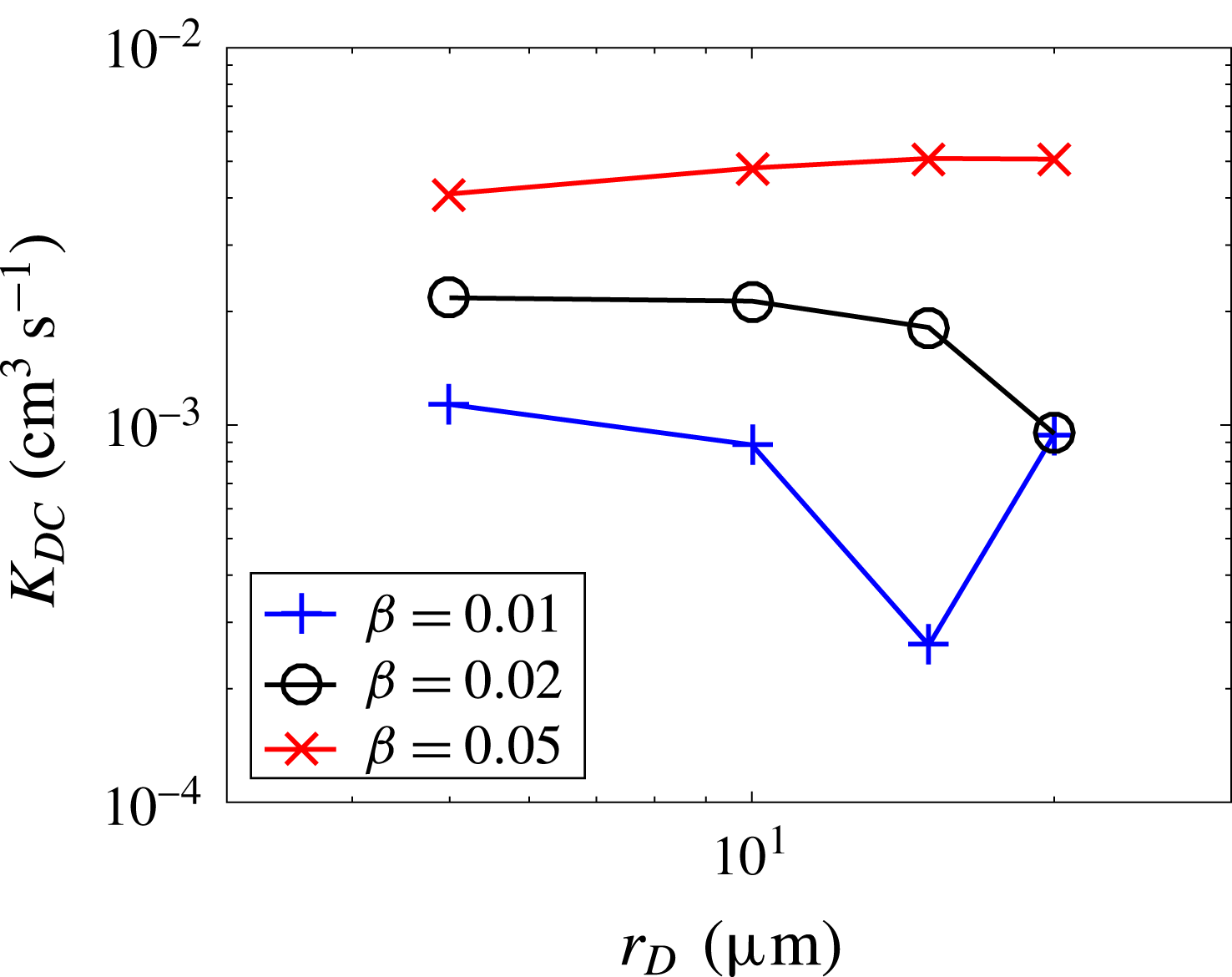
The collision kernel between crystals and droplets is plotted as a function of the droplet radius
 $r_{D}$
in figure 5, for the three values of
 $\unicode[STIX]{x1D6FD}$
considered. The variation of
 $K_{DC}$
with
 $r_{D}$
strongly depends on
 $\unicode[STIX]{x1D6FD}$
: the collision kernel is virtually independent on
 $r_{D}$
for the thickest ellipsoids (
 $\unicode[STIX]{x1D6FD}=0.05$
), whereas it exhibits a non-monotonic dependence on this parameter for
 $\unicode[STIX]{x1D6FD}=0.01$
. In the latter case, one observes a very significant dip of the collision rate, as
 $r_{D}$
increases, at
 $r_{D}\approx 15~\unicode[STIX]{x03BC}\text{m}$
. The values of the collision rate are very close for
 $r_{D}=10~\unicode[STIX]{x03BC}\text{m}$
and for
 $r_{D}=20~\unicode[STIX]{x03BC}\text{m}$
. Interestingly, the very abrupt change of
 $K_{DC}$
as
 $r_{D}$
varies occurs when the settling velocity of crystals becomes smaller than that of droplets (see figure 2
a). Namely, the settling velocity of spheres with
 $r_{D}=20~\unicode[STIX]{x03BC}\text{m}$
is larger than that of ellipsoids with
 $\unicode[STIX]{x1D6FD}=0.01$
, while in all other cases ellipsoids settle faster than spheres. As documented in § 5.1, this significantly influences the mechanisms of collision.
5 Collision mechanisms
Dependence of the collision rate on the droplet size,
 $r_{D}$
, for three different crystal shapes,
 $\unicode[STIX]{x1D6FD}=0.01$
(
 $+$
),
 $\unicode[STIX]{x1D6FD}=0.02$
(○) and
 $\unicode[STIX]{x1D6FD}=0.05$
(
 $\times$
), for flow 2 (
 $\unicode[STIX]{x1D700}\approx 16~\text{cm}^{2}~\text{s}^{-3}$
). The collision rate
 $K_{DC}$
is essentially independent of
 $r_{D}$
for
 $\unicode[STIX]{x1D6FD}=0.05$
. In contrast, a sharp drop is observed when
 $\unicode[STIX]{x1D6FD}=0.01$
for
 $r_{D}\approx 15~\unicode[STIX]{x03BC}\text{m}$
, before returning to a large value for
 $r_{D}=20~\unicode[STIX]{x03BC}\text{m}$
.

In a suspension of droplets and ellipsoids, the difference between the settling velocities of the droplets and the ellipsoids is expected to play a role in the collision rate. Figure 4 indeed shows that, in the absence of gravitational settling, the collision rate is smaller, by approximately an order of magnitude, than with settling. The difference, however, becomes weaker when the Reynolds number increases. As we explain in this section, this is due to another mechanism, related to the inertia of the particles, which becomes important at higher turbulence intensity. We discuss in this section the corresponding mechanisms, responsible for the collisions between droplets and crystals.
5.1 Collisions induced by the relative settling velocity between light crystals and droplets
Section 3, see in particular figure 2(a), shows that, as expected, the settling velocity becomes larger when the size of the droplets increases, or when the mass of the crystals (i.e.
 $\unicode[STIX]{x1D6FD}$
) increases. With the exception of case when
 $\unicode[STIX]{x1D6FD}=0.01$
and
 $r_{D}=20~\unicode[STIX]{x03BC}\text{m}$
, the crystals settle faster than the droplets.
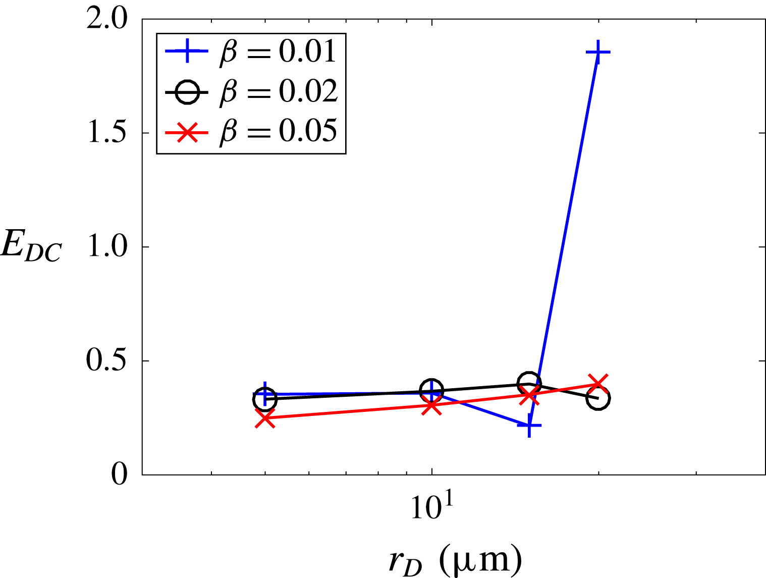
The turbulent enhancement factor,
 $E_{DC}$
, defined by (2.17), corresponding to the data shown in figure 5. Whereas the collision rate is approximately constant in all cases where the settling velocity of the crystals exceeds the settling velocity of the droplets, the turbulent enhancement factor jumps to a much higher value in the opposite case. The data shown here correspond to
 $\unicode[STIX]{x1D700}\approx 16~\text{cm}^{2}~\text{s}^{-3}$
.

Assuming that collisions are induced by differential settling between crystals and droplets, the collision rate
 $K_{DC}$
can be written as
 $\unicode[STIX]{x03C0}a^{2}|U_{sett}^{C}-U_{sett}^{D}|$
times a numerical prefactor
 $E_{DC}$
, the turbulent enhancement factor, defined by (2.17).
Figure 6 shows the turbulent enhancement factor obtained for
 $\unicode[STIX]{x1D6FD}=0.01$
(
 $+$
’),
 $\unicode[STIX]{x1D6FD}=0.02$
(○) and
 $\unicode[STIX]{x1D6FD}=0.05$
(
 $\times$
), as functions of
 $r_{D}$
. Remarkably,
 $E_{DC}$
is approximately constant for all the runs in the presence of gravitational settling, for which
 $U_{sett}^{C}>U_{sett}^{D}$
. The value of
 $E_{DC}$
is then found to be
 ${\approx}0.3{-}0.4$
. In contrast, the turbulent enhancement factor jumps to a much higher value when
 $U_{sett}^{C}<U_{sett}^{D}$
,
 $E_{DC}\approx 1.9$
.
The difference between values of the turbulent enhancement factor
 $E_{DC}<1$
when
 $U_{sett}^{C}>U_{sett}^{D}$
, and values
 $E_{DC}>1$
when
 $U_{sett}^{C}<U_{sett}^{D}$
, can be qualitatively understood by the following elementary considerations, which rest on the interpretation of the collision rate as a flux of droplets impacting the ellipsoids. To estimate this flux, we simply consider the volume swept by a crystal moving through an assembly of droplets, and consider a frame, moving at a velocity
 $U_{sett}^{D}$
, such that the centre of mass of the droplets is at rest. In the present phenomenological considerations, we neglect the variation in the vertical component of the droplet velocity.
It is important to recall here that the settling velocity of the ellipsoids depends on their orientation: ellipsoids settle faster with their edges first. We will define
 $\boldsymbol{n}$
as the unit vector aligned with the minor axis of an ellipsoid and
 $n_{z}$
its projection on
 $\boldsymbol{e}_{z}=\boldsymbol{g}/|\boldsymbol{g}|$
(by symmetry the sign of
 $n_{z}$
is immaterial, we will therefore assume that
 $n_{z}>0$
). One can observe that an ellipsoid settling at a velocity
 $\boldsymbol{v}(n_{z})$
, relative to droplets, sweeps per unit time a volume equal to
 $\unicode[STIX]{x03C0}a^{2}\times n_{z}\times |v_{z}(n_{z})|$
.
In the case where
 $U_{sett}^{C}>U_{sett}^{D}$
(crystals settling faster than droplets), we approximate the volume swept by the crystals by conditioning on the orientation,
 $n_{z}$
, and by estimating the difference in settling velocities between crystals and droplets as
 $v_{z}(n_{z})=\langle v_{z}^{C}|n_{z}\rangle -U_{sett}^{D}$
, where
 $\langle v_{z}^{C}|n_{z}\rangle$
is the settling velocity of the crystals conditioned on the orientation,
 $n_{z}$
. With our conventions,
 $v_{z}$
,
 $\langle v_{z}^{C}|n_{z}\rangle$
and
 $U_{sett}^{D}$
are all positive quantities. It has been documented that when
 $n_{z}$
increases from
 $n_{z}=0$
to
 $n_{z}=1$
, the conditional velocity
 $\langle v_{z}^{C}|n_{z}\rangle$
decreases (Siewert et al.
Reference Siewert, Kunnen and Schröder2014c
; Gustavsson et al.
Reference Gustavsson, Jucha, Naso, Lévêque, Pumir and Mehlig2017; Jucha et al.
Reference Jucha, Naso, Lévêque and Pumir2018), so the relative velocity between crystals and droplets diminishes. This implies that the flux of droplets between crystals and droplets results from a competition between the horizontal projection of the large face of an ellipsoid
 $\unicode[STIX]{x03C0}a^{2}n_{z}$
(maximized when
 $n_{z}$
is increased) and the settling velocities
 $\langle v_{z}^{C}|n_{z}\rangle$
(maximized when
 $n_{z}$
is decreased). This results in a relatively low turbulent enhancement factor,
 $E_{DC}<1$
. It is also known (Siewert et al.
Reference Siewert, Kunnen and Schröder2014c
; Gustavsson et al.
Reference Gustavsson, Jucha, Naso, Lévêque, Pumir and Mehlig2017; Jucha et al.
Reference Jucha, Naso, Lévêque and Pumir2018) that, in the regime of parameters and with the equations of motion considered in this work, the orientation of ellipsoids settling with their edge first is more probable than with the edge horizontal.
In the opposite case, when
 $U_{sett}^{C}<U_{sett}^{D}$
, the crystals move up in a frame where the droplets are at rest, so the volume swept per unit of time is
 $\unicode[STIX]{x03C0}a^{2}n_{z}\times (U_{sett}^{D}-\langle v_{z}^{C}|n_{z}\rangle )$
. The quantity
 $U_{sett}^{D}-\langle v_{z}^{C}|n_{z}\rangle$
increases when
 $n_{z}$
increases from 0 to 1. As a result, crystals with their base perpendicular to gravity maximize the collision rate since this configuration maximizes both the horizontal projection of the large face of the ellipsoid and the relative velocity
 $U_{sett}^{D}-\langle v_{z}^{C}|n_{z}\rangle$
. This implies that the slow settling crystals, with
 $n_{z}\approx 1$
, contribute more than the fast settling ones. As a result, the turbulent enhancement factor
 $E_{DC}>1$
.
As shown in Gustavsson et al. (Reference Gustavsson, Jucha, Naso, Lévêque, Pumir and Mehlig2017) and Jucha et al. (Reference Jucha, Naso, Lévêque and Pumir2018), the distribution of orientation strongly varies over the range of values of
 $\unicode[STIX]{x1D6FD}$
considered here. The lack of dependence of the turbulent enhancement factor on
 $\unicode[STIX]{x1D6FD}$
therefore suggests that the distribution of the orientation of the settling ellipsoids does not affect
 $E_{DC}$
much. This is particularly important, as it has been suggested (Cox Reference Cox1965; Pruppacher & Klett Reference Pruppacher and Klett1997) that fluid inertia favours a different orientation of settling crystals, with a maximum for
 $n_{z}=1$
.
Numerically, we investigated the statistics of orientation of colliding ellipsoids with
 $\unicode[STIX]{x1D6FD}=0.01$
. We observed that, except in the case
 $r_{D}=15~\unicode[STIX]{x03BC}\text{m}$
, the distribution is significantly biased towards values of
 $n_{z}$
close to 1. This can be understood from the simple following argument. Even in the case where crystals settle faster than droplets, and provided the difference in settling velocity
 $U_{sett}^{C}-U_{sett}^{D}$
is large enough, the influence of the explicit contribution of
 $n_{z}$
in the expression of the volume swept by the crystal plays a more important role than the dependence of the settling velocity of the crystals on
 $n_{z}$
. This leads, in practice to the same qualitative result as in the case where crystals settle slower than droplets (
 $\unicode[STIX]{x1D6FD}=0.01$
,
 $r_{D}=20~\unicode[STIX]{x03BC}\text{m}$
).
The collision rates for droplets of size
 $r_{D}=10~\unicode[STIX]{x03BC}\text{m}$
and for crystals with
 $\unicode[STIX]{x1D6FD}=0.02$
in the presence of gravity (‘
 $+$
’ symbols in figure 4) seem to be relatively independent of
 $\unicode[STIX]{x1D700}$
. Similarly, the settling velocities of crystals with
 $\unicode[STIX]{x1D6FD}=0.02$
and droplets of size
 $r_{D}=10~\unicode[STIX]{x03BC}\text{m}$
do not vary much, which explains why the collision efficiency does not vary much as a function of
 $\unicode[STIX]{x1D700}$
over the range studied here.
5.2 Effect of increased turbulence intensity on the collision rate
Whereas the collision rate in the presence of settling does not depend much on the turbulence intensity (
 $\unicode[STIX]{x1D700}$
or equivalently
 $R_{\unicode[STIX]{x1D706}}$
; see the ‘
 $+$
’ symbols in figure 4), the collision rate in the absence of any settling grows very dramatically when
 $\unicode[STIX]{x1D700}$
increases (see the ‘
 $\times$
’ symbols in figure 4). We provide in this section an elementary analysis of the role of turbulence.
As turbulence strongly increases velocity gradients in a fluid, it enhances the probability of two particles to get within a small distance away from each other. The seminal work of Saffman & Turner (Reference Saffman and Turner1956) provides an estimate of the collision rate, based on the velocity difference between two colliding particles for which inertial effects are negligible. In the case of a monodisperse solution of spherical particles of diameter
 $d=2r_{D}$
, the predicted collision rate is
 $K_{turb}\propto d^{3}|\unicode[STIX]{x1D735}\boldsymbol{u}|\propto d^{3}/\unicode[STIX]{x1D70F}_{K}$
. Qualitatively, the collision rate is merely the product of the area
 ${\approx}r_{D}^{2}$
of a sphere of radius
 $2r_{D}$
surrounding the centre of a particle, times the relative velocity
 ${\approx}r_{D}/\unicode[STIX]{x1D70F}_{K}$
of the two spheres. Without going into complicated algebra, in the present case, dimensional analysis indicates that the collision rate should be of the order
 $a^{3}/\unicode[STIX]{x1D70F}_{K}$
. As the Kolmogorov time
 $\unicode[STIX]{x1D70F}_{K}\approx (\unicode[STIX]{x1D708}/\unicode[STIX]{x1D700})^{1/2}$
, the expected dependence of the collision rate, based on these estimates, is
 $K_{DC}\propto a^{3}(\unicode[STIX]{x1D700}/\unicode[STIX]{x1D708})^{1/2}$
.
The collision rates shown in figure 4 in the absence of gravitational settling (see curve with the ‘
 $\times$
’ symbols) grows in fact faster than
 $\unicode[STIX]{x1D700}^{1/2}$
. The range of validity of the Saffman–Turner estimate does not exceed
 $St\approx 0.1$
or so. At higher values of the Stokes number, the preferential concentration effect or the influence of caustics plays an important role (Gustavsson & Mehlig Reference Gustavsson and Mehlig2011; Bragg & Collins Reference Bragg and Collins2014b
,Reference Bragg and Collins
a
; Voßkuhle et al.
Reference Voßkuhle, Pumir, Lévêque and Wilkinson2014; Pumir & Wilkinson Reference Pumir and Wilkinson2016). In the case of crystals with
 $\unicode[STIX]{x1D6FD}=0.02$
, the Stokes number is
 $St^{C}\approx 0.14$
at
 $\unicode[STIX]{x1D700}\approx 16~\text{cm}^{2}~\text{s}^{-3}$
; see table 3. In this context, it is natural to observe a growth of the collision rate, see figure 4, faster than
 $\unicode[STIX]{x1D700}^{1/2}$
over the range of values of
 $\unicode[STIX]{x1D700}$
studied here.
With our choice of parameters, the values of
 $St^{D}$
, the Stokes number of the droplets, are very small (
 $St^{D}\lesssim 0.065$
, see table 3). This implies that the droplets closely follow the flow. The situation would change at higher turbulence intensity. For example, with an energy dissipation rate
 $\unicode[STIX]{x1D700}\approx 10\,000~\text{cm}^{2}~\text{s}^{-3}$
, the Stokes number for particles of size
 $10~\unicode[STIX]{x03BC}\text{m}$
would become of order
 $St^{D}\approx 0.4$
, resulting in significant inertial effects (Voßkuhle et al.
Reference Voßkuhle, Pumir, Lévêque and Wilkinson2014; Pumir & Wilkinson Reference Pumir and Wilkinson2016), and plausibly in a further enhancement of the collision rate.
6 Where do droplets impact ellipsoids?
As we show in this section, determining where the droplets hit the ellipsoids during collisions provides important information on the collision mechanisms. The issue is also relevant to the underlying cloud physics problem, to understand how crystals grow as they collide with droplets (riming). In this problem, gravitational settling clearly plays a very significant role. We begin by studying the seemingly unrelated problem of the impact of droplets on ellipsoids in the absence of any settling, which allows us to clarify a number of important issues.
6.1 Distribution of impacts in the absence of gravity
In the absence of any gravitational settling, and in a homogeneous and isotropic flow, one could have expected that droplets hit the crystal uniformly over their surfaces. The numerical results, obtained in the absence of gravitational settling, together with the elementary geometric considerations presented below show instead that collisions tend to occur on the rim of the ellipsoid with a significantly larger probability than elsewhere.
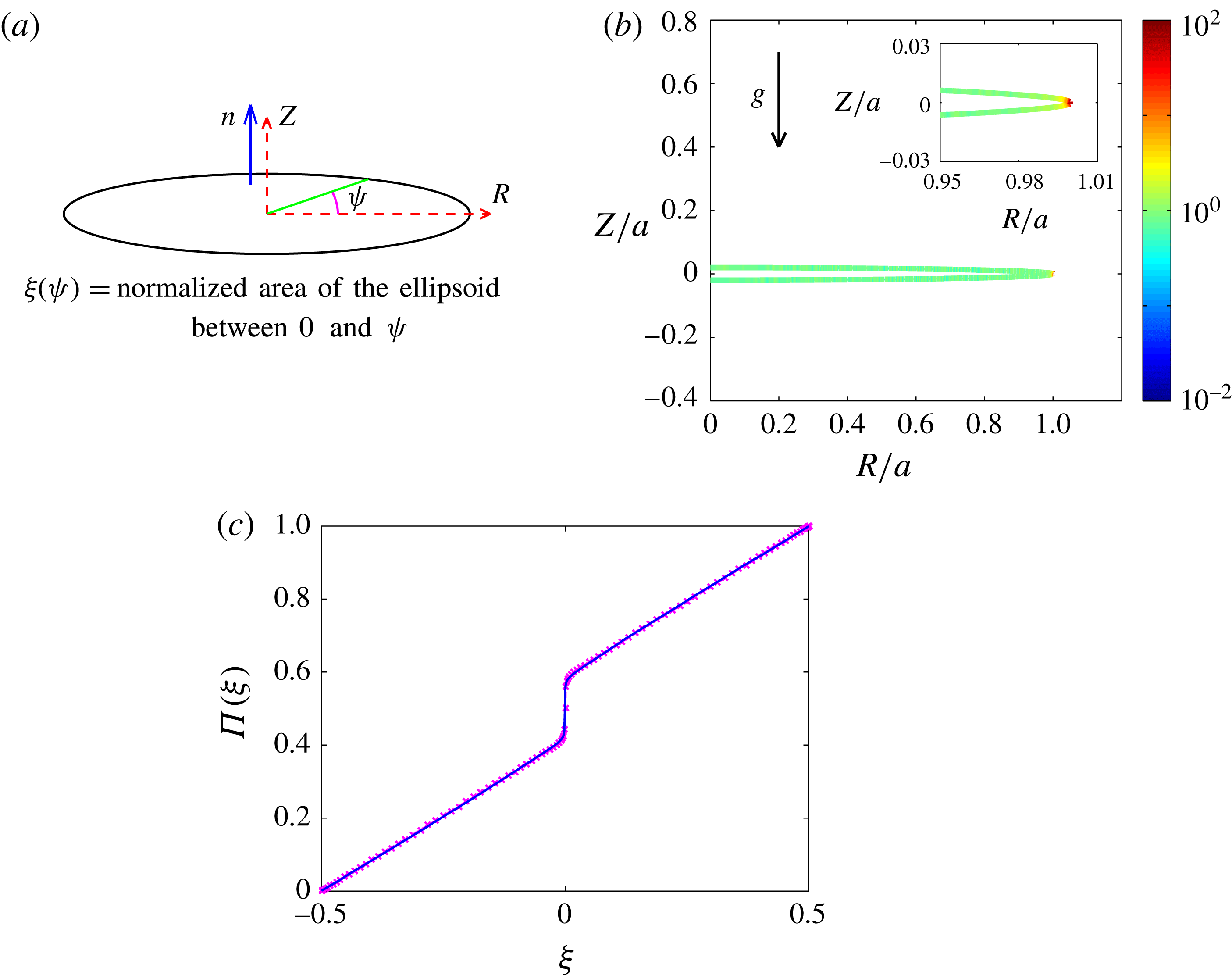
(a) Parametrization of an ellipsoid in a plane containing its shorter axis. The angle
 $\unicode[STIX]{x1D713}$
is related to the angle
 $\unicode[STIX]{x1D719}$
in (6.1) by
 $\unicode[STIX]{x1D713}=\tan ^{-1}(\unicode[STIX]{x1D6FD}\tan (\unicode[STIX]{x1D719}))$
. (b) Representation of the probability of impact of a droplet on the ellipsoid, in the absence of gravity. The colour code is shown on the right. In this case, the probability is approximately uniform, except right on the rim. (c) The cumulative p.d.f. of the location of impact, defined by (6.3), which shows that
 ${\approx}16\,\%$
of all collisions actually occur at the rim. The distribution determined numerically (solid curve) and the theoretical prediction assuming that the centres of the impacting spheres are uniformly distributed on the surface of the extended ellipsoid (‘
 $\times$
’ symbols) perfectly superimpose. Parameters for (b,c):
 $\unicode[STIX]{x1D700}\approx 16~\text{cm}^{2}~\text{s}^{-3}$
,
 $\unicode[STIX]{x1D6FD}=0.02$
,
 $r_{D}=10~\unicode[STIX]{x03BC}\text{m}$
and
 $g=0$
.

To proceed, we begin by introducing the following parametrization of the ellipsoid. A point on the surface of the ellipsoid can be parametrized by two variables. The first one,
 $\unicode[STIX]{x1D719}$
, is defined by writing the distance to the axis of symmetry,
 $R$
, and the vertical distance,
 $Z$
, in the following form:
 $$\begin{eqnarray}R(\unicode[STIX]{x1D719})=a\cos (\unicode[STIX]{x1D719})\quad \text{and}\quad Z(\unicode[STIX]{x1D719})=\unicode[STIX]{x1D6FD}a\sin (\unicode[STIX]{x1D719}).\end{eqnarray}$$
The variable
 $\unicode[STIX]{x1D719}$
in (6.1) is related to the angle
 $\unicode[STIX]{x1D713}$
in figure 7(a) by
 $\unicode[STIX]{x1D713}=\tan ^{-1}(\unicode[STIX]{x1D6FD}\tan (\unicode[STIX]{x1D719}))$
. The second variable is the angle,
 $\unicode[STIX]{x1D703}$
, describing the azimuthal position on the spheroid, with respect to an arbitrary direction in the plane of symmetry. A full representation of the surface of the spheroid is obtained by varying
 $\unicode[STIX]{x1D719}$
in the interval
 $[-\unicode[STIX]{x03C0}/2,\unicode[STIX]{x03C0}/2]$
and
 $\unicode[STIX]{x1D703}$
in the interval
 $[0,2\unicode[STIX]{x03C0})$
. In the present work, we average over the values of
 $\unicode[STIX]{x1D703}$
, so we are only concerned about the probability of impact as a function of
 $\unicode[STIX]{x1D719}$
, over the range
 $-\unicode[STIX]{x03C0}/2\leqslant \unicode[STIX]{x1D719}\leqslant \unicode[STIX]{x03C0}/2$
.
With the elementary parametrization of the ellipsoid given by (6.1), the area on the ellipsoid, between
 $\unicode[STIX]{x1D719}$
and
 $\unicode[STIX]{x1D719}+\text{d}\unicode[STIX]{x1D719}$
, is
 $\text{d}{\mathcal{A}}(\unicode[STIX]{x1D719})=2\unicode[STIX]{x03C0}\,\text{d}s(\unicode[STIX]{x1D719})R(\unicode[STIX]{x1D719})$
, where
 $\text{d}s$
is the arclength along the curve, which leads to
 $$\begin{eqnarray}\text{d}{\mathcal{A}}(\unicode[STIX]{x1D719})=2\unicode[STIX]{x03C0}a^{2}\sqrt{1-(1-\unicode[STIX]{x1D6FD}^{2})\cos ^{2}\unicode[STIX]{x1D719}}\cos \unicode[STIX]{x1D719}\,\text{d}\unicode[STIX]{x1D719}.\end{eqnarray}$$
In the following,
 ${\mathcal{A}}_{tot}={\mathcal{A}}(\unicode[STIX]{x1D719}=\unicode[STIX]{x03C0}/2)-{\mathcal{A}}(\unicode[STIX]{x1D719}=-\unicode[STIX]{x03C0}/2)$
is the total area of the surface of the ellipsoid, and we take the convention that
 ${\mathcal{A}}(\unicode[STIX]{x1D719}=0)=0$
. We use the dimensionless area, defined by dividing
 ${\mathcal{A}}$
by
 ${\mathcal{A}}_{tot}$
:
 $\unicode[STIX]{x1D709}\equiv {\mathcal{A}}/{\mathcal{A}}_{tot}$
. The variable
 $\unicode[STIX]{x1D709}$
is an increasing function of
 $\unicode[STIX]{x1D719}$
, which maps the interval
 $-\unicode[STIX]{x03C0}/2\leqslant \unicode[STIX]{x1D719}\leqslant \unicode[STIX]{x03C0}/2$
onto
 $-1/2\leqslant \unicode[STIX]{x1D709}\leqslant 1/2$
. In what follows, we chose the values of
 $\unicode[STIX]{x1D719}$
and
 $\unicode[STIX]{x1D709}$
in such a way that the direction given by
 $\unicode[STIX]{x1D719}=\unicode[STIX]{x03C0}/2$
(
 $\unicode[STIX]{x1D709}=1/2$
) points upwards, in the direction
 $Z>0$
. In other words, in the presence of gravity, an impact with
 $\unicode[STIX]{x1D709}>0$
(
 $\unicode[STIX]{x1D709}<0$
) is due to a droplet hitting the ellipsoid from above (below).
In the simulations, once the numerical algorithm (see appendix A) has detected that a collision occurs at a given time, we determine, from the positions of the colliding droplet and of the crystal at the collision, the point of contact on the ellipsoid, which we express as a function of the parameters
 $\unicode[STIX]{x1D719}$
and
 $\unicode[STIX]{x1D703}$
, and hence as a function of
 $\unicode[STIX]{x1D709}$
. The position of the impact of the droplets on the surface of the crystal, parametrized by the variable
 $\unicode[STIX]{x1D719}$
, is represented in figure 7(b), for flow 2, with
 $\unicode[STIX]{x1D6FD}=0.02$
and
 $r_{D}=10~\unicode[STIX]{x03BC}\text{m}$
(run 9 of table 3). The probability density function (p.d.f.)
 $P(\unicode[STIX]{x1D709})$
, defined by the condition that the probability of a droplet to impact the ellipsoid between
 $\unicode[STIX]{x1D709}$
and
 $\unicode[STIX]{x1D709}+\text{d}\unicode[STIX]{x1D709}$
is
 $P(\unicode[STIX]{x1D709})\,\text{d}\unicode[STIX]{x1D709}$
, is colour coded, as indicated on the colour bar. The large increase (by almost two orders of magnitude) of
 $P(\unicode[STIX]{x1D709})$
near the rim clearly indicates that the probability of a droplet to impact the ellipsoid at a given position is very far from being uniform (which would have corresponded to a constant value,
 $P(\unicode[STIX]{x1D709})=1$
). The inset in figure 7(b), which blows up in the region very close to the rim, shows that the maximum is very localized. A very quantitative way to characterize this sharp increase of the probability of an impact close to the rim consists in computing the cumulative distribution of impacts,
 $$\begin{eqnarray}\unicode[STIX]{x1D6F1}(\unicode[STIX]{x1D709})=\int _{-1/2}^{\unicode[STIX]{x1D709}}P(\unicode[STIX]{x1D709}^{\prime })\,\text{d}\unicode[STIX]{x1D709}^{\prime }.\end{eqnarray}$$
The values of
 $\unicode[STIX]{x1D6F1}(\unicode[STIX]{x1D709})$
for run 9 (see table 3) are shown in figure 7(c). The dependence of
 $\unicode[STIX]{x1D6F1}$
on
 $\unicode[STIX]{x1D709}$
is essentially linear, except over a very narrow region close to
 $\unicode[STIX]{x1D709}=0$
. The jump of probability over this narrow region is
 ${\approx}0.17$
, the rest of the probabillity being equally split between
 $\unicode[STIX]{x1D709}>0$
and
 $\unicode[STIX]{x1D709}<0$
.
The numerical results summarized in figure 7 therefore show that, in the absence of any gravity or flow anisotropy, the probability of collision is very far from being uniform along the surface of the ellipsoid. This feature can be explained by elementary geometric considerations. A collision occurs when the surface of a droplet hits the surface of the ellipsoid. This happens when the centre of mass of the droplet crosses a surface of the extended ellipsoid, constructed by shifting the points of the ellipsoid of reference, by a distance
 $r_{D}$
, in the direction normal to its surface; see (B 1) of appendix B.
The analysis in appendix B presents the main step of the derivation. As explained in that appendix, we postulate, in an isotropic case (in the absence of settling), that the centre of mass of the droplet hits the point of the extended ellipsoid with a uniform probability. This allows us to explicitly compute the density of impacts along the ellipsoids. The resulting probability, using this geometric construction, is shown as a curve with the ‘
 $\times$
’ symbols in figure 7(c). It is essentially indistinguishable from the probability measured numerically. In particular, it explains the sharp increase of the impact probability near the rim of the ellipsoid.
6.2 Distribution of impacts between settling droplets and ellipsoids
Distribution of the impact point of the droplets on an ellipsoid. (a) Representation of the probability of collision on the surface of the ellipsoid, showing a strong asymmetry between the lower and the upper part of the ellipsoid, and a very strong probability of impact near the rim. (b) Cumulative p.d.f.
 $\unicode[STIX]{x1D6F1}(\unicode[STIX]{x1D709})$
(same convention as in figure 7). The data shown here correspond to
 $r_{D}=10~\unicode[STIX]{x03BC}\text{m}$
,
 $\unicode[STIX]{x1D6FD}=0.02$
and
 $\unicode[STIX]{x1D700}\approx 16~\text{cm}^{2}~\text{s}^{-3}$
(
 $R_{\unicode[STIX]{x1D706}}=95$
).

We investigate now the distribution of the impact point of the droplets on the crystals in the presence of gravitational settling. The parameters chosen in the case of figure 8 correspond to
 $r_{D}=10~\unicode[STIX]{x03BC}\text{m}$
,
 $\unicode[STIX]{x1D6FD}=0.02$
and
 $\unicode[STIX]{x1D700}\approx 16~\text{cm}^{2}~\text{s}^{-3}$
(
 $R_{\unicode[STIX]{x1D706}}=95$
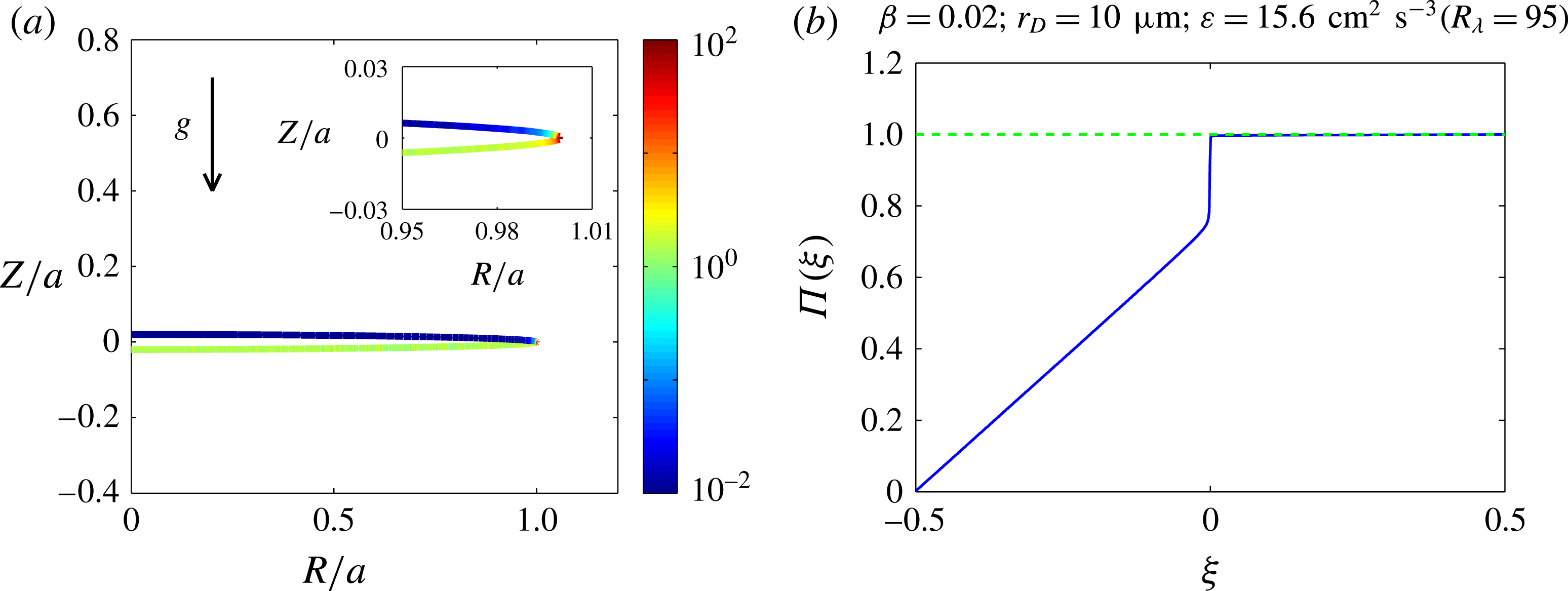
). This corresponds to the case where crystals settle faster than droplets. One clearly sees a strong asymmetry between the upper and the lower parts of the ellipsoids, the latter collecting many more droplets than the former. This is consistent with the expectation that collisions are induced, to a large extent, by the difference in settling velocities between the crystals and the droplets. Asymmetry is clearly visible in all runs with gravity.
As was the case in the absence of gravitational settling, one also observes a strong probability of collision right at the rim. In the representation in terms of the cumulative p.d.f.
 $\unicode[STIX]{x1D6F1}(\unicode[STIX]{x1D709})$
defined by (6.3), the localized peak in probability at the rim can be best measured by the jump in the value of
 $\unicode[STIX]{x1D6F1}$
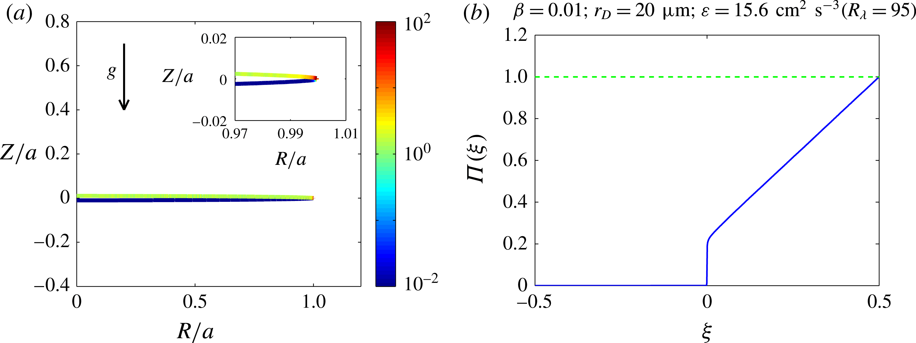
around 0: in the data shown in figure 8, roughly 20 % of all collisions occur at the rim. In sharp contrast with the case without gravity, however (see figure 7), the distribution is very asymmetric: the rest of the collisions happen exclusively on the downward-facing side of the ellipsoids. The same trend is observed, with the notable exception of the run with
 $r_{D}=20~\unicode[STIX]{x03BC}\text{m}$
and
 $\unicode[STIX]{x1D6FD}=0.01$
, where the collisions are occurring mainly on the upward-facing side of the ellipsoid, reflecting the fact that the droplets in this case are settling faster than the crystals; see figure 9.
Distribution of the impact point of the droplets on an ellipsoid in the case where the settling velocity of the droplet exceeds the settling velocity of the ellipsoid (
 $r_{D}=20~\unicode[STIX]{x03BC}\text{m}$
,
 $\unicode[STIX]{x1D6FD}=0.01$
). (a) Representation of the probability of collision on the surface of the ellipsoid, showing a strong asymmetry between the lower and the upper part of the ellipsoid, and a very strong probability of impact near the rim. (b) Cumulative p.d.f.
 $\unicode[STIX]{x1D6F1}(\unicode[STIX]{x1D709})$
(same convention as in figure 7). The data shown here correspond to
 $r_{D}=20~\unicode[STIX]{x03BC}\text{m}$
,
 $\unicode[STIX]{x1D6FD}=0.01$
and
 $\unicode[STIX]{x1D700}\approx 16~\text{cm}^{2}~\text{s}^{-3}$
(
 $R_{\unicode[STIX]{x1D706}}=95$
).

Figures 8 and 9 may suggest that almost no collisions occur on one of the crystal faces. This conclusion is true at the lowest turbulence intensities considered,
 $\unicode[STIX]{x1D700}\approx 1$
and
 $\unicode[STIX]{x1D700}\approx 16~\text{cm}^{2}~\text{s}^{-3}$
. In quantitative terms, no more than 0.3 % of all collisions occur, at
 $\unicode[STIX]{x1D700}\approx 16~\text{cm}^{2}~\text{s}^{-3}$
, on the upward-facing side of the crystal when
 $\unicode[STIX]{x1D6FD}=0.02$
and
 $r_{D}=10~\unicode[STIX]{x03BC}\text{m}$
(corresponding to figure 8). At higher turbulence intensity,
 $\unicode[STIX]{x1D700}\approx 256~\text{cm}^{2}~\text{s}^{-3}$
, this proportion increases to
 ${\approx}3\,\%$
of all collisions. This is a consequence of the increased root-mean-square of the turbulent velocity fluctuations, which is slightly larger than the settling velocity at our highest turbulence intensity (Jucha et al.
Reference Jucha, Naso, Lévêque and Pumir2018). This trend is likely to amplify as the turbulence level grows. In particular, an increase in
 $\unicode[STIX]{x1D700}$
enhances the Stokes number of the droplets (
 $St\propto \unicode[STIX]{x1D700}^{1/2}$
), hence the inertial effects on their motion. This is expected to bring significant changes when the Stokes number of the droplets reaches a value
 $St^{D}\gtrsim 0.3$
(Voßkuhle et al.
Reference Voßkuhle, Pumir, Lévêque and Wilkinson2014). This corresponds to
 $\unicode[STIX]{x1D700}\approx 10\,000~\text{cm}^{2}~\text{s}^{-3}$
for particles of size
 $r_{D}=10~\unicode[STIX]{x03BC}\text{m}$
.
7 Discussion
To model the process of riming, whereby small ice crystals get coated by much smaller droplets in mixed-phase clouds, we have considered the simplified problem of collisions between narrow oblate ellipsoids with much smaller spherical droplets in a homogeneous, isotropic turbulent flow. The range of parameters chosen in this work was inspired by the physical conditions present in mixed-phase clouds, at
 $T=-20\,^{\circ }\text{C}$
. The collision rate has been determined over a range of values of droplet radius,
 $r_{D}$
(
 $5~\unicode[STIX]{x03BC}\text{m}\leqslant r_{D}\leqslant 20~\unicode[STIX]{x03BC}\text{m}$
), of the rate of dissipation of kinetic energy per unit volume,
 $\unicode[STIX]{x1D700}$
(
 $1~\text{cm}^{2}~\text{s}^{-3}\lesssim \unicode[STIX]{x1D700}\lesssim 256~\text{cm}^{2}~\text{s}^{-3}$
), and of the aspect ratio of the crystals or, equivalently, of their mass,
 $\unicode[STIX]{x1D6FD}$
(
 $0.01\leqslant \unicode[STIX]{x1D6FD}\leqslant 0.05$
).
In order to disentangle the role of the two main effects, differential settling and turbulence, we have also considered the problem in the absence of gravity, although this is clearly an unrealistic approximation in the cloud context.
The model clearly involves a number of simplifications. First, we are merely assuming that the flow is strictly homogeneous, isotropic and turbulent. While a general expectation is that the small-scale properties of any flow at large enough Reynolds number should be homogeneous and isotropic (Kolmogorov Reference Kolmogorov1941), the flows considered in this work are certainly not in this regime, so the effects of the large-scale flow could affect the small-scale properties, hence the collision rates discussed here. Second, the description of the motion of the crystals rests on a set of rational, although not fully tested, approximations. The possible shortcomings of the model, due in particular to possible corrections that result from the effect of fluid inertia (Leal Reference Leal1980; Candelier, Einarsson & Mehlig Reference Candelier, Einarsson and Mehlig2016) and discussed elsewhere, in particular in Jucha et al. (Reference Jucha, Naso, Lévêque and Pumir2018), need to be further explored and quantified.
In this work, we merely determined when the surfaces of a sphere and of an ellipsoid touch. The modification of the flow when the two particles get close to each other is not taken into account. Last, in our calculations, the particles do not aggregate, and continue further their paths (ghost-collision approximation).
Numerically, we have followed a large set of droplets and crystals, and determined the collision rate using the ghost-collision approximation. In the presence of gravitational settling, our numerical results indicate that the collision rate can be parametrized, at least in the range of parameters considered, with a turbulent enhancement factor
 $E_{DC}\approx 0.3{-}0.4$
, provided the crystals settle faster than the droplets. In the case of larger droplets and thinner crystals, we observed that droplets may settle faster than crystals. In this case, the limited information provided by our study indicates that the turbulent enhancement factor is significantly larger (
 $E_{DC}\approx 1.8$
).
Over the range of parameters considered, our results indicate that the collision rate is significantly weaker in the absence of any gravitational settling. The collision rate in the absence of gravity, however, very significantly increases with the turbulence intensity (the rate of energy dissipation per unit volume,
 $\unicode[STIX]{x1D700}$
), faster than one would expect based on elementary considerations (Saffman & Turner Reference Saffman and Turner1956). As a result, in very turbulent clouds, assuming that collisions are due merely to differential settling may underestimate the collision rate. A simplistic extrapolation of our results suggests that this may happen when
 $\unicode[STIX]{x1D700}\gtrsim 1000~\text{cm}^{2}~\text{s}^{-3}$
.
In all cases, we detected that collisions occur with a very large probability at the rim of the crystals (with the parameters we used, 10 %–20 % of all collisions occur right at the rim). This can be explained by very elementary geometric considerations. Crystals settling in a gravitational field collide with droplets exclusively on the downward-facing (respectively, upward-facing) side of the crystals, when the crystal settles faster (respectively, slower) than the droplets, with a finite fraction happening in a very small neighbourhood around the rim. This conclusion needs to be revisited in the case of a very turbulent cloud.
The present study suggests a number of further investigations. Determining the statistics of the translational and orientational degrees of freedom of the crystals after their collisions with droplets, under various assumptions on the nature of the collision (elastic or inelastic) should provide interesting hints on the outcome of collisions. It would also be interesting to carry out similar investigations at higher Reynolds numbers. In these regimes, we expect that the more intense fluctuations of the velocity gradients would modify the statistical properties of the crystals’ orientation, and would lead to stronger inertial effects for the droplets, leading to clustering, or to the formation of caustics (Pumir & Wilkinson Reference Pumir and Wilkinson2016), potentially leading to enhanced collision rates. Increasing the role of the droplets’ inertia could be alternatively achieved by considering larger values of
 $r_{D}$
, which would conceivably result in a significant enhancement of the collision rate. Finally, varying the crystals’ aspect ratio simultaneously with their size so as to keep the mass constant could lead to interesting new insight.
Although obtained with a set of simplifying approximations, our results provide important information on the collision rates between ice crystals and water droplets in clouds, as well as on the physical mechanisms that affect these rates. As such, our work is expected to provide useful insights that should be incorporated in more realistic models of riming.
Acknowledgements
We are grateful to S. Borrmann, K. Gustavsson, S. Malinowski, B. Mehlig, R. Shaw and C. Siewert for many discussions and insights at various stages of this work. The simulations have been performed by using the local HPC facilities at ENS de Lyon (PSMN) and at the Université Lyon-I (P2CHPD) mainly supported by the Auvergne-Rhône-Alpes region (Grant CPRT07-13 CIRA) and the project Equip@Meso (ANR-10-EQPX-29-01). A.N., E.L. and A.P. have been supported by the grant ‘TEC’ 2 from ANR (ANR-12-BS09-0011-02), and by the EU COST action MP0806 ‘Particles in Turbulence’. J.J. and A.P. acknowledge the support from the Alexander-von-Humboldt Foundation. A.P. is also very grateful to the visitor programme of the Max-Planck-Institute for Dynamics and Self-Organisation in Göttingen, Germany.
Appendix A. Numerical detection of collisions
The algorithm of detection used was first implemented in a similar context by Siewert et al. (Reference Siewert, Kunnen, Meinke and Schröder2014a
). We are considering here collisions, determined geometrically by the contact between two surfaces, which are both described by polynomial equations of second order. Namely, we write the equations of the two surfaces in the form
 $\boldsymbol{X}^{\text{T}}\boldsymbol{\cdot }\unicode[STIX]{x1D63C}_{e,d}\boldsymbol{\cdot }\boldsymbol{X}=0$
, where
 $\boldsymbol{X}$
is a vector with four real components, defined by
 $\boldsymbol{X}^{\text{T}}=(x,y,z,1)$
, and
 $\unicode[STIX]{x1D63C}_{e,d}$
are two
 $4\times 4$
matrices parametrizing them. The polynomial of the real variable
 $\unicode[STIX]{x1D701}$
, defined by
 $$\begin{eqnarray}\overline{P}(\unicode[STIX]{x1D701})\equiv \det (\unicode[STIX]{x1D63C}_{e}-\unicode[STIX]{x1D701}\unicode[STIX]{x1D63C}_{d}),\end{eqnarray}$$
always has two positive real roots (Choi et al.
Reference Choi, Chang, Wang, Kim and Elber2009). In the case where the two surfaces are separated and do not overlap, the other two roots of
 $\overline{P}$
are real and negative, whereas they are imaginary when the two surfaces overlap. When the two surfaces are in contact,
 $\overline{P}$
has a real negative double root.
Here, we are interested in ellipsoids and droplets moving in space. This implies that, for each pair of an ellipsoid and a droplet, the polynomial
 $\overline{P}$
also depends on time. The condition of contact is therefore that, at a given time
 $t$
, the polynomial
 $\overline{P}(\unicode[STIX]{x1D701},t)$
has a double negative root.
This condition can be implemented as proposed by Siewert et al. (Reference Siewert, Kunnen, Meinke and Schröder2014a
). Namely, we construct an approximation of the function
 $\overline{P}(\unicode[STIX]{x1D701},\unicode[STIX]{x1D70F})$
between two consecutive time steps,
 $t\leqslant \unicode[STIX]{x1D70F}\leqslant t+\unicode[STIX]{x0394}t$
, which is polynomial in
 $\unicode[STIX]{x1D70F}$
. To construct the dependence on
 $\unicode[STIX]{x1D70F}$
, we assume that the centres of mass move with a uniform velocity between the two time steps, and we neglect the rotation of the ellipsoid, which allows us to keep only a third-order polynomial dependence on
 $\unicode[STIX]{x1D70F}$
. Taking into account the rotation of the ellipsoid between
 $t$
and
 $t+\unicode[STIX]{x0394}t$
would lead to a much higher polynomial approximation (of order 48). The accurate determination of the roots of the polynomials studied is a crucial step in the algorithm. Effectively, this constraint makes it impracticable to work with too high a polynomial order; for this reason, we neglect the rotation of the ellipsoid between two time steps. With the resulting polynomials of degrees four in
 $\unicode[STIX]{x1D701}$
and three in
 $\unicode[STIX]{x1D70F}$
, we looked systematically for configurations where the polynomial switches from two negative roots (before the collision) to a negative double root (right at the collision time) in
 $\unicode[STIX]{x1D701}$
.
To reduce the otherwise prohibitive effort of considering all pairs of ellipsoids and spheres, we restricted the search by partitioning space, as proposed, for example, in Sundaram & Collins (Reference Sundaram and Collins1996) and Siewert et al. (Reference Siewert, Kunnen, Meinke and Schröder2014a ).
Appendix B. Geometric determination of the probability of impact along the crystal in the absence of gravity
This appendix contains the key elements in the derivation of the probability of impacts along the surface of the ellipsoid in the absence of gravity or of any flow anisotropy, shown in figure 7(c) in § 6.1. The construction is based on two observations.
First, when a droplet hits the ellipsoid at a point parametrized by the angle
 $\hat{\unicode[STIX]{x1D719}}$
, as defined by (6.1), its centre of mass crosses the surface parametrized by
 $$\begin{eqnarray}\displaystyle \left.\begin{array}{@{}c@{}}R_{+}(\unicode[STIX]{x1D719})=\cos (\unicode[STIX]{x1D719})\left[a+{\displaystyle \frac{\unicode[STIX]{x1D6FD}r_{D}}{\sqrt{1-(1-\unicode[STIX]{x1D6FD}^{2})\cos (\unicode[STIX]{x1D719})^{2}}}}\right]\!,\\ Z_{+}(\unicode[STIX]{x1D719})=\sin (\unicode[STIX]{x1D719})\left[\unicode[STIX]{x1D6FD}a+{\displaystyle \frac{r_{D}}{\sqrt{1-(1-\unicode[STIX]{x1D6FD}^{2})\cos (\unicode[STIX]{x1D719})^{2}}}}\right]\!,\end{array}\right\} & & \displaystyle\end{eqnarray}$$
at the angle
 $\unicode[STIX]{x1D719}=\hat{\unicode[STIX]{x1D719}}$
. In what follows, we refer to the surface parametrized by (B 1) as the extended ellipsoid.
Second, in the case of an isotropic flow (in the absence of settling), we make the plausible assumption that droplets colliding with the ellipsoid, with a centre of mass initially outside the extended ellipsoid, come from all spatial directions, and all origins with equal probability. Our assumption is directly inspired by standard arguments from the kinetic theory of gases, such as those used to compute pressure (Huang Reference Huang1987). The centres of mass of the colliding droplets are therefore hitting each element of the extended ellipsoid, defined by (B 1), with a uniform probability per area. Specifically, we assume that, in the case of an isotropic flow, the velocity of the centres of mass of the droplets are distributed isotropically, with a p.d.f.
 ${\mathcal{P}}(v)$
of the norm of their velocities. An elementary calculation shows that the number of particles hitting an area
 $\text{d}{\mathcal{A}}_{+}$
along the extended ellipsoid per unit mass is simply
 $2\unicode[STIX]{x03C0}n_{0}(\int _{0}^{\infty }{\mathcal{P}}(v)v\,\text{d}v)$
, where
 $n_{0}$
is the number of droplets per unit volume, assumed to be constant.
Under these two assumptions, the probability that a droplet collides with the ellipsoid at a position corresponding to an angle between
 $\unicode[STIX]{x1D719}$
and
 $\unicode[STIX]{x1D719}+\text{d}\unicode[STIX]{x1D719}$
is simply proportional to the area of the extended ellipsoid, parametrized by (B 1), between
 $\unicode[STIX]{x1D719}$
and
 $\unicode[STIX]{x1D719}+\text{d}\unicode[STIX]{x1D719}$
. This area is simply
 $\text{d}{\mathcal{A}}_{+}=2\unicode[STIX]{x03C0}R_{+}(\unicode[STIX]{x1D719})\,\text{d}s_{+}(\unicode[STIX]{x1D719})$
, where
 $(\text{d}s_{+}/\text{d}\unicode[STIX]{x1D719})^{2}=(\text{d}R_{+}/\text{d}\unicode[STIX]{x1D719})^{2}+(\text{d}Z_{+}/\text{d}\unicode[STIX]{x1D719})^{2}$
. A simple calculation shows that
 $$\begin{eqnarray}\displaystyle \text{d}{\mathcal{A}}_{+} & = & \displaystyle \text{d}{\mathcal{A}}\times \left(1+\frac{\unicode[STIX]{x1D6FD}r_{D}}{a}\frac{1}{[1-(1-\unicode[STIX]{x1D6FD}^{2})\cos (\unicode[STIX]{x1D719})^{2}]^{3/2}}\right)\nonumber\\ \displaystyle & & \displaystyle \times \,\left(1+\frac{\unicode[STIX]{x1D6FD}r_{D}}{a}\frac{1}{[1-(1-\unicode[STIX]{x1D6FD}^{2})\cos (\unicode[STIX]{x1D719})^{2}]^{1/2}}\right),\end{eqnarray}$$
where
 $\text{d}{\mathcal{A}}$
is the area of the original ellipsoid, given by (6.2).
Given that the number of impacts per unit area of the extended ellipsoid is constant, the ratio
 $\text{d}{\mathcal{A}}_{+}/\text{d}{\mathcal{A}}$
is proportional to the probability of impact on the surface of the original ellipsoid.
The small values of
 $\unicode[STIX]{x1D6FD}$
and of
 $r_{D}/a$
chosen here, both
 ${\approx}10^{-2}$
, make the ratio
 $\text{d}{\mathcal{A}}_{+}/\text{d}{\mathcal{A}}\approx 1$
, except when
 $\cos (\unicode[STIX]{x1D719})\approx 1$
, i.e. close to the rim. For
 $\unicode[STIX]{x1D719}\approx 0$
, we expand
 $\cos (\unicode[STIX]{x1D719})^{2}\approx 1-\unicode[STIX]{x1D719}^{2}$
to obtain the limiting form
 $$\begin{eqnarray}\text{d}{\mathcal{A}}_{+}/\text{d}{\mathcal{A}}\approx \left[1+\frac{\unicode[STIX]{x1D6FD}r_{D}}{a}\frac{1}{(\unicode[STIX]{x1D719}^{2}+\unicode[STIX]{x1D6FD}^{2})^{1/2}}\right]\left[1+\frac{\unicode[STIX]{x1D6FD}r_{D}}{a}\frac{1}{(\unicode[STIX]{x1D719}^{2}+\unicode[STIX]{x1D6FD}^{2})^{3/2}}\right].\end{eqnarray}$$
The first term in brackets on the right-hand side of (B 3) has maximum
 $1+(r_{D}/a)$
when
 $\unicode[STIX]{x1D719}\rightarrow 0$
, which is very close to
 $1$
. The maximum of the second term in brackets is of the order
 $1+(r_{D}/a)/\unicode[STIX]{x1D6FD}^{2}$
when
 $\unicode[STIX]{x1D719}\rightarrow 0$
, which is much larger than 1, therefore explaining the large increase of the probability near the rim. The increase of the probability near the rim is limited to values of
 $\unicode[STIX]{x1D719}\approx \unicode[STIX]{x1D6FD}$
. The total contribution due to the rim,
 $\int _{\unicode[STIX]{x1D719}\approx 0}\text{d}{\mathcal{A}}_{+}$
, is of order
 $(r_{D}/a)(1/\unicode[STIX]{x1D6FD})$
, which is finite, and of order 1 for the values chosen here, consistent with the observation of figure 7(c).
The main qualitative content of equations (B 3) which justifies the strong increase of the probability of collisions near the edges of the ellipsoid can be understood in qualitative terms by noting that the arclength
 $\text{d}s$
between
 $\unicode[STIX]{x1D719}$
and
 $\unicode[STIX]{x1D719}+\text{d}\unicode[STIX]{x1D719}$
along the original ellipsoid becomes, on the extended one,
 $\text{d}s_{+}=\text{d}s(1+a/r_{c})$
, where
 $r_{c}$
is the radius of curvature of the ellipsoid. The sharp decrease of the radius of curvature at the edge of the original (non-extended) ellipsoid explains the effect observed in figure 7(c).