



1 Introduction
The Hausdorff and box dimensions are the most common notions to quantify the size of sets in fractal geometry; see [Reference Falconer15, Reference Mattila31] for an introduction. It is natural to ask under which condition these two dimensions coincide, especially for invariant sets in dynamical systems. This is an important question and has a long history. Furstenberg [Reference Furstenberg20] showed that if
 $ K $
is a compact set invariant under an expanding conformal endomorphism on the d-torus, then
 $$ \begin{align} \dim_{\mathrm{H}} K = \dim_{\mathrm{B}} K, \end{align} $$
where
 $ \dim _{\mathrm {H}} $
and
 $ \dim _{\mathrm {B}} $
stand for the Hausdorff and box dimensions, respectively. Subsequently, (A) has been proved to hold in various conformal settings [Reference Barreira3, Reference Falconer13, Reference Gatzouras and Peres22] and some typical non-conformal settings [Reference Falconer12, Reference Käenmäki and Vilppolainen24]. Notably, Falconer proved that (A) holds for all self-similar sets [Reference Falconer13] and certain typical self-affine sets [Reference Falconer12]. In contrast, the Hausdorff and box dimensions are usually distinct in specific non-conformal settings. In this paper, we study when (A) holds for the invariant sets in the following family of non-conformal dynamical systems. Let
 $ T $
be an expanding linear endomorphism on the
 $ d $
-torus
 $ \mathbb {T}^{d} = \mathbb {R}^{d}/\mathbb {Z}^{d} $
represented by a diagonal integer matrix
 $$ \begin{align*} \Lambda = \operatorname{\mathrm{diag}} (m_{1}, \ldots, m_{d}), \end{align*} $$
where
 $ m_{1} \geq \cdots \geq m_{d} \geq 2 $
, that is,
 $ T(x) = \Lambda x \,\mod 1 $
for
 $ x \in [0,1)^{d}$
. Write the number of distinct expanding ratios as
 $$ \begin{align} s = \# \{m_{i}: 1 \leq i \leq d\} , \end{align} $$
where
 $\# $
stands for cardinality. Let
 $ \mathcal {A} = \prod _{j=1}^{d} \{ 0, \ldots , m_{j} - 1 \} $
. There is a canonical representation map
 $ R \colon \mathcal {A}^{\mathbb {N}} \to \mathbb {T}^{d} $
given by
 $$ \begin{align} R(x) = \sum_{k=1}^{\infty} \Lambda^{-k} x_{k} \quad \text{for } x = (x_{k})_{k=1}^{\infty} \in \mathcal{A}^{\mathbb{N}}. \end{align} $$
Let
 $ \sigma $
be the (left) shift on
 $\mathcal {A}^{\mathbb {N}}$
defined as
 $ \sigma ((x_{k})_{k=1}^{\infty } ) = (x_{k+1})_{k=1}^{\infty } $
. Endow
 $ \mathcal {A}^{\mathbb {N}} $
with the product topology. A closed subset
 $ X $
of
 $ \mathcal {A}^{\mathbb {N}}$
is called a subshift if
 $\sigma (X) \subset X $
. Since
 $ R $
is a continuous surjective map and
 $ R\circ \sigma = T \circ R $
, there is a one-to-one correspondence between the subshifts of
 $ \mathcal {A}^{\mathbb {N}}$
and the compact T-invariant subsets of
 $ \mathbb {T}^{d}$
. When
 $ {K = R(\mathcal {D}^{\mathbb {N}})} $
for some non-empty subset
 $ \mathcal {D} $
of
 $ \mathcal {A}$
, we call K a Bedford–McMullen carpet if
 $ d = 2$
and a Bedford–McMullen sponge if
 $ d \geq 3 $
.
Given a continuous increasing function
 $ \varphi \colon [0, \infty ) \to [0, \infty ) $
with
 $ \varphi (0) = 0 $
, called a gauge function, for
 $ E \subset \mathbb {R}^{d} $
and
 $ \delta> 0 $
, define
 $$ \begin{align*} \mathcal{H}_{\delta}^{\varphi}(E) = \inf \bigg \{\kern-3pt \sum_{i=1}^{\infty} \varphi(\lvert E_{i}\rvert) \colon \{E_{i}\}_{i=1}^{\infty} \text{ is a cover of } E \text{ and } \lvert E_{i}\rvert \leq \delta \text{ for all } i \bigg \}, \end{align*} $$
where
 $ \lvert F\rvert $
denotes the diameter of a set
 $ F \subset \mathbb {R}^{d} $
in Euclidean norm. The Hausdorff measure of
 $ E $
is
 $$ \begin{align*} \mathcal{H}^{\varphi}(E) = \lim_{\delta\to 0} \mathcal{H}_{\delta}^{\varphi}(E). \end{align*} $$
Write
 $ \mathcal {H}_{\delta }^{\varphi }$
as
 $ \mathcal {H}_{\delta }^{\gamma }$
and
 $ \mathcal {H}^{\varphi } $
as
 $ \mathcal {H}^{\gamma } $
if
 $ \varphi (t) = t^{\gamma }$
for some
 $\gamma \geq 0 $
. We say that there exists a gauge function for
 $ K \subset \mathbb {R}^{d}$
if
 $$ \begin{align} 0 < \mathcal{H}^{\varphi}(K) < \infty \quad\text{for } \text{some gauge function } \varphi. \end{align} $$
In this paper, for a compact T-invariant set
 $ K $
, we aim to characterize the coincidence of dimensions as in (A) by the existence of gauge functions as in (B).
Our research target is motivated as follows. In the 1980s, Bedford [Reference Bedford4] and McMullen [Reference McMullen32] independently computed the Hausdorff and box dimensions of Bedford–McMullen carpets. Later, their work was extended by Kenyon and Peres [Reference Kenyon and Peres25, Reference Kenyon and Peres26] to Bedford–McMullen sponges and certain sofic affine-invariant sets; see [Reference Barański1, Reference Feng and Wang18, Reference Fraser19, Reference Lalley and Gatzouras29] for some other generalizations. For a Bedford–McMullen carpet K, McMullen [Reference McMullen32] pointed out that
 $ 0 < \mathcal {H}^{\dim _{\mathrm {H}} K}(K) < \infty $
if
 $\dim _{\mathrm {H}} K = \dim _{\mathrm {B}} K $
, and asked about the value of
 $\mathcal {H}^{\dim _{\mathrm {H}} K}(K)$
when
 $ \dim _{\mathrm {H}} K < \dim _{\mathrm {B}} K $
. This question was answered by Peres [Reference Peres37] who proved that
 $ \mathcal {H}^{\dim _{\mathrm {H}} K}(K) = \infty $
if
 $ \dim _{\mathrm {H}} K < \dim _{\mathrm {B}} K $
. Afterwards, Peres [Reference Peres36] showed that if
 $ \dim _{\mathrm {H}} K < \dim _{\mathrm {B}} K $
, the packing measure of K at its packing dimension (which coincides with
 $ \dim _{\mathrm {B}} K $
, see e.g. [Reference Falconer15, Corollary 3.10]) is also infinite. Before the result of Peres [Reference Peres37], an elegant argument found independently by Bedford and Mandelbrot (unpublished) and by Gatzouras and Lalley [Reference Lalley and Gatzouras29] gives the equivalence of (A) and (B) for Bedford–McMullen carpets (see e.g. [Reference Peres37, Proposition 2]). Actually, Gatzouras and Lalley [Reference Lalley and Gatzouras29] showed that
 $ \dim _{\mathrm {H}} K = \dim _{\mathrm {B}} K $
is equivalent to
 $ 0 < \mathcal {H}^{\dim _{\mathrm {H}} K}(K) < \infty $
for a Gatzouras–Lalley carpet
 $ K $
which is a generalization of a Bedford–McMullen carpet by relaxing the grid structure but keeping the dominated directions. These previous results motivate us to study the equivalence of (A) and (B) for invariant subsets of Bedford–McMullen sponges (also called sub-self-affine sets [Reference Falconer14, Reference Käenmäki and Vilppolainen24]).
To state our results, we introduce another related condition that the Hausdorff dimension of the measure of maximal entropy attains the Hausdorff dimension of its support. For a subshift
 $ X $
of
 $ \mathcal {A}^{\mathbb {N}} $
, write
 $$ \begin{align*} \mathcal{L}_{k}(X_{}) = \{ i_{1} \cdots i_{k} \in \mathcal{A}^{k} \colon i_{1}\cdots i_{k} = x_{1}\cdots x_{k} \text{ for some } (x_{j})_{j=1}^{\infty} \in X \}, \quad k \in \mathbb{N}, \end{align*} $$
and
 $$ \begin{align*} {\mathcal{L}(X)} = \operatorname*{\mathrm{\bigcup}}_{k=1}^{\infty} \mathcal{L}_{k}(X_{}) \cup \{\varnothing\}, \end{align*} $$
where
 $ \varnothing $
denotes the empty word. For
 $ I \in \mathcal {A}^{k}$
, denote
 $ \lvert I\rvert = k $
. Set
 $ \lvert \varnothing \rvert = 0 $
. Let
 $ IJ $
denote the juxtaposition of
 $ I, J \in \mathcal {L}(X)$
. We say a subshift
 $ X $
satisfies weak specification if there exists an integer
 $ p $
such that for every
 $ I, J \in \mathcal {L}(X) $
, there is
 $ W \in \mathcal {L}(X) $
with
 $ \lvert W\rvert \leq p $
such that
 $ IWJ \in \mathcal {L}(X) $
. The concept of specification traces back to the seminal work of Bowen [Reference Bowen5, Reference Bowen6] on the uniqueness of equilibrium states (see [Reference Climenhaga and Thompson8]), and plays a key role in the existence of the box dimension of
 $ R(X) $
(see Proposition 3.3 and [Reference Jurga23]). Let
 $ X $
be a subshift satisfying weak specification and
 $ K = R(X)$
. There is a unique
 $\sigma $
-invariant measure of maximal entropy
 $ \mu $
on
 $ X $
(see Proposition 2.2). Then, we give another condition that
 $$ \begin{align} \dim_{\mathrm{H}} R\mu = \dim_{\mathrm{H}} K, \end{align} $$
where
 $ R\mu = \mu \circ R^{-1} $
is the push-forward of
 $ \mu $
under
 $ R $
, and
 $ \dim _{\mathrm {H}} R\mu $
is the Hausdorff dimension of
 $ R\mu $
defined to be the infimum of the Hausdorff dimension of Borel sets with positive
 $R\mu $
-measure.
Now, we are ready to state our first result.
Theorem 1.1. Let
 $ X $
be a subshift satisfying weak specification and
 $ K = R(X) $
. Recall the definition of
 $ s $
from (1.1). Then, the following statements hold:


In [Reference Peres37, p. 526], Peres conjectured that when
 $d = 2$
and
 $ K = R(X) $
, where
 $ X $
is a primitive subshift of finite type,
 $ \mathcal {H}^{\dim _{\mathrm {H}} K}(K) = \infty $
if
 $ \dim _{\mathrm {H}} K < \dim _{\mathrm {B}} K $
. Since such X satisfies weak specification, it follows from Theorem 1.1(iii) that
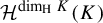 $ \mathcal {H}^{\dim _{\mathrm {H}} K }(K) $
is either
 $ 0 $
or
 $ \infty $
if
 $ \dim _{\mathrm {H}} K < \dim _{\mathrm {B}} K$
.
Let us give some ideas about the proof of Theorem 1.1. First, we characterize (A) in terms of the size of the fibers of certain factor maps; see Theorem 3.1(c), which is by adapting and extending some arguments of [Reference Kenyon and Peres25] to the setting of weak specification. Based on this characterization and the Gibbs property of the measure of maximal entropy, we obtain an upper bound on the density of
 $R\mu $
, leading to the part of statement (i) that
 $\mathcal {H}^{\dim _{\mathrm {H}} K}(K)> 0 $
. Unlike Bedford–McMullen carpets corresponding to the full shifts, in the case of subshifts, it is difficult to estimate the density of
 $ R\mu $
from below. Instead of following the approach based on the density to prove the other part of statement (i) that
 $ \mathcal {H}^{\dim _{\mathrm {H}} K}(K) < \infty $
, we directly consider the covers consisting of the approximate cubes whose number is estimated using weak specification. The proof of statement (ii) is based on the translation-invariance of Hausdorff measures and the Gibbs property of the measure of maximal entropy; see Proposition 5.2. Next, we move to the proof of statement (iii) which is more difficult and requires new ideas since the Hausdorff dimension of T-invariant sets is expressed as a certain topological pressure instead of the simple formula for Bedford–McMullen carpets. By statements (i) and (ii), it suffices to show that (C) implies (A) when
 $ s \leq 2 $
; see Lemma 5.3. To this end, we manage to compute the Hausdorff dimension of the invariant set based on the key observation that the projection of the measure of full dimension to the weakest unstable direction always has the Gibbs property. As for statement (iv), we give some examples of Bedford–McMullen sponges (Examples 7.1 and 7.2) with the desired properties, which is a new phenomenon not appearing in the planar cases.
To determine the Hausdorff measures of Examples 7.1 and 7.2, we manage to give a sufficient condition for Bedford–McMullen sponges to have infinite Hausdorff measures (see Proposition 6.6), and conclude that Examples 7.1 and 7.2 have infinite Hausdorff measures at their respective Hausdorff dimensions. The proof of Proposition 6.6 is based on the method of Peres [Reference Peres37] (see Proposition 6.5) and a newfound relation satisfied by the measure of full dimension (see Lemma 6.8). It is worth pointing out that in [Reference Peres37, §5], Peres mentioned the result [Reference Peres37, Theorem 1] that
 $\mathcal {H}^{\dim _{\mathrm {H}} K}(K) = \infty $
if
 $\dim _{\mathrm {H}} K < \dim _{\mathrm {B}} K $
for a Bedford–McMullen carpet
 $ K $
can extend to Bedford–McMullen sponges. However, he did not give a detailed justification.
The equivalence of (A) and (B) may still hold when
 $ s \geq 3 $
. However, statement (iv) shows that our current strategy for the proof of statement (iii) cannot extend to
 $ s \geq 3 $
. Nevertheless, through a different probabilistic approach, we obtain the equivalence of (A) and (B) for Bedford–McMullen sponges.
The proof of Theorem 1.2 is based on the independence of the coordinates of a random sequence whose law is a Bernoulli measure on
 $\mathcal {A}^{\mathbb {N}}$
and the density theorem for the Hausdorff measures. To the best of our knowledge, the previous known proofs for the equivalence of (A) and (B) for Bedford–McMullen carpets essentially rely on the equivalence of (A) and (C) (see e.g. [Reference Peres37, Proposition 2]), which does not work for Bedford–McMullen sponges as seen in Example 7.1. We remark that a similar proof of Theorem 1.2 based on the density theorem for the packing measures shows that for a Bedford–McMullen sponge
 $ K$
,
 $\dim _{\mathrm {H}} K = \dim _{\mathrm {B}} K $
is equivalent to that, with respect to some (doubling) gauge function
 $ \varphi $
, the packing measure of
 $ K $
is positive and finite. One may expect that Theorem 1.2 can extend to some subshifts if the limit theorem used in the proof of Theorem 1.2 holds under some weaker independence; see Remark 6.4 for an illustration.
The paper is organized as follows. In §2, we make some preparations for the proofs of the main theorems. In §3, we extend the results in [Reference Kenyon and Peres25] to the setting of weak specification. Section 4 is for the proof of Theorem 1.1(i). The proofs of Theorem 1.1(ii) and (iii) are given in §5. Section 6 is devoted to the results about Bedford–McMullen sponges including the proof of Theorem 1.2. The examples for Theorem 1.1(iv) are given in §7.
2 Preliminaries
In §2.1, we introduce the subshifts and factor maps. Then, we present some results about the measures of maximal entropy and full dimension respectively in §§2.2 and 2.3. The last subsection is devoted to the approximate cubes and the related results.
Throughout this paper, we shall mean by
 $ a \lesssim b $
that
 $ a \leq Cb $
for some positive constant
 $ C $
, and write
 $ a \approx b $
if
 $ a \lesssim b $
and
 $ b \lesssim a $
.
2.1 Subshift and factor map
Let
 $\mathcal {B}$
be a finite set. Let
 $ k \in \mathbb {N} $
and
 $ 0 \leq a < b \leq k $
. For
 $ x = (x_{i})_{i=1}^{\infty } \in \mathcal {B}^{\mathbb {N}}$
, write
 $ x|_{a}^{b} = x_{a+1} \cdots x_{b}$
and
 $ x|k = x_{1}\cdots x_{k} $
. By convention, we set
 $ x|0 = \varnothing $
and
 $\lvert \varnothing \rvert = 0 $
, where
 $\varnothing $
denotes the empty word. For
 $ I = i_{1}\cdots i_{k} \in \mathcal {B}^{k} $
, define
 $ I|_{a}^{b} = i_{a+1}\cdots i_{b}$
,
 $ \lvert I\rvert = k $
, and
 $ [I] = \{ x \in \mathcal {B}^{\mathbb {N}} \colon x|k = I \}$
. For
 $ I \in \mathcal {B}^{k_{1}}$
and
 $ J \in \mathcal {B}^{k_{2}}$
, let
 $ IJ $
denote the juxtaposition of
 $ I$
and J. Endow
 $\mathcal {B}^{\mathbb {N}}$
with the product topology. Let
 $ \sigma $
be the shift on
 $\mathcal {B}^{\mathbb {N}}$
defined by
 $ \sigma ( (x_{k})_{k=1}^{\infty } ) = (x_{k+1})_{k=1}^{\infty } $
. A closed subset
 $ X $
of
 $\mathcal {B}^{\mathbb {N}}$
is called a subshift of
 $ \mathcal {B}^{\mathbb {N}}$
if
 $\sigma (X) \subset X $
. Let
 $ \mathcal {M}_{\sigma }(X) $
denote the set of
 $\sigma $
-invariant probability measures on
 $ X $
. Define
 $$ \begin{align*} \mathcal{L}_{k}(X_{}) = \{ I \in \mathcal{B}^{k} \colon [I] \operatorname*{\mathrm{\cap}} X \neq \emptyset \} ,\,\, k\in\mathbb{N}\quad\text{and}\quad {\mathcal{L}(X)} = \operatorname*{\mathrm{\bigcup}}_{k=1}^{\infty} \mathcal{L}_{k}(X_{}) \cup \{\varnothing\}. \end{align*} $$
Definition 2.1. (Weak specification)
A subshift
 $ X $
of
 $ \mathcal {B}^{\mathbb {N}}$
is said to satisfy weak specification if there exists an integer
 $ p $
such that for every
 $ I, J \in \mathcal {L}(X) $
, there is
 $ W \in \mathcal {L}(X) $
with
 $ \lvert W\rvert \leq p $
such that
 $ IWJ \in \mathcal {L}(X) $
.
Recall
 $\mathcal {A} = \prod _{j=1}^{d}\{ 0, \ldots , m_{j}-1 \}$
and
 $ s = \# \{ m_{i} \colon 1 \leq i \leq d \} $
. Throughout this paper, a subshift refers by default to a subshift of
 $ \mathcal {A}^{\mathbb {N}} $
. Since
 $ m_{1} \geq \cdots \geq m_{d} \geq 2 $
, there are integers
 $ n_{1}> \cdots > n_{s} $
and
 $ 0 = d_{0} < d_{1} < \cdots < d_{s} = d $
such that for
 $ 1 \leq i \leq s $
,
 $$ \begin{align} m_{j} = n_{i}, \quad d_{i-1} < j \leq d_{i}. \end{align} $$
By convention, we set
 $n_{0} = \infty $
and
 $\mathcal {A}_{0} = \mathcal {A} $
. For
 $ 1 \leq i \leq s $
, define
 $$ \begin{align*} \mathcal{A}_{i} = \prod_{j>d_{i-1}} \{0, \ldots, m_{j}-1\}. \end{align*} $$
Let
 $ \pi _{1} \colon \mathcal {A} \to \mathcal {A}_{1}$
be the identity map. For
 $ 2 \leq i \leq s $
, let
 $ \pi _{i} \colon \mathcal {A}_{i-1} \to \mathcal {A}_{i} $
be the projection by removing first
 $ (d_{i-1} - d_{i-2}) $
coordinates, that is,
 $$ \begin{align*} \pi_{i}( (x_{d_{i-2}+1}, \ldots, x_{d_{i-1}}, x_{d_{i-1}+1}, \ldots, x_{d})) = (x_{d_{i-1}+1}, \ldots, x_{d}). \end{align*} $$
Naturally extend
 $ \pi _{i} $
from
 $ \mathcal {A}_{i-1}$
to
 $\mathcal {A}_{i-1}^{\mathbb {N}}$
by
 $$ \begin{align*} \pi_{i}(x) = (\pi_{i}(x_{k})) \quad\text{for } x = (x_{k}) \in \mathcal{A}_{i-1}^{\mathbb{N}}. \end{align*} $$
For
 $ 1 \leq i \leq s $
, define
 $ \tau _{i} \colon \mathcal {A}^{\mathbb {N}} \to \mathcal {A}_{i}^{\mathbb {N}}$
by
 $ \tau _{i} = \pi _{i} \circ \cdots \circ \pi _{1} $
. By abuse of notation, we keep using
 $\sigma $
to denote the shift on
 $\mathcal {A}_{i}^{\mathbb {N}}$
for
 $1 \leq i \leq s $
, which shall not cause confusion since the domain of
 $ \sigma $
is always clear from the context. Then,
 $ \pi _{i} \circ \sigma = \sigma \circ \pi _{i} $
and
 $ \tau _{i} \circ \sigma = \sigma \circ \tau _{i} $
, which means
 $ \pi _{i}$
and
 $\tau _{i}$
are factor maps. For a subshift
 $ X $
and
 $ 1 \leq i \leq s$
, define a subshift of
 $ \mathcal {A}_{i}^{\mathbb {N}}$
by
 $ X_{i} = \tau _{i}(X) $
. Hence, the following diagram commutes.

For
 $1 \leq i \leq s $
, by Definition 2.1 and the surjectivity of
 $ \tau _{i}$
, if
 $ X $
satisfies weak specification, then so does
 $ X_{i} $
.
2.2 Measure of maximal entropy
Let
 $ \mathcal {B} $
be a finite set and
 $ X $
be a subshift of
 $ \mathcal {B}^{\mathbb {N}}$
. The topological entropy
 $ h(X)$
of
 $ X $
is
 $$ \begin{align} h(X) = \lim_{k\to\infty} \frac{1}{k} \log \# \mathcal{L}_{k}(X), \end{align} $$
where the limit exists by a subadditivity argument. For
 $ \mu \in \mathcal {M}_{\sigma }(X) $
, the measure-theoretic entropy
 $h(\mu )$
of
 $\mu $
is
 $$ \begin{align} h(\mu) = \lim_{k\to\infty} \frac{1}{k} \sum_{I \in \mathcal{L}_{k}(X)} - \mu(I) \log \mu(I), \end{align} $$
where the limit exists by the invariance of
 $ \mu $
and a subadditivity argument. Note that
 $ h(\mu ) \leq h(X)$
since
 $ \sum _{I \in \mathcal {L}_{k}(X)} - \mu (I) \log \mu (I) \leq \log \# \mathcal {L}_{k}(X)$
by the convexity. We call
 $\mu $
a measure of maximal entropy if
 $h(\mu ) = h(X)$
.
Suppose X satisfies weak specification. Applying [Reference Feng16, Theorem 5.5] with
 $ \phi \equiv 1 $
on
 $ X $
shows that there is a unique measure of maximal entropy with the Gibbs property, which is an extension of the classical result of Parry [Reference Parry35].
Proposition 2.2. Let
 $ X $
be a subshift satisfying weak specification. Then, there is a unique measure of maximal entropy
 $ \mu $
on
 $ X $
. Moreover,
 $ \mu $
is the unique ergodic measure satisfying the following Gibbs property:
 $$ \begin{align*} \mu(I) \approx \frac{1}{\#\mathcal{L}_{\lvert I\rvert}(X)} \approx \exp (- \lvert I\rvert\, h(X) ) \quad \text{for } I \in \mathcal{L}(X), \end{align*} $$
where
 $ h(X) $
is as in (2.2).
2.3 Measure of full dimension
Roughly speaking, a measure of full dimension is an invariant measure having the same Hausdorff dimension as its support. It is an important topic in dynamical systems to determine the existence and uniqueness of the measure of full dimension on invariant sets [Reference Barral and Feng2, Reference Feng16, Reference Gatzouras and Peres22, Reference Kenyon and Peres26, Reference Luzia30, Reference Olivier33, Reference Rams39]; see [Reference Gatzouras and Peres21] for a survey. In their celebrated work, Das and Simmons [Reference Das and Simmons9] constructed a self-affine sponge whose Hausdorff dimension is strictly greater than the supremum of the Hausdorff dimensions of its invariant measures; thus showing that the measure of full dimension may not exist in an expanding non-conformal system. For other dimensional properties of invariant measures in non-conformal settings, very recently, Kolossváry [Reference Kolossváry28] computed the
 $L^{q}$
dimensions of self-affine measures on self-affine sponges assuming a suitable separation condition, which generalizes the results in [Reference King27, Reference Olsen34].
For a subshift
 $X $
and
 $K = R(X)$
, we call an invariant measure
 $ \mu $
on
 $ X $
a measure of full dimension if
 $ \dim _{\mathrm {H}} R\mu = \dim _{\mathrm {H}} K $
. Kenyon and Peres [Reference Kenyon and Peres26] established a Ledrappier–Young formula for the Hausdorff dimensions of ergodic measures and proved the existence of the measure of full dimension. For
 $ \mu \in \mathcal {M}_{\sigma }(\mathcal {A}^{\mathbb {N}}) $
, following [Reference Kenyon and Peres26], we define
 $$ \begin{align} \mathrm{d}_{\mathrm{LY}}(\mu) = \sum_{i=1}^{s} \bigg ( \frac{1}{\log n_{i}} - \frac{1}{\log n_{i-1}}\bigg ) h(\tau_{i}\mu). \end{align} $$
Proposition 2.3. [Reference Kenyon and Peres26, Theorem 1.1 and Lemma 4.3]
Let
 $ X $
be any subshift and
 $ {K = R(X)}$
. Then, for each ergodic measure
 $ \mu \in \mathcal {M}_{\sigma }(X) $
,
 $$ \begin{align} \dim_{\mathrm{H}} R\mu = \mathrm{d}_{\mathrm{LY}}(\mu) \end{align} $$
and
 $$ \begin{align} \dim_{\mathrm{H}} K = \max_{\mu\in\mathcal{M}_{\sigma}(X)} \mathrm{d}_{\mathrm{LY}}(\mu). \end{align} $$
By studying the optimization problem in (2.6), a part of the so-called weighted theormodynamic formalism, Feng [Reference Feng16] proved that when
 $ X $
satisfies weak specification, there is a unique measure of full dimension with certain lower Gibbs property. Before stating this result in Proposition 2.4, we need some notation. For
 $ 1\leq i \leq s $
, write
 $$ \begin{align} \alpha_{i} = \frac{\log n_{i}}{\log n_{i-1}}. \end{align} $$
Let X be a subshift. Define
 $ \phi ^{(1)} \equiv 1 $
on
 $ \mathcal {L}(X) $
. For
 $ 2 \leq i \leq s $
, recursively define
 $ \phi ^{(i)} \colon \mathcal {L}(X_{i}) \to (0,\infty )$
by
 $$ \begin{align} \phi^{(i)}(J) = \sum_{I \in \mathcal{L}(X_{i-1}) \colon \pi_{i}(I) = J } \phi^{(i-1)}(I)^{\alpha_{i-1}} \quad\text{for } J \in \mathcal{L}(X_{i}). \end{align} $$
Then, define
 $ Z \colon \mathbb {N} \to (0, \infty ) $
as
 $$ \begin{align*} Z(k) = \sum_{I \in \mathcal{L}_{k}(X_{s})} \phi^{(s)}(I)^{\alpha_{s}} \end{align*} $$
and
 $$ \begin{align} P = \lim_{k\to\infty} \frac{\log Z(k)}{k}, \end{align} $$
where the limit exists by a subadditivity argument.
Proposition 2.4. [Reference Feng16, Theorems 5.5 and 7.3]
Let
 $ X $
be a subshift satisfying weak specification and
 $ K = R(X)$
. Then, there is a unique measure of full dimension
 $ \eta $
on X, that is,
 $$ \begin{align*} \dim_{\mathrm{H}} R\eta = \mathrm{d}_{\mathrm{LY}}(\eta) = \max_{\mu\in\mathcal{M}_{\sigma}(X)} \mathrm{d}_{\mathrm{LY}}(\mu) = \dim_{\mathrm{H}} K. \end{align*} $$
Moreover,
 $ \eta $
is ergodic and has the following lower Gibbs property:
 $$ \begin{align} \eta(I) \gtrsim \psi(I) \quad \text{for } I \in \mathcal{L}(X), \end{align} $$
where
 $$ \begin{align*} \psi(I) = \frac{1}{Z(\lvert I\rvert)} \prod_{i = 1}^{s} \phi^{(i)}(\tau_{i}(I))^{\alpha_{i}-1}. \end{align*} $$
Additionally,
 $ \tau _{s}\eta $
has the following Gibbs property:
 $$ \begin{align} \tau_{s}\eta(J) \approx \frac{\phi^{(s)}(J)^{\alpha_{s}}}{\exp(\lvert J\rvert P)} \quad \text{for } J \in \mathcal{L}(X_{s}), \end{align} $$
where P is as in (2.9).
Combining Proposition 2.3 and [Reference Feng16, Proposition 3.7] (a relative variational principle for subadditive potentials) gives a formula for the Hausdorff dimension of all compact T-invariant sets, an analog of which for certain sofic affine-invariant sets was previously established in [Reference Kenyon and Peres25, Theorem 1.1].
Lemma 2.5. Let
 $ X $
be a subshift and
 $ K = R(X) $
. Then,
 $$ \begin{align} \dim_{\mathrm{H}} K = \frac{P}{\log n_{s}}, \end{align} $$
where P is as in (2.9).
2.4 Approximate cube
In this subsection, we introduce the approximate cubes with side lengths
 $ \approx n_{s}^{-k} $
(
 $k\in \mathbb {N}$
) by ‘slowing down’ the iterations along the stronger unstable directions. For
 $ 1 \leq i \leq s $
, write
 $$ \begin{align} \theta_{i} = \frac{\log n_{s}}{\log n_{i}}. \end{align} $$
For
 $ k \in \mathbb {N} $
, define
 $R_{k} \colon \operatorname *{\mathrm {\bigcup }}_{n \geq k}\mathcal {A}^{n} \to \mathbb {T}^{d} $
by
 $$ \begin{align} R_{k}(I) := \sum_{\ell=1}^{k} \Lambda^{-\ell} i_{\ell} \quad \text{for } I = i_{1} \cdots i_{k}\cdots i_{n}. \end{align} $$
Combining (1.2) and (2.14) gives
 $$ \begin{align} R(x) = R_{k}(x|k) + \Lambda^{-k} R(\sigma^{k}x) \quad\text{for } x \in \mathcal{A}^{\mathbb{N}}. \end{align} $$
Let
 $ \lfloor x \rfloor $
denote the integer part of
 $ x \in \mathbb {R} $
. For
 $ I \in \mathcal {A}^{k} $
, the
 $ k $
-level approximate cube is
 $$ \begin{align} Q_{k}(I) : = \prod_{i = 1}^{s} \prod_{j = d_{i-1} + 1}^{d_{i}} [R_{\lfloor \theta_{i} k \rfloor }(I)_{j}, R_{\lfloor \theta_{i} k \rfloor }(I)_{j} + n_{i}^{-\lfloor \theta_{i} k \rfloor } ), \end{align} $$
where
 $ v_{j} $
denotes the
 $ j $
th coordinate of a vector
 $ v \in \mathbb {R}^{d} $
. For
 $ x \in \mathcal {A}^{\mathbb {N}} $
, we define
 $ Q_{k}(x) = Q_{k}(x|k) $
. Combining (2.1), (2.13), and (2.16) shows that
 $ \lvert Q_{k}(x) \rvert \approx n_{s}^{-k} $
.
We begin with a lemma relating the measure of approximate cubes to that of a collection of cylinders in the symbolic space. For
 $ x \in X $
and
 $ k \in \mathbb {N} $
, define
 $$ \begin{align} \Gamma_{k}(x) = \{ I \in \mathcal{L}_{k}(X) \colon \tau_{i}(I|\lfloor \theta_{i} k \rfloor ) = \tau_{i}(x|\lfloor \theta_{i} k \rfloor ) \text{ for } 1 \leq i \leq s \}. \end{align} $$
Lemma 2.6. Let X be a subshift and
 $ \mu $
be a Borel measure on
 $ X $
. Then, for
 $ x \in X $
,
 $$ \begin{align} R\mu(Q_{k}(x)) = \sum_{I \in \Gamma_{k}(x)} \mu(I). \end{align} $$
Proof. Let
 $ K = R(X)$
. It follows from (2.16) and (2.17) that
 $$ \begin{align*} R^{-1}(Q_{k}(x) \operatorname*{\mathrm{\cap}} K) \subset \operatorname*{\mathrm{\bigcup}}_{I \in \Gamma_{k}(x)} [I] \end{align*} $$
and
 $$ \begin{align*} R^{-1}(Q_{k}(x) \operatorname*{\mathrm{\cap}} K ) \operatorname*{\mathrm{\bigcap}} \, [I] \neq \emptyset \quad \text{for } I \in \Gamma_{k}(x). \end{align*} $$
Since
 $ R\mu $
is supported on
 $ K $
,
 $$ \begin{align*} R\mu(Q_{k}(x)) = R\mu(Q_{k}(x) \operatorname*{\mathrm{\cap}} K) = \sum_{I\in \Gamma_{k}(x)} \mu(I), \end{align*} $$
which finishes the proof.
Next, we give a lemma for counting the number of all
 $ k $
-level approximate cubes. Denote
 $$ \begin{align} \mathcal{Q}_{k}(X) = \{ Q_{k}(x) \colon x \in X \}. \end{align} $$
Then,
 $ \mathcal {Q}_{k}(X) $
covers
 $ K $
by the
 $ k $
-level approximate cubes. To estimate
 $ \#\mathcal {Q}_{k}(X) $
, following [Reference McMullen32], we introduce a collection of vectors
 $$ \begin{align} \mathcal{D}_{k}(X) := \bigg \{ (J_{1}, \ldots, J_{s}) \in \prod_{i=1}^{s} & \mathcal{L}_{\lfloor \theta_{i} k \rfloor -\lfloor \theta_{i-1} k \rfloor } (X_{i}) \colon \text{there exists } I \in \mathcal{L}_{k}(X) \notag\\ & \text{such that }\tau_{i}(I|_{\lfloor \theta_{i-1} k \rfloor }^{\lfloor \theta_{i} k \rfloor }) = J_{i} \text{ for } 1 \leq i \leq s \bigg\}. \end{align} $$
Lemma 2.7. Let
 $ X $
be a subshift. Then,
 $ \# \mathcal {Q}_{k}(X) = \# \mathcal {D}_{k}(X) $
for
 $ k \in \mathbb {N} $
.
Proof. It suffices to construct a bijective map
 $ f \colon \mathcal {Q}_{k}(X) \to \mathcal {D}_{k}(X) $
. For
 $ Q \in \mathcal {Q}_{k}(X) $
, there exists
 $ x \in X $
such that
 $ Q = Q_{k}(x) $
. Define
 $$ \begin{align*} f(Q) := (\tau_{1}(x|_{\lfloor \theta_{-1} k \rfloor}^{\lfloor \theta_{1} k \rfloor}), \ldots, \tau_{s}(x|_{\lfloor \theta_{s-1} k \rfloor }^{\lfloor \theta_{s} k \rfloor })). \end{align*} $$
Then,
 $ f $
is injective since for
 $ x, y \in X $
,
 $ Q_{k}(x) = Q_{k}(y) $
if and only if
 $ \tau _{i}(x|_{\lfloor \theta _{i-1} k \rfloor }^{\lfloor \theta _{i} k \rfloor }) = \tau _{i}(y|_{\lfloor \theta _{i-1} k \rfloor }^{\lfloor \theta _{i} k \rfloor }) $
for
 $ 1 \leq i \leq s $
. Next, we show that
 $ f $
is surjective. For
 $ \mathbf {J} = (J_{1}, \ldots , J_{s}) \in \mathcal {D}_{k}(X) $
, by (2.20), there is
 $ I \in \mathcal {L}_{k}(X) $
such that
 $ \tau _{i}(I|_{\lfloor \theta _{i-1} k \rfloor }^{\lfloor \theta _{i} k \rfloor }) = J_{i} $
for
 $ 1 \leq i \leq s $
. Take some
 $ x \in [I] \operatorname *{\mathrm {\cap }} X $
, then
 $ f(Q(x)) = \mathbf {J} $
.
An upper bound on the upper box dimension of
 $ R(X) $
follows immediately.
Lemma 2.8. Let
 $ X $
be a subshift and
 $ K = R(X) $
. Then,
 $$ \begin{align*} \overline{\dim}_{\mathrm{B}} K \leq \sum_{i=1}^{s}\bigg (\frac{1}{\log n_{i}}-\frac{1}{\log n_{i-1}}\bigg) h(X_{i}). \end{align*} $$
Proof. By definition of
 $ \mathcal {D}_{k}(X) $
,
 $$ \begin{align} \log \# \mathcal{D}_{k}(X) \leq \log \# \bigg (\prod_{i=1}^{s} \mathcal{L}_{\lfloor \theta_{i} k \rfloor -\lfloor \theta_{i-1} k \rfloor } (X_{i}) \bigg ) \leq \sum_{i=1}^{s} \log \# \mathcal{L}_{\lfloor \theta_{i} k \rfloor -\lfloor \theta_{i-1} k \rfloor } (X_{i}). \end{align} $$
For
 $ 1\leq i \leq s $
, since
 $ h(X_{i}) = \lim _{k\to \infty } (1/k) \log \# \mathcal {L}_{k}(X_{i}) $
and
 $ \theta _{i} - \theta _{i-1}> 0 $
,
 $$ \begin{align} &\lim_{k\to\infty} \frac{\log \# \mathcal{L}_{\lfloor \theta_{i} k \rfloor -\lfloor \theta_{i-1} k \rfloor } (X_{i})}{k}\notag\\ &\quad = \lim_{k\to\infty} \frac{\lfloor \theta_{i} k \rfloor - \lfloor \theta_{i-1} k \rfloor }{k} \cdot \frac{\log \# \mathcal{L}_{\lfloor \theta_{i} k \rfloor -\lfloor \theta_{i-1} k \rfloor } (X_{i})}{ \lfloor \theta_{i} k \rfloor - \lfloor \theta_{i-1} k \rfloor } \notag\\ &\quad = (\theta_{i}-\theta_{i-1}) h(X_{i}). \end{align} $$
Then,
 $$ \begin{align*} \overline{\dim}_{\mathrm{B}} K & \leq \limsup_{k\to\infty} \frac{\log \# \mathcal{Q}_{k}(X) }{ \log n_{s}^{k} } \\ & = \limsup_{k\to\infty} \frac{\log \# \mathcal{D}_{k}(X) }{ \log n_{s}^{k} } & \text{(by Lemma}~{2.7})\\ & \leq \frac{1}{\log n_{s}} \sum_{i=1}^{s} \limsup_{k\to\infty} \frac{\log \# \mathcal{L}_{\lfloor \theta_{i} k \rfloor -\lfloor \theta_{i-1} k \rfloor } (X_{i})}{k} & \text{(by}~({2.21}))\\ & = \frac{1}{\log n_{s}} \bigg (\sum_{i=1}^{s}(\theta_{i}-\theta_{i-1}) h( X_{i} )\bigg ) & \text{(by}~({2.22})), \end{align*} $$
which finishes the proof.
We end this section with the following variant of the Rogers–Taylor theorem [Reference Rogers and Taylor40], which is a useful tool to estimate the Hausdorff measure.
Lemma 2.9. Let
 $ E \subset \mathbb {T}^{d} $
be a Borel set and
 $ \nu $
be a Borel measure with
 $ 0 < \nu (E) < \infty $
. Then, for a gauge function
 $ \varphi $
:
-
(i) if
 $ \limsup _{k\to \infty } \nu (Q_{k}(x))/\varphi (n_{s}^{-k}) \leq C $
for
$ \nu $
-almost every (a.e.)
$ x \in E $
, then
$ \mathcal {H}^{\varphi }(E) \gtrsim \nu (E)/C $
;
-
(ii) if
$ \limsup _{k\to \infty } \nu (Q_{k}(x))/\varphi (n_{s}^{-k}) \geq C $
for all
$ x \in E $
, then
$ \mathcal {H}^{\varphi }(E) \lesssim \nu (E) / C $
.






3 Some characterizations for the coincidence of dimensions
In this section, we prove the following theorem that provides some dynamical characterizations of the coincidence of the Hausdorff and box dimensions for
 $ K = R(X) $
when
 $ X $
is a subshift satisfying weak specification.
Theorem 3.1. Let
 $ X $
be a subshift satisfying weak specification and
 $ K = R(X) $
. For
 ${1 \leq i \leq s}$
, let
 $ \mu _{i}$
be the measure of maximal entropy on
 $ X_{i} $
(see Proposition 2.2). Then, the following statements are equivalent;
-
(a)
$ \dim _{\mathrm {H}} K = \dim _{\mathrm {B}} K $
; -
(b)
$ \tau _{i} \mu _{1} = \mu _{i} $
for
$ 1 \leq i \leq s $
; -
(c) for
$ 1 \leq i \leq s $
and
$ I \in \mathcal {L}(X_{i}) $
,
$ \# \tau _{i}^{-1}(I) \approx \exp (\lvert I\rvert (h(X_{1})-h(X_{i}))) $
, where
$ h(X_{i}) $
is as in (2.2); -
(d) there exist
$ 0 \leq \unicode{x3bb} _{1} \leq \cdots \leq \unicode{x3bb} _{s} $
such that for
$1 \leq i \leq s $
and
$ I \in \mathcal {L}(X_{i})$
,
$ \# \tau _{i}^{-1}(I) \approx \exp (\unicode{x3bb} _{i}\lvert I\rvert ) $
.



Let us provide some explanations for the above statements. Statement (b) asserts that measures of maximal entropy should be projected to measures of maximal entropy along the chain of factor maps
 $ X_1 \xrightarrow {\pi _{2}} \cdots \xrightarrow {\pi _{s}} X_s $
. Statement (d) states that fibers over words of the same length have comparable sizes, while (c) gives a more precise expression of this size in terms of topological entropy. When
 $X = \mathcal {D}^{\mathbb {N}} $
is a full shift, statement (d) can be verified by directly checking the fibers over
 $ \tau _{i}(\mathcal {D})$
for
 $1 \leq i \leq s $
. In the case where X is an irreducible subshift of finite type, Feng, Lo, and Shen [Reference Feng, Lo and Shen17, Theorem 1.7] provided an algorithm to determine whether (d) holds. The proof of Theorem 3.1 adapts and extends ideas from [Reference Kenyon and Peres25].
3.1 The equivalence of Theorem 3.1(a) and (b)
We first compute the box dimension, which relies on the next lemma about the number of approximate cubes.
Lemma 3.2. Let
 $ X $
be a subshift satisfying weak specification. Then, for
 $ k \in \mathbb {N} $
,
 $$ \begin{align*} \# \mathcal{Q}_{k}(X) \approx \exp\bigg (k \sum_{i=1}^{s} (\theta_{i} - \theta_{i-1}) h(X_{i})\bigg ). \end{align*} $$
Proof. For
 $ 1\leq i \leq s $
, applying Proposition 2.2 to
 $ X_{i} $
gives
 $$ \begin{align} \#\mathcal{L}_{k}(X_{i}) \approx \exp(k h(X_{i})). \end{align} $$
 $$ \begin{align*} \# \mathcal{Q}_{k}(X) = \# \mathcal{D}_{k}(X) \leq \prod_{i=1}^{s} \# \mathcal{L}_{\lfloor \theta_{i} k \rfloor -\lfloor \theta_{i-1} k \rfloor } (X_{i}) \approx \exp\bigg (k \sum_{i=1}^{s} (\theta_{i} - \theta_{i-1}) h(X_{i})\bigg ). \end{align*} $$
Next, we control
 $ \# \mathcal {Q}_{k}(X) $
from below. Let
 $ p $
be as in Definition 2.1. For
 $ k \in \mathbb {N} $
large, define
 $$ \begin{align} \mathcal{J}_{k} = \prod_{i=1}^{s} \mathcal{L}_{\lfloor \theta_{i} k \rfloor -\lfloor \theta_{i-1} k \rfloor -p}(X_{i}) \end{align} $$
and
 $$ \begin{align*} \mathcal{W} = \bigg \{\prod_{i=1}^{s} (W_{i}^{l}, W_{i}^{r}) \in \prod_{i=1}^{s}\mathcal{L}(X) \times \mathcal{L}(X) \colon \lvert W_{i}^{l}\rvert + \lvert W_{i}^{r}\rvert = p \bigg \}. \end{align*} $$
We proceed to construct a map
 $ g $
from a subset of
 $ {\mathcal {J}_{k} \times \mathcal {W}} $
to
 $ \mathcal {D}_{k}(X) $
. For
 $ {\mathbf {J} = (J_{1}, \ldots , J_{s}) \in \mathcal {J}_{k}} $
, by the surjectivity of
 $\tau _{i}$
, there exists
 $ \mathbf {I} = (I_{1}, \ldots , I_{s}) \in \mathcal {L}(X)^{s}$
such that
 $ \tau _{i}(I_{i}) = J_{i} $
for
 $ 1 \leq i \leq s $
. Then, we define
 $ W_{i}^{l}$
and
 $ W_{i}^{r} $
recursively for
 $ 1 \leq i \leq s $
. Take
 $ W_{1}^{l} = \varnothing $
and
 $ W_{1}^{r} \in \mathcal {L}_{p}(X) $
such that
 $ I_{1} W_{1}^{r} \in \mathcal {L}(X) $
. Suppose for some
 $ 1 \leq i \leq s-1 $
, we have found
 $ W_{1}^{l}, W_{1}^{r}, \ldots , W_{i}^{l}, W_{i}^{r}$
such that
 $$ \begin{align*} W_{1}^{l}I_{1}W_{1}^{r} \cdots W_{i}^{l}I_{i}W_{i}^{r} \in \mathcal{L}(X) \quad\text{and}\quad \lvert W_{j}^{l}\rvert + \lvert W_{j}^{r}\rvert = p \quad\text{for } 1\leq j \leq i. \end{align*} $$
By Definition 2.1, there exists
 $ W_{i+1}^{l} \in \mathcal {L}(X) $
with
 $ \lvert W_{i+1}^{l}\rvert \leq p $
such that
 $ W_{i}^{r} W_{i+1}^{l} I_{i+1} \in \mathcal {L}(X) $
. Take
 $ W_{i+1}^{r} \in \mathcal {L}_{p - \lvert W_{i+1}^{l}\rvert }(X_{}) $
such that
 $ I_{i+1}W_{i+1}^{r} \in \mathcal {L}(X) $
. Hence, we find
 $ {\mathbf {W} = ( W_{1}^{l}, W_{1}^{r}, \ldots , W_{s}^{l}, W_{s}^{r})} $
such that
 $$ \begin{align} W_{1}^{l} I_{1} W_{1}^{r} \cdots W_{s}^{l} I_{s} W_{s}^{r} \in \mathcal{L}(X) \quad\text{and}\quad \lvert W_{i}^{l}\rvert + \lvert W_{i}^{r}\rvert = p \quad\text{for } 1 \leq i \leq s. \end{align} $$
Thus, for
 $ \mathbf {J} \in \mathcal {J}_{k} $
, we find some
 $ \mathbf {W} \in \mathcal {W} $
as above and define
 $$ \begin{align*} g(\mathbf{J}, \mathbf{W}) = \prod_{i = 1}^{s} \tau_{i}(W_{i}^{l} I_{i} W_{i}^{r} ). \end{align*} $$
Denote the domain and range of g by
 $\mathrm {Dom}(g)$
and
 $\mathrm {Ran}(g)$
, respectively. Since
 $ g $
is defined for all
 $ \mathbf {J} \in \mathcal {J}_{k} $
, we have
 $ \# \mathrm {Dom}(g) \geq \# \mathcal {J}_{k} $
. By (3.3) and (2.20),
 ${\mathrm {Dom}(g) \subset \mathcal {J}_{k}\times \mathcal {W} }$
and
 $\mathrm {Ran}(g) \subset \mathcal {D}_{k}(X) $
. Note that
 $ \# g^{-1}( \mathbf { U}) \leq \# \mathcal {W} $
for
 $ \mathbf {U} \in \mathrm {Ran}(g) $
by the definition of
 $ g $
. Hence,
 $$ \begin{align*} \# \mathcal{Q}_{k}(X) & = \# \mathcal{D}_{k}(X) && \text{(by Lemma}~{2.7}) \\ & \geq \# \mathrm{Ran}(g) && \text{(by } \mathrm{Ran}(g) \subset \mathcal{D}_{k}(X) )\\ & \geq \frac{\# \mathrm{Dom}(g)}{\# \mathcal{W} } && \text{(by } \# g^{-1}( \mathbf{U}) \leq \# \mathcal{W},\, \mathbf{U} \in \mathrm{Ran}(g) )\\ & \geq \frac{\# \mathcal{J}_{k}}{\# \mathcal{W} } && \text{(by } \# \mathrm{Dom}(g) \geq \# \mathcal{J}_{k} ) \\ & \gtrsim \prod_{i=1}^{s} \# \mathcal{L}_{\lfloor \theta_{i} k \rfloor -\lfloor \theta_{i-1} k \rfloor -p}(X_{i}) && \text{(by}~({3.2}) \text{ and } \# \mathcal{W} \leq (\# \mathcal{A})^{2p})\\ & \approx \exp\bigg (k \sum_{i=1}^{s} (\theta_{i} - \theta_{i-1}) h(X_{i})\bigg ) && \text{(by}~({3.1})), \end{align*} $$
for
 $ k $
large enough depending on p.
Since
 $ \mathcal {Q}_{k}(X) $
covers
 $ K $
by approximate cubes with side length
 $ \approx n_{s}^{-k} $
, Lemma 3.2 implies the following formula for the box dimension of K.
Proposition 3.3. Let
 $ X $
be a subshift satisfying weak specification and
 $ K = R(X)$
. Then,
 $$ \begin{align} \dim_{\mathrm{B}} K = \sum_{i=1}^{s} \bigg ( \frac{1}{\log n_{i}} - \frac{1}{\log n_{i-1}}\bigg ) h(X_{i}), \end{align} $$
where
 $ h(X_{i}) $
is as in (2.2).
It is worth pointing out that, recently, Jurga [Reference Jurga23] showed that the box dimension of
 $ K = R(X) $
may not exist if
 $ X $
does not satisfy weak specification.
The equivalence of Theorem 3.1(a) and (b) follows immediately.
Proof of the equivalence of Theorem 3.1(a) and (b)
By Proposition 2.3, let
 $ \eta $
be an ergodic measure on
 $ X $
such that
 $ \mathrm {d}_{\mathrm {LY}}(\eta ) = \dim _{\mathrm {H}} K $
. By (2.4) and Proposition 3.3, Theorem 3.1(a) is equivalent to
 $$ \begin{align} \sum_{i=1}^{s} \bigg (\frac{1}{n_{i}} - \frac{1}{n_{i-1}}\bigg ) ( h(X_{i}) - h(\tau_{i} \eta) ) = 0. \end{align} $$
Since
 $ h(\tau _{i}\eta ) \leq h(X_{i}) $
and
 $ n_{i} < n_{i-1} $
for
 $ 1\leq i \leq s $
, (3.5) holds if and only if
 $$ \begin{align*} h(X_{i}) = h(\tau_{i}\eta) \quad\text{for } 1 \leq i \leq s. \end{align*} $$
The proof is finished by Proposition 2.2.
3.2 The equivalence of Theorem 3.1(b), (c), and (d)
Proof of the equivalence of Theorem 3.1(b), (c), and (d)
By Proposition 2.2, for
 $ 1\leq i \leq s $
and
 $ I \in \mathcal {L}_{k}(X_{i}) $
,
 $$ \begin{align} \mu_{i}(I) \approx \frac{1}{\# \mathcal{L}_{k}(X_{i})} \approx \exp(-k h(X_{i})). \end{align} $$
Fix any
 $ i \in \{1, \ldots , s\} $
and
 $ k \in \mathbb {N} $
.
If (b) holds, then for
 $ I \in \mathcal {L}_{k}(X_{i})$
,
 $$ \begin{align*} \exp(-k h(X_{i})) \approx \mu_{i}(I) = \tau_{i}\mu_{1}(I) = \sum_{J \in \tau_{i}^{-1}(I) } \mu(J) \approx \# \tau_{i}^{-1}(I) \cdot \exp(-k h(X_{1})). \end{align*} $$
This implies statement (c).
It is immediate that statement (d) follows from statement (c) by taking
 $ \unicode{x3bb} _{i} = h(X_{1}) - h(X_{i})$
.
Next, we show that statement (d) implies statement (b). By (3.6) and (d), for
 $ I \in \mathcal {L}_{k}(X_{i})$
,

Then,

Since
 $\# \mathcal {L}_{k}(X_{i}) \approx \exp (kh(X_{i})) $
by (3.6), we have
 $ \unicode{x3bb} _{i} = h(X_{1}) - h(X_{i}) $
. Combining (3.7) and (3.6) gives
 $$ \begin{align*} \tau_{i}\mu_{1}(I) \approx \exp(-kh(X_{i})) \approx \mu_{i}(I). \end{align*} $$
This shows (b) by Proposition 2.2.
4 Proof of Theorem 1.1(i)
This section is devoted to the proof of Theorem 1.1(i). We begin with a lemma controlling the number of cylinders in the approximate cube by topological entropies.
Lemma 4.1. Let
 $ X $
be a subshift satisfying weak specification and
 $ K = R(X)$
. If
 $ \dim _{\mathrm {H}} K = \dim _{\mathrm {B}} K $
, then for
 $ x \in X $
and
 $ k \in \mathbb {N} $
,
 $$ \begin{align} \# \Gamma_{k}(x) \lesssim \exp\bigg ( k \sum_{i=1}^{s} (\theta_{i} - \theta_{i-1}) (h(X)-h(X_{i})) \bigg), \end{align} $$
where
 $ \Gamma _{k}(\cdot ) $
is as in (2.17).
Proof. For
 $1 \leq i \leq j \leq s $
and
 $ I, J \in \mathcal {L}(X) $
,
 $ \tau _{i}(I) = \tau _{i}(J) $
implies
 $ \tau _{j}(I) = \tau _{j}(J) $
since
 $ \tau _{j} = \pi _{j} \circ \cdots \circ \pi _{i+1} \circ \tau _{i} $
. Then, by (2.17),
 $$ \begin{align*} \# \Gamma_{k}(x) & = \# \{ I \in \mathcal{L}_{k}(X) \colon \tau_{i}(I|\lfloor \theta_{i} k \rfloor ) = \tau_{i}(x|\lfloor \theta_{i} k \rfloor ) \text{ for } 1 \leq i \leq s \} \\ & = \# \{ I \in \mathcal{L}_{k}(X) \colon \tau_{i}(I|_{\lfloor \theta_{i-1} k \rfloor }^{\lfloor \theta_{i} k \rfloor } ) = \tau_{i}(x|_{\lfloor \theta_{i-1} k \rfloor }^{\lfloor \theta_{i} k \rfloor }) \text{ for } 1 \leq i \leq s \} \\ & \leq \prod_{i=1}^{s} \# \tau_{i}^{-1} ( \tau_{i}(x|_{\lfloor \theta_{i-1} k \rfloor }^{\lfloor \theta_{i} k \rfloor }) ) \\ & \approx \prod_{i = 1}^{s} \exp (k (\theta_{i} - \theta_{i-1}) (h(X)-h(X_{i})) ), \end{align*} $$
where the last equality is by Theorem 3.1(c).
Now, we are ready to prove Theorem 1.1(i).
Proof of Theorem 1.1(i)
Suppose
 $ \dim _{\mathrm {H}} K = \dim _{\mathrm {B}} K = \gamma $
. Then, Proposition 3.3 shows
 $$ \begin{align} \begin{aligned} \gamma & = \frac{1}{\log n_{s}} \sum_{i=1}^{s}(\theta_{i} - \theta_{i-1})h(X_{i}). \end{aligned} \end{align} $$
We first show
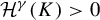 $ \mathcal {H}^{\gamma }(K)> 0 $
. By Proposition 2.2, let
 $ \mu $
be the unique measure of maximal entropy on
 $ X $
. Then,
 $$ \begin{align} \mu(I) \approx \exp(-k h(X)) \quad \text{for } I \in \mathcal{L}_{k}(X). \end{align} $$
For
 $ x \in X $
and
 $ k \in \mathbb {N} $
,
 $$ \begin{align*} R\mu(Q_{k}(x)) & = \sum_{I \in \Gamma_{k}(x)} \mu(I) && \!\kern-1pt\text{(by Lemma}~{2.6}) \\ & \approx \exp(-k h(X)) \cdot \#\Gamma_{k}(x) && \!\kern-1pt\text{(by}~({4.3}))\\ & \lesssim \exp\bigg ( \kern-1pt{-}\, k \bigg (h(X) \kern1.3pt{-}\kern0.9pt \sum_{i=1}^{s} (\theta_{i} - \theta_{i-1}) (h(X)-h(X_{i})) \kern-1pt\bigg ) \kern-1.7pt\bigg ) && \kern-1pt\!\text{(by Lemma}~{4.1}) \\ & = \exp \bigg( - k \bigg ( \sum_{i=1}^{s}(\theta_{i}-\theta_{i-1})h(X_{i})\bigg ) \bigg) && \!\kern-1pt\text{(by } \theta_{s} = 1,\, \theta_{0} = 0 ) \\ & = n_{s}^{-k\gamma} && \!\kern-1pt\text{(by}~({4.2})). \end{align*} $$
This shows
 $ \mathcal {H}^{\gamma }(K) \gtrsim 1 $
by Lemma 2.9.
Next, we prove
 $ \mathcal {H}^{s}(K) < \infty $
. Since
 $ \mathcal {Q}_{k}(X) $
covers
 $ K $
by the k-level approximate cubes with side lengths
 $ \approx n_{s}^{-k} $
, Lemma 3.2 implies that for some
 $ C> 0 $
,
 $$ \begin{align*} \mathcal{H}^{\gamma}_{Cn_{s}^{-k}}({K}) \lesssim n_{s}^{- k \gamma} \cdot \# \mathcal{Q}_{k}(X) \approx n_{s}^{- k \gamma} \exp \bigg ( k \sum_{i=1}^{s}(\theta_{i}-\theta_{i-1}) h(X_{i})\bigg) = 1, \end{align*} $$
where the last equality is by (4.2). Letting
 $ k \to \infty $
gives
 $ \mathcal {H}^{\gamma }(K) \lesssim 1 $
.
5 Proof of Theorem 1.1(ii) and (iii)
Theorem 1.1(ii) is contained in Proposition 5.2. Theorem 1.1(iii) follows by combining Lemma 5.3 with Theorem 1.1(i) and (ii).
5.1 Proof of Theorem 1.1(ii)
We first show that the Hausdorff measures of R-images of cylinders with the same length are comparable to each other.
Lemma 5.1. Let
 $ X $
be a subshift satisfying weak specification and
 $ K = R(X)$
. Let
 $ \varphi $
be a gauge function. Then, for
 $ k \in \mathbb {N} $
and
 $ I \in \mathcal {L}_{k}(X)$
,
 $$ \begin{align*} \mathcal{H}^{\varphi}(R([I]) \operatorname*{\mathrm{\cap}} K ) \approx \mathcal{H}^{\varphi}(\Lambda^{-k} K). \end{align*} $$
Proof. For
 $ J \in \mathcal {L}(X)$
, write
 $ \mathcal {D}_{J} = \{ j \in \mathcal {A} \colon Jj \in \mathcal {L}(X)\}$
. By the translation-invariance of
 $ \mathcal {H}^{\varphi }$
and (2.15),
 $$ \begin{align} \mathcal{H}^{\varphi}(R([J]\operatorname*{\mathrm{\cap}} X)) = \sum_{j\in\mathcal{D}_{J}} \mathcal{H}^{\varphi}(R([Jj]\operatorname*{\mathrm{\cap}} X)) = \sum_{j\in\mathcal{D}_{J}} \mathcal{H}^{\varphi}(\Lambda^{-\lvert J\rvert}R([j]\operatorname*{\mathrm{\cap}} X)). \end{align} $$
Then, since
 $ \mathcal {D}_{I} \subset \mathcal {L}_{1}(X)$
,
 $ X = \operatorname *{\mathrm {\bigcup }}_{j\in \mathcal {L}_{1}(X)} [j]\operatorname *{\mathrm {\cap }} X$
, and
 $ K = R(X)$
,
 $$ \begin{align} \mathcal{H}^{\varphi}(R([I]\operatorname*{\mathrm{\cap}} X)) \leq \sum_{j\in\mathcal{L}_{1}(X)} \mathcal{H}^{\varphi}(\Lambda^{-k}R([j]\operatorname*{\mathrm{\cap}} X)) = \mathcal{H}^{\varphi}(\Lambda^{-k}R(X)) = \mathcal{H}^{\varphi}(\Lambda^{-k}K). \end{align} $$
Next, we give a lower bound on
 $\mathcal {H}^{\varphi }(R([I]\operatorname *{\mathrm {\cap }} X))$
. Let
 $ p $
be as in Definition 2.1. For
 $ j \in \mathcal {L}_{1}(X) $
, there exists
 $ W \in \mathcal {L}(X)$
with
 $ \lvert W\rvert \leq p $
such that
 $ I W j \in \mathcal {L}(X)$
. Then,
 $$ \begin{align} \begin{aligned} \mathcal{H}^{\varphi}(R([I]\operatorname*{\mathrm{\cap}} X)) & \geq \mathcal{H}^{\varphi}(R( [IWj] \operatorname*{\mathrm{\cap}} X ) ) \\ & \geq \mathcal{H}^{\varphi}(\Lambda^{-k-\lvert W\rvert} R([j]\operatorname*{\mathrm{\cap}} X) ) & \text{(by}~({5.1})) \\ & \geq \mathcal{H}^{\varphi}(\Lambda^{-k-p} R([j]\operatorname*{\mathrm{\cap}} X) ), \end{aligned} \end{align} $$
where the last inequality is by
 $ \lvert W\rvert \leq p $
and
 $ \Lambda ^{-1}$
is contracting. Summing (5.3) over
 $ j \in \mathcal {L}_{1}(X)$
gives
 $$ \begin{align} \mathcal{H}^{\varphi}(R([I]\operatorname*{\mathrm{\cap}} X)) \geq \frac{1}{\#\mathcal{A}}\mathcal{H}^{\varphi}(\Lambda^{-k-p} R(X)). \end{align} $$
Notice that
 $ \Lambda ^{-k} T^{-p}(E) = \Lambda ^{-k-p}E + \Lambda ^{-k} \sum _{J\in \mathcal {A}^{p}} R_{p}(J)$
for
 $ E \subset \mathbb {T}^{d}$
. By the translation-invariance of
 $\mathcal {H}^{\varphi }$
,
 $$ \begin{align*} \mathcal{H}^{\varphi}(\Lambda^{-k-p} E) = \frac{1}{(\# \mathcal{A})^{p}} \mathcal{H}^{\varphi}(\Lambda^{-k}T^{-p}(E)). \end{align*} $$
Then, by (5.4), taking
 $ E = R(X) $
in the above equation implies that
 $$ \begin{align} \mathcal{H}^{\varphi}(R([I]\operatorname*{\mathrm{\cap}} X)) \geq \frac{1}{(\#\mathcal{A})^{p+1}}\mathcal{H}^{\varphi}(\Lambda^{-k}T^{-p}(R(X))) \geq \frac{1}{(\#\mathcal{A})^{p+1}}\mathcal{H}^{\varphi}(\Lambda^{-k}K), \end{align} $$
where the last inequality is by
 $ K = R(X)$
and
 $ K \subset T^{-p}(K) $
. Combining (5.2) and (5.5) finishes the proof.
Now, we are ready to prove Theorem 1.1(ii), which is contained in the following proposition.
Proposition 5.2. Let X be a subshift satisfying weak specification and
 $ K = R(X)$
. Let
 $ \mu $
be the measure of maximal entropy on
 $ X $
. If
 $ 0 < \mathcal {H}^{\varphi }(K) < \infty $
for some gauge function
 $ \varphi $
, then
 $$ \begin{align*} R\mu \approx \mathcal{H}^{\varphi}|_{K}, \end{align*} $$
where
 $ \mathcal {H}^{\varphi }|_{K} $
denotes the restriction of
 $ \mathcal {H}^{\varphi } $
to
 $ K $
. In particular,
 $ \dim _{\mathrm {H}} R\mu = \dim _{\mathrm {H}} K $
.
Proof. Fix any
 $ k \in \mathbb {N} $
. By Lemma 5.1,
 $$ \begin{align} \mathcal{H}^{\varphi}(R([I])\operatorname*{\mathrm{\cap}} K ) \approx \mathcal{H}^{\varphi}(R([J]) \operatorname*{\mathrm{\cap}} K) \quad\text{for } I, J \in \mathcal{L}_{k}(X). \end{align} $$
Since
 $ 0 < \mathcal {H}^{\varphi }(K) < \infty $
and
 $ \{ R([I])\}_{I\in \mathcal {L}_{k}(X)}$
covers
 $ K $
,
 $$ \begin{align} 1 \approx \mathcal{H}^{\varphi}|_{K}(K) = \sum_{I \in \mathcal{L}_{k}(X)} \mathcal{H}^{\varphi}|_{K}(R([I])). \end{align} $$
Combining (5.6) and (5.7) gives
 $$ \begin{align*} \mathcal{H}^{\varphi}|_{K}(R([I])) \approx \frac{1}{\# \mathcal{L}_{k}(X)} \quad \text{for } I \in \mathcal{L}_{k}(X). \end{align*} $$
Then, Proposition 2.2 implies that
 $$ \begin{align*} R\mu(R([I])) = \mu(I) \approx \frac{1}{\# \mathcal{L}_{k}(X)} \approx \mathcal{H}^{\varphi}|_{K}(R([I])) \quad \text{for } I \in \mathcal{L}_{k}(X). \end{align*} $$
Note that
 $ R\mu (R([I])) = 0 = \mathcal {H}^{\varphi }|_{K}(R([I])) $
for
 $ I \in \mathcal {A}^{k}\setminus \mathcal {L}_{k}(X) $
since
 $\mu $
is supported on X. Hence,
 $$ \begin{align*} R\mu(R([I])) \approx \mathcal{H}^{\varphi}|_{K}(R([I])) \quad \text{for all } I \in \mathcal{A}^{k}. \end{align*} $$
This finishes the proof because the collection of sets
 $ \{ R([I]) \colon I \in \operatorname *{\mathrm {\bigcup }}_{k=1}^{\infty } \mathcal {A}^{k} \}$
generates the Borel
 $ \sigma $
-algebra of
 $ \mathbb {T}^{d} $
.
5.2 Proof of Theorem 1.1(iii)
The proof of Theorem 1.1(iii) follows immediately by combining the following proposition with Theorem 1.1(i) and (ii).
Proposition 5.3. Let
 $ X $
be a subshift satisfying weak specification and
 $ K = R(X)$
. Let
 $\mu $
be the measure of maximal entropy on
 $ X$
. Suppose
 $ s \leq 2 $
. If
 $\dim _{\mathrm {H}} R\mu = \dim _{\mathrm {H}} K $
, then
 $ \dim _{\mathrm {H}} K = \dim _{\mathrm {B}} K $
.
Proof. By the definition of
 $ \mu $
and the assumption on
 $ \mu $
,
 $$ \begin{align*} h(\mu) = h(X) \quad\text{and}\quad \dim_{\mathrm{H}} R\mu = \dim_{\mathrm{H}} K. \end{align*} $$
When
 $ s = 1 $
. By Propositions 2.4 and 3.3,
 $$ \begin{align*} \dim_{\mathrm{H}} K = \dim_{\mathrm{H}} R\mu = \mathrm{d}_{\mathrm{LY}}(\mu) = \frac{h(\mu)}{\log n_{1}} = \frac{h(X)}{\log n_{1}} = \dim_{\mathrm{B}} K. \end{align*} $$
Alternatively, this follows from the result of Furstenberg [Reference Furstenberg20] since
 $ T $
is conformal.
When
 $ s = 2 $
. Recall
 $ \theta _{1} = \alpha _{2} \theta _{2} = \alpha _{2} $
from (2.7) and (2.13). By Lemma 2.5,
 $$ \begin{align} \dim_{\mathrm{H}} K = \frac{P}{\log n_{2} }, \end{align} $$
where
 $$ \begin{align} P = \lim_{k\to\infty} \frac{1}{k} \log \sum_{J \in \mathcal{L}_{k}(X_{2})} (\# \pi_{2}^{-1}(J))^{\theta_{1}}. \end{align} $$
Let
 $k \in \mathbb {N}$
and
 $ J \in \mathcal {L}_{k}(X_{2})$
. Since
 $ \tau _{2} = \pi _{2} $
, Proposition 2.4 implies that
 $$ \begin{align} \pi_{2}\mu(J) \approx \frac{(\# \pi_{2}^{-1}(J))^{\theta_{1}}}{\exp(kP)}. \end{align} $$
Since
 $ \mu (I) \approx \exp (-k h(X_{1})) $
for
 $ I \in \mathcal {L}_{k}(X_{1})$
by Proposition 2.2,
 $$ \begin{align} \pi_{2}\mu(J) = \sum_{I \in \pi_{2}^{-1} (J)} \mu(I) \approx \frac{\# \pi_{2}^{-1}(J)}{ \exp(kh(X_{1}))}. \end{align} $$
Combining (5.10) and (5.11) gives
 $$ \begin{align} (\# \pi_{2}^{-1}(J))^{\theta_{1}} \approx \exp\bigg (k \frac{\theta_{1}}{1 - \theta_{1} } (h(X_{1}) - P)\bigg ). \end{align} $$
By Proposition 2.2,
 $$ \begin{align} \#\mathcal{L}_{k}(X_{2}) \approx \exp(kh(X_{2})). \end{align} $$
Applying (5.12) and (5.13) to (5.9), we solve that
 $$ \begin{align*} P = \theta_{1} h(X_{1}) + (1-\theta_{1}) h(X_{2}). \end{align*} $$
This shows
 $ \dim _{\mathrm {H}} K = \dim _{\mathrm {B}} K $
by Proposition 3.3 and (5.8).
In the above proof, the assumption of
 $ s \leq 2 $
allows the potential
 $ \phi ^{(2)} $
as in (2.8) to be estimated by combining the Gibbs property of
 $ \mu $
and
 $\tau _{2} \mu $
. However, this argument does not extend to
 $ s \geq 3 $
due to the lack of the information about the regularity of
 $ \tau _{i} \mu $
for
 $ 2 \leq i \leq s - 1 $
. In fact, the examples in §7 show that Lemma 5.3 does not hold when
 $ s \geq 3 $
.
6 Bedford–McMullen sponges
This section is devoted to the results about Bedford–McMullen sponges. The proof of Theorem 1.2 is given in §6.2.
6.1 Dimensional results
In this subsection, we include some results of Kenyon and Peres about the dimensions of Bedford–McMullen sponges. Let
 $\mathcal {D}$
be a non-empty subset of
 $ \mathcal {A}$
. Define
 $ \mathcal {D}_{i} = \tau _{i} (\mathcal {D}) $
for
 $ 1\leq i \leq s $
. Define
 $ Z^{(1)} \equiv 1 $
on
 $\mathcal {D}_{1} $
. For
 $ 2 \leq i \leq s $
, recursively define
 $$ \begin{align} Z^{(i)}(x) = \sum_{y\in \mathcal{D}_{i-1} \colon \pi_{i}(y) = x } Z^{(i-1)}(y)^{\alpha_{i-1}} \quad\text{for } x \in \mathcal{D}_{i}. \end{align} $$
Define
 $$ \begin{align} Z = \sum_{x \in \mathcal{D}_{s}} Z^{(s)}(x)^{\alpha_{s}}. \end{align} $$
Proposition 6.1. [Reference Kenyon and Peres26, Theorem 1.2]
Let
 $ K = R(\mathcal {D}^{\mathbb {N}}) $
for some
 $ \emptyset \neq \mathcal {D} \subset \mathcal {A} $
. Then,
 $$ \begin{align*} \dim_{\mathrm{H}} K = \frac{\log Z}{\log n_{s}}, \end{align*} $$
where
 $ Z $
is as in (6.2). There is a unique measure of full dimension
 $\eta _{p} $
which is the Bernoulli measure with marginal
 $ p = p(x)_{x\in \mathcal {D}} $
, where
 $$ \begin{align} p(x) = \frac{1}{Z} \prod_{i = 1}^{s} Z^{(i)}(\tau_{i}(x))^{\alpha_{i}-1} \quad\text{for } x \in \mathcal{D}. \end{align} $$
There is a simple criterion for Bedford–McMullen sponges to have equal Hausdorff and box dimensions. For
 $ 1 \leq i \leq s $
, define
 $$ \begin{align} f_{i}(x) = \#\pi_{i}^{-1}(\tau_{i}(x)) \quad\text{for } x \in \mathcal{D}. \end{align} $$
Proposition 6.2. [Reference Kenyon and Peres26, Proposition 1.3]
Let
 $ K = R(\mathcal {D}^{\mathbb {N}}) $
for some
 $\emptyset \neq \mathcal {D} \subset \mathcal {A} $
. Then,
 $\dim _{\mathrm {H}} K = \dim _{\mathrm {B}} K$
if and only if
 $$ \begin{align} f_{i}(x) = f_{i}(y) \quad \text{ for all } 1 \leq i \leq s \text{ and } x, y\in \mathcal{D}. \end{align} $$
As a direct corollary of Proposition 6.1, the following condition characterizes when the measures of maximal entropy and full dimension coincide.
Corollary 6.3. Let
 $ K = R(\mathcal {D}^{\mathbb {N}}) $
for some
 $ \emptyset \neq \mathcal {D} \subset \mathcal {A} $
. Then, the measures of maximal entropy and full dimension coincide if and only if
 $$ \begin{align} \prod_{i = 1}^{s} Z^{(i)}(\tau_{i}(x))^{\alpha_{i}-1} = \prod_{i = 1}^{s} Z^{(i)}(\tau_{i}(y))^{\alpha_{i}-1} \quad\text{for } x, y \in \mathcal{D}. \end{align} $$
When
 $ s \leq 3 $
, (6.6) is equivalent to
 $$ \begin{align} \prod_{i=1}^{s} f_{i}(x)^{\theta_{i-1}-1} = \prod_{i=1}^{s} f_{i}(y)^{\theta_{i-1}-1} \quad\text{for } x, y \in \mathcal{D}. \end{align} $$
Proof. Since the measure of maximal entropy on
 $ \mathcal {D}^{\mathbb {N}}$
is the Bernoulli measure with marginal
 $(1/\#\mathcal {D}, \ldots , 1/\#\mathcal {D})$
, the first equivalence follows directly from Proposition 6.1. Next, we show the second equivalence. Since
 $ f_{1}(x) = Z^{(1)}(x) = 1 $
and
 $ f_{2}(x) = Z^{(2)}(\tau _{2}(x)) $
for
 $ x\in \mathcal {D}$
, (6.6) and (6.7) are equivalent when
 $ s \leq 2 $
. Suppose
 $ s = 3 $
. Let
 $ x \in \mathcal {D}$
. For
 $ z \in \pi _{3}^{-1}(\tau _{3}(x)) $
, there exists
 $ y \in \mathcal {D} $
such that
 $ \tau _{2}(y) = z $
, and so
 $ \tau _{3}(y) = \pi _{3}(\tau _{2}(y)) = \pi _{3}(z) = \tau _{3}(x)$
. Then, either (6.6) or (6.7) implies
 $ f_{2}(x) = f_{2}(y) $
, and thus
 $ Z^{(2)}(z) = Z^{(2)}(\tau _{2}(y)) = f_{2}(y) = f_{2}(x)$
. Hence, by (6.1),
 $$ \begin{align*} Z^{(3)}(\tau_{3}(x)) = \sum_{z \in \pi_{3}^{-1}(\tau_{3}(x))} Z^{(2)}(z)^{\alpha_{2}} = f_{3}(x) f_{2}(x)^{\alpha_{2}}. \end{align*} $$
Thus,
 $$ \begin{align*} \prod_{i = 1}^{3} Z^{(i)}(\tau_{i}(x))^{\alpha_{i}-1} = f_{2}(x)^{\alpha_{2}-1} (f_{3}(x) f_{2}(x)^{\alpha_{2}} )^{\alpha_{3}-1} = f_{2}(x)^{\theta_{1}-1}f_{3}(x)^{\theta_{2}-1}, \end{align*} $$
which finishes the proof.
It is easy to see that (6.5) is equivalent to (6.7) if
 $ s \leq 2 $
, but stronger than (6.7) if
 $ s = 3 $
. This motivates us to give the examples in §7.
6.2 Proof of Theorem 1.2
Let
 $ X $
be a subshift and
 $\mu $
be a measure on X. For a gauge function
 $\varphi $
, define
 $$ \begin{align*} \Theta_{k}^{\varphi}(\mu, x) = \frac{R\mu(Q_{k}(x))}{\varphi(n_{s}^{-k})} \quad\text{for } x \in X \text{ and } k\in \mathbb{N}. \end{align*} $$
Write
 $ \Theta _{k}^{\varphi } $
as
 $ \Theta _{k}^{\gamma } $
when
 $\varphi (r) = r^{\gamma }$
for some
 $ \gamma \geq 0 $
. Let
 $ E[X] $
and
 $ \operatorname {\mathrm {Var}}(X)$
respectively denote the expectation and variance of a random variable
 $ X $
.
Proof of Theorem 1.2
By Theorem 1.1(i), it remains to show that if
 $ 0 < \mathcal {H}^{\varphi }(K) < \infty $
for some gauge function
 $ \varphi $
, then
 $ \dim _{\mathrm {H}} K = \dim _{\mathrm {B}} K $
.
Suppose
 $ 0 < \mathcal {H}^{\varphi }(K) < \infty $
. Write
 $ K = R(\mathcal {D}^{\mathbb {N}})$
for some
 $ \mathcal {D} \subset \mathcal {A} $
. Let
 $ \mu $
be the measure of maximal entropy on
 $ \mathcal {D}^{\mathbb {N}} $
, that is,
 $ \mu $
is the Bernoulli measure with marginal
 $ ( 1/ \# \mathcal {D}, \ldots , 1/\# \mathcal {D})$
. Let
 $ x = (x_{j})_{j=1}^{\infty } \in \mathcal {D}^{\mathbb {N}}$
be a random sequence with law
 $\mu $
. For
 $ k \in \mathbb {N} $
and
 $ 1 \leq j \leq k $
, define the random variables
 $$ \begin{align} X_{j}^{(k)} = \log \# \tau_{i}^{-1}(\tau_{i}(x_{j})) \quad\text{for } 1 \leq i \leq s \text{ and } \lfloor \theta_{i-1} k \rfloor + 1 \leq j \leq \lfloor \theta_{i} k \rfloor. \end{align} $$
Note that
 $ x_{1}, \ldots , x_{k}$
are independent and identically distributed random variables with common law
 $ \sum _{y\in \mathcal {D}} 1/(\#\mathcal {D}) \delta _{y} $
. Then,
 $ X_{1}^{(k)}, \ldots , X_{k}^{(k)} $
are independent and uniformly bounded. Write
 $ E_{k} = \sum _{j=1}^{k} E[ X_{j}^{(k)}]$
and
 $ V_{k}^{2} = \sum _{j=1}^{k} \operatorname {\mathrm {Var}}( X_{j}^{(k)}) $
. For
 $ k \in \mathbb {N} $
, define
 $$ \begin{align} L(k) = \log ( (\#\mathcal{D})^{k} \varphi(n_{s}^{-k}) ). \end{align} $$
For
 $ x = (x_{j})_{j=1}^{\infty } \in \mathcal {D}^{\mathbb {N}} $
and
 $ k \in \mathbb {N} $
, (2.17) implies
 $$ \begin{align} \begin{aligned} \# \Gamma_{k}(x) & = \# \big\{ I \in \mathcal{L}_{k}(\mathcal{D}^{\mathbb{N}}) \colon \tau_{i}(I|_{\lfloor \theta_{i-1} k \rfloor }^{\lfloor \theta_{i} k \rfloor } ) = \tau_{i}(x|_{\lfloor \theta_{i-1} k \rfloor }^{\lfloor \theta_{i} k \rfloor }) \text{ for } 1 \leq i \leq s \big\} \\ & = \prod_{i=1}^{s}\prod_{j=\lfloor \theta_{i-1} k \rfloor +1}^{\lfloor \theta_{i} k \rfloor } \# \tau_{i}^{-1}(\tau_{i}(x_{j})). \end{aligned} \end{align} $$
Since
 $ \mu (I) = 1/(\#\mathcal {D})^{k}$
for
 $ I \in \mathcal {D}^{k}$
, Lemma 2.6 shows
 $$ \begin{align} \begin{aligned} R\mu(Q_{k}(x)) & = \sum_{I \in \Gamma_{k}(x)} \mu(I) = \frac{ \#\Gamma_{k}(x)}{(\# \mathcal{D})^{k}}. \end{aligned} \end{align} $$
Combining (6.8), (6.9), (6.10), and (6.11) gives
 $$ \begin{align} \Theta_{k}^{\varphi}(\mu, x) = \exp \bigg( \kern-2pt\sum_{j=1}^{k} X_{j}^{(k)} - L(k) \bigg) \quad\text{for } x \in \mathcal{D}^{\mathbb{N}}. \end{align} $$
By Proposition 5.2 and the upper density theorem for the Hausdorff measures (see Proposition B.1 or [Reference Davies and Samuels10]), there exists
 $ C> 0 $
such that
 $$ \begin{align*} \mu \bigg \{ x \colon \frac{1}{C} \leq \limsup_{k\to\infty} \Theta_{k}^{\varphi}(\mu, x) \leq C \bigg\} = 1. \end{align*} $$
From this and (6.12), there exists
 $ M> 0 $
such that
 $$ \begin{align} \mathbb{P} \bigg \{ \limsup_{k\to\infty} \bigg\lvert\!\sum_{j=1}^{k} X_{j}^{(k)} - L(k) \bigg\rvert < M \bigg \} = 1, \end{align} $$
where
 $ \mathbb {P} $
denotes the underlying probability (that is, a probabilistic notation for
 $ \mu $
).
Suppose on the contrary that
 $ \dim _{\mathrm {H}} K < \dim _{\mathrm {B}} K $
. It follows from Proposition 6.2 that
 $ \# \tau _{i_{0}}^{-1}(\tau _{i_{0}}(x)) \neq \# \tau _{i_{0}}^{-1}(\tau _{i_{0}}(y))$
for some
 $ 1 \leq i_{0} \leq s $
and
 $ x, y \in \mathcal {D}$
. Let
 $ Y $
be the random variable with law
 $ \sum _{x\in \mathcal {D}} (1/\#\mathcal {D}) \delta _{\# \tau _{i_{0}}^{-1}(\tau _{i_{0}}(x))}$
, then
 $ \operatorname {\mathrm {Var}}(Y)> 0 $
. By (6.8),
 $Y $
has the same law as
 $ X_{j}^{(k)}$
for
 $ \lfloor \theta _{i-1} k \rfloor +1 \leq j \leq \lfloor \theta _{i} k \rfloor $
. Then, by the independence of
 $ X_{j}^{(k)}$
,
 $$ \begin{align*} V_{k}^{2} \geq \sum_{j=\lfloor \theta_{i-1} k \rfloor +1}^{\lfloor \theta_{i} k \rfloor } \operatorname{\mathrm{Var}}(X_{j}^{(k)}) \gtrsim \operatorname{\mathrm{Var}}(Y) (\theta_{i} - \theta_{i-1}) k \, \to \infty, \end{align*} $$
as
 $ k \to \infty $
. By Lyapunov’s central limit theorem (see e.g. [Reference Chung7, Theorem 7.1.2]), the normalized random sum
 $ Y_{k} = (\sum _{j=1}^{k} X_{j}^{(k)} - E_{k})/ V_{k}$
converges to the standard normal random variable
 $ N(0,1) $
in distribution. Since the distribution of
 $ N(0,1)$
is absolutely continuous and
 $ \lim _{k\to \infty } M/V_{k} = 0 $
,
 $$ \begin{align} \begin{aligned} \mathbb{P} \bigg\{ \bigg\lvert\kern-2pt\sum_{j=1}^{k} X_{j}^{(k)} - L(k) \bigg\rvert < M \bigg\} = \mathbb{P} \bigg\{ \bigg\lvert Y_{k} - \frac{L(k)-E_{k}}{V_{k}} \bigg\rvert < \frac{M}{V_{k}} \bigg\} \to 0, \end{aligned} \end{align} $$
as
 $ k \to \infty $
. This implies
 $$ \begin{align*} \mathbb{P} \bigg \{\kern-3pt \limsup_{k\to\infty} \bigg\lvert\kern-3pt\sum_{j=1}^{k} X_{j}^{(k)} - L(k) \bigg\rvert < M \bigg \} \leq \limsup_{k\to\infty} \mathbb{P} \bigg \{ \bigg\lvert\kern-3pt\sum_{j=1}^{k} X_{j}^{(k)} - L(k) \bigg\rvert < M \bigg \} = 0, \end{align*} $$
which contradicts (6.13).
Remark 6.4. The proof of Theorem 1.2 works for some other subshift X satisfying weak specification if we can write
 $\log R\mu (Q_{k}(x))$
as a sequence of random variables such that a certain limit theorem can be applied to conclude an analog of (6.14). Next, we give an example to illustrate it. Let
 $m_{1}, m_{2}, m_{3}$
be integers such that
 $ m_{1}> m_{2} > m_{3} \geq 2, m_{1}, m_{2} \geq 3$
. Let
 $ \mathcal {A}, \theta _{i}, \pi _{i}, \tau _{i}, 1 \leq i \leq s = 3 $
be defined as in §2.1. Let
 $$ \begin{align*} \mathcal{D} = \left \{ \begin{pmatrix}0 \\ 0 \\ 0\end{pmatrix}, \begin{pmatrix}0 \\ 1 \\ 0\end{pmatrix}, \begin{pmatrix}1 \\ 1 \\ 0\end{pmatrix}, \begin{pmatrix}0 \\ 2 \\ 1\end{pmatrix}, \begin{pmatrix}1 \\ 2 \\ 1\end{pmatrix}, \begin{pmatrix}2 \\ 2 \\ 1\end{pmatrix} \right \}. \end{align*} $$
Enumerate
 $\mathcal {D}$
as
 $ \{ z_{1}, \ldots , z_{6}\}$
according to the above order. Let
 $ A = (A_{i,j}) $
be a
 $ 6 \times 6 $
matrix such that
 $ A_{i,i} = 0 $
and
 $ A_{i,j} = 1$
if
 $ i \neq j$
for
 $ 1 \leq i, j \leq 6$
. Consider the following subshift of finite type:
 $$ \begin{align*} \Sigma_{A} &= \{ (x_{k})_{k=1}^{\infty} \in \mathcal{D}^{\mathbb{N}} \colon \text{ for all }\, k \in \mathbb{N}, \\ &\qquad\text{there exists }\, 1\leq i, j\leq 6, \, x_{k} = z_{i}, x_{k+1} = z_{j}, \, A_{i,j} = 1 \}. \end{align*} $$
Let
 $ K = R(\Sigma _{A})$
. By [Reference Parry35] (see also [Reference Walters41]), the unique measure of maximal entropy
 $\mu $
on
 $ \Sigma _{A} $
is the Markov measure generated by the probability vector
 $ (1/6, \ldots , 1/6)$
and the random matrix
 $ A / 5 $
. By computation,
 $ \tau _{2}\mu $
is the Markov measure on
 $ \tau _{2}(\Sigma _{A})$
generated by
 $ (1/6, 1/3, 1/2)$
and
 $ \bigg (\!\begin {smallmatrix} 0 & 2/5 & 3/5 \\ 1/5& 1/5 & 3/5 \\ 1/5& 2/5 & 2/5 \end {smallmatrix}\!\bigg ) $
. Since the computation shows that
 $ \tau _{2}\mu $
is not the measure of maximal entropy on
 $ \tau _{2}(\Sigma _{A})$
, it follows from Theorem 3.1(b) that
 $ \dim _{\mathrm {H}} K < \dim _{\mathrm {B}} K $
. By the definition of
 $ \mathcal {D} $
, a similar estimate as in the proof of Theorem 1.2 gives
 $$ \begin{align*} \log R\mu(Q_{k}(x)) \approx \theta_{1} k + 3 (1-\theta_{2}) k + \sum_{j = \lfloor \theta_{1} k \rfloor + 1}^{\lfloor \theta_{2} k \rfloor} Y((\tau_{2}x)_{j}), \end{align*} $$
where
 $ Y \colon \tau _{2}\mathcal {D} \to \{1,2,3\} $
is a function defined as
 $ Y((0, 0)^{t}) = 1, Y((1, 0)^{t}) = 2$
and
 $ Y((2, 1)^{t}) = 3 $
. Since the law of
 $\tau _{2}x$
is the Markov measure
 $ \tau _{2}\mu $
if
 $ x $
is a random sequence with law
 $ \mu $
, we can apply the central limit theorem for Markov chains (see e.g. [Reference Durrett11, Example 8.3.4]) and adapt the proof of Theorem 1.2 to conclude that
 $ \mathcal {H}^{\varphi }(K) = 0 $
or
 $\infty $
for every gauge function
 $ \varphi $
.
6.3 Infinite Hausdorff measure
In this subsection, we provide a sufficient condition (see Proposition 6.6) for Bedford–McMullen sponges to have infinite Hausdorff measures at their respective Hausdorff dimensions. This is based on the method of Peres [Reference Peres37] and a relation (see Lemma 6.8) satisfied by the measure of full dimension. In [Reference Peres37, §5], Peres mentioned that [Reference Peres37, Theorem 1 and Proposition 2] can extend to Bedford–McMullen sponges. However, he did not give a detailed justification. In fact, the proof of [Reference Peres37, Proposition 2] does not work for Bedford–McMullen sponges, as indicated by the examples in §7. For the extension of [Reference Peres37, Theorem 1], it is not clear how to construct a measure with zero density like that in the proof of [Reference Peres37, Theorem 1] since the measure of full dimension becomes more complicated when
 $ s \geq 3 $
(see Proposition 6.1).
Throughout this subsection, we fix a non-empty subset
 $ \mathcal {D} $
of
 $ \mathcal {A} $
and let
 $ K = R(\mathcal {D}^{\mathbb {N}})$
. Let
 $p = (p(x))_{x\in \mathcal {D}} $
be the probability vector given in (6.3). Write
 $ \gamma = \dim _{\mathrm {H}} K $
. For a finite set
 $ \mathcal {B} $
and probability vectors
 $ q = (q(x))_{x \in \mathcal {B}}$
and
 $ q' = (q'(x))_{x\in \mathcal {B}}$
, following [Reference Peres37], we define
 $$ \begin{align} \Delta(q\| q') = \sum_{x \in \mathcal{B}} (q(x)- q'(x)) \log q(x), \end{align} $$
where we require
 $ q'(x) = 0 $
if
 $ q(x) = 0 $
.
The following proposition is essentially contained in [Reference Peres37]. For completeness, we include a proof of Proposition 6.5 in Appendix A.
Proposition 6.5. (Peres [Reference Peres37])
If there exist a probability vector
 $ q $
on
 $\mathcal {D} $
and
 $ c> 0 $
such that
 $$ \begin{align} \sum_{i=1}^{s} \Delta(\tau_{i}p\| \tau_{i} q) \int_{\theta_{i-1}k}^{\theta_{i}k} \frac{1}{\log t} \,d t \geq c \frac{k}{(\log k)^{2}} \quad\text{for large } k \in \mathbb{N}, \end{align} $$
then
 $ \mathcal {H}^{\varphi }(K) = \infty $
, where
 $$ \begin{align} \varphi(r) = r^{\gamma} \exp\bigg(\kern-2pt-\widetilde{c} \frac{\lvert\log r\rvert}{(\log \lvert\log r\rvert)^{2}} \bigg), \quad r> 0, \end{align} $$
for some
 $ \widetilde {c}> 0 $
depending on
 $ c $
explicitly. In particular,
 $ \mathcal {H}^{\gamma }(K) = \infty $
.
In the remaining part of this subsection, we prove the following proposition which is a sufficient condition such that the Hausdorff measures of Bedford–McMullen sponges are infinite at their Hausdorff dimensions. We do not expect condition (6.18) to be necessary, but it is sufficient for determining the Hausdorff measure of the examples in §7 at their respective Hausdorff dimensions. For a probability vector
 $ q = (q(x))_{x\in \mathcal {B}}$
on a finite set
 $\mathcal {B} $
, we say
 $q $
is uniform if
 $q = (1/\#\mathcal {B}, \ldots , 1/\#\mathcal {B})$
.
Proposition 6.6. If
 $$ \begin{align} 1 \leq \# \{ 1 \leq i \leq s \colon \tau_{i} p \text{ is not uniform}\} \leq 2, \end{align} $$
then
 $ \mathcal {H}^{\dim _{\mathrm {H}} K}(K) = \infty $
.
Proposition 6.6 extends some results in [Reference Peres37] since for Bedford–McMullen carpets, the upper bound in (6.18) trivially holds when
 $ d = 2 $
, and the lower bound in (6.18) follows from
 $ \dim _{\mathrm {H}} K < \dim _{\mathrm {B}} K $
and Theorem 3.1(b). Next, we give two lemmas for the proof of Proposition 6.6.
Lemma 6.7. If
 $ q $
is uniform, then
 $ \Delta (q \| q') = 0 $
. If
 $ q' $
is uniform but
 $ q $
is not uniform, then
 $\Delta (q\| q')> 0 $
.
Proof. The first statement is by a direct computation. The second statement follows from
 $$ \begin{align*} \Delta(q\| q') = \frac{1}{2\#\mathcal{B}} \sum_{x\in\mathcal{B}} \sum_{y\in\mathcal{B}} (q(x)-q'(y))(\log q(x)- \log q'(y))> 0, \end{align*} $$
when
 $ q' $
is uniform.
The following lemma is the key ingredient for the verification of condition (6.16) when
 $ s \geq 3 $
.
Lemma 6.8. For every probability vector
 $ q $
on
 $ \mathcal {D} $
,
 $$ \begin{align} \sum_{i=1}^{s} (\theta_{i}- \theta_{i-1})\Delta( \tau_{i}p\| \tau_{i} q) = 0. \end{align} $$
Proof. For
 $ 1\leq i \leq s $
, write
 $ p_{i} = \tau _{i}p $
,
 $ q_{i} = \tau _{i} q $
, and
 $\Delta _{i} = \Delta (p_{i}\| q_{i})$
. By (6.15),
 $$ \begin{align*} \begin{aligned} \Delta_{i} & = \sum_{x \in \mathcal{D}_{i}} (p_{i}(x)-q_{i}(x)) \log p_{i}(x) &&\\ & = \sum_{x\in\mathcal{D}_{i}} \log p_{i}(x) \sum_{y\in\tau_{i}^{-1}(x)} (p_{1}(y) - q_{1}(y)) && \text{(by }p_{i}=\tau_{i}p_{1}, q_{i}=\tau_{i}q_{1})\\ & = \sum_{x\in\mathcal{D}_{i}} \sum_{y\in\tau_{i}^{-1}(x)} (p_{1}(y) - q_{1}(y))\log p_{i}(\tau_{i}(y)) && \text{(by } \tau_{i}(y) = x \text{ for } y \in \tau_{i}^{-1}(x))\\ & = \sum_{y\in\mathcal{D}_{1}} (p_{1}(y) - q_{1}(y))\log p_{i}(\tau_{i}(y)).&& \end{aligned} \end{align*} $$
Then,
 $$ \begin{align*} \begin{aligned} \sum_{i=1}^{s} (\theta_{i}- \theta_{i-1})\Delta_{i} & = \sum_{x\in\mathcal{D}_{1}} (p_{1}(x) - q_{1}(x)) \sum_{i=1}^{s} (\theta_{i}-\theta_{i-1}) \log p_{i}(\tau_{i}(x)). \end{aligned} \end{align*} $$
Since
 $ \sum _{x\in \mathcal {D}_{1}}p_{1}(x) = \sum _{x\in \mathcal {D}_{1}} q_{1}(x) = 1$
, it suffices to show
 $$ \begin{align} \sum_{i=1}^{s} (\theta_{i}-\theta_{i-1}) \log p_{i}(\tau_{i}(x)) = - \log Z \quad\text{for } x \in \mathcal{D}_{1}. \end{align} $$
By (6.3), for
 $ x \in \mathcal {D}_{1}$
and
 $ 2 \leq i \leq s$
,
 $$ \begin{align*} p_{1}(x) = p_{i}(\tau_{i}(x)) \frac{1}{Z^{(i)}(\tau_{i}(x))} \prod_{j=1}^{i-1} Z^{(j)}(\tau_{j}(x))^{\alpha_{j}-1}. \end{align*} $$
Thus,
 $$ \begin{align*} \begin{aligned} \sum_{i=1}^{s} & (\theta_{i}-\theta_{i-1}) \log p_{i}(\tau_{i}(x)) \\ & = \log p_{1}(x) - \sum_{i=2}^{s} (\theta_{i-1}-\theta_{i}) Z^{(i)}(\tau_{i}(x)) - \sum_{i=2}^{s}\sum_{j=1}^{i-1} (\theta_{i}-\theta_{i-1}) (\alpha_{j}-1)\log Z^{(j)}(\tau_{j}(x)) \\ & = \log p_{1}(x) - \sum_{i=2}^{s} (\theta_{i-1}-\theta_{i}) Z^{(i)}(\tau_{i}(x)) - \!\sum_{j=1}^{s-1}\sum_{i=j+1}^{s} (\theta_{i}-\theta_{i-1}) (\alpha_{j}-1)\log Z^{(j)}(\tau_{j}(x)) \\ & = \log p_{1}(x) - \sum_{i=2}^{s} (\theta_{i-1}-\theta_{i}) Z^{(i)}(\tau_{i}(x)) - \sum_{j=1}^{s-1}(1-\theta_{j}) (\alpha_{j}-1)\log Z^{(j)}(\tau_{j}(x)) \\ & = \log p_{1}(x) - \sum_{i=1}^{s} (\alpha_{i}-1) Z^{(i)}(\tau_{i}(x)) \\ & = - \log Z, \end{aligned} \end{align*} $$
where the second equality is by changing the index of
 $i, j$
; the second last equality is by
 $ Z^{(1)} \equiv 1 $
and
 $ \theta _{i}\alpha _{i} = \theta _{i-1}$
for
 $ 1 \leq i \leq s$
; the last equality is by (6.3).
Now, we are ready to prove Proposition 6.6.
Proof of Proposition 6.6
For a probability vector
 $ q $
on
 $ \mathcal {D} $
and
 $ 1 \leq i \leq s $
, write
 $ p_{i} = \tau _{i}p $
,
 $ q_{i} = \tau _{i} q $
, and
 $\Delta _{i} = \Delta (p_{i}\| q_{i})$
. Define
 $ I = \{ 1 \leq i \leq s \colon p_{i} \text { is not uniform} \}$
. It follows from Lemma 6.7 that
 $ \Delta _{i} = 0 $
for
 $ i \notin I $
. By Lemma 6.8,
 $$ \begin{align} \sum_{i \in I} (\theta_{i}-\theta_{i-1}) \Delta_{i} = \sum_{i=1}^{s} (\theta_{i}-\theta_{i-1}) \Delta_{i} = 0. \end{align} $$
We first show
 $ \# I \neq 1 $
. Suppose otherwise that
 $ I = \{i_{1}\}$
. Take a probability vector
 $ q $
on
 $\mathcal {D}$
such that
 $ \tau _{i_{1}}q $
is uniform. Then,
 $ \Delta _{i_{1}}> 0 $
by Lemma 6.7, which contradicts (6.21). Then,
 $ \# I = 2 $
by assumption (6.18).
Write
 $ I = \{ i_{1}, i_{2}\}$
for some
 $ 1 \leq i_{1} < i_{2} \leq s $
. Take a probability vector
 $ q $
on
 $\mathcal {D}$
such that
 $ \tau _{i_{1}}q $
is uniform. Then,
 $ \Delta _{i_{1}}> 0 $
by Lemma 6.7. By (6.21),
 $$ \begin{align*} \Delta_{i_{2}} = - \frac{\theta_{i_{1}}-\theta_{i_{1}-1}}{\theta_{i_{2}}-\theta_{i_{2}-1}}\Delta_{i_{1}} < 0. \end{align*} $$
Since
 $ \Delta _{i} = 0 $
for
 $i \neq I$
,
 $$ \begin{align} \begin{aligned} \sum_{i=1}^{s} & \Delta_{i} \int_{\theta_{i-1}k}^{\theta_{i}k} \frac{1}{\log t} \,d t \\ & = \Delta_{i_{1}}(\theta_{i_{1}}-\theta_{i_{1}-1})\bigg( \frac{1}{\theta_{i_{1}}-\theta_{i_{1}-1}} \int_{\theta_{i_{1}-1}k}^{\theta_{i_{1}}k}\frac{1}{\log t} \, dt - \frac{1}{\theta_{i_{2}}-\theta_{i_{2}-1}} \int_{\theta_{i_{2}-1}k}^{\theta_{i_{2}}k}\frac{1}{\log t} \, dt \bigg). \end{aligned} \end{align} $$
By a change of variable, for
 $ 0 < a < b \leq c < d$
, there exists
 $ \delta> 0 $
such that
 $$ \begin{align} \frac{1}{b-a} \int_{ak}^{bk} \frac{1}{\log t} \, dt - \frac{1}{d-c} \int_{ck}^{dk} \frac{1}{\log t} \, dt \geq \delta \frac{k}{(\log k)^{2}} \quad\text{for } k \in \mathbb{N} \operatorname*{\mathrm{\cap}} \bigg [\frac{2}{a},\infty\bigg). \end{align} $$
Combining (6.22) and (6.23) verifies condition (6.16). Finally, the proof is completed by Proposition 6.5.
Remark 6.9. From the proof of Proposition 6.6, we see that
 $$ \begin{align} \# \{ 1 \leq i \leq s \colon \tau_{i}p \text{ is not uniform}\} \neq 1. \end{align} $$
Based on (6.24), there is an alternative way to prove that for a Bedford–McMullen carpet K,
 $ 0 < \mathcal {H}^{\varphi }(K) < \infty $
implies
 $ \dim _{\mathrm {H}} K = \dim _{\mathrm {B}} K $
. Suppose otherwise that
 $ \dim _{\mathrm {H}} K < \dim _{\mathrm {B}} K $
. Combining Proposition 5.2 and Theorem 3.1(b) gives
 $ \# \{ 1 \leq i \leq s \,{\colon} \tau _{i}p \text { is not uniform}\} = 1 $
, which contradicts (6.24).
7 Examples
In this section, we present several Bedford–McMullen sponges
 $K=R(\mathcal {D}^{\mathbb {N}})$
,
 $ \emptyset \neq \mathcal {D} \subset \mathcal {A} $
such that
 $ \dim _{\mathrm {H}} R\mu = \dim _{\mathrm {H}} K < \dim _{\mathrm {B}} K $
, where
 $ \mu $
is the measure of maximal entropy on
 $\mathcal {D}^{\mathbb {N}}$
. By Theorem 1.2, no gauge function exists for such sponges. For a finite set
 $ \mathcal {B}$
and a probability vector
 $ p = (p(x))_{x\in \mathcal {B}} $
, let
 $ \eta _{p} $
denote the Bernoulli measure on
 $ \mathcal {B}^{\mathbb {N}}$
with marginal p.
Example 7.1. Let
 $$ \begin{align*} \Lambda = \operatorname{\mathrm{diag}}(64, 16, 8) \end{align*} $$
and
 $$ \begin{align*} \mathcal{D} = \left \{ \begin{pmatrix}0 \\ 0 \\ 0\end{pmatrix}, \begin{pmatrix}0 \\ 1 \\ 0\end{pmatrix}, \begin{pmatrix}0 \\ 2 \\ 0\end{pmatrix}, \begin{pmatrix}0 \\ 3 \\ 0\end{pmatrix}, \begin{pmatrix}0 \\ 0 \\ 1\end{pmatrix}, \begin{pmatrix}1 \\ 0 \\ 1\end{pmatrix} \right \}. \end{align*} $$
Define
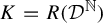 $ K = R( \mathcal {D}^{\mathbb {N}} ) $
. By Propositions 3.3 and 6.1,
 $$ \begin{align*} \dim_{\mathrm{B}} K = \frac{\log 360}{12 \log 2} \quad\text{and}\quad \dim_{\mathrm{H}} K = \frac{\log 18}{6 \log 2}. \end{align*} $$
The measure of maximal entropy is
 $ \eta _{p} $
with
 $ p = p_{1} = (1/6, 1/6, 1/6, 1/6, 1/6, 1/6 ) $
. Note that
 $ \tau _{2}\eta _{p_{1}} = \eta _{p_{2}} $
and
 $ \tau _{3}\eta _{p_{1}} = \eta _{p_{3}}$
, where
 $ p_{2} = (1/6, 1/6, 1/6, 1/6, 1/3)$
and
 $ p_{3} = (2/3, 1/3) $
. By Proposition 2.3,
 $$ \begin{align*} \begin{aligned} \dim_{\mathrm{H}} R \eta_{p} = \mathrm{d}_{\mathrm{LY}}(\eta_{p}) = \frac{\log 18}{6 \log 2}. \end{aligned} \end{align*} $$
Hence,
 $$ \begin{align*} \dim_{\mathrm{H}} R\eta_{p} = \dim_{\mathrm{H}} K < \dim_{\mathrm{B}} K. \end{align*} $$
Since
 $\#\{ 1 \leq i \leq 3 \colon p_{i} \text { is not uniform}\} = 2$
, it follows from Proposition 6.6 that
 $$ \begin{align*} \mathcal{H}^{\dim_{\mathrm{H}} K}(K) = \infty. \end{align*} $$
Next, we give similar examples when
 $ d \geq 4 $
.
Example 7.2. For
 $ d \geq 4 $
, let
 $$ \begin{align*} \Lambda = \operatorname{\mathrm{diag}} ( 2^{2^{d-1}}, 2^{2^{d-2}}, \ldots, 4, 2) \end{align*} $$
and
 $$ \begin{align*} \mathcal{D} = \left \{ \begin{pmatrix}\{0, 1, 2, 3\}\\ \{0\} \\ \{0,1\} \\ \{0\} \\ \{ 0, 1\} \\ \vdots \\ \{0, 1\}\end{pmatrix}, \begin{pmatrix}\{0\} \\ \{0, 1, 2, 3, 4, 5, 6, 7\} \\ \{0\} \\ \{1\} \\ \{ 0, 1\} \\ \vdots \\ \{ 0, 1\} \end{pmatrix} \right \}. \end{align*} $$
Write the left and right collections of digits above respectively as
 $ \mathcal {D}_{1} $
and
 $\mathcal {D}_{2}$
. Then,
 $ {\mathcal {D} = \mathcal {D}_{1} \sqcup \mathcal {D}_{2}} $
. Since for
 $ x \in \mathcal {D}_{1}$
and
 $y \in \mathcal {D}_{2}$
,
 $$ \begin{align*} \# \pi_{2}^{-1}(\tau_{2}(x)) = 4 \neq 1 = \# \pi_{2}^{-1}(\tau_{2}(y)), \end{align*} $$
Proposition 6.2 implies
 $ \dim _{\mathrm {H}} K < \dim _{\mathrm {B}} K $
. Note that
 $ \alpha _{i} = 1/2 $
for
 $ 2 \leq i \leq d $
. Then, for
 $ x \in \mathcal {D}_{1} $
and
 $ y \in \mathcal {D}_{2} $
, by (6.1),
 $$ \begin{align} \begin{aligned} Z^{(2)}(\tau_{2}(x)) = 4 & \quad\text{and}\quad Z^{(2)}(\tau_{2}(y)) = 1 \\ Z^{(3)}(\tau_{3}(x)) = 2 & \quad\text{and}\quad Z^{(3)}(\tau_{3}(y)) = 8 \\ Z^{(4)}(\tau_{4}(x)) = 2\sqrt{2} & \quad\text{and}\quad Z^{(4)}(\tau_{4}(y)) = 2\sqrt{2}. \end{aligned} \end{align} $$
If
 $ i> 4 $
and
 $ x , y \in \mathcal {D} $
, since
 $ \# \pi _{i}^{-1}(\tau _{i}(x)) = \# \pi _{i}^{-1}(\tau _{i}(y)) $
,
 $$ \begin{align} Z^{(i)}(\tau_{i}(x)) = Z^{(i)}(\tau_{i}(y)). \end{align} $$
By computation,
 $$ \begin{align*} \prod_{i=1}^{3} Z^{(i)}(\tau_{i}(x))^{\alpha_{i}-1} = 2^{-3/2} \quad\text{for } x \in \mathcal{D}. \end{align*} $$
Then Corollary 6.3 shows that
 $ \dim _{\mathrm {H}} R\eta _{p} = \dim _{\mathrm {H}} K $
, where
 $ p = (1/\#\mathcal {D}, \ldots , 1/\#\mathcal {D})$
. Hence,
 $\dim _{\mathrm {H}} R\eta _{p} = \dim _{\mathrm {H}} K < \dim _{\mathrm {B}} K$
. Since (6.3) implies that
 $ p_{1} $
and
 $ \tau _{i}p, i \geq 4 $
are uniform while
 $ \tau _{2}p $
and
 $ \tau _{3} p$
are not uniform, it follows from Proposition 6.6 that
 $ \mathcal {H}^{\dim _{\mathrm {H}} K}(K) = \infty $
.
Finally, we conclude with some remarks on open problems. Let X be a subshift satisfying weak specification and
 $K = R(X)$
. When
 $s = 2$
and
 $\dim _{\mathrm {H}} K < \dim _{\mathrm {B}} K$
, Theorem 1.1 implies that
 $\mathcal {H}^{\dim _{\mathrm {H}} K}(K)$
is either zero or infinite; however, whether
 $\mathcal {H}^{\dim _{\mathrm {H}} K}(K) = \infty $
holds remains open. As illustrated by Examples 7.1 and 7.2, the current method for Theorem 1.1 cannot show the equivalence between (A) and (B) when
 $s \geq 3$
. We expect that the proof of Theorem 1.1 may extend to certain general linear automorphisms on
 $\mathbb {T}^{2}$
, but handling non-homogeneous iterated function systems, such as those in Gatzouras–Lalley and Barański settings, appears more challenging. It is worth noting that Qiu and Wang [Reference Qiu and Wang38, Corollary 1.2] recently showed that given a Barański carpet
 $ K $
,
 $ \dim _{\mathrm {H}} K = \dim _{\mathrm {B}} K $
is strictly stronger than
 $ 0 < \mathcal {H}^{\dim _{\mathrm {H}} K}(K) < \infty $
.
Acknowledgements
This work was partially supported by the General Research Fund (project CUHK14305722) from the Hong Kong Research Grant Council. I thank the anonymous referee for valuable suggestions that improved the paper.
A Appendix. Proof of Proposition 6.5
The proof is essentially contained in [Reference Peres37]. For completeness, we give a sketch of the proof. The strategy is to construct a measure
 $ \nu $
on
 $ \mathcal {D}^{\mathbb {N}} $
such that
 $ \limsup _{k\to \infty } R\nu (Q_{k}(x))/\varphi (n_{s}^{-k}) = 0 $
for
 $\nu $
-a.e.
 $ x $
.
For
 $ 1\leq i \leq s $
, write
 $ p_{i} = \tau _{i}p $
,
 $ q_{i} = \tau _{i} q $
, and
 $\Delta _{i} = \Delta (p_{i}\| q_{i})$
. For
 $ \delta> 0 $
and
 $ j \geq 2 $
, following [Reference Peres37], we define
 $$ \begin{align*} \xi^{(j)} = \bigg (1-\frac{\delta}{\log j}\bigg) p + \frac{\delta}{\log j} q \end{align*} $$
and
 $ \xi ^{(1)} = p $
. Define the product measure on
 $\mathcal {D}^{\mathbb {N}}$
by
 $$ \begin{align*} \nu = \prod_{j = 1}^{\infty} \xi^{(j)}. \end{align*} $$
For
 $ 1 \leq i \leq s $
and
 $ 1 \leq j \leq k$
,
 $k\in \mathbb {N}$
, let
 $ X_{i,j}^{(k)} $
be the random variable on
 $ \mathcal {D}_{j} $
with law
 $ \sum _{y \in \mathcal {D}_{i}} \tau _{i}\xi ^{(j)}(y) \, \delta _{\log \tau _{i}\xi ^{(j)}(y)}$
. Then,
 $ X_{i,j}^{(k)}$
is well defined since for
 $ y \in \mathcal {D}_{i}$
there is
 $ {x \in \mathcal {D}}$
with
 $ \tau _{i}(x) = y $
such that
 $ \tau _{i}\xi ^{(j)}(y) \geq (1-{\delta }/{\log j}) p(x)> 0 $
by (6.3). By (2.17) and Lemma 2.6, for
 $ k \in \mathbb {N} $
and
 $ x = (x_{j}) \in \mathcal {D}^{\mathbb {N}}$
,
 $$ \begin{align} \log R\nu(Q_{k}(x)) = \sum_{i=1}^{s} \sum_{j = \lfloor \theta_{i-1} k \rfloor + 1}^{\lfloor \theta_{i} k \rfloor } \log \tau_{i}\xi^{(j)}(\tau_{i}(x_{j})) = \sum_{i=1}^{s} \sum_{j = \lfloor \theta_{i-1} k \rfloor + 1}^{\lfloor \theta_{i} k \rfloor } X_{i,j}^{(k)}. \end{align} $$
Then,
 $ \log R \nu (Q_{k}(x))$
is a sum of independent variables. By (6.16) and Lemma 6.7, there is
 $ 1 \leq i_{0} \leq s $
such that
 $ p_{i_{0}} := \tau _{i_{0}}p $
is not uniform. Let
 $Y_{i_{0}}$
be the random variable on
 $ \mathcal {D}_{i_{0}}$
with the law
 $\sum _{y \in \mathcal {D}_{i_{0}}} p_{i_{0}}(y) \, \delta _{\log p_{i_{0}}(y)}$
. Then,
 $ \operatorname {\mathrm {Var}}(X_{i_{0},j}^{(k)}) \geq \operatorname {\mathrm {Var}}(Y_{i_{0}}) / 2> 0 $
for
 $ j $
large enough since
 $ \tau _{i_{0}}\xi ^{(j)} = (1-{\delta }/{\log j}) p_{i_{0}} + ({\delta }/{\log j}) q_{i_{0}} $
. Then, for
 $k $
large,
 $$ \begin{align*} \operatorname{\mathrm{Var}}(\log R\nu(Q_{k}(x))) \geq \sum_{j = (\lfloor \theta_{i_{0}} k \rfloor + \lfloor \theta_{i_{0}-1} k \rfloor ) / 2}^{\lfloor \theta_{i_{0}} k \rfloor } \operatorname{\mathrm{Var}}(X_{i_{0},j}^{k}) \geq \frac{\operatorname{\mathrm{Var}}(Y_{i_{0}})(\theta_{i_{0}} - \theta_{i_{0}-1})}{4} k \gtrsim k. \end{align*} $$
Thus, the law of the iterated logarithm (see, e.g. [Reference Chung7, Theorem 7.5.1]) implies that
 $$ \begin{align} \log R\nu(Q_{k}(x)) \leq E_{k}(\nu) + O(\sqrt{k\log\log k}) \quad\text{for } \nu\text{-a.e.\ } x, \end{align} $$
where
 $E_{k}(\nu ) := \int \log R\nu (Q_{k}(x)) \, d\nu (x)$
. By Taylor’s theorem, for probability vectors
 $ q, q'$
and
 $\varepsilon> 0 $
,
 $$ \begin{align} H((1-\varepsilon)q + \varepsilon q') = H(q) + \varepsilon \Delta(q\|q') + O(\varepsilon^{2}), \end{align} $$
where
 $H(\cdot )$
is the Shannon entropy, that is, for a probability vector
 $ q = (q(x))_{x\in \mathcal {B}} $
,
 $$ \begin{align*} H(q) = \sum_{x\in \mathcal{B}} - q(x) \log q(x). \end{align*} $$
Then,
 $$ \begin{align*} E_{k}(\nu) & = \sum_{i=1}^{s} \sum_{j = \lfloor \theta_{i-1} k \rfloor + 1}^{\lfloor \theta_{i} k \rfloor } \sum_{x\in \mathcal{D}_{i}} \tau_{i}\xi^{(j)}(x) \log \tau_{i}\xi^{(j)}(x) \\ & = \sum_{i=1}^{s} \sum_{j = \lfloor \theta_{i-1} k \rfloor + 1}^{\lfloor \theta_{i} k \rfloor } - H(\tau_{i}\xi^{(j)}) \\ & = \sum_{i=1}^{s} \sum_{j = \lfloor \theta_{i-1} k \rfloor + 1}^{\lfloor \theta_{i} k \rfloor } - H\bigg( \bigg (1-\frac{\delta}{\log j}\bigg) p_{i} + \frac{\delta}{\log j} q_{i} \bigg ) \\ & = \sum_{i=1}^{s} \sum_{j = \lfloor \theta_{i-1} k \rfloor + 1}^{\lfloor \theta_{i} k \rfloor } - H( p_{i} ) - \delta \Delta_{i} \frac{1}{\log j} + O\bigg( \frac{\delta^{2}}{(\log j)^{2}}\bigg) \\ & = - k \log Z - \delta \sum_{i=1}^{s} \Delta_{i} \sum_{j=\lfloor \theta_{i} k \rfloor +1}^{\lfloor \theta_{i} k \rfloor } \frac{1}{\log j} + O(1) + \delta^{2} O(1) , \end{align*} $$
where the last equality is by Proposition 6.1 and
 $ \sum _{j\geq 2} 1/(\log j)^{2} < \infty $
. Since
 $$ \begin{align*} \sum_{j = a}^{b} \frac{1}{\log j}= \int_{a}^{b} \frac{1}{\log t}\, d t + O(1) \quad\text{for } 2 \leq a < b, \end{align*} $$
we have
 $$ \begin{align} E_{k}(\nu) = - k \log Z - \delta \sum_{i=1}^{s} \Delta_{i} \int_{\theta_{i-1}k}^{\theta_{i}k} \frac{1}{\log t} \,d t + O(1). \end{align} $$
Let
 $ \widetilde {c}> 0 $
be small such that
 $ \widetilde {c} M < c\delta / 2 $
, where
 $ M> 0 $
is large such that for
 $ k \in \mathbb {N} \operatorname *{\mathrm {\cap }} [2, \infty ) $
,
 $ \lvert \log n_{s}^{-k}\rvert / (\log \lvert \log n_{s}^{-k}\rvert )^{2} \leq M k/(\log k)^{2}$
. Take
 $ \varphi $
as in (6.17). Combining (A.4), (6.16), (6.17), and (A.2) gives
 $$ \begin{align*} \limsup_{k\to\infty} \log R\nu(Q_{k}(x)) - \log \varphi(n_{s}^{-k}) = - \infty \quad\text{for } \nu\text{-a.e.\ } x. \end{align*} $$
By Lemma 2.9, this shows
 $\mathcal {H}^{\varphi }(K) = \infty $
.
B Appendix. An upper density theorem for Hausdorff measures
This section is devoted to the proof of the following density theorem for Hausdorff measures with respect to gauge functions.
Proposition B.1. There exists
 $ C> 0 $
such that if
 $ E \subset \mathbb {T}^{d} $
satisfies
 $ 0 < \mathcal {H}^{\varphi }(E) < \infty $
for some gauge function
 $ \varphi $
, then for
 $ \mathcal {H}^{\varphi } $
-a.e.
 $ x \in E $
,
 $$ \begin{align*} \frac{1}{C} \leq \limsup_{k\to\infty} \frac{ \mathcal{H}^{\varphi}(E \operatorname*{\mathrm{\cap}} Q_{k}(x) ) }{\varphi(n_{s}^{-k})} \leq C, \end{align*} $$
where
 $ Q_{k}(x) $
are approximate cubes defined in (2.16).
We first introduce a measure of Hausdorff type defined using approximate cubes. Given a gauge function
 $ \varphi $
, for
 $ E \subset \mathbb {T}^{d}$
and
 $ k \in \mathbb {N} $
, define
 $$ \begin{align*} \widetilde{\mathcal{H}}_{k}^{\varphi}(E) = \inf \bigg\{\kern-2pt \sum_{i} \varphi(n_{s}^{-k_{i}})\colon \{ Q_{i}\} \text{ is a cover of } E \text{ such that } Q_{i} \in \mathcal{Q}_{k_{i}}, \, k_{i} \geq k \bigg\}, \end{align*} $$
where
 $ \mathcal {Q}_{k_{i}}$
denotes the collection of
 $ k_{i}$
-level approximate cubes as in (2.19), and
 $$ \begin{align*} \widetilde{\mathcal{H}}^{\varphi}(E) = \lim_{k \to \infty} \widetilde{\mathcal{H}}_{k}^{\varphi}(E). \end{align*} $$
Proposition B.1 follows from a combination of Lemma B.2 and Proposition B.3.
Lemma B.2. There exists
 $ C> 0 $
such that for each gauge function
 $ \varphi $
and
 $ E \subset \mathbb {T}^{d} $
,
 $$ \begin{align*} \frac{\widetilde{\mathcal{H}}^{\varphi}(E)}{C} \leq \mathcal{H}^{\varphi}(E) \leq C \widetilde{\mathcal{H}}^{\varphi}(E). \end{align*} $$
Proof. By (2.16), there exists
 $ c \geq 1 $
such that
 $ n_{s}^{-k}/c \leq \lvert Q\rvert \leq c n_{s}^{-k} $
for each
 $ {Q \in \mathcal {Q}_{k} }$
. Fix
 $ N \in \mathbb {N} $
such that
 $ c n_{s}^{-N} \leq 1 $
.
We first show
 $\mathcal {H}^{\varphi }(E) \leq C_{1} \widetilde {\mathcal {H}}^{\varphi }(E)$
for some
 $ C_{1} \geq 1 $
. Let
 $k \in \mathbb {N} $
and
 $ \{Q_{i}\}_{i=1}^{\infty }$
be a cover of
 $E $
with
 $Q_{i} \in \mathcal {Q}_{k_{i}}, \, k_{i} \geq k$
. Since
 $ \lvert Q\rvert \approx \lvert Q_{i}\rvert $
for each
 $ Q \in \mathcal {Q}_{k_{i}+N} $
, there exists
 $ C_{1} \geq 1 $
such that each
 $ Q_{i} $
can be covered by
 $ Q_{i,1}, \ldots , Q_{i, C_{1}} \in {\mathcal {Q}}_{k_{i}+N}$
. Then,
 $ \{ Q_{i,j}\}$
is a cover of
 $ E $
and
 $ \lvert Q_{i,j}\rvert \leq cn_{s}^{-k_{i}-N} \leq n_{s}^{-k_{i}}$
. Hence,
 $$ \begin{align*} \begin{aligned} \mathcal{H}_{n_{s}^{-k}}^{\varphi}(E) \leq \sum_{i}\sum_{j} \varphi(\lvert Q_{i,j}\rvert) \leq \sum_{i} \sum_{j} \varphi(n_{s}^{-k_{i}}) \leq C_{1} \sum_{i} \varphi(n_{s}^{-k_{i}}). \end{aligned} \end{align*} $$
Taking infimum over covers
 $ \{Q_{i}\}$
and letting
 $ k \to \infty $
give
 $ \mathcal {H}^{\varphi }(E) \leq C_{1} \widetilde {\mathcal {H}}^{\varphi }(E)$
.
Next, we show
 $ \widetilde {\mathcal {H}}^{\varphi }(E) \leq C_{2} \mathcal {H}^{\varphi }(E) $
for some
 $ C_{2} \geq 1$
. Let
 $ \delta> 0 $
and
 $ \{U_{i}\}$
be a cover of
 $ E $
with
 $ \lvert U_{i}\rvert \leq \delta $
. Write
 $ k_{i} = \lfloor - \log \lvert U_{i}\rvert / \log n_{s} \rfloor + 1 $
and
 $ k(\delta ) = \lfloor - \log \delta / \log n_{s} \rfloor + 1 $
. Since
 $ \lvert Q\rvert \approx \lvert U_{i}\rvert $
for each
 $ Q \in \mathcal {Q}_{k_{i}} $
, there exists
 $ C_{2} \geq 1 $
such that each
 $ U_{i}$
can be covered by
 $ Q_{i,1}, \ldots Q_{i, C_{2}} \in \mathcal {Q}_{k_{i}}$
. Then,
 $ \{Q_{i,j}\}$
is a cover of
 $ E $
by approximate cubes
 $ Q_{i,j}\in \mathcal {Q}_{k_{i}}$
and
 $ n_{s}^{-k_{i}} \leq \lvert U_{i}\rvert $
. Hence,
 $$ \begin{align*} \widetilde{\mathcal{H}}_{k(\delta)}^{\varphi}(E) \leq \sum_{i} \sum_{j} \varphi(n_{s}^{-k_{i}}) \leq \sum_{i} \sum_{j} \varphi(\lvert U_{i}\rvert) \leq C_{2} \sum_{i} \varphi(\lvert U_{i}\rvert). \end{align*} $$
Taking infimum over covers
 $ \{U_{i}\}$
and letting
 $ \delta \to 0 $
give
 $ \widetilde {\mathcal {H}}^{\varphi }(E) \leq C_{2} \mathcal {H}^{\varphi }(E) $
.
The proof is finished by taking
 $ C = \max \{ C_{1}, C_{2}\}$
.
Proposition B.3. Let
 $ \varphi $
be a gauge function and
 $ E \subset \mathbb {T}^{d}$
. If
 $ 0 < \widetilde {\mathcal {H}}^{\varphi }(E) < \infty $
, then for
 $ \widetilde {\mathcal {H}}^{\varphi }$
-a.e.
 $ x \in E $
,
 $$ \begin{align*} \limsup_{k\to\infty} \frac{\widetilde{\mathcal{H}}^{\varphi}(E\operatorname*{\mathrm{\cap}} Q_{k}(x) )}{\varphi(n_{s}^{-k})} = 1. \end{align*} $$
Proof. For
 $ m, n \in \mathbb {N} $
, define
 $$ \begin{align*} F_{m}^{n} = \bigg\{ x \in E \colon \widetilde{\mathcal{H}}^{\varphi}(E\operatorname*{\mathrm{\cap}} Q_{\ell}(x)) \leq \frac{n-1}{n} \varphi(n_{s}^{-\ell}) \text{ for all } \ell \geq m \bigg\}. \end{align*} $$
To prove
 $ \limsup _{k\to \infty } \widetilde {\mathcal {H}}^{\varphi }(E\operatorname *{\mathrm {\cap }} Q_{k}(x) )/ \varphi (n_{s}^{-k}) \geq 1 $
, it suffices to prove
 $ \widetilde {\mathcal {H}}^{\varphi }(F_{m}^{n}) = 0 $
. For
 $ m' \geq m $
, let
 $ \{ Q_{i}\} $
be a cover of
 $ F_{m}^{n} $
such that
 $ Q_{i} \in \mathcal {Q}_{k_{i}}, k_{i} \geq m' $
, and
 $ Q_{i} \operatorname *{\mathrm {\cap }} F_{m}^{n} \neq \emptyset $
. Then, for each
 $Q_{i}$
, there exists
 $ x_{i} \in F_{m}^{n} $
such that
 $ Q_{i} = Q_{k_{i}}(x_{i}) $
. Hence,
 $$ \begin{align*} \begin{aligned} \sum_{i} \varphi(n_{s}^{-k_{i}}) & \geq \frac{n}{n-1} \sum_{i} \widetilde{\mathcal{H}}^{\varphi}(E \operatorname*{\mathrm{\cap}} Q_{k_{i}}(x_{i})) && \text{(by } x_{i} \in F_{m}^{n})\\ & \geq \frac{n}{n-1} \sum_{i} \widetilde{\mathcal{H}}^{\varphi}( F_{m}^{n} \operatorname*{\mathrm{\cap}} Q_{k_{i}}(x_{i})) && \text{(by } F_{m}^{n} \subset E ) \\ & \geq \frac{n}{n-1} \widetilde{\mathcal{H}}^{\varphi}( F_{m}^{n} ) && \text{(by } \{Q_{k_{i}}(x_{i})\}_{i} \text{ covering } F_{m}^{n}). \end{aligned} \end{align*} $$
Taking infimum over covers
 $ \{ Q_{i} \}$
and letting
 $ m' \to \infty $
give
 $$ \begin{align*} \widetilde{\mathcal{H}}^{\varphi}( F_{m}^{n} ) \geq \frac{n}{n-1} \widetilde{\mathcal{H}}^{\varphi}( F_{m}^{n} ). \end{align*} $$
Combining this with
 $ \widetilde {\mathcal {H}}^{\varphi }( F_{m}^{n} ) \leq \widetilde {\mathcal {H}}^{\varphi }( E ) < \infty $
and
 $ n/(n-1)> 1$
shows
 $ \widetilde {\mathcal {H}}^{\varphi }(F_{m}^{n}) = 0 $
.
For
 $ t> 1 $
, define
 $$ \begin{align*} F = \bigg \{ x \in E \colon \limsup_{k\to\infty} \frac{\widetilde{\mathcal{H}}^{\varphi}(E\operatorname*{\mathrm{\cap}} Q_{k}(x) )}{\varphi(n_{s}^{-k})}> t \bigg \}. \end{align*} $$
To prove
 $ \limsup _{k\to \infty } \widetilde {\mathcal {H}}^{\varphi }(E\operatorname *{\mathrm {\cap }} Q_{k}(x) ) / \varphi (n_{s}^{-k}) \leq 1 $
, it suffices to prove
 $ \widetilde {\mathcal {H}}^{\varphi }(F) = 0 $
. By
 $ \widetilde {\mathcal {H}}^{\varphi }(F) <\infty $
and the outer regularity of
 $ \widetilde {\mathcal {H}}^{\varphi }|_{E}$
, for
 $\varepsilon> 0 $
, there exists an open set
 $ U \supset F $
such that
 $$ \begin{align} \widetilde{\mathcal{H}}^{\varphi}( E \operatorname*{\mathrm{\cap}} U ) \leq \widetilde{\mathcal{H}}^{\varphi}(F) + \varepsilon. \end{align} $$
Let
 $ N \in \mathbb {N} $
. Then, for each
 $ x \in F $
, there exists
 $ k_{x} \geq N $
such that
 $$ \begin{align*} \widetilde{\mathcal{H}}^{\varphi}(E\operatorname*{\mathrm{\cap}} Q_{k_{x}}(x) )> t \varphi(n_{s}^{-k_{x}}) \quad\text{and}\quad Q_{k_{x}}(x) \subset U. \end{align*} $$
Then,
 $ \{ Q_{k_{x}}(x)\}_{x\in F }$
is a cover of
 $ F $
. By the net structure of approximate cubes, there exists a disjoint subcover
 $ \Gamma = \{ Q_{i} \} $
of
 $ \{ Q_{k_{x}}(x)\}_{x\in F } $
such that for each
 $ Q_{i} \in \Gamma $
with
 $ Q_{i} \in \mathcal {Q}_{k_{i}} $
,
 $$ \begin{align} \widetilde{\mathcal{H}}^{\varphi}(E\operatorname*{\mathrm{\cap}} Q_{i} )> t \varphi(n_{s}^{-k_{i}}) \quad\text{and}\quad Q_{i} \subset U. \end{align} $$
Hence,
 $$ \begin{align*} \begin{aligned} \widetilde{\mathcal{H}}^{\varphi}(F) + \varepsilon & \geq \widetilde{\mathcal{H}}^{\varphi}( E \operatorname*{\mathrm{\cap}} U ) && \text{(by}~({B.1})) \\ & \geq \sum_{i} \widetilde{\mathcal{H}}^{\varphi}( E \operatorname*{\mathrm{\cap}} Q_{i} ) && \text{(by } Q_{i} \text{ being disjoint and}~({B.2}) ) \\ &> t \sum_{i} \varphi(n_{s}^{-k_{i}}) && \text{(by}~({B.2}))\\ & \geq t \widetilde{\mathcal{H}}^{\varphi}(F) && \text{(by }\Gamma\text{ being a cover of }F). \end{aligned} \end{align*} $$
Letting
 $ \varepsilon \to 0 $
, we conclude from
 $ t> 1 $
and
 $ \widetilde {\mathcal {H}}^{\varphi }(F) \leq \widetilde {\mathcal {H}}^{\varphi }(E) < \infty $
that
 $ \widetilde {\mathcal {H}}^{\varphi }(F) = 0 $
.
We remark that Proposition B.3 can be alternatively obtained by applying [Reference Davies and Samuels10, Corollary] with
 $ \Phi _{k} = \operatorname *{\mathrm {\bigcup }}_{\ell \geq k} \mathcal {Q}_{\ell }$
for
 $ k \in \mathbb {N}$
and
 $ g(Q) = \varphi (n_{s}^{-k}) $
for
 $ Q \in \mathcal {Q}_{k}$
.



