1. Introduction
The East Asian experience confirms that an important source of economic growth is export promotion. While export promotion of goods, particularly manufactured goods, contributes to economic growth positively, it generally contributes negatively in terms of environmental degradation. Thus, great concern is expressed in the literature about striking a balance between exports and the environment, a balance that is more important for developing countries but important for developed countries as well (Mani, Reference Mani2014). Suggestions have been made which should help developing countries strengthen their capabilities in order to counter emerging conflicts between international trade and environmental degradation, while taking advantage of new opportunities created in specific sectors globally (World Bank, 2007; Mani, Reference Mani2014). One such specific sector that provides new opportunities is trade in environmental goods (EG). For example, the Joint Environmental Markets Unit (JEMU, 2002), a UK government unit responsible for promoting and supporting the UK's environmental industry, has argued that there will be increasing demand from countries such as China for solid waste handling and disposal and equipment for the filtration and purification of water. JEMU has reported that about 50 per cent of the total EG to be used by 2030 are yet to be created, which emphasizes the available opportunities for the production and export of EG.
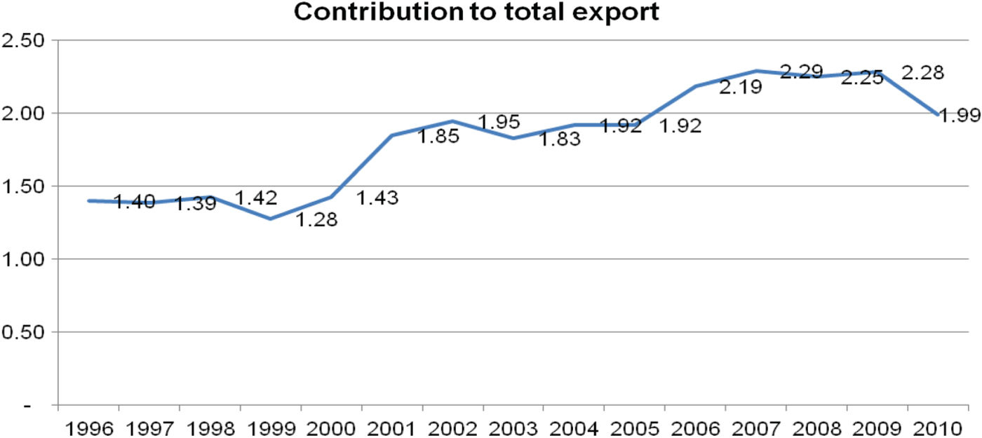
From 2007 to 2008, the global market value of EGS was GB£3,046bn, with Asia accounting for 38 per cent and India for 6.3 per cent (BERR, 2009).Footnote 1 In recent times, EGS production has emerged as a distinct industry in India.Footnote 2 For example, in 2003 the US Department of Commerce ranked the Indian EGS sector as the second most attractive sector after computer software services for US exporters and investors. The share of India's EGS in total exports rose from 1.4 per cent in 1996 to a peak of 2.28 per cent in 2009 (figure 1). However, despite the low effective tariffs on EGS in developed countries and in some developing countries (Mikic, Reference Mikic2010), trade and investment in EGS remain low. This is mainly due to ‘behind the border’ constraints such as weak infrastructure, institutions and non-tariffs barriers in many EGS-exporting countries, including India. In this context, then, the important questions are: has India fully achieved its export potential of EG? If not, how can India improve its EG export potential?
Contribution of EGS to total exports of India (%)

The paper is structured as follows. The next section describes the concept of EGS and provides an overview of India's exports of EG. Section 3 describes theoretical and empirical models, as well as data relating to EG. Section 4 discusses the results of estimation, together with the results of the decomposition of the changes in EG exports during the periods 1996–2000 and 2005–2010. The conclusions of this study and its policy implications are presented in section 5.
2. Overview of EG and Indian exports of EG
2.1. Issues with the definition
The definition of EGS has been a contentious issue in WTO negotiations. Why it this so? Different perceptions of which good can be called an environmental good and which service can be called an environmental service can be attributed to the following: multiple-end use; relativism; attribute disclosure; and ‘like’ products at the WTO (Balineau and de Melo, Reference Balineau and de Melo2011). For example, Hamwey et al., (Reference Hamwey, Hoffmann, Vikhlyaev and Vossenaar2003) contended that an EG is considered to be any equipment, material or technology used to address a particular environmental problem (goods for environmental management – GEM), or as a product that itself is ‘environmentally preferable’ (environmentally preferable product – EPP) to other similar products because of its relatively lesser or reduced negative effect on human health and the environment (Katti, Reference Katti2005). Another description of EGS is ‘goods and services which measure, prevent, limit, minimize or correct environmental damage’ (OECD/Eurostat, 1999).
The issue of classification of EG is important from a trade policy point of view because it will set clear parameters about the types of goods that are actually liberalized. Different approaches toward the identification of goods have been proposed by WTO members over the past few years in order to achieve multilateral liberalization of trade in EG. Of these, the OECD list of EG classification is the outcome of an effort by OECD and Eurostat to gauge the size of the environmental industry. As Steenblik (Reference Steenblik2005) pointed out: ‘The OECD's larger list was created deductively: starting from general categories based on the classifications in the environment industry manual, it added specific examples in order to produce an estimate of average tariffs on a previously undefined class of goods.’ The APEC list was created with the objective of obtaining more favorable tariff treatment for EG. These two lists became the reference points for the World Bank's ‘WB43’ list and the ‘friends-153’ list proposed by the Friend of Environmental Goods group, comprised of Canada, EU, Japan, Republic of Korea, New Zealand, Norway, Switzerland, Taiwan and the United States. The latter list has a wide-ranging coverage of 153 goods, and in 2007 the aim of reducing tariffs for these products emerged as the proposal at the center of WTO negotiations (Sugathan, Reference Sugathan2013).
Since none of the above lists provides complete coverage of EG, some workable definitions of EG have been adopted in empirical analyses. Currently, as the ‘friends-153’ list has become the core framework for WTO negotiations on EG, it is referred to as the ‘WTO 153’ list. Following the framework of WTO, EG can be classified into 12 groups: air pollution control; management of solid and hazardous waste and recycling systems; clean up or remediation of soil and water; renewable energy plant; heat and energy management; wastewater management and potable water treatment; EPPs based on end-use or disposal characteristics; cleaner or more resource efficient technologies and products; natural risk management; natural resources protection; noise and vibration abatement; and environmental monitoring, analysis and assessment equipment (Monkelbaan, Reference Monkelbaan2011).
2.2. India's exports of EGS
Although the sector that produces EGS was virtually non-existent in India two decades ago, India has been evolving into an exporter of, as well as a promising market for, EGS. The domestic environmental industry, however, is still highly disorganized and dominated by small-scale units. The environmental business is shared by a number of entities including equipment suppliers, system suppliers, engineering procurement and construction contractors, consultants and service providers (Katti, Reference Katti2005).
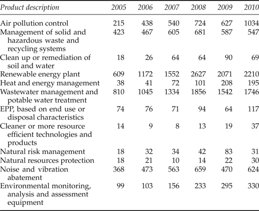
The contribution of EG exports has become increasingly important for India. Table 1 shows the export values of EG by groups over time. Before 2006, the group of ‘wastewater management and potable water treatment’ brought the highest value in terms of EG exports. However, the export of ‘renewable energy plant’ has played the most important role in the contribution of EG exports, accounting for more than US$2 trillion in 2010. The export of ‘air pollution control’ has also accrued high income for India, accounting for more than US$1 trillion in 2010.
India's exports of different categories of EG to the world (million US$)

According to recent data regarding India's exports of EG (WITS, 2013), the Asia-Pacific countries are important markets, with the value of India's EG exports to these markets increasing over time. The United States is a major importing partner that imports most of India's EG. For example, about 20 per cent of EG from the group ‘renewable energy plant’ was exported to the US market by India in 2010. In the same year, the values of India's goods sold to the United States in the groups ‘waste- water management and potable water treatment’ and ‘noise and vibration abatement’ were around US$300m and US$180m, respectively. In addition, China, Thailand, Malaysia and Australia are dominant importers of India's EG in the groups of ‘clean up or remediation of soil and water’ (China, US$10m; Malaysia, US$8m), ‘management of solid and hazardous waste and recycling systems’ (Thailand, US$34m) and ‘heat and energy management’ (Australia, US$35m).
3. Theoretical model and empirical strategy
3.1. Theoretical model
The gravity model (based on Newton's laws) is the most successful approach for empirically examining the factors affecting trade between countries. The model was first applied by Tinbergen (Reference Tinbergen1962), who found that the exports between two countries have a positive relation with GDP but a negative relationship with the geographic distance between countries. Although the gravity model has been criticized for its lack of theoretical underpinnings, many researchers (including Anderson, Reference Anderson1979; Bergstrand, Reference Bergstrand1989; Deardorff, Reference Deardorff and Frankel1998) have provided theoretical underpinnings for the gravity model. The basic gravity model can be written as:
 $$\eqalign{\hbox{Ln}\ E_{ij} & = \alpha + \beta_1 \hbox{Ln GDP}_i + \beta_2 \hbox{Ln GDP}_{j} + \beta_{3} \hbox{Ln POP}_{i} + \beta_{4} \hbox{Ln POP}_{j} \cr & \quad + \beta_{5}\ \hbox{Ln DIS}_{{ij}} + v_{ij}} $$
where Ln refers to natural logarithm; E ij refers to exports from country i to country j; GDP i is the gross domestic product of country i that may be interpreted as the ith country's productive capacity (supply side), while GDP j refers to that of the jth country; POP i denotes the size of the population of the ith country that may be interpreted as the consumption capacity (demand side), while POP j is that of the jth country; and DIS ij refers to the geographical distance between two major ports of countries i and j. The statistical error term ‘v ij ’ is the overall catch term for the remainder of the factors that influence trade between countries i and j. This error term is erroneously assumed to be distributed randomly, without any important influence on trade between countries. This is restrictive, as country-specific constraints such as infrastructural and institutional frameworks play crucial roles in determining trade relations between countries. These country-specific constraints are named in the literature as ‘behind the border’ constraints that exist in the exporting country, and ‘beyond the border’ constraints that exist in the importing country. These constraints, for example, concern port and customs procedures, patent licensing, banking procedures and transportation facilities.
Many studies have tried to improve the basic gravity model. For example, Matyas (Reference Matyas1998) showed that there are some omitted variables in the basic model, including exchange rates and foreign currency reserves. The author also proved that current exports and those of the previous year were highly related. Further, Anderson and Wincoop (Reference Anderson and Wincoop2001) argued that the conventional ordinary least squares estimation may suffer from omitted variables bias, and that the comparative statics analysis would be unfounded. Another problem of the gravity model with respect to the omitted variables concerns the exclusion of trade resistances such as non-tariff barriers from the gravity equation. To deal with these problems, researchers suggested different methods of modeling and estimation of the gravity equation. For example, some suggested fixed effects models (Bayoumi and Eichengreen, Reference Bayoumi, Eichengreen, Ito and Krueger1997), while Egger and Pfaffermayr (Reference Egger and Pfaffermayr2003) suggested the use of panel data models that are non-linear in trade costs, and Feenstra (Reference Feenstra2002) used price differences between trading partners in his specification of the gravity model. Since McCallum (Reference McCallum1995), many empirical papers have used ‘remoteness’ variables, generally defined by
 $\sum_{m \ne j} \displaystyle{{d_{im}} \over {y_m}}$
, where d is distance and y is GDP, and the whole term represents the weighted average distance of country i from all its trading partners, except the particular partner j. Anderson and Wincoop, (Reference Anderson and Wincoop2001) criticized these remoteness variables and suggested another multilateral resistance term. The multilateral resistance term implies that when we observe no movement in the trade determinants between country i and country j, but do observe a change in country k's trade with country i, then this will affect trade between countries i and j. However, Anderson and Wincoop assumed symmetrical trade costs to solve their model, which is an unrealistic assumption. Thus, the above solutions are either not based on any theoretical arguments or cannot fully capture the inherent bias in the empirical estimation. These solutions have also given biased results due to ignoring heteroskedasticity and non-normality of the error term of the gravity equation, which emanate from the omitted variables bias.
Kalirajan (Reference Kalirajan2008) suggested an alternative methodology to model and estimate the gravity model by taking into account the country-specific constraints related to trade, which have bearings on heteroskedasticity and non-normality of the error term, and which draw on the modeling and estimation procedures used in the stochastic frontier production function literature. The advantage of using the stochastic frontier gravity model is that it is possible to incorporate and measure the effects of country-specific ‘behind the border’ and ‘beyond the border’ constraints on exports when the researcher does not have full information about these constraints.Footnote 3 The stochastic frontier gravity model that incorporates the overall impact of ‘behind the border’ and ‘beyond the border’ constraints along with the conventional determinants of exports can now be written as follows:
 $$\eqalign{\hbox{Ln} E_{ij} &= \alpha + \beta_{1} \hbox{Ln GDP}_{i} + \beta_{2} \hbox{Ln GDP}_{j} + \beta_{3} \hbox{Ln POP}_{i} + \beta_{4} \hbox{Ln POP}_{j} \cr & \quad + \beta_{5} \hbox{Ln DIS}_{ij} - u_{ij} + v_{ij}} $$
It is assumed that u ij is zero if the influence of overall ‘behind the border constraints’ is not significant; otherwise, it takes a positive value. u ij is assumed to follow a truncated normal distribution, truncated at zero, and v ij is assumed to represent the ‘beyond the border’ constraints and other left-out variables including statistical errors. It is assumed to follow a full normal distribution with mean zero and a constant variance.
Now, export potential is defined as the maximum possible exports that can be achieved in contrast to the average exports that are often estimated using the conventional gravity model analysis. Export potential can be used as an estimate of what exports would be in the hypothetical case of most frictionless and free trade that is possible under present circumstances observed in all India's trade partners. Export performance, therefore, is a measure that consists of the ratio of actually realized level of exports to potential exports, and the latter can be estimated by using the stochastic frontier gravity model for export flows. This measure is relevant in the present context of examining the impact on the export performance of the exporting country, not only of its trade policy reforms, but also of the importing countries. In addition, export performance is not only affected by policies that promote or limit the exchange of goods and services, but also by infrastructure and institutions that facilitate or inhibit trade and investment between countries. Hence, it is useful from a policy perspective to identify the factors that contribute to a country's export performance, and this is attempted in the following paragraphs.
Following Kalirajan (Reference Kalirajan2008), export growth can be decomposed in terms of different components of the determinants of export growth, such as ‘natural’ determinants, ‘behind the border’ determinants, and ‘beyond the border’ determinants, where the latter can be divided further into ‘explicit beyond the border’ and ‘implicit beyond the border’ determinants. Thus, the export of EG depends on many factors. First, it depends on the GDP and population of importing countries. The assumption is that higher GDP and population in the foreign countries would generally lead to an increase in demand for EG from India. However, the relationship between distance and EG exports is negative due to the higher cost of transportation. These factors can be termed ‘natural’ determinants of export flows between countries.
Next, ‘explicit beyond the border’ determinants such as the relative price of the imported goods and services that are mainly influenced by importing countries' tariff and exchange rates are other factors affecting export performance. These determinants are expected to have a negative correlation with EG exports because increasing tariffs and the devaluation of domestic currencies lead to higher imported prices in the domestic market. Hence, the demand for imports is reduced.
Different kinds of institutional and infrastructural rigidities that exist in the exporting countries, such as poor port facilities, may influence exports negatively. These factors may be referred to as ‘behind the border’ determinants in the home country, which are under the control of the exporting countries. The ‘behind the border’ determinants in the case of EG exports mostly include license and market access restrictions, restrictions on foreign equity and joint venture partners, a legal system with limited effectiveness in terms of enforcement, and limited protection of intellectual property rights. For example, one of the major ‘behind the border’ constraints in the case of wind turbine exports is the lack of international standards for certification and approval, with the issue of differing standards effectively becoming a major trade barrier (Alavi, Reference Alavi2007). Thus, a lack of knowledge about the different types of non-tariff barriers such as the above that exist in partner countries is an important ‘behind the border’ constraint in exporting countries.
Unfortunately, the researchers were unable to quantify all the ‘behind the border’ determinants individually. Nevertheless, the combined effects of all of these determinants can be modeled as a random variable with a truncated normal distribution.
Also, different kinds of institutional and infrastructural rigidities that exist in the importing countries can influence export flows negatively. These factors may be called ‘implicit beyond the border’ determinants that are beyond the control of the exporting countries. This is modeled as a random variable with a full normal distribution.
Free trade agreements (FTA) that are in the form of improvement in the trade promotion and facilitation policies of both India and its trading partners are expected to positively influence Indian EG exports. A dummy variable (TA) can be used to represent whether there are such trade agreements and the influence of these factors on exports may be called ‘mutually induced’ determinants.
India's export potential of EG with respect to its individual trading partners in a particular time period can be calculated by multiplying the estimated coefficients of the model (2) with the actual values of the determinants of exports used in the same model, with the assumption that
 $u_{{ij}}$
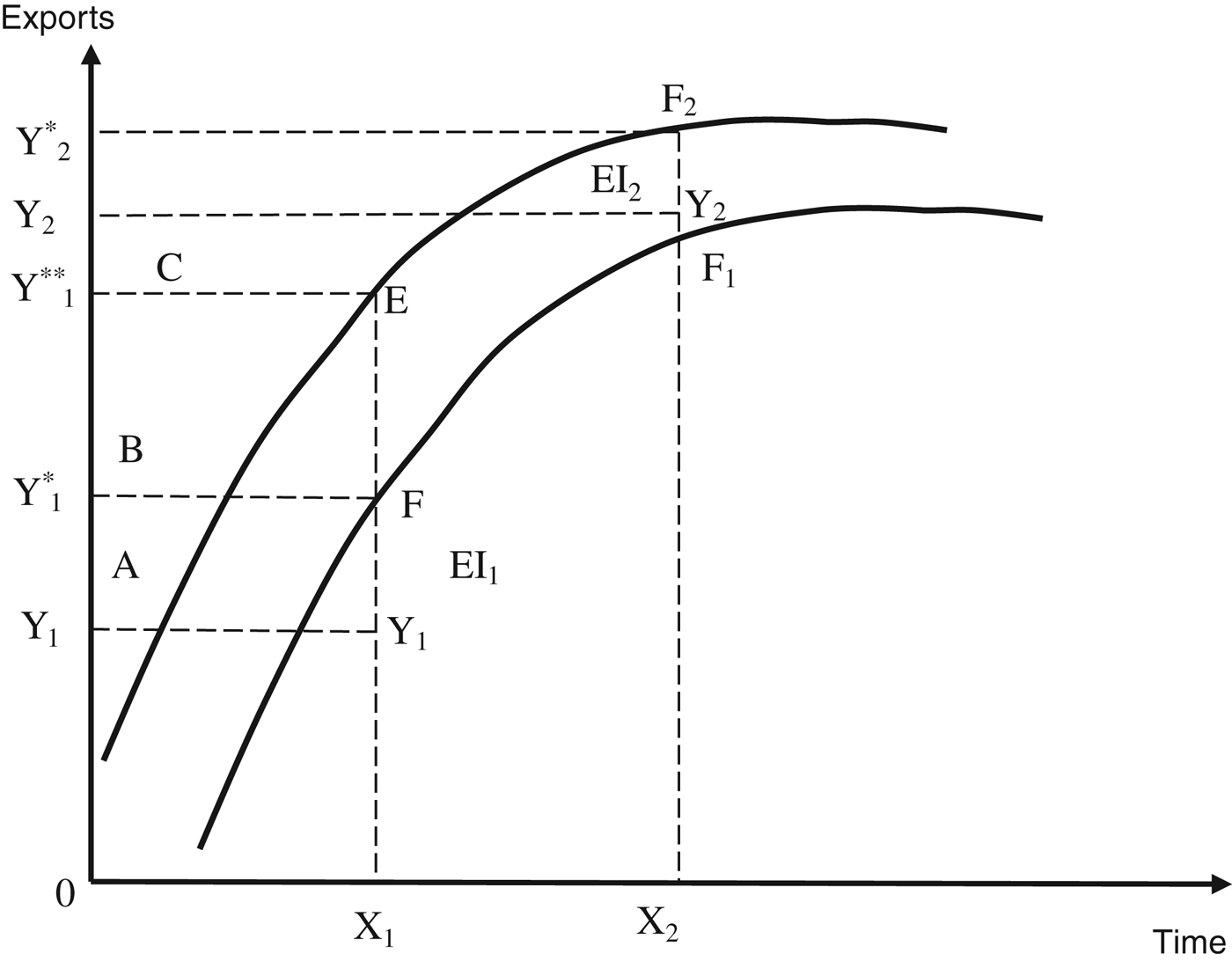
is zero, indicating that there are no ‘behind the border’ constraints in India. The difference between such potential exports between two time periods denotes the change in India's potential exports with respect to the concerned trading partner. The methodology for decomposing the changes in exports between two time periods is explained in figure 2. F
1 is the potential export frontier of the home country in period 1 and in the absence of any ‘behind the border’ constraints; Y
1* in period 1 is called potential exports for the given export determinants, say, X
1. The actual export is Y
1, which is less than Y
1* due to the existence of ‘behind the border’ constraints emanating from infrastructure constraints, institutional rigidities and other similar weaknesses in the home country. EI
1 is the export inefficiency resulting from ‘behind the border’ constraints, which prevents the export in period 1 from reaching its potential. EI
1 is measured as the vertical distance between actual exports and potential exports for the given export determinants X
1. However, ‘implicit beyond the border’ constraints tend to change due to multilateral or bilateral negotiations or trade facilitation steps taken by the partner countries. These would generally shift the potential export frontier from F
1 to F
2 in period 2. Nevertheless, while Y
2* represents the potential exports without any ‘behind the border’ constraints in the home country, Y
2 is the actual exports, which is less than Y
2* due to the existing ‘behind the border’ constraints in the home country in period 2. Potential exports growth due to reduction in ‘implicit beyond the border’ constraints can be measured as the vertical distance between the frontier in period 1 (Y
1*) and the frontier in period 2 (Y
1**) evaluated for the same levels of determinants of exports, X
1 in period 1. This is calculated first by multiplying the actual levels of determinants of exports in period 1 by their relevant estimated frontier coefficients of period 2 and, secondly, taking the difference between this calculated export level and the potential export of period 1.
Export growth decomposition

The change in realized exports can be decomposed (figure 2) as follows (Khan and Kalirajan, Reference Khan and Kalirajan2011):
 $$\eqalign{D &= Y_{2} - Y_{1} = A + B + C \cr &= [ Y_{1}^{\ast} - Y_{1}] + [ Y_{1}^{\ast \ast} - Y_{1}^{\ast}] + [ Y_{2} - Y_{1}^{\ast \ast}] \cr &= [ Y_{1}^{\ast} - Y_{1}] + [ Y_{1}^{\ast \ast} - Y_{1}^{\ast}] + [ Y_{2}^{\ast} - Y_{1}^{\ast \ast}] - [ Y_{2}^{\ast} - Y_{2}] \cr &= \lcub [ Y_{1}^{\ast} - Y_{1}] - [ Y_{2}^{\ast} - Y_{2}] \rcub + [ Y_{1}^{\ast \ast} - Y_{1}^{\ast}] + [ Y_{2}^{\ast} - Y_{1}^{\ast \ast}] \cr &= \lcub {EI}_{1} - {EI}_{2}\rcub + \hbox{CIBBC} + \hbox{GCD}} $$
where EI 1 − EI 2 = the difference between export inefficiency in period 1 and period 2 resulting from changes in ‘behind the border’ constraints in exporting country (BTBC); CIBBC = change in exports due to the trade facilitation steps taken by the partner countries, leading to changes in ‘implicit beyond the border’ constraints (IBTBC); GCD = change in exports due to the sum of changes in the core natural determinants of trade (CD) such as GDP and population, changes in ‘mutually induced’ determinants such as trade agreements, and changes in ‘explicit beyond the border’ constraints (EBTBC), which include tariffs and exchange rates.
Thus, the changes in exports between two periods may result from: the reduction in ‘behind the border’ constraints over time through the exporting country's domestic reforms; the reduction in both ‘explicit and implicit beyond the border’ constraints in partner countries due to partner countries' reforms and mutual discussions; the increase in export demand in partner countries due to increase in partner countries' GDP levels and population; and the implementation of trade agreements between home and partner countries.
3.2. Empirical strategy
The empirical stochastic frontier gravity model used in this study is:
 $$\eqalign{\hbox{Ln}\lpar X_{ijk}\rpar & = \alpha_{1} + \alpha_{2} \hbox{ln}\lpar \hbox{GDP}_{j}\rpar + \alpha_{3}\hbox{ln}\lpar \hbox{POP}_{j}\rpar + \alpha_{4} \hbox{ln}\lpar \hbox{DIST}_{ij}\rpar + \alpha_{5} \hbox{Ln}\lpar \hbox{EXR}_{ij}\rpar \cr & \quad + \alpha_{6} \hbox{Ln}\lpar \hbox{T}_{ijk}\rpar + \alpha_{7} \hbox{Ln}\lpar \hbox{TA}_{ij}\rpar - u_{ij} + v_{ij}\comma \; }$$
in which X ijk describes India's exports of the kth group of EG to country j; GDP j and POP j measure the GDP and population of the importing country j; DIST ij indicates the distance from New Delhi to the capital city of the India's partner country j; EXR ij is the nominal exchange rate of local currency of India's trading partners and is in US dollars; T ijk is the average tariff levied on India for the kth group of EG by the importing country j; TA ij is a dummy variable, which is equal to 1 if the importing country j had a trade agreement with India, otherwise 0; u ij refers to the combined effect of ‘behind the border’ constraints in India with respect to the importing country j,Footnote 4 and v ij is the ‘normal’ statistical error term and implicit ‘beyond the border’ constraints. It is assumed that u ij is zero if the influence of ‘behind the border’ constraints is not significant; otherwise it takes a positive value. u ij is assumed to follow a truncated normal distribution, truncated at zero, and v ij is assumed to follow a full normal distribution with mean zero and a constant variance. Using the joint density functions of u ij and v ij , the maximum likelihood estimation can be used to estimate the production coefficients, α1… α7 along with the total variance and the parameter γ, which is the ratio of the variance due to the combined effect of ‘behind the border’ constraints to total variance of exports. Thus, γ indicates whether ‘behind the border’ constraints are one of the determinants of total exports of EG, and also serves as a robustness test for the gravity model given in (2). When γ is significant, it means that ‘behind the border’ constraints are important determinants of EG exports. The software FRONTIER 4.1 (Coelli, Reference Coelli1996) is used to estimate the above model (4) for four different years, 1996, 2000, 2005 and 2010.Footnote 5
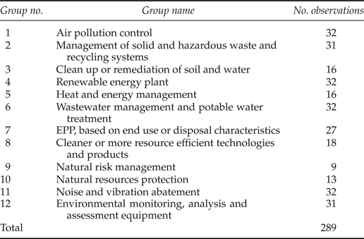
EG used in this study were taken from the WTO 153 list, which is divided into 12 groups. Given the importance of the Asia-Pacific countries for India's EG exports, the top 10 Asia-Pacific markets were considered for empirical analysis in this study. These countries include Australia, Canada, China, Indonesia, Japan, Malaysia, Republic of Korea, Singapore, Thailand, Vietnam, and the United States. The data on exports of EG from India were collected from the official website of World Integrated Trade Solution (WITS) for the period 1996–2010, while GDP, population and exchange rate were derived from the official website of the World Bank (WB). The data on distance were calculated between capital cities in India and its partner countries using the Distance Calculator website. Tariff data were extracted from WITS by HS 6-digits, with tariffs calculated by averaging tariffs for 12 groups of EGS. Trade agreements were collected from the website of the Ministry of Commerce and Industry of India. The data consist of cross-country balanced data for four years, which means that four-year samples used for the estimations are identical in terms of India's trade partners for each EG category. Sample size by EG export categories is given in table 2, which shows 289 observations in 1996, 2000, 2005 and 2010.
Sample size: India's exports by EG categories to its selected partner countries

4. Results of estimation and decomposition of changes in India's exports of EG
4.1. Results of estimation
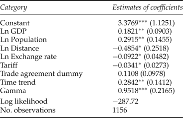
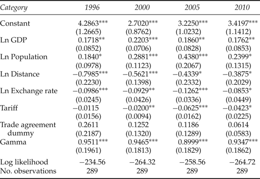
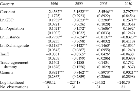
The estimated results of the determinants of India's total exports of EG are shown in table 3. The high value of γ, which varies from 0.90 to 0.95 at the 1 per cent level of significance, confirms that the selected stochastic frontier gravity model framework (equation (4)) for the present study is statistically valid for the present data set. It also shows that the variation of India's exports of EG mostly comes from the inefficiency emanating from ‘behind the border’ constraints. This implies that India has to eliminate its ‘behind the border’ constraints by improving its infrastructure and institutions to increase its EG exports.
Maximum likelihood estimates of the stochastic frontier gravity model in the panel data framework

Notes: Dependent variable: India's total exports of EG in logarithm.
Figures in parentheses are standard errors of estimates.
***, **, * show the significance level at 1%, 5%, and 10%, respectively.
All the coefficients vary over time during the period 1996–2010, which indicates that the influence of different types of determinants of EG exports has also been changing over time. As a kind of sensitivity analysis to prove the robustness of the estimated results, the stochastic frontier gravity model was estimated in the panel data framework using FRONTIER 4.1 software. The results are given in table 3.Footnote 6 The interesting result of the panel data estimation is that the coefficient of the time trend is significant at the 5 per cent level, which confirms the individual year estimation results of variation of coefficients given in table 4.
Maximum likelihood estimates of the stochastic frontier gravity model

Notes: Dependent variable: India's total exports of EG in logarithm.
Figures in parentheses are standard errors of estimates.
***, **, * show the significance level at 1%, 5% and 10%, respectively.
The results in table 4 show that the coefficients of GDP are positive, at least at the 5 per cent significance level. The coefficients first increased from 0.1718 in 1996 to 0.2203 in 2000, and then declined to 0.1762 in 2010. This shows that during the period 1996–2000 the GDP of partner countries had an increasingly positive effect on India's EG exports, while in later periods the impact was smaller. There may be many reasons for that. For example, as India's trading partners' GDP increases, they may produce import-substituting EG, which then would reduce the imports from India.
The coefficients of exchange rate have negative signs as expected, with a significance of at least 10 per cent in 2010. This means that when India's partner countries depreciate their currencies, the prices of EG imported from India are relatively more expensive. Consequently, the demand for India's EG is reduced. This factor is not under India's control and belongs to ‘explicit beyond the border’ constraints.
Tariff is another crucial factor in determining India's exports of EG. While tariff had no effect on EG exports from India in 1996, it significantly and negatively influenced EG exports in 2000. Since then, the coefficient of tariff has become significant and on a declining trend from 2005 until recently. This indicates the effectiveness of reducing the ‘explicit beyond the border’ constraints by India's trading partners through implementing their trade policy reforms to reduce trade costs to benefit their importers. Such policy measures also benefit EG-exporting countries, including India.
The coefficient of trade agreement is not significant during the sample periods. Thus, trade agreements, which do not specifically involve EG and are mostly in the form of either reduced or zero tariffs, do not appear to be effective in promoting India's EG exports. This may be explained by observing the actual export activities of India. For example, while there is no trade agreement between India and the United States, the value of India's export of EG to the United States accounted for 20 per cent of total EG exports in 2010. Also, as discussed above, a reduction in ‘explicit beyond the border’ constraints by India's trading partners has the potential to make tariff less important to India's EG export growth.
4.2. Results of decomposition of changes in India's exports of EG
Changes in India's EG exports are decomposed for the selected 10 Asia-Pacific economies that were major trading partners of India for EG for the two periods 1996–2000 and 2005–2010.
The decomposition of the output growth of EG for each trading partner of India is accomplished by working through the following steps:
-
(i) the actual export growth between 2000 and 1996 is calculated as (Y 2 − Y 1) given in equation (3);
-
(ii) the difference between the estimated frontier exports (Y 1*) and the actually realized output (Y 1) in year 1996 is calculated, which is named as EI 1 given in (3);
-
(iii) the difference between the estimated frontier exports and the actually realized output in year 2000 is calculated, which is named as EI 2 given in (3);
-
(iv) frontier export, Y 1** given in (3) is obtained by multiplying the actual levels of the determinants of exports of 1996 by the 2000 estimates of the frontier coefficients;
-
(v) the difference between Y 1** and Y 1* is calculated, which is named as the change in export growth due to the changes in ‘implicit beyond the border’ constraints in the partner countries;
-
(vi) the difference between EI 1 and EI 2 is calculated, which is named as the change in export growth due to the changes in ‘behind the border’ constraints in India; and
-
(vii) the differences calculated in steps (vi) and (vii) are added together and this amount is then subtracted from (Y 2 − Y 1) to get (Y 2* − Y 1**) given in (3), which is named as the change in exports due to the sum of changes in ‘explicit beyond the border’ constraints and in the core natural determinants of exports such as GDP and population.
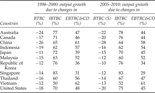
The results thus obtained in the above steps of (vi), (vii), and (viii) are presented as percentages of output growth in table 5. Similar calculations were carried out for the output growth between 2005 and 2010, and the results are presented in table 5.
India's EG exports growth decomposition for 1996–2000 and 2005–2010

Notes: BTBC, behind the border constraints; IBTBC, implicit beyond the border constraints; EBTBC&CD, explicit beyond the border constraints and core determinants.
(+) A positive sign for BTBC would have meant that there was a reduction in the ‘behind the border’ constraints in India between the relevant periods of analysis; (−) a negative sign for BTBC means that there is no reduction in the ‘behind the border’ constraints in India between the relevant periods of analysis.
Table 5 shows that, in most cases, the ‘behind the border’ constraints that are under the control of India have negative effects on India's EG exports growth, while the reduction of the ‘implicit beyond the border’ constraints that are under the control of India's trading partners have contributed strongly positively to the EG exports growth. For example, the ‘behind the border’ constraints in India contributed to the decline of EG export growth to Australia during the periods 1996–2000 and 2005–2010 by 24 and 22 per cent, respectively. However, India's EG exports growth to Australia was influenced more by the reduction in the ‘implicit beyond the border’ constraints implemented by Australia than by increased demand arising from increased GDP and population. The case with all the other countries shown in table 5 is similar. Thus, these results indicate that India should implement serious reform measures to eliminate its ‘behind the border’ constraints.
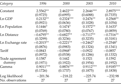
As the above analysis concerns the decomposition of exports growth of total EG, it may be interesting to see the decomposition of exports growth of individual categories of EG in order to understand whether the determinants and decomposition of exports growth of individual categories differed across categories. Two major product groups – ‘environmentally preferable products’ and ‘environmental monitoring, analysis and assessment equipment’, which represents the GEM category – are taken for further analysis in this paper.Footnote 7 The results of the estimation of the determinants of EPP are given in table 6. Both the size and significance of the γ coefficient imply that the estimated stochastic frontier gravity model is appropriate to gauge the determinants of exports growth of EPP. It is worth noting that there is not much difference between the determinants of EPP exports and total EG exports during the periods of analysis. Table 7 shows the results of estimation of determinants of the GEM category ‘environmental monitoring, analysis and assessment equipment’.
Maximum likelihood estimates of the stochastic frontier gravity model

Notes: Dependent variable: India's exports of EPP in logarithm.
Figures in parentheses are standard errors of estimates.
***, **, * show the significance level at 1%, 5% and 10%, respectively.
Maximum likelihood estimates of the stochastic frontier gravity model

Notes: Dependent variable: India's environmental monitoring, analysis and assessment equipment (GEM category) exports in logarithm.
Figures in parentheses are standard errors of estimates.
***, **, * show the significance level at 1%, 5% and 10%, respectively.
The significance of the γ coefficient indicates that the selected model is appropriate to explain the influence of the selected determinants on exports. The determinants of this GEM category appear not to differ sufficiently from the determinants of EPP and the total EG exports. Now, the decomposition of both EPP exports growth and GEM category exports growth are carried out following the methods described above, and the results are given in tables 8 and 9, respectively. The results can be summarized as follows.
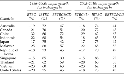
Exports growth decomposition for 1996–2000 and 2005–2010: India's EPP, based on end use or disposal characteristics

Notes: BTBC, behind the border constraints; BTBC, implicit beyond the border constraints; EBTBC&CD, explicit beyond the border constraints and core determinants.
(+) A positive sign for BTBC would have meant that there was a reduction in the ‘behind the border’ constraints in India between the relevant periods of analysis; (−) a negative sign for BTBC means that there is no reduction in the ‘behind the border’ constraints in India between the relevant periods of analysis.
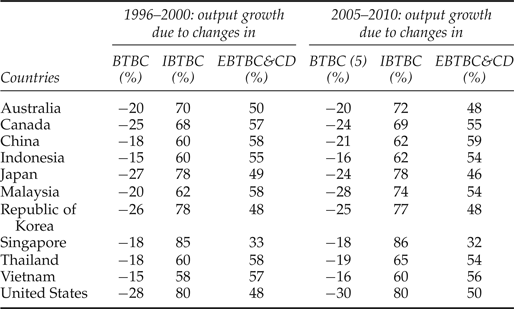
Exports growth decomposition for 1996–2000 and 2005–2010: India's environmental monitoring, analysis and assessment equipment exports

Notes: BTBC, behind the border constraints; BTBC, implicit beyond the border constraints; EBTBC&CD, explicit beyond the border constraints and core determinants.
(+) A positive sign for BTBC would have meant that there was a reduction in the ‘behind the border’ constraints in India between the relevant periods of analysis; (−) a negative sign for BTBC means that there is no reduction in the ‘behind the border’ constraints in India between the relevant periods of analysis.
4.2.1. Environmentally preferable products
India's exports of EPP (table 8) were substantially negatively influenced by the export inefficiency arising from the ‘behind the border’ constraints in both periods. On the other hand, the large reductions in the ‘implicit beyond the border’ constraints in India's partner countries arose from either bilateral/multilateral negotiations or trade facilitation measures taken by them in both periods. In contrast, the contribution of the reduction in ‘explicit beyond the border’ constraints to India's export growth of this EG group was relatively small during the period 2005–2010.
4.2.2. Environmental monitoring, analysis and assessment equipment
As observed with respect to the EPP exports growth, the effect of the ‘behind the border’ constraints was significant for India's export growth of this GEM group of ‘environmental monitoring, analysis and assessment equipment’ during the period 1996–2000 (table 9). However, the reductions in the ‘implicit beyond the border’ constraints dominated and positively contributed to India's export growth of this GEM group of EG in the next period. Nevertheless, for example, although the reduction in Malaysia's ‘implicit and explicit beyond the border’ constraints caused a 14 percentage point increase in India's exports of EG of the GEM group to Malaysia from the first period (1996–2000) to the second period (2005–2010), India's institutional and infrastructure rigidities reduced Malaysia's imports by 8 percentage points during the same periods. Consequently, India's exports of EG of ‘environmental monitoring, analysis and assessment equipment’ group to Malaysia declined significantly during the period 2005–2010 from its potential level.
Thus, the above analyses indicate that the sources of EG exports growth at the aggregate level appear to be similar. However, at the individual product group level, there seem to be slight differences. For example, EPP exports appear to be more influenced by ‘behind the border’ constraints and local demand in importing countries than the GEM exports, though the latter is more sensitive to ‘distance’.Footnote 8 It would be interesting to know why this is so. Some conjectures can be made: regulation on environmental standards and the need for environmental certifications are some of the crucial non-tariff barriers to EG trade (Khatun, Reference Khatun2010). The inability of India's EG exports to meet the high standards imposed by the importing country will be reflected in the size of γ, which implies the influence of the ‘behind the border’ constraints on exports. Further, there are no uniform environmental requirements and technical regulations across countries, which means that local demand for the type of EG used to meet environmental requirements varies from country to country. Therefore, it is logical to argue that a significant increase in EG trade will require more than just zero tariff (Cosbey, Reference Cosbey2011).
5. Conclusions
EG can bring more benefit to the Indian economy in increasing its national income through exports. A stochastic frontier gravity model is used to examine whether India has achieved its EG export potential with its top 10 export markets of the Asia-Pacific economies, using the WTO 153 list classified into 12 groups. The advantage of using the stochastic frontier gravity model is that it is possible to incorporate country-specific ‘behind the border’ and ‘beyond the border’ constraints into the conventional gravity model to estimate their impacts on India's exports of EG. In this context, researchers did not need to have detailed information on ‘behind the border’ and ‘beyond the border’ constraints, as these constraints are represented as independently distributed random variables with different distributional functions. The analysis was carried out for the four years 1996, 2000, 2005 and 2010. The results show that the contributions of GDP of partner countries have a positive effect, while the distance between India and its trading partners, exchange rate and tariffs have negative effects on the exports of India's EG. Next, the changes in India's exports of EG were decomposed into different components, such as growth due to reductions in ‘behind the border’, ‘implicit beyond the border’ and ‘explicit beyond the border’ constraints, along with ‘natural’ determinants and ‘mutually induced policy’ determinants. The results show that the institutional and infrastructure rigidities of India, which are the main causes of the emergence of ‘behind the border’ constraints, exert dominant negative effects on its exports of EG to India's trading partners in the Asia Pacific. On the other hand, the reduction in India's trading partners' ‘implicit beyond the border’ constraints made a significant contribution to India's EG exports growth during the period 1996–2010. The export growth changes due to ‘explicit beyond the border’ constraints are relatively small. Thus, these results, which hold good whether the analysis is done at the aggregate total EG exports level or individual EG categories level, indicate to India that it should eliminate its ‘behind the border’ constraints.
Therefore, in terms of policy suggestions to promote exports of EG, India needs to strengthen its policies to remove ‘behind the border’ constraints to improve its infrastructure and institutional framework, which are central to India's exports. Due to a lack of uniform data, we could not identify ‘behind the border’ constraints; however, some evidence-based conjectures can be made. For example, India can improve the performances of its exporting firms by disseminating knowledge and laws related to EG of the importing countries. Further, port facilities can be improved so that they function efficiently, and bureaucratic delays in dispatching EG can be avoided. With respect to the advanced technology involved in the production of EG, Lema and Lema, (Reference Lema and Lema2012) have argued that conventional technology transfer mechanisms such as FDI, patent licensing and imports are crucial. In this context, it is well known that India's FDI policy has been very restrictive until recently (Sahoo et al., Reference Sahoo, Nataraj and Dash2013), which has been an institutional rigidity influencing EG export growth negatively.
A limitation of this study concerns the following. The impact of the changes in ‘implicit beyond the border’ constraints to India's exports of EG is measured by the vertical distance between the frontier in period 1 and the frontier in period 2, evaluated for the same level of determinants of exports for period 1. This impact may also include the changes in the price of EG which lead to changes in the value of Y 1**. As appropriate data were unavailable, this study does not separate the effects of the changes in prices, statistical and measurement errors, and other omitted variables from the impact of ‘implicit beyond the border’ constraints.