


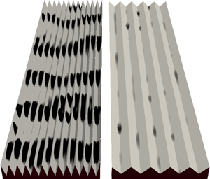


1. Riblets and Kelvin–Helmholtz rollers
Riblets are streamwise-aligned surface grooves with design sizes of the order of  $10$ viscous units that have the potential to reduce skin-friction drag compared to a smooth wall. They are classified as passive flow-control devices, as no energy input is required to favourably alter the flow field, making them attractive for aeronautical (Szodruch Reference Szodruch1991) and maritime (Letcher et al. Reference Letcher, Marshall, Oliver and Salvesen1987) applications as well as for pipes (e.g. Liu et al. Reference Liu, Christodoulout, Ricciust and Joseph1990; Peet, Sagaut & Charron Reference Peet, Sagaut and Charron2009). The design of riblets builds on the idea by Kramer (Reference Kramer1937) for streamwise-aligned wires that shield a surface below from drag-increasing turbulence. Early experimental results by Liu, Kline & Johnston (Reference Liu, Kline and Johnston1966) suggested the possibility of drag reduction by riblet surfaces and Walsh et al. investigated drag characteristics of different riblet geometries at varying flow conditions (e.g. Walsh & Weinstein Reference Walsh and Weinstein1978; Walsh Reference Walsh1982). Roughly half of the drag transport aircraft experience in cruise conditions results from skin-friction drag (e.g. Schrauf Reference Schrauf2005), making its reduction financially and environmentally attractive. Laboratory tests of riblets have reduced skin-friction drag by up to 8.2 % for friction Reynolds numbers
 ${Re_\tau \equiv \delta u_\tau / \nu \lesssim 700}$ (Bechert et al. Reference Bechert, Bruse, Hage, van der Hoeven and Hoppe1997), where
 $\delta$ is the half-channel height,
 $\nu$ the kinematic viscosity and
 ${u_\tau \equiv \sqrt {\tau _w/\rho }}$ the friction velocity defined with the density
 $\rho$ and the wall-shear stress (drag per unit plan area)
 $\tau _w$. Following Spalart & McLean (Reference Spalart and McLean2011), this reduction in skin-friction drag scales to approximately 5.5 % for flight conditions at
 ${Re_\tau }\approx 48\,000$ and it is only marginally affected by yawed flow up to angles of
 $15^{\circ }$ (Walsh & Lindemann Reference Walsh and Lindemann1984). Possible applications explain ongoing interest by the aircraft industry and continued effort to overcome practical challenges (e.g. Bilinsky Reference Bilinsky2019; Linde & Hegenbart Reference Linde and Hegenbart2019).
Drag reduction by riblets relative to a smooth wall at matched  ${Re_\tau }$ is defined as
 ${{DR} \equiv 1-C_f/C_{f,{smooth}}}$. The skin-friction coefficient
 $C_f=2/U^{+2}_{\delta }$ is determined by the viscous-scaled mean streamwise velocity
 $U^{+}=U/u_\tau$ evaluated at the half-channel or boundary-layer height
 $\delta$. The superscript
 $+$ is used to denote viscous scaling with
 $\nu$ and
 $u_\tau$ throughout this paper. For small differences in drag between the two surfaces,
 ${{DR}\propto -{\rm \Delta} U^{+}}$, where
 ${{\rm \Delta} U^{+} \equiv U^{+}_{{smooth}}-U^{+}}$ is the shift between the profiles of mean streamwise velocity for the smooth and riblet surfaces at matched height in or above the logarithmic layer. Unlike a fractional drag change,
 ${\rm \Delta} U^{+}$ is independent of the Reynolds number for large
 ${Re_\tau }$ and low blockage (Spalart & McLean Reference Spalart and McLean2011). In figure 1(a) we observe that the drag change
 ${\rm \Delta} U^{+}$ depends strongly on the riblet size, which we measure using the viscous-scaled square root of the groove cross-sectional area
 $\ell _g^{+}$ as proposed by García-Mayoral & Jiménez (Reference García-Mayoral and Jiménez2011b). Small riblets repel turbulent eddies by obstructing their induced spanwise flow and thus reduce mixing of streamwise momentum and consequently skin-friction drag. The detailed description of the flow around riblets that explains drag reduction mainly comes from various works of Bechert et al. and Luchini et al. and was recently reviewed by García-Mayoral, Gómez-de-Segura & Fairhall (Reference García-Mayoral, Gómez-de-Segura and Fairhall2019). Luchini et al. (Reference Luchini, Manzo and Pozzi1991) explain the drag-reduction mechanism for riblets that are small enough for the flow around them to be dominated by viscosity, which is therefore described by Stokes flow. In this framework, the cross-flow from quasi-streamwise vortices is represented by spanwise Stokes flow
 $v_r$ (figure 1b), which penetrates the groove to a depth below the crest given by the lateral protrusion height
 $\ell _v$. Importantly, this is less than the protrusion height of streamwise Stokes flow
 $\ell _u>\ell _v$. In turbulent flow, the penetration depth of Reynolds stresses given by
 $\ell _T \sim \ell _v$ is thus less than the streamwise protrusion height
 $\ell _U>\ell _T$ (Luchini Reference Luchini1996). If we now consider a reference smooth wall
 $\ell _T$ below the riblet crest, both flows are similar (Luchini Reference Luchini1996) in that their total stresses match at every height. The origins of streamwise flow of the two surfaces, however, differ by
 $\ell _U - \ell _T = \ell _u - \ell _v>0$ in the Stokes-flow limit. That difference describes the velocity decrement
 ${\rm \Delta} U^{+}\approx \ell ^{+}_T - \ell ^{+}_U < 0$, because both riblet and smooth-wall velocity profiles have the same slope
 $\mathrm {d}U^{+}/\mathrm {d}z^{+} \approx 1$ in the viscous sublayer (Luchini Reference Luchini1996). Consequently,
 $U^{+} \approx U^{+}_{{smooth}} - {\rm \Delta} U^{+}$ at every height above the reference smooth wall. In the Stokes-flow limit, riblet geometries with sharp tips (triangular and parabolic grooves) have a higher protrusion height difference than rounded sinusoidal profiles (Luchini et al. Reference Luchini, Manzo and Pozzi1991). However, the protrusion height difference of finite-thickness blade riblets increases through tip rounding, because it effectively sharpens the otherwise flat tips (García-Mayoral & Jiménez Reference García-Mayoral and Jiménez2011a). The theoretical maximum
 $\ell _u - \ell _v \approx 0.13s$, where
 $s$ is the riblet spacing, is attained for infinitely thin (sharp) and deep blade riblets (Luchini et al. Reference Luchini, Manzo and Pozzi1991). Viscous analysis further predicts a linear decrease of drag for small riblets (straight lines in figure 1a), which implies that drag reduces with increasing riblet size until they are large enough that inertial effects contribute to momentum transport in the vicinity of the wall. For larger riblets therefore, viscous theory no longer fully captures the drag change and we find a minimum in the drag curve (figure 1a). This breakdown of the drag-reducing regime scales with
 $\ell _g^{+}$ for various riblet shapes, and the drag minimum is typically at
 $\ell _g^{+} \approx 10.7$ (García-Mayoral & Jiménez Reference García-Mayoral and Jiménez2011b).
(a) Drag change between a smooth and a riblet surface measured by a shift in the profile of mean streamwise velocity  ${\rm \Delta} U^{+}$ for riblets of varying viscous-scaled cross-sectional area
 $\ell _g^{+2}$. The drag optimum is typically at
 $\ell _g^{+}\approx 10.7$ (García-Mayoral & Jiménez Reference García-Mayoral and Jiménez2011b). Data shown here are measured experimentally by Bechert et al. (Reference Bechert, Bruse, Hage, van der Hoeven and Hoppe1997) (
 $\blacktriangledown$, grey,
 ${Re_\tau } \approx 250\text {--}770$) and Deyn et al. (Reference Deyn, Coppini, Hehner, Kriegseis, Gatti, Forooghi and Frohnapfel2019) (
 $\circ$,
 ${Re_\tau } \approx 150\text {--}2270$) and converted from
 ${\rm \Delta} \tau _w / \tau _{w,{smooth}}$ to
 ${\rm \Delta} U^{+}$ at matched
 $Re_{{bulk}}$. Direct numerical simulation (DNS) data of channel flow are from García-Mayoral & Jiménez (Reference García-Mayoral and Jiménez2012) (
 $\square$, grey,
 ${Re_\tau } \approx 180\text {--}550$). Straight lines indicate slopes for infinitely small riblets of the three shapes calculated in the Stokes-flow limit (Luchini, Manzo & Pozzi Reference Luchini, Manzo and Pozzi1991). (b) Near-wall portion of streamwise (
 $u_r^{+}$) and spanwise (
 $v_r^{+}$) Stokes-flow profiles for a riblet, where shaded regions delimit the spanwise dependence close to the surface. Protrusion heights
 $\ell _u^{+}$ and
 $\ell _v^{+}$ in the Stokes-flow limit approach the true solution
 $\ell _T^{+}$ and
 $\ell _U^{+}$ for small viscous-scaled riblet sizes.

For large riblets with  $\ell _g^{+} \gtrsim 10.7$, drag reduction degrades with increasing riblet size and for
 $\ell _g^{+} \gtrsim 17$ typical grooved surfaces have higher drag than a smooth wall (figure 1a). Even though the drag increase has been known to occur since at least the 1980s, the physical processes responsible for the breakdown of drag reduction have thus far evaded complete understanding, which might limit our ability to design riblets that provide enough drag reduction to be economically viable for airlines. In general, drag increases as Reynolds shear stresses transport streamwise momentum into sufficiently large grooves and three main mechanisms have been proposed to explain the details of this transport. Choi, Moin & Kim (Reference Choi, Moin and Kim1993) suggest that as the spacing of triangular riblets becomes large enough for streamwise vortices to descend into the groove, they sweep high-speed fluid towards an increased wetted area and thus enhance skin-friction drag. Goldstein & Tuan (Reference Goldstein and Tuan1998), on the other hand, attribute vertical mixing to secondary mean flows created as triangular riblets deflect lateral flow into the wall-normal direction. García-Mayoral & Jiménez (Reference García-Mayoral and Jiménez2011b) demonstrate that spanwise-aligned vortical structures related to a Kelvin–Helmholtz instability contribute to drag of blade riblets that are larger than the optimum size for drag reduction (figure 1a).
What is currently lacking is a data set comprising several riblet geometries to assess whether Kelvin–Helmholtz rollers appear also in the earlier studies. While Kelvin–Helmholtz rollers typically develop in free shear flows (e.g. Drazin & Reid Reference Drazin and Reid2004), coherent spanwise-aligned rollers related to a Kelvin–Helmholtz instability have also been reported to appear in the flow directly above plant canopies (Raupach, Finnigan & Brunet Reference Raupach, Finnigan and Brunet1996; Nepf et al. Reference Nepf, Ghisalberti, White and Murphy2007). Furthermore, Kelvin–Helmholtz rollers contribute to turbulent mixing and thus drag of porous walls (Jiménez et al. Reference Jiménez, Uhlmann, Pinelli and Kawahara2001; Breugem, Boersma & Uittenbogaard Reference Breugem, Boersma and Uittenbogaard2006; Gómez-de-Segura & García-Mayoral Reference Gómez-de-Segura and García-Mayoral2019) and blade riblets (García-Mayoral & Jiménez Reference García-Mayoral and Jiménez2011b). The flow over natural plant canopies and artificial porous surfaces suggests two parameters that describe the formation of Kelvin–Helmholtz rollers in wall-bounded flow. First, these surfaces impede wall-normal velocity fluctuations to a varying extent depending on the depth and wall-normal permeability of the substrate, which affects the ability of coherent rollers to develop in their proximity (Jiménez et al. Reference Jiménez, Uhlmann, Pinelli and Kawahara2001; Gómez-de-Segura & García-Mayoral Reference Gómez-de-Segura and García-Mayoral2019). This is how García-Mayoral & Jiménez (Reference García-Mayoral and Jiménez2011b) explain that Kelvin–Helmholtz rollers only appear over large blade riblets of sizes  $\ell _g^{+} \gtrsim 11$. Second, a mixing layer with an inflection point in the profile of mean streamwise velocity may be created between slow flow around the roughness elements and the faster stream above (Raupach et al. Reference Raupach, Finnigan and Brunet1996). This inflection point is usually proposed as a necessary condition for instability in shear flows (Rayleigh Reference Rayleigh1879), although the linear stability analysis of smooth-wall flow with added wall-normal permeability by García-Mayoral & Jiménez (Reference García-Mayoral and Jiménez2011b) suggests that Kelvin–Helmholtz rollers can also appear without an inflection point, because in the limit of infinite permeability, the impedance boundary condition mimics a free shear layer. Canopy drag generally increases shear in the mixing layer and thus growth of the instability, but particularly high resistance to streamwise velocity fluctuations also damps Kelvin–Helmholtz rollers (Nepf et al. Reference Nepf, Ghisalberti, White and Murphy2007; Singh et al. Reference Singh, Bandi, Mahadevan and Mandre2016; Sharma & García-Mayoral Reference Sharma and García-Mayoral2020b). Sparse canopies with low drag, on the other hand, have a weaker mixing layer and their turbulent flow field is consequently less affected by the Kelvin–Helmholtz instability (Poggi et al. Reference Poggi, Porporato, Ridolfi, Albertson and Katul2004; Sharma & García-Mayoral Reference Sharma and García-Mayoral2020a). Changing the riblet geometry therefore has the potential to not only alter the wall-normal permeability of the plane at the riblet crest, but also the mixing layer around the riblet tips from which Kelvin–Helmholtz rollers develop. For example, the blade riblets with a finite tip width studied by García-Mayoral & Jiménez (Reference García-Mayoral and Jiménez2011b) absorb part of the momentum at the top of the crest, where high local drag creates strong shear. This distinguishes them from other common riblet shapes with pointed tips.
In this study, we conduct DNSs of the flow over riblets of six different shapes, and compare them to smooth-wall flow to study how geometry differences affect the Kelvin–Helmholtz instability and thus the drag characteristics of a riblet surface. We visualise differences in physical space (§ 3.1) and in spectral space (§ 3.2). García-Mayoral & Jiménez (Reference García-Mayoral and Jiménez2011b) observed that the instability affects the flow in a distinct spectral region of streamwise wavelengths  $65 \lesssim \lambda _x^{+} \lesssim 290$, which allows evaluation of its influence on drag. Following the same method in § 4, we quantify the drag penalty that is due solely to the instability. In § 5.1, we verify the effects of wall-normal permeability on Kelvin–Helmholtz rollers for all six riblet shapes with varying viscous-scaled sizes. Lastly, in § 5.2, we illustrate how the shear in the mixing layer, and thus the development of the instability, depend on the riblet shape. We offer concluding remarks in § 6.
2. DNS data set of six riblet shapes and varying sizes
We investigate the flow over six different riblet shapes with varying viscous-scaled sizes for a total of 21 cases. Four of those shapes are triangular riblets. Symmetric triangles have tip angles  $\alpha =30^{\circ }$,
 $60^{\circ }$ and
 $90^{\circ }$ (


 , case names T3
 $s^{+}$, T6
 $s^{+}$, T9
 $s^{+}$) making them similar to those studied by Choi et al. (Reference Choi, Moin and Kim1993), Bechert et al. (Reference Bechert, Bruse, Hage, van der Hoeven and Hoppe1997), Goldstein & Tuan (Reference Goldstein and Tuan1998) and Deyn et al. (Reference Deyn, Coppini, Hehner, Kriegseis, Gatti, Forooghi and Frohnapfel2019). Asymmetric triangular riblets have
 ${\alpha =63.4^{\circ }}$ (
 , AT
 $s^{+}$). Our trapezoidal riblets (
 , TA
 $s^{+}$) have the same tip angle
 ${\alpha =30^{\circ }}$ that Bechert et al. (Reference Bechert, Bruse, Hage, van der Hoeven and Hoppe1997) used, and are therefore a bit sharper than those from Deyn et al. (Reference Deyn, Coppini, Hehner, Kriegseis, Gatti, Forooghi and Frohnapfel2019) with
 $\alpha =53.5^{\circ }$. We further consider blade riblets with a spacing-to-thickness ratio
 $s/t=5$ (
 , BL
 $s^{+}$) that are similar to the blades by García-Mayoral & Jiménez (Reference García-Mayoral and Jiménez2011b, Reference García-Mayoral and Jiménez2012) with
 $s/t=4$. The groove depth
 $k$ is half of its spacing
 $s$, except for the triangular riblets with
 $\alpha =30^{\circ }$ and
 $60^{\circ }$. Simulation parameters are summarised in table 1.
Geometrical parameters, mesh spacings and domain sizes  $L^{+}$ of riblet and smooth-wall flow simulations. The number of spanwise mesh nodes per period
 $n_s$ is for the near-wall region. The time interval
 $L_t$ is used to gather flow statistics resulting in a statistical uncertainty
 $\zeta ^{+}$ (2.4) for
 ${\rm \Delta} U^{+}$. The half-channel height
 $\delta ^{+}$ is measured from the riblet mean height and
 $\delta ^{\prime +}$ from the virtual origin (§ 2.3). The linear-stress convergence error
 $\varepsilon ^{\prime +}$ is defined in (2.5).

2.1. Numerical set-up
We conduct DNSs to solve the Navier–Stokes equations for an incompressible fluid
 \begin{equation} \frac{\partial \boldsymbol{u}}{\partial t} + \boldsymbol{\nabla} \boldsymbol{\cdot} \left(\boldsymbol{u}\boldsymbol{u} \right) ={-}\frac{1}{\rho}\boldsymbol{\nabla} p + \nu \nabla^{2} \boldsymbol{u} -\frac{1}{\rho} \frac{\mathrm{d}P}{\mathrm{d}x} \boldsymbol{e_x},\quad \boldsymbol{\nabla} \boldsymbol{\cdot} \boldsymbol{u} = 0, \end{equation}
in open (one-sided) channels that have a no-slip smooth (flat) wall or riblet surface on the bottom and a free-slip wall with symmetry boundary conditions at the top (figure 2). Based on the similarity of near-wall flows across internal and external flows (e.g. Monty et al. Reference Monty, Hutchins, Ng, Marusic and Chong2009), we can expect the riblet flow in one-sided channels to be representative of that in boundary layers, where riblets are commonly applied. Periodic boundary conditions are applied in both wall-parallel directions. The half-channel height  $\delta$ is measured from the riblet mean height to the top of the open channel, such that the cross-sectional area matches that of the smooth-wall channel. The velocity
 $\boldsymbol {u}$ has components
 $u$,
 $v$ and
 $w$ in the streamwise (
 $x$), spanwise (
 $y$) and wall-normal (
 $z$) directions respectively and
 $t$ represents time. Fluctuations are defined as deviations from the temporal, streamwise and riblet-period mean
 ${u^{\prime }(x,y,z,t) = u(x,y,z,t)-U(z)-\tilde {u}(y,z)}$, where
 $U=\bar {u}$ is the
 $x$-
 $y$-
 $t$-average at each height
 $z$ and
 $\tilde {u}$ are dispersive or form-induced fluctuations (
 $\overline {\tilde {u}}=0$) that are invariant with the streamwise direction for two-dimensional (2-D) riblets and found by averaging over
 $x$,
 $t$ and riblet periods. Spanwise averages below the riblet tips are superficial, i.e. they include solid regions with zero velocity, to avoid a jump in intrinsic averages at the crest, particularly for blade riblets. Pressure is decomposed into the
 $x$-
 $y$-periodic component
 $p$ and the driving contribution
 $P$, whose gradient acts along the unit vector in the streamwise direction
 $\boldsymbol {e_x}$. Therefore, the time-averaged wall-shear stress integrates to
 $\tau _{w}/\rho = -(\delta /\rho ) \mathrm {d}P/\mathrm {d}x$, where the parameters
 $\tau _{w}/\rho$,
 $\delta$ and
 $(1/\rho ){\mathrm {d}P/\mathrm {d}x}$ are held constant across all cases. The friction Reynolds number
 ${{Re_\tau }=\delta u_\tau / \nu = 395}$ for all but one riblet case with
 ${Re_\tau }=1000$ (table 1).
Minimal-span ( $L_y \ll \delta$) open-channel computational domain with triangular riblets. Full view in (a) and close-up of the surface in (b), with
 $\delta$ measured from the mean height
 $z_m$ and
 $\delta ^{\prime }$ from the virtual origin for turbulence at
 $z=0$ (§ 2.3). Riblet tips are at
 $z_t$ and the groove bottom is at
 $z_b$. (c) Sketches of the six riblet shapes in the spanwise wall-normal plane.

We solve (2.1) using the incompressible second-order accurate finite-volume flow solver Cliff by Cascade Technologies Inc. (Ham, Mattsson & Iaccarino Reference Ham, Mattsson and Iaccarino2006; Ham et al. Reference Ham, Mattsson, Iaccarino and Moin2007). Variables are collocated at the nodes of unstructured meshes and time marching is based on the fractional-step method (e.g. Kim & Choi Reference Kim and Choi2000) with a constant step size  ${\rm \Delta} t$ (table 1) chosen small enough to ensure that the maximum convective Courant–Friedrichs–Lewy (CFL) number is generally below
 $1$. Time averages of the maximum CFL numbers for the present cases are in the range
 $0.38$–
 $0.76$ and fluctuations above
 $1$ occurred for approximately 1.4 % of the time steps.
Near-wall portions of meshes for the four riblet types are shown in figure 3. The wall-normal mesh with  $n_z$ nodes is non-uniform according to
 \begin{equation} z_i = \frac{1}{2} \tanh \left( \xi_i \tanh^{{-}1}(\alpha) \right)\quad \textrm{with}\ \xi_i = \frac{2(i-1)}{n_z-1}-1,\quad \textrm{where}\ i=1,2,\ldots,n_z \end{equation}
as proposed by Moin & Kim (Reference Moin and Kim1982) with  $\alpha =0.978$ for simulations at
 $Re_\tau =395$ and
 $\alpha =0.982$ at
 $Re_\tau =1000$. For triangular riblets (figure 3a), a smooth-wall mesh with this spacing is conformally mapped to the geometry. For trapezoidal (figure 3b) and blade (figure 3c) riblets, the node distribution according to (2.2) starts at the tip height
 $z_t$. The mesh in the groove is mirroring that wall-normal spacing to ensure a high resolution around the riblet tips. At least 26 nodes per riblet period are used in the spanwise direction to resolve the geometry (table 1), which is finer than the spanwise mesh necessary to capture relevant turbulent flow structures over a smooth wall. The asymmetric triangular riblets in figure 3(d) are meshed using the algorithm Adapt by Cascade Technologies Inc., for which maximum spacings in every direction are prescribed for individual regions resulting in the spacings given in table 1. In the case of a smooth wall, the streamwise mesh is sufficiently fine, as a refinement from our present
 ${\rm \Delta} _x^{+}=6$ to
 ${\rm \Delta} _x^{+}=4$ (not shown) does not change spectra of Reynolds shear stress, wall-normal and streamwise velocity. As a reference, García-Mayoral & Jiménez (Reference García-Mayoral and Jiménez2012) use
 ${\rm \Delta} _x^{+} \approx 6$ at
 ${Re_\tau } \approx 180$ and
 ${\rm \Delta} _x^{+} \approx 9$ at
 ${Re_\tau } \approx 550$ for blade riblets with a spectral solver. A mesh refinement study (Endrikat et al. Reference Endrikat, Modesti, MacDonald, García-Mayoral, Hutchins and Chung2020) in all three directions for triangular riblets confirms that velocity fluctuations are resolved across all relevant scales and that
 ${\rm \Delta} U^{+}$ is approximately mesh independent. For example, we made the mesh finer by factors of approximately
 $1.5$,
 $1.3$ and
 $1.5$ in
 $x$,
 $y$ and
 $z$ relative to our present mesh in figure 3(a) and observed an increase in
 ${\rm \Delta} U^{+}$ of
 $0.02$, which cannot be discerned from the statistical uncertainty
 ${\rm \Delta} U^{+} \pm 0.1$ that we set to control the runtime of our simulations (details below). We also coarsened the mesh by factors of about
 $2$,
 $1.6$ and
 $2$ in
 $x$,
 $y$ and
 $z$ relative to that in figure 3(a) and found that fluctuations of Reynolds stresses, considered separately at different wavelengths, only deviate from the solution on the finer present mesh for heights
 $z^{+}-z_t^{+}\gtrsim 20$. The mean flow and fluctuations in and just above the groove might therefore be over-resolved on the meshes from our present study, which gives us confidence that they accurately describe the surface geometry and the flow around it.
Near-wall cross-sections of representative computational meshes for one period of the triangular (a), trapezoidal (b), blade (c) and asymmetric triangular (d) riblets. The number of points per riblet span  $n_s$ in table 1 is for the near-wall region after refinement. Meshes are coarsened towards the top of the domain in both spanwise and wall-normal directions (
 ${\rm \Delta} y^{+}$ and
 ${\rm \Delta} z^{+}$ in table 1), except for the symmetric triangular riblets (a) that only stretch in
 $z$. Meshes for the trapezoidal riblets (b) are coarsened in
 $y$ at
 $z-z_t=2.5k$, where they are spanwise uniform.

All simulations for this study employ the minimal-span channel concept. First conceived as a numerical experiment for understanding the structure of near-wall turbulence over a smooth wall (Jiménez & Moin Reference Jiménez and Moin1991; Flores & Jiménez Reference Flores and Jiménez2010; Hwang Reference Hwang2013), it revealed that flow close to the wall is only marginally affected by unphysically narrow computational domains. For rough-wall channels, Chung et al. (Reference Chung, Chan, MacDonald, Hutchins and Ooi2015) and MacDonald et al. (Reference MacDonald, Chung, Hutchins, Chan, Ooi and García-Mayoral2017) demonstrated that the minimal-span channel can be used to accurately determine the drag change of a given surface with respect to a smooth wall, while significantly reducing the computational cost compared to traditional full-span channel simulations. In minimal-span channels, the velocity profile diverges from that of a full-span channel for heights  $z^{+}>z_c^{+}$, which Flores & Jiménez (Reference Flores and Jiménez2010) find depends on the spanwise domain extent
 $z_c^{+} \approx 0.3 L_y^{+}$. Later Hwang (Reference Hwang2013) and Chung et al. (Reference Chung, Chan, MacDonald, Hutchins and Ooi2015) determined less conservatively
 $z_c^{+} \approx 0.4 L_y^{+}$, provided that this location is in the logarithmic layer. Consequently, the shift in the profile of mean streamwise velocity
 ${\rm \Delta} U^{+}$, used to measure a drag change, needs to be evaluated at
 ${z^{+} \le z_c^{+}}$ in the log layer to obtain a result that does not depend on the channel width. Furthermore, we need to measure
 ${\rm \Delta} U^{+}$ above the roughness sublayer in order to capture all effects of the surface. Consistent with sinusoidal roughness (Chan et al. Reference Chan, MacDonald, Chung, Hutchins and Ooi2018), we can expect the roughness sublayer to be limited to
 $z^{+} \lesssim z^{+}_{{RSL}}\approx 0.5s^{+}$, where
 $s^{+}$ is the riblet spacing. Following MacDonald et al. (Reference MacDonald, Chung, Hutchins, Chan, Ooi and García-Mayoral2017), the spatial domains of our channels are constrained by
 \begin{equation} L_x^{+} \gtrsim \max \left( 3L_y^{+}, 1000\right),\quad z_c^{+}=0.4 L_y^{+} \gtrsim 0.5s^{+}. \end{equation}
We chose  $L_y^{+} \approx 250$ at
 $Re_\tau =395$ such that
 $z_c^{+} \approx 100$ and
 $L_y^{+} = 600$ at
 $Re_\tau =1000$ such that
 $z_c^{+} = 240$, which is inside the log layer and above the height of the roughness sublayer. For the present code we varied the channel width
 $L_y^{+}=\{150,250,450\}$ at
 ${Re_\tau }=395$ (Endrikat et al. Reference Endrikat, Modesti, MacDonald, García-Mayoral, Hutchins and Chung2020), to verify that our minimal channels accurately resolve both the mean flow and fluctuations of size
 $\lambda _x^{+} < L_x^{+}$ and
 $\lambda _y^{+} < L_y^{+}$ for
 $z^{+}-z_t^{+} \lesssim 30$, in agreement with MacDonald et al. (Reference MacDonald, Chung, Hutchins, Chan, Ooi and García-Mayoral2017). The same conclusions hold when we compare the flow over blade riblets in minimal-span channels to those from full-span channels by García-Mayoral & Jiménez (Reference García-Mayoral and Jiménez2012). Our domains with
 $L_y^{+} \approx 250$ resolve all relevant fluctuations in the spectral and wall-normal region that may be affected by the Kelvin–Helmholtz instability and the energy in that spectral region matches that in wider domains, both for flows with and without Kelvin–Helmholtz rollers (Endrikat et al. Reference Endrikat, Modesti, MacDonald, García-Mayoral, Hutchins and Chung2020). Therefore, the constraint of the largest scales in the flow does not seem to affect the occurrence or strength of Kelvin–Helmholtz rollers, whose energy accumulates partly in the spanwise infinite wavelength of minimal-span channels.
For flows with  $z_c^{+}$ in the log layer, the minimum simulation time
 $L_t$ following initial transients that is required to reach a 95 % confidence interval for the roughness function
 ${\rm \Delta} U^{+} \pm \zeta ^{+}$ can be estimated according to MacDonald et al. (Reference MacDonald, Chung, Hutchins, Chan, Ooi and García-Mayoral2017),
 \begin{equation} L_t \frac{u_\tau}{\delta} \approx \left( \frac{91.4}{\zeta^{+} z_c^{+}}\right)^{2} \frac{7.5 z_c}{L_x} \frac{2.5z_c}{L_y} \frac{6z_c}{L_z}. \end{equation}
The uncertainty  $\zeta ^{+}$ is given in table 1. In channel flow, the time-averaged total stress profile is linear and we evaluate convergence of statistics using the departure from the ideal profile as suggested by Vinuesa et al. (Reference Vinuesa, Prus, Schlatter and Nagib2016),
 \begin{equation} \varepsilon^{\prime +}= \left(\frac{1}{\delta^{\prime +}-z_t^{+}} \int_{z_t^{+}}^{\delta^{\prime +}} \varepsilon^{+ 2} \,\mathrm{d} z^{+}\right)^{1/2},\quad \textrm{where}\ \varepsilon^{+} = \frac{\delta^{\prime +}-z^{+}}{\delta^{+}}+ \overline{u^{\prime} w^{\prime} }^{+} + \overline{\tilde{u}\tilde{w}}^{+} -\frac{\mathrm{d} U^{+} }{\mathrm{d} z^{+}}. \end{equation}
For riblet channels, the stress balance defining  $\varepsilon ^{+}$ is only valid above the crest
 $z_t$ (figure 2b), which defines the lower integration bound for
 $\varepsilon ^{\prime +}$. Vinuesa et al. (Reference Vinuesa, Prus, Schlatter and Nagib2016) report typical values for
 $\varepsilon ^{\prime +}$ in smooth-wall full-channel flow at
 ${Re_\tau } \approx 395$ by Moser, Kim & Mansour (Reference Moser, Kim and Mansour1999) and Iwamoto, Suzuki & Kasagi (Reference Iwamoto, Suzuki and Kasagi2002) as
 $\varepsilon ^{\prime +}=4.8 \times 10^{-3}$ and
 $\varepsilon ^{\prime +}=9.4 \times 10^{-4}$ respectively. Convergence values
 $\varepsilon ^{\prime +}$ for the present cases in table 1 are similar to those of the referenced studies.
2.2. Profiles of mean velocity and turbulence intensities
Profiles of mean streamwise velocity, Reynolds shear stress and streamwise velocity variance are shown in figure 4 for all riblet cases and the reference smooth wall ( ). All cases of each riblet shape are shown in the same panel, where dashed lines are used for drag-reducing riblets and solid lines for drag-increasing cases. Comparing streamwise velocity in the left column of figure 4 to the smooth-wall reference, drag-reducing cases have a higher velocity (
 ${\rm \Delta} U^{+}=U^{+}_{{smooth}}-U^{+}<0$) and drag-increasing cases a lower velocity (
 ${\rm \Delta} U^{+}>0$) at the height
 $z_c^{+}$, above which flow in minimal-span channels is unphysical.
Superficially averaged streamwise velocity profiles  $U^{+}$, Reynolds shear stresses
 $-\overline {u^{\prime } w^{\prime }}^{+}$ and the root-mean-square (rms) of streamwise velocity fluctuations
 $u^{+}_{{rms}} = (\overline {u^{\prime 2}}^{+})^{1/2}$. Profiles originate at the mean height
 $z_m^{+}$ and line colours get lighter with increasing viscous-scaled riblet size and corresponding higher crest (
 $\bullet$). The height
 $z_c^{+}$ up to which data are representative of full-span channel flow is marked by vertical lines. Smooth-wall reference data (
 ), riblets that reduce (
 ) or increase (
 ) drag. The friction Reynolds number
 ${Re_\tau }=395$, except for the largest sharp-triangular riblet case in (a–c) with
 ${Re_\tau }=1000$.

Velocity fluctuations in minimal-span channels depart from those in full-span channels starting at a lower height than the mean velocity that likewise depends on  $L_y^{+}$ (MacDonald et al. Reference MacDonald, Chung, Hutchins, Chan, Ooi and García-Mayoral2017). The near-wall portion, however, that is representative of full-span channel flows, shows a peak in average Reynolds shear stress
 $-\overline {u^{\prime } w^{\prime }}^{+}$ (figure 4b,e,h,k,n,q) and streamwise velocity fluctuations
 $u^{+}_{{rms}}$ (figure 4c,f,i,l,o,r). In figure 4, the origin of the wall-normal coordinate is at the riblet mean height and the peak of turbulence quantities is shifted upwards as the riblet size increases. For small riblets, this displacement of turbulent structures reduces momentum transfer towards the wall and consequently drag, as envisioned by Luchini (Reference Luchini1996). For larger riblets, however, drag increases nevertheless (positive
 ${\rm \Delta} U^{+}$ as shown in the left column of figure 4).
2.3. Virtual origin
We need to account for the virtual origin of the velocity profile so that its decrement  ${\rm \Delta} U^{+}$ becomes a measure of the drag change that is independent of the Reynolds number (García-Mayoral et al. Reference García-Mayoral, Gómez-de-Segura and Fairhall2019). This allows us to then draw conclusions regarding drag-increasing mechanisms that generalise to higher
 ${Re_\tau }$ (Spalart & McLean Reference Spalart and McLean2011). Accounting for the correct origin is particularly important at our low Reynolds number
 ${Re_\tau }=395$, because we measure
 ${\rm \Delta} U^{+}$ in the log layer (at
 $z_c^{+} = 100$ in minimal-span channels, § 2.1), where the velocity profiles have a slope
 $\mathrm {d}U^{+}/\mathrm {d}z^{+} \approx 0.025$. Therefore, shifting two profiles by for example
 $2$ viscous units with respect to each other changes the measured
 ${\rm \Delta} U^{+}$ by approximately
 $0.05$. At higher Reynolds numbers,
 ${\rm \Delta} U^{+}$ is measured farther from the wall in viscous units, where the slopes of the velocity profiles are smaller such that the choice of origin has a lesser effect on
 ${\rm \Delta} U^{+}$.
In order to define the origin, we assume that drag-reducing riblets can be considered rough walls with surface features that are small relative to near-wall flow structures. The outer layers of such flows are similar and the only effect of roughness is captured by  ${\rm \Delta} U^{+}$ (Clauser Reference Clauser1956). Based on that assumption, Luchini (Reference Luchini1996) suggests we consider a reference smooth wall for riblets at the origin perceived by near-wall turbulent eddies. We determine the location of the perceived smooth wall by finding the value of Reynolds shear stress in the point of largest slope of the profile (
 $\bullet$ in figure 5a) and asking at what height smooth-wall flow attains that same value. Over large riblets, turbulent eddies might not perceive the equivalent origin as a homogeneous boundary, and hence the concept of the virtual origin based on the profile of Reynolds shear stress might not be applicable in these cases (García-Mayoral et al. Reference García-Mayoral, Gómez-de-Segura and Fairhall2019). For a consistent definition of the origin across riblet sizes, we therefore determine the distance between the origin and the riblet crest
 $\ell _T^{+}$ for riblets near the drag optimum and hold
 $\ell _T/k$ constant across all sizes for a given riblet shape. Profiles of turbulent Reynolds shear stress after adjusting the origin are shown in figure 5(d). The profile for the smallest riblets closely matches that for the smooth wall as recognised by Luchini (Reference Luchini1996) and in accordance with full similarity. Only minor differences between the two curves are noticeable in the range
 $40\lesssim z^{+} \lesssim 60$, because these riblets with
 $\ell _g^{+}=12.8$ are not strictly in the viscous regime. For the larger riblets, differences compared to the smooth-wall profile above the peak of
 $-\overline {u^{\prime } w^{\prime }}^{+}$ in figure 5(d) are due to a mismatch of effective Reynolds numbers after adjusting the origin,
 $\delta ^{\prime +}<\delta ^{+}$ (table 1). Closer to the wall, in the roughness sublayer, deviations for the larger riblets suggest that flows are not similar to the smooth-wall reference at the virtual origin, because not all effects of large riblets on the flow can be captured by an origin shift alone (García-Mayoral et al. Reference García-Mayoral, Gómez-de-Segura and Fairhall2019). With the approach to keep
 $\ell _T/k$ constant for each shape, outer-layer similarity in terms of the mean velocity profiles (above the roughness sublayer) can be observed for all riblet sizes as seen in figure 5(f), where velocity profiles become parallel to that of the smooth wall by accounting for the virtual origin. At
 $z^{+}=z_c^{+}$, where the shift
 ${\rm \Delta} U^{+}$ for a given geometry is measured, figure 5(f) demonstrates that the slope of
 $U^{+}_{{smooth}}-U^{+}$ is small and thus provides an accurate measure of the drag change, particularly for the small riblets.
Profiles for blade riblet cases with  $s^{+}=[20, 33, 39, 49]$ (dark to light) and a smooth wall (
 , red) with the origin at the mean height (a–c) and at the origin of turbulence defined by
 $\overline {u^{\prime } w^{\prime }}^{+}$ of the smallest riblets (d–f). Profiles start at the riblet crest and are representative of full-span channel flows below
 $z_c^{+}=100$. Dots (
 $\bullet$) in (a) and (d) mark the point of largest slope for the riblet flow profiles.

3. Kelvin–Helmholtz instability at the riblet crest
3.1. Visualisation in physical space
In order to assess the presence of spanwise elongated structures compatible with a Kelvin–Helmholtz instability, we first qualitatively analyse the instantaneous flow field. We can expect a spanwise extent of Kelvin–Helmholtz rollers of up to  $1000$–
 $1500$ viscous units in flow over blade riblets (García-Mayoral & Jiménez Reference García-Mayoral and Jiménez2012). Therefore, they are likely wider than the present minimal-span channels with
 $L_y^{+} \approx 250$. However, consistent with conclusions by García-Mayoral & Jiménez (Reference García-Mayoral and Jiménez2012), we show in § 3.2 that the spanwise constraint of the domain does not affect the resolved wavelengths of the instability by comparing to full-span channel DNS. Although Kelvin–Helmholtz rollers develop at the riblet crest, their fluctuations extend into the groove as shown by Sharma & García-Mayoral (Reference Sharma and García-Mayoral2020b) for filament canopies. Therefore, footprints of Kelvin–Helmholtz rollers are readily visible in the local wall-shear stress on the surface of large triangular riblets T321 with
 $\alpha =30^{\circ }$ in figure 6(c). Negative wall-shear stress in adjacent grooves suggests the presence of spanwise coherent structures in the overlying flow that have an average streamwise spacing of approximately
 $200$ viscous units. The large drag-increasing triangular (
 ${\alpha =60^{\circ }}$), trapezoidal and blade riblets in figure 6(e,i,k) show similar but weaker footprints, while the large blunt-triangular riblets (
 $\alpha \approx 63^{\circ }$ and
 $\alpha =90^{\circ }$) in figure 6(g,m) have few and unconnected patches of negative wall-shear stress. In an early DNS of riblet flow, Chu & Karniadakis (Reference Chu and Karniadakis1993) report local flow reversal in a plane below the crest of small triangular riblets with
 $\alpha \approx 53^{\circ }$ and
 $\ell _g^{+} \approx 12.1$ at
 ${Re_\tau } \approx 86$. Similarly, our small drag-reducing triangular (
 $\alpha =30^{\circ }$,
 $\alpha =60^{\circ }$) and blade riblets in figure 6(b,d,j) experience local reverse flow in some grooves. These patches of negative wall-shear stress have a much less pronounced spanwise coherence than on the larger and sharp-triangular riblets in figure 6(c), but they are nevertheless much wider than their streamwise extent and are presumably the result of weak Kelvin–Helmholtz rollers. This agrees with the observation by García-Mayoral & Jiménez (Reference García-Mayoral and Jiménez2011b) that, for small riblets with
 $\ell _g^{+} \lesssim 11$, the instability is weak and has a negligible effect on drag. The smooth wall (figure 6a) and the remaining small riblets in figure 6(f,h,l) do not experience significant reverse flow.
Local instantaneous wall-shear stress on wall segments (computational faces) with wetted area  $A_w(x,y)$ and plan area
 $A_p(x,y)$,
 ${\tau _{w,l}(x,y) = \nu \rho (\partial u/\partial n) A_w/A_p}$, where
 $n$ is the locally wall-perpendicular direction, relative to the average wall-shear stress on the entire wetted area
 $A$,
 ${\tau _w = \int _{L_t} \int _{A} \nu \rho (\partial u/\partial n) \mathrm {d}A \,\mathrm {d}t /(L_xL_yL_t)}$. On a smooth wall (a) and along various riblet surfaces (b–m) to visualise reverse flow close to the surface.

Wall-shear stress on the large and sharp-triangular riblets T321 with  $\alpha =30^{\circ }$ (figure 6c) shows the most prominent spanwise coherence, which suggests the presence of Kelvin–Helmholtz rollers in the overlying flow. Therefore, we visualise fluctuations of pressure for that case in figure 7. The standard deviation of pressure is unphysically amplified in minimal-span channels, but the structures shown here are shorter than
 $3L_y^{+}$ in the streamwise direction and therefore not affected (MacDonald et al. Reference MacDonald, Chung, Hutchins, Chan, Ooi and García-Mayoral2017). In the spanwise average of pressure fluctuations just above the riblet tips in figure 7(a), small scales are averaged out and only spanwise extended eddies are visible. Many of these low-pressure regions at this instance are confined to roughly the first
 $25$ viscous units above the crest, in agreement with the location of Kelvin–Helmholtz rollers found by García-Mayoral & Jiménez (Reference García-Mayoral and Jiménez2011b).
Instantaneous spanwise-averaged fluctuations of pressure. Shown against distance from the crest of large triangular riblets T321 with  $\alpha =30^{\circ }$ (a) and a smooth wall (c). Time evolution at one height
 $3$ viscous units above the crest (b) and smooth wall (d). Flow fields are sampled every
 $0.79\ \nu /{ u_\tau }^{2}$ after the flow has become statistically stationary. Time in (b,d), starts at the reference time used in (a,c). Lines indicate constant convection velocities: in (b) 6
 ${ u_\tau }$ (
 ) and 13
 ${ u_\tau }$ (
 ), in (d) 16
 ${ u_\tau }$ (
 ).

We further focus on the temporal evolution of spanwise-averaged pressure fluctuations in a plane  $3$ viscous units above the riblet crest (figure 7b) and a smooth wall (figure 7d). In the flow over a smooth wall, large structures travelling downstream with a convection velocity of approximately 16
 ${ u_\tau }$ (parallel to
 ) leave a low-pressure mark in this plane close to the surface, but they likely originate far (
 $\gtrsim 50 \nu /u_\tau$) from the wall (figure 7c). Low-pressure regions above the sharp riblets T321 in figure 7(b) are dominated by structures with a much lower and fairly constant velocity of approximately
 ${6}\ { u_\tau }$ (parallel to
 ). This convection velocity is similar to the
 $6\ { u_\tau }$ to
 ${8}\ { u_\tau }$ of Kelvin–Helmholtz rollers over blade riblets (García-Mayoral & Jiménez Reference García-Mayoral and Jiménez2011b) and it is consistent with an expected convection velocity between that of the low-speed side of the mixing layer (in the groove) and the high-speed side (some
 $20$–
 $30$ viscous units above). The average flow speed at the riblet tips
 $U^{+}_t \approx 3.6$, which means that the low-pressure regions in figure 7 that convect with approximately
 ${6}\ { u_\tau }$ originate close to the riblet crest and are likely created by the Kelvin–Helmholtz instability. Based on pressure fluctuations in the relatively short time interval of figure 7(b) (
 $600\ \nu /{ u_\tau }^{2}$ compared to the total averaging time
 $L_t\approx 65 \delta /u_\tau =25\,675\ \nu /u_\tau ^{2}$), it appears that these Kelvin–Helmholtz rollers persist for times of approximately
 ${100}\ \nu /{ u_\tau }^{2}$ to
 ${200}\ \nu /{ u_\tau }^{2}$ before they break up and form anew. The faster structures that dominate the smooth-wall flow are only faintly visible over the riblets (e.g. marked by a short
 around
 $t^{+}\approx 485$ and
 $x^{+}\approx 700$ in figure 7b).
3.2. Evidence in spectral space
In order to analyse the effect of Kelvin–Helmholtz rollers on momentum transfer, we focus on their contribution to Reynolds shear stress. Figure 8 shows premultiplied 2-D spectra of Reynolds shear stress in a plane  $3$ viscous units above the riblet crests. Contour lines are normalised by
 $\overline {u^{\prime } w^{\prime }}^{+}$ at that height to illustrate the distribution in spectral space as it changes with riblet size and shape. The normalisation excludes dispersive Reynolds stresses
 $\overline {\tilde {u} \tilde {w}}^{+}$, that are streamwise invariant for 2-D riblets and thus located at
 $(\lambda _x^{+}, \lambda _y^{+})=(\infty , s^{+})$ and the spanwise harmonics of that mode, which are not visible in figure 8. Previous studies by García-Mayoral & Jiménez (Reference García-Mayoral and Jiménez2011b, Reference García-Mayoral and Jiménez2012) focussed on blade riblets and two of their cases with a spacing-to-thickness ratio
 $s/t=4$ are shown in figure 8(e,f). Blade riblets from the present study with
 $s/t=5$ in figure 8(a,b) respectively are of approximately the same size and shape with a close match in the distribution of Reynolds stresses in spectral space. The domains used by García-Mayoral & Jiménez (Reference García-Mayoral and Jiménez2012) at
 $Re_\tau \approx 550$ are approximately
 $9$ to
 $10$ times wider in viscous units than our minimal-span channels at
 ${Re_\tau } = 395$, but the close agreement in figure 8 demonstrates that the small domains correctly capture the resolved scales. Energy that would be at
 $\lambda _y^{+}>L_y^{+}$ if the domains were larger instead accumulates in the infinite mode as shown by García-Mayoral & Jiménez (Reference García-Mayoral and Jiménez2012) for full-span channels with varied spanwise extent.
Premultiplied 2-D co-spectra of Reynolds shear stress  $k_x^{+}k_y^{+}E^{+}_{uw}$ in the plane
 $3\ \nu /{ u_\tau }$ above the riblet crest (a–u) or smooth wall (v). Horizontal lines on the left mark the riblet spacing
 $s^{+}$ and open boxes near the top delimit the region of Kelvin–Helmholtz rollers (
 $65 \lesssim \lambda _x^{+} \lesssim 290$,
 $\lambda _y^{+} \gtrsim 130$) according to García-Mayoral & Jiménez (Reference García-Mayoral and Jiménez2011b). Normalisation:
 $\overline {u^{\prime } w^{\prime }}^{+} = {\int _{0}^{\infty } \int _{0}^{\infty } E^{+}_{uw} \,\mathrm {d}\lambda _x^{+} \,\mathrm {d}\lambda _y^{+}}$ by considering that e.g.
 $E(\lambda _x,\lambda _y)+E(\lambda _x,-\lambda _y)=E(-\lambda _x,\lambda _y)+E(-\lambda _x,-\lambda _y)$. Cases 13L (e) and 20L (f) are for channel flow data from García-Mayoral & Jiménez (Reference García-Mayoral and Jiménez2012). In the upper right, (
 $\checkmark$) flags drag-reducing and (
 $\times$) drag-increasing cases.

Large blade and triangular riblets with  $\alpha =30^{\circ }$ show spanwise coherent structures in visualisations of wall-shear stress (figure 6). For these cases, the Reynolds shear stress close to the wall is amplified at large spanwise wavelengths and
 $\lambda _x^{+} \approx 180$ in figure 8(b–d,h,i). This is the same spectral region that García-Mayoral & Jiménez (Reference García-Mayoral and Jiménez2011b) associate with Kelvin–Helmholtz rollers. They include streamwise wavelengths in the range
 ${65 \lesssim \lambda _x^{+} \lesssim 290}$ and large spanwise wavelengths
 $\lambda _y^{+}\gtrsim 130$, which we frame with a black box near the top of each spectrogram in figure 8. The instability appears to be more pronounced over the sharp-triangular riblets (figure 8h,i) than over the blades (figure 8b–d). The small riblets near the drag optimum of both shapes (figure 8a,g) have a weak peak in the same spectral region, suggesting that the instability exists but does not develop as strongly as for larger riblets, in agreement with García-Mayoral & Jiménez (Reference García-Mayoral and Jiménez2011b). In general, drag-reducing cases (marked
 $\checkmark$) have little energy in wavelengths related to the instability, much like the smooth-wall flow at that height (figure 8v). Triangular riblets with
 $\alpha =60^{\circ }$–
 $90^{\circ }$ (figure 8j–m,s–u) and trapezoidal riblets (figure 8n–r) show little or no energy in the framed spectral regions associated with spanwise-aligned rollers, regardless of their groove size. For the largest trapezoids TA50 and TA63 (figure 8q,r), some fluctuations related to the main peak from the near-wall cycle extend to large spanwise wavelengths, but their energy this close to the wall is low compared to the flow over triangular riblets with the same opening angle
 $\alpha =30^{\circ }$ or the blades.
The Reynolds stress associated with Kelvin–Helmholtz rollers can be estimated by integrating the corresponding part of the spectra in figure 8 at every wall-normal location. Parts of that spectral region are also affected by turbulence from the near-wall streaks and vortices, which are responsible for the main peak in the 2-D spectra in figure 8. As a conservative choice for the strength of Kelvin–Helmholtz rollers, and to exclude structures from the near-wall cycle, we henceforth only consider spanwise wavelengths  $\lambda _y^{+} \gtrsim 250$ to be affected by the instability. In minimal-span channels with
 $L_y^{+} \approx 250$, this lower bound essentially reduces the integral to the first two spanwise modes, which correspond to
 $\lambda _y^{+} = \infty$ and
 $\lambda _y^{+} \approx 250$ respectively. Full-span channels resolve some of the wavelengths
 $\lambda _y^{+} > 250$, whereas energy in our minimal-span channels at wavelengths
 $\lambda _y^{+}>L_y^{+} \approx 250$ accumulates in the
 $\lambda _y^{+} = \infty$ mode. Therefore, the small integration region in narrow domains captures all energy of fluctuations that are due to the Kelvin–Helmholtz instability. A more detailed analysis is given by Endrikat et al. (Reference Endrikat, Modesti, MacDonald, García-Mayoral, Hutchins and Chung2020).
In figure 9, spectra of Reynolds shear stress are integrated for the largest spanwise wavelengths ( $\lambda _y^{+} \gtrsim 250$) only and shown against distance from the riblet crest. Large spanwise-aligned structures that are compatible with a Kelvin–Helmholtz instability are clearly visible close to the crest of blade riblets (figure 9a–f) and sharp triangular riblets with
 $\alpha =30^{\circ }$ (figure 9g–i), but not over the other shapes investigated here. For trapezoidal and blunt-triangular riblets, this portion of the spectrum is similar to that of smooth-wall flow in figure 9(v). For the riblet cases that appear to support development of the instability, the peak in figure 9 seems to move upwards away from the crest and from the virtual origin as the riblet size, and thus the drag of the surface, increases. Reynolds stress related to quasi-streamwise vortices in the near-wall cycle on the other hand remains at about the same distance from the crest for all riblet sizes (figure 5d) as the virtual origin is found farther below the crest. The wall-normal location of Kelvin–Helmholtz rollers is not captured by the virtual origin, because they do not exist in the reference smooth-wall flow and are therefore not part of the smooth-wall-like flow that we shift in the wall-normal direction to define the virtual origin (§ 2.3).
Premultiplied 1-D co-spectra of Reynolds shear stress  $k_x^{+}E^{+}_{uw}(\lambda _y^{+} \gtrsim 250)$ integrated only for large spanwise wavelengths. Same normalisation at every height as in figure 8. Cases 13L (e) and 20L (f) are for channel flow data from García-Mayoral & Jiménez (Reference García-Mayoral and Jiménez2012). In the upper right, (
 $\checkmark$) flags drag-reducing and (
 $\times$) drag-increasing cases.

The dominant  $\lambda _x^{+}$ of Kelvin–Helmholtz rollers seems to increase slightly with increasing riblet size (figure 9a–d, g–i). This trend was previously reported by Chavarin & Luhar (Reference Chavarin and Luhar2019) for a resolvent analysis of riblet flow and for plant canopies in experiments by Raupach et al. (Reference Raupach, Finnigan and Brunet1996) and based on a linear stability analysis by Sharma & García-Mayoral (Reference Sharma and García-Mayoral2020b). The range of streamwise wavelengths that are affected by the Kelvin–Helmholtz instability might therefore shift to higher values for very large riblets. However, for the present riblets we nevertheless consider fluctuations in the range
 ${65 \lesssim \lambda _x^{+} \lesssim 290}$, given by García-Mayoral & Jiménez (Reference García-Mayoral and Jiménez2011b) for blade riblets up to
 $\ell _g^{+}=20$, to avoid including energy from the near-wall cycle at larger
 $\lambda _x^{+}$. After integrating over spanwise wavelengths affected by the instability, we now also integrate over these streamwise wavelengths, to obtain profiles of Reynolds stress associated with Kelvin–Helmholtz rollers. In other words, we split Reynolds shear stress at every height into
 \begin{equation} \overline{u^{\prime} w^{\prime}}^{+}_{KH}(z^{+})=\int_{250}^{\infty} \int_{65}^{290} E^{+}_{uw} \,\mathrm{d}\lambda_x^{+} \,\mathrm{d}\lambda_y^{+} \end{equation}
due to the instability and a remainder.
Profiles of Reynolds shear stress associated with the Kelvin–Helmholtz instability are shown in figure 10 for the six riblet shapes and different sizes. Profiles for the large sharp-triangular and blade riblets (figure 10a,e) have a peak below  $z^{+} \approx 10$ (measured from the virtual origin), which is not seen in smooth-wall flow, and is therefore due to Kelvin–Helmholtz rollers. The flow over small drag-reducing riblets of both shapes (dark lines) resembles that of the smooth wall as rollers are not supported by grooves with
 $\ell _g^{+} \lesssim 11$ (García-Mayoral & Jiménez Reference García-Mayoral and Jiménez2011b). Data for blade riblets by García-Mayoral & Jiménez (Reference García-Mayoral and Jiménez2012) at
 ${Re_\tau } \approx 550$ in full-span channels (dotted in figure 10e) show the same trend. Profiles for the blunt-triangular riblets (figure 10b,c,f) are close to the smooth-wall profile, even for larger riblets, which we interpret as Kelvin–Helmholtz rollers not being present over these surfaces. The slanted triangular riblets in figure 10(f) are a particularly convincing example of riblets that do not alter Reynolds stresses in the spectral region associated with the Kelvin–Helmholtz instability, as the profiles for all riblet sizes are almost identical to that of the smooth wall. Profiles of
 $-\overline {u^{\prime } w^{\prime }}^{+}_{KH}$ for the trapezoidal riblets (figure 10d) are also similar to the smooth-wall reference, except for the largest two cases (TA50, TA63) that increase drag substantially. For these two cases,
 $-\overline {u^{\prime } w^{\prime }}^{+}_{KH}$ increases monotonically with distance from the crest, which is not observed for riblets of traditional (near drag-reducing) size. At these very large riblet sizes (
 $s^{+}=50$,
 $63$), the broadband near-wall turbulence (strongest peak of Reynolds stress in figure 8) extends across a wide range of wavelengths and partly into the spectral region that is otherwise associated with the instability. Therefore, the two largest trapezoidal cases are excluded from the following analysis of the drag change due to Kelvin–Helmholtz rollers.
Profiles of Reynolds shear stress associated with Kelvin–Helmholtz rollers  $\overline {u^{\prime } w^{\prime }}^{+}_{KH}=\int _{250}^{\infty } \int _{65}^{290} E^{+}_{uw} \, \textrm {d}\lambda _x^{+} \, \textrm {d}\lambda _y^{+}$ starting at the crest with lighter colours as riblet size increases. Smooth-wall profile is dashed. Additional smooth-wall profile in (a) is at
 ${Re_\tau }=1000$ matching the largest (lightest) sharp-triangular riblet case. Dotted profiles in (e) are cases 07L, 13L and 20L from García-Mayoral & Jiménez (Reference García-Mayoral and Jiménez2012) at
 ${Re_\tau } \approx 550$.

4. Drag-change decomposition
As discussed in the previous section, structures related to a shear-flow instability found over sharp-triangular and blade riblets account for a significant portion of Reynolds shear stress close to the wall, while the flow over blunt-triangular and trapezoidal riblets resembles more closely that of a smooth wall. The Reynolds shear stress transports streamwise momentum in the wall-normal direction and is therefore directly related to skin-friction drag experienced by a surface. We consider a momentum integral to decompose the drag change in order to quantify if and how Kelvin–Helmholtz rollers affect the drag characteristics of a riblet surface. García-Mayoral & Jiménez (Reference García-Mayoral and Jiménez2011b) used this concept to decompose the skin-friction coefficient and MacDonald et al. (Reference MacDonald, Chan, Chung, Hutchins and Ooi2016) applied it instead to the Reynolds number independent  ${\rm \Delta} U^{+}$, which has since been a useful tool to gain insight into the drag characteristics of various surfaces (e.g. Jelly & Busse Reference Jelly and Busse2018; Abderrahaman-Elena, Fairhall & García-Mayoral Reference Abderrahaman-Elena, Fairhall and García-Mayoral2019; Gómez-de-Segura & García-Mayoral Reference Gómez-de-Segura and García-Mayoral2019). For our set-up,
 ${\rm \Delta} U^{+}$ is decomposed as follows. The streamwise mean-momentum balance for turbulent channel flow above the riblet tips
 \begin{equation} \frac{1}{\rho} \frac{\mathrm{d} P }{\mathrm{d}x} ={-}\frac{1}{\delta} \frac{\tau_w}{\rho} ={-} \frac{\mathrm{d} \overline{u^{\prime} w^{\prime}} }{\mathrm{d} z} - \frac{\mathrm{d} \overline{\tilde{u} \tilde{w}} }{\mathrm{d} z} +\nu \frac{\mathrm{d}^{2} U }{\mathrm{d} z^{2}} \end{equation}
is integrated in the wall-normal direction  $z$ to obtain the viscous-scaled total stress
 \begin{equation} \frac{\delta^{\prime +}-z^{+}}{\delta^{+}} ={-} \overline{u^{\prime} w^{\prime}}^{+} - \overline{\tilde{u} \tilde{w}}^{+}+\frac{\mathrm{d} U^{+} }{\mathrm{d} z^{+}} \end{equation}
as the sum of Reynolds and viscous stresses. The discrepancy between both sides of (4.2), defined in (2.5), is given by  $\varepsilon ^{\prime +}$ in table 1. Our simulations are set up such that
 $\delta$ measures the distance between the riblet mean height and the top of the open channel (figure 2b) to match the cross-sectional areas of smooth-wall and riblet channels. Therefore, the total stress, extrapolated below the riblet crest, reaches
 $\tau _w$ at the mean height. The effective half-channel height, i.e. the distance between the virtual origin and top of the domain is
 $\delta ^{\prime }$. The total stress on the left-hand side of (4.2) is described using both
 $\delta ^{+}$ and
 $\delta ^{\prime +}$, because
 $\tau _w$ is not measured at the virtual origin and therefore
 $\delta \ne \delta ^{\prime }$ (table 1). After integrating again between the riblet tips at
 $z_t^{+}$ and the height up to which data are representative of full-span channel flow
 $z_c^{+}$, we find an expression for the mean streamwise velocity at
 $z_c^{+}$,
 \begin{equation} U^{+}(z_c^{+}) = \int_{z_t^{+}}^{z_c^{+}} \frac{\delta^{\prime +}-z^{+}}{\delta^{+}} \mathrm{d}z^{+} + \int_{z_t^{+}}^{z_c^{+}} \overline{u^{\prime} w^{\prime}}^{+} + \overline{\tilde{u} \tilde{w}}^{+} \,\mathrm{d}z^{+}+ U^{+}(z_t^{+}), \end{equation}
as a function of integrated stress profiles. Finally, we subtract (4.3) from the same equation for a smooth wall (denoted by a subscript  $s$) that is positioned at the height of the virtual origin (§ 2.3) to obtain an expression for the velocity shift that measures the drag change
 \begin{align} {\rm \Delta} U^{+}(z_c^{+}) &= U^{+}_s - U^{+} = {\rm \Delta} U^{+}_{t} + \underbrace{ {\rm \Delta} U^{+}_{uw} }_{ {\rm \Delta} U^{+}_{KH}+{\rm \Delta} U^{+}_{R}}, \\[-2.5pc]\nonumber\end{align}
where
 \begin{align}{\rm \Delta} U^{+}_{t} &= U_s^{+}(z_t^{+}) - U^{+}(z_t^{+}) \end{align}
 \begin{align}{\rm \Delta} U^{+}_{uw} &= \int_{z_t^{+}}^{z_c^{+}} \frac{\delta_s^{+}-z^{+}}{\delta_s^{+}}-\frac{\delta^{\prime +}-z^{+}}{\delta^{+}} \mathrm{d}z^{+} + \int_{z_t^{+}}^{z_c^{+}} \overline{u^{\prime} w^{\prime}}_{s}^{+} -\overline{u^{\prime} w^{\prime}}^{+} - \overline{\tilde{u} \tilde{w}}^{+} \,\mathrm{d}z^{+} \end{align}
 \begin{align}{\rm \Delta} U^{+}_{KH} &= \int_{z_t^{+}}^{z_c^{+}} \overline{u^{\prime} w^{\prime}}_{KH,s}^{+} - \overline{u^{\prime} w^{\prime}}_{KH}^{+} \,\mathrm{d}z^{+}. \end{align}
The term  ${\rm \Delta} U^{+}_{uw}$ includes the difference of total stresses, which is a measure of the
 ${Re_\tau }$ mismatch after adjusting the origin and not an effect of riblets on the drag change, as discussed by Gómez-de-Segura & García-Mayoral (Reference Gómez-de-Segura and García-Mayoral2019) in the context of permeable surfaces. However, we only consider the Reynolds stresses
 $\overline {u^{\prime } w^{\prime }}^{+}$ and split them in spectral space according to (3.1) into those due to Kelvin–Helmholtz rollers
 $\overline {u^{\prime } w^{\prime }}_{KH}^{+}$ and a remainder (subscript
 $R$). We therefore follow the approach by García-Mayoral & Jiménez (Reference García-Mayoral and Jiménez2011b), except with a more conservative integration over
 $\lambda _y^{+} \gtrsim 250$ instead of
 $\lambda _y^{+} \gtrsim 50$. In figures 9 and 10 we see that the effect of Kelvin–Helmholtz rollers is mostly limited to the first
 $15$–
 $20$ viscous units above the crest. Similarly, García-Mayoral & Jiménez (Reference García-Mayoral and Jiménez2011b) observe them within
 ${20}\ \nu /{ u_\tau }$ to
 ${30}\ \nu /{ u_\tau }$ from the tips of blade riblets and integrate the difference in the stresses
 $\overline {u^{\prime } w^{\prime }}^{+}_{KH,s}-\overline {u^{\prime } w^{\prime }}^{+}_{KH}$ up to
 $z^{+}=35$. For the present cases, however, the peak in figure 10(a,e) shifts to slightly higher
 $z^{+}$ with increasing riblet size. Therefore, instead of integrating up to a fixed height, we consider a difference in the stresses
 $\overline {u^{\prime } w^{\prime }}^{+}_{KH,s}-\overline {u^{\prime } w^{\prime }}^{+}_{KH}$ only where the riblet-wall profile of
 $-\overline {u^{\prime } w^{\prime }}^{+}_{KH}$ is positive in figure 10. After this adjustment, the remaining difference is integrated up to
 $z_c^{+}$ as per (4.7) to find the drag change due solely to Kelvin–Helmholtz rollers
 ${\rm \Delta} U^{+}_{KH}$.
The total drag change  ${\rm \Delta} U^{+}$ and the contribution to it by Kelvin–Helmholtz rollers are shown in figure 11 for all riblet cases. The flow over blunt-triangular and trapezoidal riblets resembles that over a smooth wall in the spectral region associated with Kelvin–Helmholtz rollers (figure 10). Therefore, the integrated difference
 ${\rm \Delta} U^{+}_{KH}$ in figure 11(b) amounts to negligible drag changes. For sharp-triangular and blade riblets, the instability contributes significantly to the drag change in agreement with data by García-Mayoral & Jiménez (Reference García-Mayoral and Jiménez2012).
(a) Drag change compared to a smooth wall  ${\rm \Delta} U^{+}$. (b) Contribution of Kelvin–Helmholtz rollers to
 ${\rm \Delta} U^{+}$. Reference data
 $\circ$ at
 ${Re_\tau } \approx 150$–
 $2270$ experimentally obtained by Deyn et al. (Reference Deyn, Coppini, Hehner, Kriegseis, Gatti, Forooghi and Frohnapfel2019) and (
 $\square$, grey) at
 ${Re_\tau } \approx 180$–
 $550$ from DNSs by García-Mayoral & Jiménez (Reference García-Mayoral and Jiménez2012).

Nevertheless,  ${\rm \Delta} U^{+}_{KH}<{\rm \Delta} U^{+}$, which means that, even without the drag change due to the Kelvin–Helmholtz instability, large riblets increase drag above smooth-wall values. This suggests that flow mechanisms other than those related to the Kelvin–Helmholtz instability, like dispersive stresses from secondary flows (Goldstein & Tuan Reference Goldstein and Tuan1998), might also contribute to the drag increase relative to a smooth wall for large riblets. Given that the occurrence of drag-increasing Kelvin–Helmholtz rollers depends strongly on the riblet shape, other possible mechanisms of drag increase (Choi et al. Reference Choi, Moin and Kim1993; Goldstein & Tuan Reference Goldstein and Tuan1998) might likewise depend on the exact groove geometry.
5. Indicators for the development of Kelvin–Helmholtz rollers over riblets
Having observed a dependence of the drag penalty of Kelvin–Helmholtz rollers on the riblet shape in figure 11(b), we now explore indicators that describe which riblet surfaces trigger the Kelvin–Helmholtz instability. The strength of the Kelvin–Helmholtz instability in wall-bounded flows depends on the wall-normal permeability of the surface (e.g. Jiménez et al. Reference Jiménez, Uhlmann, Pinelli and Kawahara2001; García-Mayoral & Jiménez Reference García-Mayoral and Jiménez2011b; Gómez-de-Segura & García-Mayoral Reference Gómez-de-Segura and García-Mayoral2019) and on the mixing layer around the roughness tips as observed for plant canopies (e.g. Raupach et al. Reference Raupach, Finnigan and Brunet1996; Nepf et al. Reference Nepf, Ghisalberti, White and Murphy2007; Sharma & García-Mayoral Reference Sharma and García-Mayoral2020b). Here, we characterise both separately for riblets.
5.1. How the wall-normal permeability varies with riblet size
Riblet grooves allow streamwise flow below the riblet crest, akin to porous substrates that are preferentially permeable in  $x$. For these surfaces, the appearance of Kelvin–Helmholtz rollers is fully described by the wall-normal permeability at the interface between flow and substrate (Gómez-de-Segura, Sharma & García-Mayoral Reference Gómez-de-Segura, Sharma and García-Mayoral2018a). Jiménez et al. (Reference Jiménez, Uhlmann, Pinelli and Kawahara2001) describe a permeable boundary by relating wall-normal velocity to fluctuations of pressure through the porosity coefficient
 $\beta =- \rho w / p^{\prime }$, that has the dimensions of an inverse velocity. In the context of riblets, we therefore use
 $\beta$ evaluated in the plane at the crest as a measure of the wall-normal permeability that the groove provides. Following Gómez-de-Segura, Sharma & García-Mayoral (Reference Gómez-de-Segura, Sharma, García-Mayoral, Moin and Urzay2018b), we calculate the magnitude of the porosity coefficient
 $|\beta ^{+}|(\lambda _x^{+}, \lambda _y^{+}, t^{+})=|\hat {w}^{+}| / |\hat {p}^{+}|$, where
 $\hat {\cdot }$ denotes Fourier coefficients, and retain a dependence on wavelengths and time. Only large spanwise wavelengths
 $\lambda _y^{+} \gtrsim 250$ are affected by the Kelvin–Helmholtz instability (§ 3.2) and figure 12 shows the probability of the porosity coefficient for these wavelengths
 $|\beta ^{+}|_{\lambda _y^{+}\gtrsim 250}$ taking a certain value. The impermeability condition of the smooth wall prohibits all wall-normal motion in figure 12(t), in contrast to riblets of any size and shape. In flow over riblets,
 $|\beta ^{+}|_{\lambda _y^{+}\gtrsim 250}$ depends strongly on the streamwise wavelength with the highest values around
 $\lambda _x^{+} \approx 20$–
 $40$. The porosity coefficient of small, drag-reducing riblets (
 $\checkmark$) has a high probability of falling into a narrow range of
 $|\beta ^{+}|_{\lambda _y^{+}\gtrsim 250}$, i.e. it is fairly stationary at given
 $\lambda _x^{+}$. For drag-increasing cases (
 $\times$),
 $|\beta ^{+}|_{\lambda _y^{+}\gtrsim 250}$ takes higher values than over small riblets, because wall-normal velocity fluctuations are greater above large grooves. Furthermore,
 $|\beta ^{+}|_{\lambda _y^{+}\gtrsim 250}$ fluctuates more in time than for small riblets, i.e. the observed occurences are spread out across many bins in figure 12 and the contours are lighter. However, the drag-increasing cases that support Kelvin–Helmholtz rollers, based on the drag-change decomposition in figure 11(b), reduce the range of values that
 $|\beta ^{+}|_{\lambda _y^{+}\gtrsim 250}$ takes for those wavelengths that are affected by the instability (
 $65 \lesssim \lambda _x^{+} \lesssim 290$). Coherent Kelvin–Helmholtz rollers therefore appear to reduce the randomness of fluctuations of
 $|\beta ^{+}|_{\lambda _y^{+}\gtrsim 250}$ in time, which is here visible as concentrated dark spots in figure 12. This is most noticeable for the triangular riblets with
 $\alpha =30^{\circ }$ (figure 12f,g) and blades (figure 12b–d), but also to a lesser extent for the triangular riblets with
 $\alpha =60^{\circ }$ (figure 12i) and mid-sized trapezoids (figure 12m,n). Over larger riblets without Kelvin–Helmholtz rollers, on the other hand (figure 12k,o,p,r,s),
 $|\beta ^{+}|_{\lambda _y^{+}\gtrsim 250}$ is more randomly distributed in time and not fixed by coherent motions.
Ratio between wall-normal velocity and pressure fluctuations for large spanwise wavelengths  $\lambda _y^{+}\gtrsim 250$ at the riblet crest. Colours represent the probability of
 $|\beta ^{+}|_{\lambda _y^{+}\gtrsim 250}$ falling into each of 30 logarithmically spaced bins between
 $10^{-3}$ and
 $1$ at a given
 $\lambda _x^{+}$. Ticks on the vertical axis mark the bins. On the right,
 $\checkmark$ mark drag-reducing and
 $\times$ drag-increasing cases.

We find the porosity coefficient averaged in time and over wavenumbers  $k_x$ and
 $k_y$ affected by the Kelvin–Helmholtz instability
 \begin{equation} \overline{|\beta^{+}|}_{KH} = \frac{1}{\dfrac{2{\rm \pi}}{250}} \frac{1}{\dfrac{2{\rm \pi}}{65} - \dfrac{2{\rm \pi}}{290}} \int_{0}^{{2{\rm \pi}}/{250}} \int_{{2{\rm \pi}}/{290}}^{{2{\rm \pi}}/{65}} \overline{ |\hat{w}^{+}| / |\hat{p}^{+}| }\,\mathrm{d}k_x^{+} \,\mathrm{d}k_y^{+} \end{equation}
for all cases and observe an almost linear increase with riblet size in figure 13. Curves for the different shapes collapse when shown against the groove size  $\ell _g^{+}$ rather than the riblet spacing, presumably because the volume available below the crest determines the response in terms of
 $w$ to a given pressure disturbance. Therefore, the geometrical parameter
 $\ell _g^{+}$ correlates with the wall-normal permeability of fully open grooves. Indeed, García-Mayoral & Jiménez (Reference García-Mayoral and Jiménez2011b) observe rollers over blade riblets with
 $\ell _g^{+} \gtrsim 11$ (also figure 11b), and attribute it to the sufficiently permeable interface between riblet grooves and the overlying flow. They propose a model that accounts for this permeability through a viscous approximation for the flow in the groove and also find a linear increase with
 $\ell _g^{+}$, that explains why
 ${\rm \Delta} U^{+}_{KH} \approx 0$ for small riblets with
 $\ell _g^{+} \lesssim 11$ in figure 11(b). Likewise for porous surfaces, Kelvin–Helmholtz rollers appear if the (Darcy) wall-normal permeability exceeds a threshold,
 $\sqrt {K_z^{+}} \gtrsim 0.4$, as observed in DNSs (Gómez-de-Segura & García-Mayoral Reference Gómez-de-Segura and García-Mayoral2019) and predicted by resolvent analysis (Chavarin et al. Reference Chavarin, Gómez-de-Segura, García-Mayoral and Luhar2020). Furthermore, for superhydrophobic microgrooves, which can be considered riblets with free-slip grooves, Rastegari & Akhavan (Reference Rastegari and Akhavan2018) also observe a dependence of the Kelvin–Helmholtz instability on the mean depth of the grooves. Reynolds stress spectra at
 $z^{+}-z_t^{+} \approx 5$ above these free-slip grooves in their figure 7(c–f,i) show that energy in the spectral region of Kelvin–Helmholtz rollers increases with
 $\ell _g^{+}$. However, even the free-slip grooves with a small
 $\ell _g^{+} \approx 6$ by Rastegari & Akhavan (Reference Rastegari and Akhavan2018) exhibit Kelvin–Helmholtz rollers, presumably because the slip condition allows the flow to easily move along the groove, which in turn leads to large wall-normal permeability of the plane at the crest, despite the low
 $\ell _g^{+}$. This is consistent with the model of García-Mayoral & Jiménez (Reference García-Mayoral and Jiménez2011b) for the flow within the groove and its effect on the Kelvin–Helmholtz instability. In appendix A, we show results from a numerical experiment in which the formation of Kelvin–Helmholtz rollers is shown to be suppressed when the riblet grooves are replaced by impermeable and flat (
 $\ell ^{+}_g=0$) free-slip strips at the crest.
Time-averaged porosity coefficient at the riblet crest integrated over wavelengths that may be affected by Kelvin–Helmholtz rollers  $\overline {|\beta ^{+}|}_{KH}$.

The increasing permeability of the plane at the riblet crest in figure 13(b) barely depends on the riblet shape, and it therefore does not explain the results from our drag-change decomposition (§ 4) that four of the six riblet shapes do not support strong Kelvin–Helmholtz rollers regardless of  $\ell _g^{+}$. We therefore additionally consider shear in the mixing layer as a second indicative parameter that is affected by both the riblet shape and size.
5.2. How riblets affect shear in the mixing layer
Kelvin–Helmholtz rollers can develop in a mixing layer that forms between slow flow in the riblet groove and a faster stream above, as first suggested by Raupach et al. (Reference Raupach, Finnigan and Brunet1996) for plant canopies and later assumed by García-Mayoral & Jiménez (Reference García-Mayoral and Jiménez2011b) for riblets. This mixing layer is susceptible to the Kelvin–Helmholtz instability, because the profile of mean-streamwise velocity has an inflection point at the canopy or riblet tips, which is a necessary condition for instability in free shear flows (Rayleigh Reference Rayleigh1879). Above streamwise porous surfaces, however, the wall-normal permeability alone describes the appearance of Kelvin–Helmholtz rollers (Gómez-de-Segura et al. Reference Gómez-de-Segura, Sharma and García-Mayoral2018a; Chavarin et al. Reference Chavarin, Gómez-de-Segura, García-Mayoral and Luhar2020) and the linear stability analysis by García-Mayoral & Jiménez (Reference García-Mayoral and Jiménez2011b) predicts the instability as a result of wall-normal permeability of riblets for non-inflectional velocity profiles. Nevertheless, many of our large (drag-increasing) riblets do not experience significant drag due to the instability (§ 4) despite their wall-normal permeability (figure 13b). Therefore, we will now consider shear strength in the mixing layer as a second parameter to describe flow conditions that generate Kelvin–Helmholtz rollers above riblets. In this section we first follow the characterisation of the mixing layer from previous literature, by investigating the shear length scale  $L_s$ (Raupach et al. Reference Raupach, Finnigan and Brunet1996) and a mixing-length model (Poggi et al. Reference Poggi, Porporato, Ridolfi, Albertson and Katul2004). However, the complete description of the mixing layer for riblets emerges when we additionally consider the distribution of wall-shear stress across the riblet height.
5.2.1. Shear length scale
At the height of the inflection point, Raupach et al. (Reference Raupach, Finnigan and Brunet1996) measure shear in the mixing layer relative to the mean velocity by defining the shear length scale  $L_s \equiv U_t/(\mathrm {d}U / \mathrm {d}z)$, which decreases with increasing shear. For plant canopies, various studies (e.g. Dunn, Lopez & Garcia Reference Dunn, Lopez and Garcia1996; Raupach et al. Reference Raupach, Finnigan and Brunet1996; Finnigan Reference Finnigan2000; Coceal & Belcher Reference Coceal and Belcher2004; Poggi et al. Reference Poggi, Porporato, Ridolfi, Albertson and Katul2004) consider the velocity profile after normalising
 $U/U_t$ and
 $z/k$. This way, the vertical velocity gradient at the crest can be rewritten as
 $k/L_s$, i.e. as the shear length scale relative to the canopy height. Based on the drag decomposition in figure 11(b), we would expect the strongest shear for the triangular riblets with
 $\alpha =30^{\circ }$, followed by the blades and weaker shear for the remaining four shapes. Indeed, the velocity profiles for the sharp-triangular riblets are steepest (figure 14a) and the gradient at the crest, where the instability originates, is strongest (figure 14c). We also observe in figure 14(c), that shear in the mixing layer appears to become weaker with increasing riblet size, which suggests that it might be too weak to support Kelvin–Helmholtz rollers for very large riblets. Furthermore, it is conceivable that Kelvin–Helmholtz rollers need to perceive spanwise homogeneous shear to develop, which widely spaced riblet tips might not provide. In DNS of small (drag-reducing) riblets, turbulent flow in large parts of the groove is dominated by viscosity. We can therefore describe the near-wall flow field in the limit
 $\ell _g^{+} \sim 0$ by streamwise shear-driven Stokes flow
 $\nabla ^{2} u = 0$ with a fixed velocity at the top and no-slip walls on the bottom. The Stokes flows differ from the turbulent flow of larger riblets, because they lack turbulent motions including Kelvin–Helmholtz rollers and secondary flows in the riblet cross-section. However, in agreement with García-Mayoral & Jiménez (Reference García-Mayoral and Jiménez2011b), superficially spanwise-averaged velocity profiles inside the smallest riblet grooves of each geometry (figure 14a) closely resemble the Stokes-flow solution (figure 14b). Above the crest, the Stokes flow is no longer representative of the turbulent solution and the profiles are linear, because the flow is driven by shear rather than a pressure gradient. Directly at the crest, however, where we characterise the mixing layer, the Stokes-flow simulations correctly predict a strong velocity gradient for the triangular riblets with
 $\alpha =30^{\circ }$ (shown in figure 14(c) at
 $\ell _g^{+}=0$) and a more gentle velocity increase for the other shapes. The Stokes-flow gradient for the blades is low and thus indicative of a weak mixing layer, even though they support Kelvin–Helmholtz rollers in turbulent flow (§§ 3 and 4). Furthermore, the shear strength in turbulent flow over the blades in figure 14(c) is similar to that of the slanted triangular riblets for which the instability is absent. This suggests that the velocity gradient at the riblet crest, in Stokes and turbulent flow alike, does not fully describe the mixing layer that can give rise to Kelvin–Helmholtz rollers. We therefore additionally consider the mixing-length model proposed by Poggi et al. (Reference Poggi, Porporato, Ridolfi, Albertson and Katul2004) to describe the mixing layer at the tips of plant canopies.
Superficially averaged velocity profiles in and above the groove normalised by the riblet height  $k$ and velocity at the tips. For (a) turbulent flow and (b) 2-D Stokes flow. Insets show a larger velocity range. (c) Velocity gradient at the riblet crest expressed using the shear length scale
 $L_s^{+}=U_t^{+} / (\mathrm {d}U^{+}/\mathrm {d}z^{+})_t$ relative to the groove depth
 $k^{+}$ (Raupach et al. Reference Raupach, Finnigan and Brunet1996) with Stokes-flow values for
 $\ell _g^{+} \sim 0$. (d) Contribution of the mixing-layer length to the effective total mixing length at the riblet crest based on the model by Poggi et al. (Reference Poggi, Porporato, Ridolfi, Albertson and Katul2004).

5.2.2. Mixing-length model
Poggi et al. (Reference Poggi, Porporato, Ridolfi, Albertson and Katul2004) compare the mixing length due to the Kelvin–Helmholtz instability  $\ell _{{ML}}^{+}=L_s^{+} \equiv U_t^{+}/(\mathrm {d}U^{+} / \mathrm {d}z^{+})$ to that of turbulent eddies that are likewise found over a smooth wall
 $\ell _{{BL}}^{+}$. The tips of plant canopies by Poggi et al. (Reference Poggi, Porporato, Ridolfi, Albertson and Katul2004), where the instability develops, are in the log layer at heights hundreds of viscous units and approximately
 $0.08\delta$ above the virtual origin. At those heights above a smooth wall, the mixing length is
 $\ell _{{BL}}^{+}=\kappa z^{+}$, with the von-Kármán constant
 $\kappa =0.4$. For riblets, the inflection point of the velocity profile is also at the tips (
 $\bullet$ in figure 4), which is, however, much closer to the virtual origin (§ 2.3). For the present cases, the inflection point is at heights
 $\ell _T^{+}\approx 0.8$–
 $8.0$. Above a smooth wall at those heights, in the viscous sublayer or buffer-layer, viscous effects reduce
 $\ell _{{BL}}^{+}$, which van Driest (Reference van Driest1956) accounts for by multiplying the mixing length with the damping term
 $(1-\textrm {e}^{-z^{+}/26})$. Here, the constant
 $26$ was determined empirically to recover a measured smooth-wall velocity profile (van Driest Reference van Driest1956). After including that damping term to account for viscous effects, the mixing-length scale representing smooth-wall flow at the height of the riblet crest
 $z^{+}=\ell _T^{+}$ is given by
 $\ell _{{BL}}^{+} = \kappa \ell _T^{+} (1-\textrm {e}^{-\ell _T^{+}/26})$.
Poggi et al. (Reference Poggi, Porporato, Ridolfi, Albertson and Katul2004) propose that inside the mixing layer around the canopy tips, the mixing lengths of the instability and of turbulent eddies can be superimposed with the weighting parameter  $\alpha _{{ML}}$ to describe the effective mixing length in that region
 $\ell _{{eff}}^{+}=(1-\alpha _{{ML}})\ell _{{BL}}^{+} + \alpha _{{ML}} \ell _{{ML}}^{+}$. By modelling the Reynolds stress and the eddy diffusivity using the velocity gradient, they can describe the effective mixing length as
 $\ell _{{eff}}^{+} = \sqrt {-\overline {u^{\prime } w^{\prime } }^{+}}/(\mathrm {d}U^{+}/\mathrm {d}z^{+})$. We measure
 $\ell _{{eff}}^{+}$ at the riblet crest and solve for the parameter
 $\alpha _{{ML}}$ that describes the relative contribution of the mixing-layer length (Kelvin–Helmholtz rollers) and of background turbulence
 $\ell^+_{BL}$ to the net wall-normal momentum transfer.
The sparsest canopy investigated by Poggi et al. (Reference Poggi, Porporato, Ridolfi, Albertson and Katul2004) has  $\alpha _{{ML}} \approx 0$ and does not create a mixing layer. The instability starts to emerge for the denser cases with
 $\alpha _{{ML}} \approx 0.05, 0.25$ and
 $\alpha _{{ML}}$ appears to asymptote towards
 $0.5$ for the densest canopies. The triangular riblets with opening angle
 $\alpha =30^{\circ }$ have the highest values of
 $\alpha _{{ML}}$ in figure 14(d), because the Kelvin–Helmholtz instability contributes significantly to the momentum transfer, as seen in § 4. The blades have reduced
 $\alpha _{{ML}}$, that is, however, noticeably higher than for the remaining riblet shapes that do not support the Kelvin–Helmholtz instability. Drag-reducing riblets of all shapes have small
 $\alpha _{{ML}}$, and therefore weak mixing layers, in agreement with the drag decomposition in § 4. Interestingly, the differences between riblet shapes in
 $\alpha _{{ML}}$ (figure 14d) can be traced back to the slip length
 $\ell _T^{+}$ and the slip (crest) velocity
 $U_t^{+}$ (Appendix B).
5.2.3. Distribution of wall-shear stress
In order to relate the riblet geometry to the strength of shear in the mixing layer, we consider the distribution of wall-shear stress across the riblet, by integrating it below every height to obtain profiles  $\tau _{w,z}$ (figure 15a). The analysis is motivated by the observation that plant canopies create an inflectional velocity profile with a mixing layer that supports Kelvin–Helmholtz rollers if the drag exerted by plants is large compared to the bed drag on the ground (White & Nepf Reference White and Nepf2007). Similarly for riblets in figure 15(a), a steep curve in the tip region indicates a significant momentum absorption over that wall-normal distance, which creates a strong mixing layer. The flat tips of blade riblets with a finite thickness have high shear stress such that the flow over blades loses a significant proportion of momentum to the tip region, which creates a discontinuity of wall-shear stress at the riblet crest. The other riblet shapes all have a pointed crest and therefore a smooth distribution of
 $\tau _{w,z}$. Nevertheless, the triangular riblets with
 $\alpha =30^{\circ }$ experience most wall-shear stress near the tips, which explains low groove velocities in figure 14(a). On the other hand, trapezoidal riblets for example, with the same opening angle
 $\alpha =30^{\circ }$, have a more balanced distribution of
 $\tau _{w,z}$ across the height owing to their larger tip spacing at the same
 $\ell _g^{+}$ and the flat bottom of the groove. For these and other riblet shapes with somewhat evenly distributed wall-shear stress in figure 15(a), streamwise momentum penetrates farther into the groove, which appears to weaken the mixing layer at the riblet tips to a point where it no longer supports the Kelvin–Helmholtz instability. Stokes flow in figure 15(b) shows the same trend between riblet shapes, because even the turbulent flow at these riblet sizes is dominated by viscosity in large parts of the groove. Our idea that high drag at the tips promotes Kelvin–Helmholtz rollers is further supported by the DNSs of flow over superhydrophobic free-slip microgrooves by Rastegari & Akhavan (Reference Rastegari and Akhavan2018). Based on spectra of Reynolds shear stress, Kelvin–Helmholtz rollers only develop over the free-slip grooves (their figure 7c–f,i), that are set up to absorb all momentum at the tips. The no-slip riblet versions of the same microgrooves in their figure 7(l–o,r) lack pronounced Kelvin–Helmholtz rollers, because a significant portion of the wall-shear stress acts well below the crest.
Wall-shear stress (drag per unit plan area) accumulated from below given heights  $z$,
 $\tau _{w,z} = \int _{L_t} \int _{A(z)} \nu \rho (\partial u/\partial n) \mathrm {d}A \,\mathrm {d}t/(L_xL_yL_t)$ relative to the total wall-shear stress
 $\tau _w = \int _{L_t} \int _{A(z_t)} \nu \rho (\partial u/\partial n) \mathrm {d}A \,\mathrm {d}t/(L_xL_yL_t)$, where
 $n$ is the locally wall-perpendicular direction and
 $A(z)$ the wetted wall surface below height
 $z$. The domain extents
 $L_x$,
 $L_y$ and time-averaging intervals
 $L_t$ are given in table 1. For (a) DNSs of turbulent flow and (b) 2-D Stokes flows. (c) Fraction of wall-shear stress that acts on only the top 20 % of the riblets (threshold is marked by vertical line in a,b) with Stokes-flow values that are valid for
 $\ell _g^{+} \sim 0$.

In order to measure the effect of high wall-shear at the riblet crest, we pick a threshold at  $(z-z_{b})/k=0.8$ to integrate the wall-shear stress only over the tip region and show that portion of the total
 $\tau _w$ in figure 15(c). As expected from the drag decomposition, triangular riblets with
 $\alpha =30^{\circ }$ and blades experience most wall-shear stress near the riblet crest. The distribution of wall-shear stress across the riblet height correlates reasonably well with the existence and strength of Kelvin–Helmholtz rollers for all six riblet shapes including the blades, as only high values in the tip region appear to lead to strong mixing layers that support the instability. Even though the threshold for the tip region at
 ${(z-z_{b})/k=0.8}$ is arbitrary, figure 15(a) shows that any threshold between roughly
 ${0.75 \lesssim (z-z_{b})/k \lesssim 0.95}$ leads to qualitatively matching results.
The approximate region of riblets that support Kelvin–Helmholtz rollers in figure 15(c) is delimited by the two parameters discussed in this section. Wall-shear stress in the tip region has to be roughly above the lower bound based on the drag-change decomposition for this data set (figure 11b) and there should be a maximum above which fluctuations are damped by high resistance to streamwise flow in the groove (Nepf et al. Reference Nepf, Ghisalberti, White and Murphy2007). On the horizontal axis in figure 15(c), small grooves with low wall-normal permeability prevent fluctuations (figure 13 along with figure 11b) and very large riblets seem to have weak shear in the mixing layers (figure 14). Wall-shear stress from Stokes flow for  $\ell _g^{+} \sim 0$ in figure 15(c) shows the same trend we observe in turbulent flow. Therefore, the strength of Kelvin–Helmholtz rollers over other riblet shapes could be estimated by taking
 $\ell _g^{+}$ as an indicator for the wall-normal permeability and then comparing the Stokes-flow wall-shear stress in the tip region to values from the present data set, for which we found
 ${\rm \Delta} U^{+}_{KH}$ (figure 11b). The absence of strong drag-increasing Kelvin–Helmholtz rollers outside of the approximate region in figure 15(c) does not mean that these riblet shapes provide improved drag reduction compared to riblets that support the instability (figure 11a). For example, dispersive Reynolds stresses associated with secondary cross-flows (Goldstein & Tuan Reference Goldstein and Tuan1998) can contribute to drag for large riblets, including potentially alongside Kelvin–Helmholtz rollers.
6. Conclusion
Kelvin–Helmholtz rollers have been known to develop in the flow above plant canopies (e.g. Raupach et al. Reference Raupach, Finnigan and Brunet1996; Nepf et al. Reference Nepf, Ghisalberti, White and Murphy2007; Sharma & García-Mayoral Reference Sharma and García-Mayoral2020b), permeable surfaces (e.g. Jiménez et al. Reference Jiménez, Uhlmann, Pinelli and Kawahara2001; Breugem et al. Reference Breugem, Boersma and Uittenbogaard2006; Gómez-de-Segura & García-Mayoral Reference Gómez-de-Segura and García-Mayoral2019) and riblets (García-Mayoral & Jiménez Reference García-Mayoral and Jiménez2011b), because these boundaries can all create a mixing layer with an inflectional velocity profile and provide sufficient wall-normal permeability for the instability to develop. We conducted direct numerical simulations of turbulent flow over six riblet shapes and various viscous-scaled sizes to investigate conditions for the appearance of the Kelvin–Helmholtz instability. We decomposed the drag change  ${\rm \Delta} U^{+}$ between riblet surfaces and a smooth wall to extract the drag penalty due to Kelvin–Helmholtz rollers
 ${\rm \Delta} U^{+}_{KH}$. In agreement with results by García-Mayoral & Jiménez (Reference García-Mayoral and Jiménez2011b),
 ${\rm \Delta} U^{+}_{KH} \approx 0$ for small riblets near the drag optimum, because the impermeability condition of the wall obstructs the roll-up of coherent structures. The instability contributes significantly to the drag change for larger, drag-increasing triangular riblets with opening angle
 $\alpha =30^{\circ }$ and blade riblets with a spacing-to-thickness ratio
 $s/t=5$. However, trapezoidal riblets with
 $\alpha =30^{\circ }$ and triangular riblets with
 $\alpha =60^{\circ }$ to
 $\alpha =90^{\circ }$ have
 ${\rm \Delta} U^{+}_{KH} \approx 0$ regardless of their viscous-scaled groove size. We therefore proposed two parameters that together describe the occurrence of the Kelvin–Helmholtz instability in turbulent flow over riblets.
First, Kelvin–Helmholtz rollers may only develop if the viscous-scaled groove volume is sufficiently large to provide the necessary wall-normal permeability of the plane at the riblet crest, as demonstrated for blade riblets by García-Mayoral & Jiménez (Reference García-Mayoral and Jiménez2011b). We illustrated this by averaging the porosity coefficient, i.e. the ratio of fluctuations of wall-normal velocity and pressure, across wavelengths affected by the instability. This measure of the wall-normal permeability increases linearly with the groove size  $\ell _g^{+}$ regardless of the riblet shape. Therefore, the first parameter illustrates why the instability is absent for small (
 $\ell _g^{+} \lesssim 11$) riblets with fully open grooves (García-Mayoral & Jiménez Reference García-Mayoral and Jiménez2011b). However, this parameter alone is insufficient to explain why only certain riblet shapes sustain the Kelvin–Helmholtz instability at larger
 $\ell _g^{+}$ and correspondingly high wall-normal permeability.
The second parameter describes the strength of shear in the mixing layer around the inflection point at the crest from which the Kelvin–Helmholtz instability develops. We first considered the velocity gradient relative to the riblet height, which is strongest for the triangular riblets with  $\alpha =30^{\circ }$, but it does not fully explain why the blade riblets support Kelvin–Helmholtz rollers (figure 14c). However, a mixing-length model based on that by Poggi et al. (Reference Poggi, Porporato, Ridolfi, Albertson and Katul2004) appears to capture the relative contribution of Kelvin–Helmholtz rollers to turbulence for all considered riblet shapes (figure 14d). In order to arrive at a possibly more predictive and intuitive description of the mixing layer, we further considered the distribution of wall-shear stress across the riblet height and found that Kelvin–Helmholtz rollers only develop if the riblet tips absorb a large proportion of the momentum to create high shear in the neighbourhood of the inflection point. The Kelvin–Helmholtz instability is therefore absent for groove shapes that allow momentum to descend towards the bottom, like the blunt-triangular or trapezoidal riblets we investigated. Wall-shear stress in the tip region appears to correlate more robustly with the occurrence of Kelvin–Helmholtz rollers for the six riblet shapes than the velocity gradient in the inflection point. Furthermore, qualitative distributions of wall-shear stress from 2-D Stokes-flow calculations show the same trend across riblet shapes. Together with the geometrical parameter
 $\ell _g^{+}$ that describes the wall-normal permeability, the Stokes-flow solution gauges the ability of these riblet shapes to support Kelvin–Helmholtz rollers.
The absorption of momentum in the tip region and the wall-normal permeability are generally connected, but adjusting the riblet shape has the potential to change one more than the other. As a result, four out of the six riblet shapes do not support strong Kelvin–Helmholtz rollers.
Funding
The authors gratefully acknowledge the support of the Australian Research Council Discovery Project DP170102595. This research is undertaken with the assistance of resources from NCI that is supported by the Australian Government and from Pawsey that is funded by the Australian Government and the Government of Western Australia. D.M. was partially funded by Ermenegildo Zegna, through the ‘EZ Founder's Scholarship’.
Declaration of interests
The authors report no conflict of interest.
Appendix A. An impermeable boundary suppresses Kelvin–Helmholtz rollers
The necessity of wall-normal permeability for the development of Kelvin–Helmholtz rollers has been discussed by Jiménez et al. (Reference Jiménez, Uhlmann, Pinelli and Kawahara2001), García-Mayoral & Jiménez (Reference García-Mayoral and Jiménez2011b), Gómez-de-Segura et al. (Reference Gómez-de-Segura, Sharma and García-Mayoral2018a) and Gómez-de-Segura & García-Mayoral (Reference Gómez-de-Segura and García-Mayoral2019) based on stability analysis and DNSs. Nevertheless, here we demonstrate through comparison of the blade riblet case BL49 to an impermeable counterpart BS49, that Kelvin–Helmholtz rollers do not develop if the plane at the riblet crest is impermeable. The simulation BS49 has the same computational box, Reynolds number and mesh spacing as the blade riblet case BL49 (table 1), except that the riblet grooves are replaced by impermeable ( $w=0$) and non-deformable free-slip strips at the height of the riblet crest (following the set-up of Martell, Perot & Rothstein Reference Martell, Perot and Rothstein2009).
At a height of  $5$ viscous units above the crest, where Kelvin–Helmholtz rollers may develop, the contours of the wall-normal velocity spectrum for the blade riblets (figure 16a) extend farther into the region of Kelvin–Helmholtz rollers than for the slip/no-slip surface (figure 16b) and least for the uniform no-slip smooth wall (figure 16c). The large spanwise wavelengths (
 $\lambda _y^{+}\gtrsim 250$) that may be affected by the Kelvin–Helmholtz instability in figure 16(d–f), carry far more energy over the blade riblets than over the slip/no-slip surface. Nevertheless, wall-normal velocity at the large spanwise wavelengths is slightly stronger over the slip/no-slip wall compared to the uniform no-slip smooth wall. Importantly though, these fluctuations do not extend down close to the surface as they do above the riblet. The permeable plane at the riblet crest allows for
 $w \ne 0$, which stability analysis shows to be critical for the development of Kelvin–Helmholtz rollers (Jiménez et al. (Reference Jiménez, Uhlmann, Pinelli and Kawahara2001) and García-Mayoral & Jiménez (Reference García-Mayoral and Jiménez2011b), cf. mode shapes in their figure 19c–e). Consequently, only the riblet flow in figure 16(d) has a distinct and isolated peak at
 $z^{+}-z_t^{+} \lesssim 12$ and
 $\lambda _x^{+} \approx 180$, i.e. in the region of Kelvin–Helmholtz rollers (§ 3.2). Decomposing the drag change as in § 4 shows that the slip/no-slip surface has a drag penalty from wavelengths in the region of Kelvin–Helmholtz rollers
 ${\rm \Delta} U^{+}_{KH} =1.7 \times 10^{-5} \approx 0$, whereas for the blade riblets the penalty is
 ${\rm \Delta} U^{+}_{KH}\approx 0.13$.
Premultiplied spectra of wall-normal velocity in the flow above blade riblets BL49 (a,d), blades with free-slip strips instead of grooves BS49 (b,e) and a uniform no-slip smooth wall (c,f), normalised by the respective variance at each height. The 2-D spectra (a–c) are taken at a height of  $5$ viscous units (above the riblet crest) with
 $5$ contour levels from light to dark in the range
 $[0.04,0.2]\overline {w^{\prime } w^{\prime }}^{+}$. The 1-D spectra (d–f) are only for large spanwise wavelengths
 $\lambda _y^{+} \gtrsim 250$ with
 $5$ contour levels from light to dark in the range
 $[0.02,0.1]\overline {w^{\prime } w^{\prime }}^{+}$. The spectral region of Kelvin–Helmholtz rollers is framed by black lines (
 $65 \lesssim \lambda _x^{+} \lesssim 290$,
 $\lambda _y^{+} \gtrsim 130$, as given by García-Mayoral & Jiménez Reference García-Mayoral and Jiménez2011b).

Overall, the spectral analysis of the impermeable (i.e.  $\ell _g^{+}=0$) case BS49 supports our conclusions in § 5 on Kelvin–Helmholtz rollers: shear forces the Kelvin–Helmholtz instability, but impermeability suppresses it. In figure 15(c), the slip/no-slip case BS49 with full momentum absorption at the riblet tips and
 $\ell _g^{+}=0$ would appear in the top left corner, outside of the region of Kelvin–Helmholtz rollers.
Appendix B. Flow at the riblet tips
In the viscous regime of small riblet sizes, the slip velocity at the riblet tips  $U_t^{+}$ and the slip length
 $\ell _T^{+}$ describe the drag change
 ${\rm \Delta} U^{+} \approx \ell _T^{+}-\ell _U^{+}$, because the streamwise protrusion height
 $\ell _U^{+} \approx U_t^{+}$ (Luchini (Reference Luchini1996) and § 1). It appears that in the turbulent regime, the influence of the Kelvin–Helmholtz instability on the drag change is qualitatively noticeable through the same two parameters: for cases with strong Kelvin–Helmholtz rollers,
 $U_t^{+}$ and
 $\ell _T^{+}$ are particularly low at a given
 $\ell _g^{+}$ (figure 17(a,b) and ratio
 $\ell _T^{+}/\ell _g^{+}$ in the legend), i.e. the virtual origin is close to the riblet crest.This has implications for the mixing-length model (§ 5.2.2 based on that by Poggi et al. Reference Poggi, Porporato, Ridolfi, Albertson and Katul2004), that compares the mixing length of Kelvin–Helmholtz rollers to that of turbulent eddies based on the slip length
 $\ell _T^{+}$ and three quantities measured at the riblet crest:
 $U_t^{+}$,
 $\mathrm {d}U^{+}/\mathrm {d}z^{+}$ and
 $\overline {u^{\prime } w^{\prime } }^{+}$. The last two vary as a function of
 $\ell _g^{+}$ that is roughly the same for all considered riblet shapes (figure 17c,d). Therefore, the value of
 $\alpha _{{ML}}$ in the mixing-length model, that indicates the presence of Kelvin–Helmholtz rollers in figure 14(d), is predominantly influenced by
 $\ell _T^{+}$ and
 $U_t^{+}$.
Terms at the riblet tips, that make up the smooth-wall mixing length  $\ell _{\textrm {BL}}^{+} = \kappa \ell _T^{+} (1-\textrm {e}^{-\ell _T^{+}/26})$, the mixing length due to the Kelvin–Helmholtz instability
 $\ell _{{ML}}^{+}=L_s^{+}=U_t^{+}/(\mathrm {d}U^{+} / \mathrm {d}z^{+})$ and the combined effective mixing length
 $\ell _{{eff}}^{+} = \sqrt {-\overline {u^{\prime } w^{\prime } }^{+}}/(\mathrm {d}U^{+}/\mathrm {d}z^{+})$, following the model by Poggi et al. (Reference Poggi, Porporato, Ridolfi, Albertson and Katul2004) in § 5.2.2. The slip velocity at the riblet tips
 $U_t^{+}$ (a) is marked by (
 $\bullet$) in the profiles of figure 4. The slip length
 $\ell _T^{+}$ (b, § 2.3) measures the distance between the virtual origin and the riblet crest.



