1. Introduction
Particles in the colloidal and micrometre size range have a strong tendency to stick together and form aggregates that, depending on the type of particle and the environment, may undergo further transformations, such as coalescence or sintering, to form compact structures. Turbulence in the suspending fluid has a distinct influence on the aggregation process: it leads to enhancement of the rate at which aggregates grow, e.g. by facilitating collisions between particles (Kusters, Wijers & Thoenes Reference Kusters, Wijers and Thoenes1997; Brunk, Koch & Lion Reference Brunk, Koch and Lion1998; Reade & Collins Reference Reade and Collins2000; Babler et al. Reference Babler, Moussa, Soos and Morbidelli2010), and it induces breakup of the formed aggregates (Flesch, Spicer & Pratsinis Reference Flesch, Spicer and Pratsinis1999; Kobayashi, Adachi & Setsuo Reference Kobayashi, Adachi and Setsuo1999; Selomulya et al. Reference Selomulya, Bushell, Amal and Waite2002; Derksen Reference Derksen2012). Breakup is an important phenomenon in aggregation processes (Li et al. Reference Li, Zhu, Wang, Yao and Tang2006; Yuan & Farnood Reference Yuan and Farnood2010; Bubakova, Pivokonsky & Filip Reference Bubakova, Pivokonsky and Filip2013), as it is one of the two main mechanisms that can interrupt aggregate growth in a destabilized suspension of infinite extent (the other mechanism being sedimentation, which removes large aggregates from the suspension). This is experimentally evidenced by monitoring the evolution of the aggregate size in a stirred suspension of destabilized particles (Biggs, Lant & Hounslow Reference Biggs, Lant and Hounslow2003; Soos et al. Reference Soos, Moussa, Ehrl, Sefcik, Wu and Morbidelli2008). Starting from primary particles, the aggregate size first undergoes a rapid increase before levelling off to a plateau, where aggregation and breakup balance each other. At this point, increasing the stirring speed increases the magnitude of breakup, which results in rapid relaxation of the aggregate size to a new plateau at a smaller size.
Breakup of aggregates has attracted considerable attention in the literature (Potanin Reference Potanin1993; Zaccone et al. Reference Zaccone, Soos, Lattuada, Wu, Babler and Morbidelli2009; Eggersdorfer et al. Reference Eggersdorfer, Kadau, Herrmann and Pratsinis2010; Ó Conchúir & Zaccone Reference Ó Conchúir and Zaccone2013). The aggregate strength is experimentally measured by immersing pre-prepared aggregates into a sufficiently diluted flow and measuring the size and structure of the fragments that do not undergo further breakup (Sonntag & Russel Reference Sonntag and Russel1986; Kobayashi et al. Reference Kobayashi, Adachi and Setsuo1999; Soos et al. Reference Soos, Ehrl, Babler and Morbidelli2010; Harshe, Lattuada & Soos Reference Harshe, Lattuada and Soos2011). Assuming that the largest fragments make up the remainder of the original clusters, this technique allows one to interpret the measured fragment size as the aggregate strength. From such experiments it was found that the typical aggregate size that can withstand breakup decreases with the applied hydrodynamic stress according to a power law or, expressed the other way round, the aggregate strength decreases with increasing size. However, the strength per se gives no information on the rate of breakup, i.e. how fast the number of aggregates decays in time. The rate of breakup is a crucial quantity in the dynamics of aggregation processes, since it influences restructuring (Selomulya et al. Reference Selomulya, Bushell, Amal and Waite2003) and crucially controls the steady-state cluster size distribution (Babler & Morbidelli Reference Babler and Morbidelli2007). Moreover, it is an important quantity for modelling aggregation processes by means of population balance equations (PBEs), where breakup typically is described as a rate process (Flesch et al. Reference Flesch, Spicer and Pratsinis1999; Soos, Sefcik & Morbidelli Reference Soos, Sefcik and Morbidelli2006; Maerz et al. Reference Maerz, Verney, Wirtz and Feudel2011).
Early models relating the breakup rate to the aggregate strength were presented by Delichatsios (Reference Delichatsios1975) and Loginov (Reference Loginov1985) (for the conceptually equivalent case of breakup of sub-Kolmogorov droplets); these were followed by the exponential model of Kusters (Reference Kusters1991) and the engulfment model of Babler, Morbidelli & Baldyga (Reference Babler, Morbidelli and Baldyga2008). The basic principle is that an aggregate suspended in a turbulent flow is subject to a fluctuating hydrodynamic stress that only intermittently overcomes the critical stress required to break the aggregate. The breakup rate is then derived from the time it takes for an aggregate to experience such stress.
Describing how long it takes for an aggregate to experience a breaking stress is not an easy task, as the fluctuations in the stress experienced by an aggregate are controlled not only by turbulent fluctuations but also by the way the moving aggregate samples these fluctuations. Accordingly, predicted breakup rates vary greatly among the different models and even lead to contradictory results: in the limit of very weak aggregates, the exponential model of Kusters (Reference Kusters1991) predicts a constant breakup rate, while the engulfment model leads to a diverging breakup rate (Babler et al. Reference Babler, Morbidelli and Baldyga2008). In Babler, Biferale & Lanotte (Reference Babler, Biferale and Lanotte2012), direct numerical simulation (DNS) was used to obtain Lagrangian trajectories of point-like aggregates released into homogeneous and isotropic turbulence (HIT); trajectories were followed until the aggregates experienced a stress that is able to break them. The breakup rate measured in this study showed some characteristic properties that were only partially captured by earlier models. In particular, for small values of the aggregate strength, the breakup rate follows a power law, whereas in the opposite limit of the aggregate strength becoming large, the breakup rate decreases with a sharp superexponential cutoff. While the behaviour at large aggregate strength was well captured by the engulfment model, the power-law behaviour was overestimated by both the engulfment model and the exponential model.
More recently, a similar analysis (De Bona, Lanotte & Vanni Reference De Bona, Lanotte and Vanni2014) was performed by combining data obtained from a DNS of HIT with discrete element methods based on Stokesian dynamics, modelling in detail the internal stresses while the aggregates are moving in the turbulent field. This more detailed analysis confirmed the power-law behaviour of the breakup rate in the limit of small aggregate strength, while in the opposite limit of large strength, a slightly slower dropoff was observed, due to the role of internal stresses and aggregate orientation in the flow.
Most of the works discussed so far considered aggregate dynamics in HIT, which for real turbulent flows holds only on a sufficiently small length scale and for distances far enough from the walls. The question thus arises as to what extent results from homogeneous flows apply to real flows, which are strongly influenced by their boundary conditions. With the aim of answering this question, in the present work we investigate breakup of aggregates in wall-bounded flows, namely a developing boundary layer flow (BLF) and a channel flow (CF). Aggregate breakup is studied by means of numerical experiments, using the same methodology as in our previous work (Babler et al. Reference Babler, Biferale and Lanotte2012). Specifically, the aggregates are assumed to be small with respect to the viscous length scale of the flow, and their inertia negligible. Also, their concentration is assumed to be low, such that the properties of the flow are not altered due to the presence of the aggregates. This situation typically applies to aggregates in liquid media, such as in the aggregation of diluted polymeric latexes (Soos et al. Reference Soos, Moussa, Ehrl, Sefcik, Wu and Morbidelli2008) or in the transport of suspended solids in estuaries (Fugate & Friedrichs Reference Fugate and Friedrichs2003). It may not apply to aggregates that are heavier (or substantially lighter) than the fluid and/or finite-size aggregates that are significantly larger than the viscous length scale, in which cases inertia becomes important. Furthermore, breakup is assumed to occur whenever the hydrodynamic stress, taken as the local energy dissipation at the position of the aggregate, exceeds a predefined threshold representing the aggregate strength. This rule represents the simplest breakup criterion for aggregate breakup, using a single parameter (the aggregate strength) to determine the occurrence of breakup and ignoring any accumulation of stress inside the aggregate. In future work, this criterion could be refined by introducing degrees of freedom for the internal dynamics, leading to stretching–relaxation effects similar to those in the cases of droplet deformation/breakup and the polymer coil/stretch transition in turbulent flows (Maffettone & Minale Reference Maffettone and Minale1998; Balkovsky, Fouxon & Lebedev Reference Balkovsky, Fouxon and Lebedev2000; Biferale, Meneveau & Verzicco Reference Biferale, Meneveau and Verzicco2014).
In non-homogeneous flows, the breakup rate depends on the spatial location at which the aggregates are released. Aggregates released in a calm region would first move to a more intense region where it becomes more likely that they will experience a stress that can break them; thus these aggregates, on average, would survive for longer than aggregates that are released directly into the more intense region. This makes the breakup rate in the former case smaller than that of the latter. These subtleties make a complete characterization of breakup in non-homogenous flows cumbersome. Therefore, we restrict our analysis of breakup in non-homogenous flows to some specific situations, i.e. for the two bounded flows we consider only the cases where aggregates are released close to the wall and far away from it. Despite the strong non-homogeneity and the presence of a mean shear in wall-bounded flows, the measured breakup rate in each of these cases shows some remarkable similarities to the breakup rate in homogeneous turbulence. To corroborate and better understand this behaviour, we additionally consider a synthetic turbulent flow (STF), obtained by stochastically evolving the Fourier modes of a random velocity field. Measuring the breakup rate in this flow leads to similar power-law behaviour, suggesting that the latter is caused by weak turbulent fluctuations, which are well represented by Gaussian statistics and therefore only weakly influenced by the flow’s boundary conditions. The breakup rate of strong aggregates, on the other hand, is substantially larger in wall-bounded flows, as compared to homogeneous turbulence where only rare intermittent bursts can break strong aggregates.
2. Numerical experiments
2.1. Aggregate breakup in turbulent flows
As in Babler et al. (Reference Babler, Biferale and Lanotte2012), we consider a situation where preformed aggregates are released at a given location into a stationary flow containing no other particles. The flow is assumed to be diluted such that its statistical properties are not affected by the presence of the aggregates (i.e. one-way coupling between the fluid and the particulate phase). Furthermore, the aggregate density is assumed to be close to the fluid density, and the aggregate size is assumed to be small relative to the dissipative length scale of the flow but large enough for Brownian motion to be negligible. This is typical for polymeric colloids in liquid media. Soos et al. (Reference Soos, Moussa, Ehrl, Sefcik, Wu and Morbidelli2008) studied the aggregation of polystyrene particles in a diluted flow, for which they found aggregate sizes in the range of
 $10{-}40~{\rm\mu}\text{m}$
, depending on the stirring speed. The corresponding dissipative length scale is reported to vary on average between 30 and
 $120~{\rm\mu}\text{m}$
, and the aggregate density is estimated as
 $1.02~\text{g}~\text{cm}^{-3}$
(by assuming compact aggregates with a porosity of 40 % and taking the bulk density of polystyrene to be
 $1.05~\text{g}~\text{cm}^{-3}$
). For such aggregates, the Stokes time
 ${\it\tau}_{p}=(2{\it\rho}_{p}+{\it\rho})r^{2}/(9{\it\rho}{\it\nu})$
, where
 ${\it\rho}$
is the fluid density,
 ${\it\rho}_{p}$
the aggregate density,
 ${\it\nu}$
the kinematic viscosity and
 $r$
the aggregate radius, varies between 0.01 and 0.15 ms. Hence
 ${\it\tau}_{p}$
is small relative to the fastest turbulent time scales of the employed flows, reported to vary on average between
 ${\it\tau}_{{\it\eta}}=0.7$
and 10 ms. The Stokes number, defined as the ratio between the two time scales, is of the order of
 $St\sim 10^{-2}$
, which implies very small inertia.
Although the time scale and length scale of turbulent fluctuations are subject to variations and may assume substantially smaller values during intense turbulent events (Biferale Reference Biferale2008), which consequently would cause some inertial effects on the aggregate motion, here we consider the case where the aggregates have negligible inertia, i.e. we assume
 $St\sim 0$
throughout the flow. On the one hand, this allows us to treat the aggregates as if they were tracers; hence, despite their finite size, the aggregate trajectory is simply described by
 $$\begin{eqnarray}\frac{\text{d}\boldsymbol{x}(t)}{\text{d}t}=\boldsymbol{u}(\boldsymbol{x}(t),t),\end{eqnarray}$$
where
 $\boldsymbol{x}(t)$
is the position of the centre of mass of the aggregate at time
 $t$
and
 $\boldsymbol{u}(\boldsymbol{x},t)$
is the velocity field. On the other hand, this assumption identifies the breakup mechanism to be due only to hydrodynamic shear acting on the aggregate.
We define breakup as a singular event in time, i.e. there is an exact moment in time when an aggregate turns from being intact into being broken. We assume that this happens when the local stress acting on the aggregate exceeds a critical stress
 ${\it\sigma}_{cr}$
(Babler et al.
Reference Babler, Morbidelli and Baldyga2008, Reference Babler, Biferale and Lanotte2012), i.e. we consider the limit of highly brittle aggregates, which is believed to hold for small and compact aggregates made of materials that form stiff bonds, such as certain polymeric latexes (Zaccone et al.
Reference Zaccone, Soos, Lattuada, Wu, Babler and Morbidelli2009). In this limit, the time for accumulating the stress is small compared with the time over which the stress is applied, so that with respect to the time scale of the stress fluctuations breakup occurs instantanously. The critical stress is a characteristic of the aggregate under consideration, i.e.
 ${\it\sigma}_{cr}$
is a function of aggregate properties such as size, structure, type of constituent particles and chemical environment. Of these variables, the size of the aggregate is the most crucial. A large body of experimental (Sonntag & Russel Reference Sonntag and Russel1986; Soos et al.
Reference Soos, Ehrl, Babler and Morbidelli2010; Harshe et al.
Reference Harshe, Lattuada and Soos2011), numerical (Becker et al.
Reference Becker, Schlauch, Behr and Briesen2009; Eggersdorfer et al.
Reference Eggersdorfer, Kadau, Herrmann and Pratsinis2010; Vanni & Gastaldi Reference Vanni and Gastaldi2011; Harshe & Lattuada Reference Harshe and Lattuada2012) and theoretical studies (Zaccone et al.
Reference Zaccone, Soos, Lattuada, Wu, Babler and Morbidelli2009) suggests a power-law dependency of the form
 $$\begin{eqnarray}{\it\sigma}_{cr}\sim r^{-q}\quad \text{or}\quad {\it\sigma}_{cr}\sim {\it\xi}^{-q/d_{f}},\end{eqnarray}$$
where
 ${\it\xi}\sim r^{d_{f}}$
is the number of primary particles constituting the aggregate,
 $d_{f}$
is the aggregate fractal dimension and
 $q$
is a scaling exponent that depends on the aggregate structure. For dense but non-compact aggregates, Zaccone et al. (Reference Zaccone, Soos, Lattuada, Wu, Babler and Morbidelli2009) give
 $q=[9.2(3-d_{f})+1]/2$
, in good agreement with experiments (Harshe et al.
Reference Harshe, Lattuada and Soos2011; Soos et al.
Reference Soos, Kaufmann, Winteler, Kroupa and Luthi2013).
The hydrodynamic stress acting on an aggregate is
 ${\it\sigma}\sim {\it\mu}({\it\varepsilon}/{\it\nu})^{1/2}$
, where
 ${\it\mu}$
is the dynamic viscosity and
 ${\it\varepsilon}$
is the local energy dissipation rate, defined as
 $$\begin{eqnarray}{\it\varepsilon}=2{\it\nu}s_{ij}s_{ij}\end{eqnarray}$$
with
 $s_{ij}=(\partial u_{i}/\partial x_{j}+\partial u_{j}/\partial x_{i})/2$
. Thus, strong fluctuations of
 ${\it\varepsilon}$
control the fluctuations of the stress and therefore the occurrence of breakup events. This translates into a picture where an aggregate upon release moves through the flow until the local dissipation exceeds a threshold value
 ${\it\varepsilon}_{cr}\sim [{\it\sigma}_{cr}({\it\xi})]^{2}$
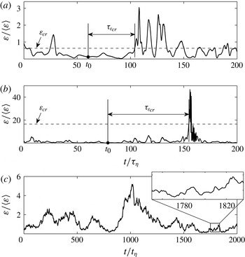
, causing it to break up. Hence it is crucial to control the typical time for which the aggregate experiences a local stress below the critical value, what we call the exit time. In figure 1(a) we show schematically the way in which we propose to estimate the breakup rate, using a real example taken from the evolution of one aggregate. In the figure, we show the time series of kinetic energy dissipation along an aggregate trajectory and the procedure followed to define the exit time. An aggregate released at a time
 $t_{0}$
moves with the flow for a time
 ${\it\tau}_{{\it\varepsilon}_{cr}}$
, after which the local dissipation exceeds for the first time the critical threshold
 ${\it\varepsilon}_{cr}$
(indicated by the dashed line in figure 1
a) where the aggregate breaks up. The first crossing of
 ${\it\varepsilon}_{cr}$
thus defines the exit time,
 ${\it\tau}_{{\it\varepsilon}_{cr}}$
, which is the basic quantity for determining breakup rates.
(a,b) Definition of the exit time
 ${\it\tau}_{{\it\varepsilon}_{cr}}$
(see text) for two typical trajectories in a homogeneous and isotropic flow: (a) time series of energy dissipation along an aggregate trajectory for a low-turbulent-intensity trajectory; (b) the same but in the presence of a strongly turbulent burst; in both panels the dashed line indicates the critical dissipation. (c) A typical evolution of the energy dissipation for an aggregate evolving in a STF; notice the absence of strong fluctuations in this case. In each panel the horizontal axis is normalized by the Kolmogorov time scale
 ${\it\tau}_{{\it\eta}}=({\it\nu}/\langle {\it\varepsilon}\rangle )^{1/2}$
.

To measure the exit time of aggregates, the following protocol is applied (Babler et al.
Reference Babler, Biferale and Lanotte2012). (i) At a time
 $t_{0}$
, a given number of aggregates is released at a random location within a domain
 ${\it\Omega}$
of a stationary flow. (ii) Aggregates released at a point where the local dissipation exceeds
 ${\it\varepsilon}_{cr}$
are ignored, as breakup would have already occurred before the aggregates could reach that point. (iii) Each of the remaining aggregates is followed over time until the local dissipation exceeds the critical dissipation
 ${\it\varepsilon}_{cr}$
; the time lag from release to the breakup defines the exit time
 ${\it\tau}_{{\it\varepsilon}_{cr}}$
for that aggregate. (iv) Fragments formed upon breakup of an aggregate are discarded. The breakup rate for the given threshold and domain of release is then given by the inverse of the mean of the exit time, computed as the ensemble average over many time histories:
 $$\begin{eqnarray}f_{{\it\varepsilon}_{cr}}=\frac{1}{\langle {\it\tau}_{{\it\varepsilon}_{cr}}\rangle }.\end{eqnarray}$$
Equation (2.4) provides a valid definition of the breakup rate that is applicable to both homogeneous and non-homogeneous flows. However, it is important to notice that its implementation requires one to observe the particles for a sufficiently long time in order to confidently estimate the mean exit time. This can be very challenging for measurements made in the field or in a laboratory, and for large values of
 ${\it\varepsilon}_{cr}$
that occur only rarely. Hence, approximations to the breakup rate given by (2.4) are desirable. One such approximation, applicable to homogeneous flows, is obtained by considering the diving time, defined as the time lag between two consecutive crossings of the critical dissipation (Loginov Reference Loginov1985). In homogeneous flows, the diving time can be obtained using the Rice theorem for the mean number of crossings per unit time of a differentiable stochastic process, leading to the following proxy for the breakup rate (Babler et al.
Reference Babler, Biferale and Lanotte2012):
 $$\begin{eqnarray}f_{{\it\varepsilon}_{cr}}^{(E)}=\frac{\displaystyle \int _{0}^{\infty }\dot{{\it\varepsilon}}p_{2}({\it\varepsilon}_{cr},\dot{{\it\varepsilon}})\text{d}\dot{{\it\varepsilon}}}{\displaystyle \int _{0}^{{\it\varepsilon}_{cr}}p({\it\varepsilon})\text{d}{\it\varepsilon}},\end{eqnarray}$$
where
 $p_{2}({\it\varepsilon},\dot{{\it\varepsilon}})$
is the joint probability density function (p.d.f.) of the dissipation and its time derivative,
 $p({\it\varepsilon})$
is the p.d.f. of
 ${\it\varepsilon}$
and the superscript ‘(
 $E$
)’ stands for ‘Eulerian’, indicating that the fragmentation rate is estimated without the need of Lagrangian properties.
Another important and potentially useful approximation can be derived by considering the time evolution of the number of aggregates. In the case where breakup is driven by an uncorrelated force field, the breakup rate can be written as
 $$\begin{eqnarray}f_{{\it\varepsilon}_{cr}}^{(N)}=-\frac{\text{d}\ln N_{{\it\varepsilon}_{cr}}(t)}{\text{d}t},\end{eqnarray}$$
where
 $N_{{\it\varepsilon}_{cr}}(t)$
is the number of aggregates at time
 $t$
after their release. The latter is simply related to the exit-time measurements described above by the relation
 $$\begin{eqnarray}N_{{\it\varepsilon}_{cr}}(t)/N_{{\it\varepsilon}_{cr}}(0)=1-\int _{0}^{t}p_{{\it\varepsilon}_{cr}}({\it\tau})\text{d}{\it\tau},\end{eqnarray}$$
where
 $N_{{\it\varepsilon}_{cr}}(0)$
is the number of aggregates successfully released into the flow and
 $p_{{\it\varepsilon}_{cr}}({\it\tau})$
is the p.d.f. of the exit time for a threshold
 ${\it\varepsilon}_{cr}$
.
2.2. Flow fields
2.2.1. Boundary layer flow (BLF)
We consider a zero-pressure-gradient flow, i.e. the case of a thin flat plate immersed in a uniform steady stream of viscous fluid with undisturbed characteristic velocity
 $U_{0}$
. The no-slip boundary condition is applied on the flat plate. The viscous stresses generated by the flat plate retard the fluid elements close to the wall, so that the fluid zone close to the flat plate has a velocity lower than the free stream value
 $U_{0}$
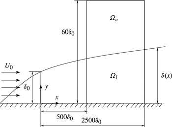
. The resulting flow is known as ‘boundary layer flow’ (BLF). A sketch of the flow configuration is displayed in figure 2. A typical measure of the boundary layer thickness is the so-called geometric thickness,
 ${\it\delta}$
, defined as the distance perpendicular to the wall where the flow reaches 99 % of the undisturbed free stream velocity. It is known from experiments and from simple dimensional arguments that the geometric thickness increases as one moves downstream along the flat plate, implying that the BLF is a spatially evolving flow with a strong inhomogeneity in the wall-normal direction and a weaker evolution in the wall-parallel directions. Different, though somehow equivalent, measures of the characteristic boundary layer thickness exist, such as the displacement thickness
 ${\it\delta}^{\ast }$
and the momentum thickness
 ${\it\theta}$
, which take into account the mass and the momentum loss inside the boundary layer (Schlichting Reference Schlichting1968).
Schematic of the BLF: the two different seeding regions are labelled
 ${\it\Omega}_{i}$
, for aggregates released inside the boundary layer, and
 ${\it\Omega}_{o}$
, for aggregates released outside the boundary layer. Here
 ${\it\delta}(x)$
represents the geometric boundary layer thickness where the mean velocity is 99 % of the free stream velocity
 $U_{0}$
;
 ${\it\delta}_{0}$
denotes the boundary layer thickness in the inlet section of the computational domain;
 $x$
and
 $y$
denote the streamwise and wall-normal coordinates, respectively.

A DNS of the BLF was performed using the pseudospectral Navier–Stokes solver SIMSON (Chevalier et al.
Reference Chevalier, Schlatter, Lundbladh and Henningson2007). The computational domain has a size of
 $(3000{\it\delta}_{0})\times (100{\it\delta}_{0})\times (120{\it\delta}_{0})$
in the streamwise, wall-normal and spanwise directions, where
 ${\it\delta}_{0}$
denotes the geometric boundary layer thickness at the inlet section of the computational domain. The numerical resolution is
 $4096\times 384$
Fourier modes in the wall-parallel plane and 301 Chebishev modes in the wall-normal direction. A localized forcing close to the inlet, random in time and in the spanwise direction, is used to induce the laminar–turbulent transition. The characteristic Reynolds number of the flow, based on the momentum thickness
 ${\it\theta}$
, ranges from
 $Re_{{\it\theta}}=200$
at the inlet to
 $Re_{{\it\theta}}=2500$
at the end of the domain. The resulting turbulent flow is analogous to that described in Sardina et al. (Reference Sardina, Schlatter, Picano, Casciola, Brandt and Henningson2012b
, Reference Sardina, Picano, Schlatter, Brandt and Casciola2014), where the transport and dispersion of inertial particles in boundary layers is studied.
Aggregates are released in two regions: inside the boundary layer (labelled
 ${\it\Omega}_{i}$
in figure 2) and outside the boundary layer (labelled
 ${\it\Omega}_{o}$
in figure 2). The release regions span the streamwise interval from
 $500{\it\delta}_{0}$
to
 $2500{\it\delta}_{0}$
so as to avoid interferences due to the tripping forcing that promotes transition to turbulence. The height of the total release region is
 $60{\it\delta}_{0}$
, and the difference between
 ${\it\Omega}_{i}$
and
 ${\it\Omega}_{o}$
is determined by the local geometric thickness of the boundary layer. The latter ranges from
 $15{\it\delta}_{0}$
at the beginning of the release region to
 $45{\it\delta}_{0}$
at the end of the release region. The release regions were chosen with regard to the spatial distribution of the mean energy dissipation, which, as shown below, shows strong variation in the wall-normal direction while exhibiting only a slow decay in the streamwise direction. A total of
 $2\times 10^{6}$
tracer aggregates are released into the flow. Aggregate trajectories are obtained by integrating the velocity field (2.1). The fluid velocity and its spatial derivatives at the position of the aggregate are quantified by means of a fourth-order spatial interpolation, while a second-order Adams–Bashforth scheme is used for integration of (2.1). Further details about the numerics of the Lagrangian tracking solver can be found in Sardina et al. (Reference Sardina, Schlatter, Brandt, Picano and Casciola2012a
,Reference Sardina, Schlatter, Picano, Casciola, Brandt and Henningson
b
).
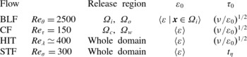
An additional point concerns the characteristic energy dissipation used for normalizing the measured breakup rates. As the BLF is evolving in both the streamwise and wall-normal directions, to define a characteristic dissipation some additional constraints are required, i.e. a specific downstream distance or a spatial domain at which the characteristic dissipation is extracted. Here, we consider the inner release region
 ${\it\Omega}_{i}$
and take the characteristic energy dissipation, denoted by
 ${\it\varepsilon}_{0}$
, as the volume average over this domain;
 ${\it\varepsilon}_{0}$
defined in this way is used for datasets of aggregates released both inside and outside the boundary layer. A summary of the properties of this flow is given in table 1.
Parameters of the numerical experiments: here
 ${\it\varepsilon}_{0}$
and
 ${\it\tau}_{0}$
are the characteristic energy dissipation and time scale used to normalize the data. In the BLF and CF, aggregates are released in two regions. In the BLF, aggregates are released inside the boundary layer, in region
 ${\it\Omega}_{i}=\{500<x/{\it\delta}_{0}<2500,y<{\it\delta}(x)\}$
, and outside the boundary layer, in region
 ${\it\Omega}_{o}=\{500<x/{\it\delta}_{0}<2500,{\it\delta}(x)<y<60{\it\delta}_{0}\}$
, where
 ${\it\delta}(x)$
is the boundary layer thickness and
 ${\it\delta}_{0}$
the boundary layer thickness at the entrance to the computational domain. In the CF, aggregates are released in the centre-plane
 ${\it\Omega}_{c}=\{y/h=0\}$
and in the wall region
 ${\it\Omega}_{w}=\{0.933<|y/h|<1\}$
, where
 $y$
is the wall-normal coordinate and
 $h$
the half-channel height. In HIT and STF, aggregates are released homogeneously.

2.2.2. Channel flow (CF)
The flow domain consists of two infinite flat parallel plates, a distance
 $2h$
apart. The origin of the coordinate system is located at the centre of the channel, and the
 $x$
,
 $y$
and
 $z$
axes represent the streamwise, wall-normal and spanwise directions, respectively. Periodic boundary conditions are imposed on the fluid velocity field in homogeneous directions (
 $x$
and
 $z$
), while no-slip boundary conditions are imposed at the walls. The size of the computational domain is
 $L_{x}\times L_{z}\times L_{y}=4{\rm\pi}h\times 2{\rm\pi}h\times 2h$
. The flow is non-reactive, isothermal and incompressible (low Mach number). The shear Reynolds number is
 $Re_{{\it\tau}}=u_{{\it\tau}}h/{\it\nu}=150$
(Marchioli et al.
Reference Marchioli, Soldati, Kuerten, Arcen, Taniere, Goldensoph, Squires, Cargnelutti and Portela2008), where
 $u_{{\it\tau}}=\sqrt{{\it\tau}_{w}/{\it\rho}}$
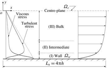
is the shear velocity based on the mean wall shear stress. The flow solver is based on the Fourier–Galerkin method in the streamwise and spanwise directions, and on a Chebishev-collocation method in the wall-normal direction. This solver provides the spatial derivatives required to calculate fluid dissipation along the aggregate trajectory according to (2.3) with spectral accuracy. A Lagrangian tracking code coupled with the flow solver is used to calculate the path of each aggregate in the flow. The aggregate equation of motion (2.1) is solved using a fourth-order Runge–Kutta scheme for time integration. Fluid velocity and velocity derivatives at the aggregate position are obtained using sixth-order Lagrangian polynomials; at the wall, the interpolation scheme switches to one-sided. Further details on the numerical methodology can be found in Marchioli et al. (Reference Marchioli, Soldati, Kuerten, Arcen, Taniere, Goldensoph, Squires, Cargnelutti and Portela2008) and Soldati & Marchioli (Reference Soldati and Marchioli2009). A schematic of the flow is shown in figure 3.
Schematic of the CF: the two different seeding regions are labelled
 ${\it\Omega}_{c}$
for aggregates released in the centre-plane and
 ${\it\Omega}_{w}$
for aggregates released near the wall. On the left side the mean profiles of turbulent and viscous stresses are shown, and on the right side the mean velocity profile is displayed. Here
 $h$
denotes the half-channel height.

Following Pitton et al. (Reference Pitton, Marchioli, Lavezzo, Soldati and Toschi2012), the flow domain is phenomenologically divided into three regions: the wall region, the intermediate region and the bulk region (see figure 3). The wall region comprises a fluid slab with a thickness of 10 wall units. In this region, the viscous stress (representing the mean fluid shear) is maximal while the turbulent stress is close to zero. The intermediate region extends up to 50 wall units from the wall and is characterized by the peak of the fluid Reynolds stresses. The bulk region covers the central part of the channel where all wall stress contributions drop to zero and turbulence is closer to homogeneous and isotropic. Breakup experiments are performed by releasing aggregates in the wall region and at the centre-plane of the bulk region. The two release regions are labelled
 ${\it\Omega}_{w}$
and
 ${\it\Omega}_{c}$
in figure 3. Within each of these release regions,
 $10^{5}$
aggregates are released and their trajectories are tracked and breakup events detected. The characteristic energy dissipation
 ${\it\varepsilon}_{0}$
used to normalize the breakup rate is taken as the volume average over the whole flow domain; see table 1.
2.2.3. Homogeneous turbulence (HIT)
A DNS of three-dimensional incompressible Navier–Stokes turbulence was performed on a triply periodic cubic box, with large-scale statistically homogeneous and isotropic forcing. The external forcing injects energy into the first low-wavenumber shells, by keeping their spectral content constant (Chen et al.
Reference Chen, Doolen, Kraichnan and She1993). The kinematic viscosity is such that the Kolmogorov length scale is comparable to the grid spacing; this choice ensures a good resolution of the small-scale velocity dynamics. The Navier–Stokes equations are solved on a regular grid,
 $2{\rm\pi}$
-periodic, by means of standard pseudospectral methods, with time stepping done using a second-order Adams–Bashforth algorithm. The grid has
 $2048^{3}$
points, and the Taylor scale-based Reynolds number is
 $Re_{{\it\lambda}}\simeq 400$
. Lagrangian particle velocities are obtained by a trilinear interpolation. Details on the numerical integration can be found in Bec et al. (Reference Bec, Biferale, Lanotte, Scagliarini and Toschi2010). The database for this study counts approximately
 $2\times 10^{5}$
tracer trajectories. The characteristic dissipation for normalizing the breakup rate,
 ${\it\varepsilon}_{0}$
, is taken as the mean dissipation over the whole volume; see table 1.
2.2.4. Synthetic flow (STF)
In order to better assess the importance of strong intermittent bursts in the statistics of the energy dissipation felt by the aggregates, it seems useful to study also the dynamical evolution in a STF, whose statistics can be controlled a priori. This flow is constructed to mimic properties of stationary HIT, but with an important and crucial difference: it has Gaussian statistics for the velocity gradients. The STF is realized in a three-dimensional periodic box of size
 $L=2{\rm\pi}$
, with the velocity field written as a Fourier series
 $$\begin{eqnarray}\boldsymbol{u}(\boldsymbol{x},t)=\mathop{\sum }_{\boldsymbol{k}}\hat{\boldsymbol{u}}_{\boldsymbol{k}}^{\prime }(t)\text{e}^{\text{i}\boldsymbol{kx}}.\end{eqnarray}$$
The Fourier coefficients satisfy
 $\hat{\boldsymbol{u}}_{-\boldsymbol{k}}^{\prime }=\hat{\boldsymbol{u}}_{\boldsymbol{k}}^{\prime \ast }$
, where the asterisk indicates the complex conjugate. The summation in (2.8) goes over
 $K=1,\dots ,K_{max}$
shells, each containing
 $N_{K}$
uniformly distributed wavevectors of length
 $|\boldsymbol{k}|=K$
. Incompressibility of
 $\boldsymbol{u}(\boldsymbol{x},t)$
is ensured by taking
 $\hat{\boldsymbol{u}}_{\boldsymbol{k}}^{\prime }$
as the projection of a different vector
 $\hat{\boldsymbol{u}}_{\boldsymbol{k}}$
on a plane perpendicular to
 $\boldsymbol{k}$
. The vector
 $\hat{\boldsymbol{u}}_{\boldsymbol{k}}$
is evolved by a second-order stochastic process originally proposed by Sawford (Reference Sawford1991) to model Lagrangian dispersion. Evolving
 $\hat{\boldsymbol{u}}_{\boldsymbol{k}}$
by a second-order stochastic process results in a velocity field that is differentiable in time, which is a crucial property for measuring temporal statistics such as the exit time. In the second-order process, the spectral acceleration
 $\hat{\boldsymbol{a}}_{\boldsymbol{k}}$
is given by the following stochastic differential equation:
 $$\begin{eqnarray}\text{d}\hat{\boldsymbol{a}}_{\boldsymbol{k}}=-\frac{\hat{\boldsymbol{a}}_{\boldsymbol{k}}}{t_{{\it\eta}}}\text{d}t-\frac{\hat{\boldsymbol{u}}_{\boldsymbol{k}}}{t_{{\it\eta}}t_{L}}\text{d}t+\sqrt{\frac{2{\it\sigma}_{\boldsymbol{k }}^{2}}{t_{{\it\eta}}^{2}t_{L}}}\hspace{2.22198pt}\text{d}\boldsymbol{W},\end{eqnarray}$$
where
 $\text{d}\boldsymbol{W}$
is an incremental Wiener process,
 $t_{{\it\eta}}$
and
 $t_{L}$
are the time scales of acceleration and velocity, respectively, and
 ${\it\sigma}_{\boldsymbol{k}}^{2}$
is the variance of a component of
 $\hat{\boldsymbol{u}}_{\boldsymbol{k}}$
. Due to the isotropy of the flow field,
 ${\it\sigma}_{\boldsymbol{k}}^{2}$
depends only on the modulus of
 $\boldsymbol{k}$
, i.e.
 ${\it\sigma}_{\boldsymbol{k}}^{2}={\it\sigma}_{K}^{2}$
, such that the energy carried by all wavevectors of modulus
 $K$
is
 $E_{K}=(3/2)N_{K}{\it\sigma}_{K}^{2}$
and the total energy is
 $E=(3/2)\langle u^{2}\rangle =\sum _{K=1}^{K_{max}}E_{K}$
. The spectral velocity
 $\hat{\boldsymbol{u}}_{\boldsymbol{k}}$
is simply
 $$\begin{eqnarray}\text{d}\hat{\boldsymbol{u}}_{\boldsymbol{k}}=\hat{\boldsymbol{a}}_{\boldsymbol{k}}\text{d}t.\end{eqnarray}$$
In the present simulations, we set
 $K_{max}=1$
(Bec Reference Bec2005; Zahnow, Maerz & Feudel Reference Zahnow, Maerz and Feudel2011) and take the mean velocity
 $\langle u^{2}\rangle ^{1/2}$
to be small with respect to
 $L/t_{L}$
. For this choice of parameters, the Lagrangian properties are fully determined by the evolution of the spectral coefficients. Following Sawford (Reference Sawford1991), the spectral acceleration decorrelates with
 ${\sim}t_{{\it\eta}}$
while the integral scale of the spectral velocity is equal to
 $t_{L}$
. This allows us to interpret
 $t_{{\it\eta}}$
as the equivalent of the dissipative time scale in turbulence and, furthermore, motivates us to estimate a small-scale Reynolds number for the STF, denoted by
 $Re_{{\it\sigma}}$
, as (Sawford Reference Sawford1991)
 $$\begin{eqnarray}Re_{{\it\sigma}}\sim t_{L}/t_{{\it\eta}}.\end{eqnarray}$$
In this work, we set
 $Re_{{\it\sigma}}=300$
and use
 $t_{{\it\eta}}$
as the characteristic time scale for normalizing the breakup rate; the characteristic dissipation
 ${\it\varepsilon}_{0}$
is taken to be the mean dissipation (table 1). As in the other flows, the aggregate trajectory is obtained by integrating the velocity field, (2.8), while the local dissipation is obtained from (2.3), upon setting the value of the viscosity equal to unity. For measuring breakup rates, several very long trajectories were simulated, from which we then measured diving times. From the diving time, the mean exit time was obtained from an exact relation derived in Babler et al. (Reference Babler, Biferale and Lanotte2012). The breakup rate determined in this way corresponds to the case where aggregates are released homogeneously in the whole domain. The statistical database is as large as
 $1.5\times 10^{6}$
diving events.
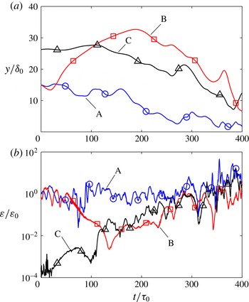
Time series of (a) the wall-normal distance and (b) energy dissipation along typical aggregate trajectories in the BLF. Trajectories A and B correspond to aggregates released in
 ${\it\Omega}_{i}$
, while trajectory C corresponds to an aggregate released in
 ${\it\Omega}_{o}$
(see figure 2). The axes are normalized by
 ${\it\varepsilon}_{0}$
and
 ${\it\tau}_{0}$
given in table 1.

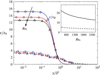
Time-averaged energy dissipation in the BLF as a function of the wall-normal distance at three downstream positions, characterized by
 $Re_{{\it\theta}}=1700$
, 2100 and 2500. Solid lines represent dissipation due to the mean flow, and dashed lines represent dissipation due to velocity fluctuations. The horizontal axis is normalized by the displacement thickness
 ${\it\delta}^{\ast }$
, while the vertical axis is normalized by
 ${\it\varepsilon}_{0}$
given in table 1. The inset shows time-averaged energy dissipation at the wall as a function of
 $Re_{{\it\theta}}$
, representing the streamwise direction; the solid and dashed lines have the same meaning as in the main panel.

Before concluding this section, it is worth stressing the main differences between the STF presented here and a realistic turbulent flow. First, even though we can identify two different time scales in the STF, the dissipation along an aggregate trajectory in STF will not possess any anomalous and intermittent scaling; see e.g. Biferale et al. (Reference Biferale, Boffetta, Celani, Lanotte and Toschi2005). Second, the spatial configuration of the STF is smooth and does not exhibit a Kolmogorov-like
 $-5/3$
spectrum. The former is particularly relevant and will be discussed later in connection with the small efficiency of the STF to break strong aggregates.
3. Results
3.1. Properties of energy dissipation
Energy dissipation plays a decisive role in the breakup of small aggregates. Therefore, in this section we first explore the Lagrangian and Eulerian properties of energy dissipation in the flows under consideration.
Figure 4 shows typical trajectories of tracer-like aggregates in the BLF. Panel (a) shows time series of the wall-normal distance, while panel (b) shows the corresponding local dissipation. For the cases shown in these plots, we assumed that the aggregates are infinitely strong such that they follow the trajectories without breakup (notice that the simple breakup criterion adopted in this work does not allow for determining the size and trajectories of the fragments formed). Among the three trajectories shown, A and B are cases of aggregates released inside the boundary layer, while C is a case of an aggregate released outside the boundary layer. Within the observed time lag, aggregate A is subject to strong fluctuations in dissipation that increase as it moves downstream and as the aggregate comes closer to the wall. On the other hand, aggregate B is first repelled from the boundary layer and moves away from the wall; accordingly, the dissipation decreases and fluctuations are rarer. Later, the aggregate is re-entrained into the boundary layer, which causes dissipation to increase both in magnitude and in the amplitude of fluctuations. The trajectory of aggregate B at this later stage is thus similar to that of aggregate C, which is entrained into the boundary layer after moving downstream for a certain distance.
From these apparently ad hoc examples, it becomes clear that in the presence of a mean flow, breakup events will be controlled by an interplay between the mean flow properties and the relative fluctuations around it. For some aggregate histories the mean profile will control the breakup process, whereas for others breakup is controlled by intense fluctuations of the local energy dissipation around its mean value. As seen below, the balance between the two depends strongly on the geometry of the flow configuration, on the intensity of the turbulent fluctuations and also on where the aggregates are released.
The above discussion can be quantified by looking at the time-averaged profiles of the energy dissipation in the BLF measured at three downstream distances as shown in figure 5, for the mean flow and the fluctuating components. Close to the wall, dissipation assumes large values that are dominated by the mean flow, as shown by the solid curves in figure 5. Dissipation due to turbulent velocity fluctuations (dashed curves) exhibits a flatter profile that expands well beyond the boundary layer thickness
 ${\it\delta}^{\ast }$
. The decrease of dissipation in the streamwise direction is small, as shown in the inset of figure 5, where we plot the time-averaged dissipation at the wall as a function of
 $Re_{{\it\theta}}$
. This explains the relatively constant high magnitude of energy dissipation seen by an aggregate moving within the boundary layer (i.e. trajectory A in figure 4).
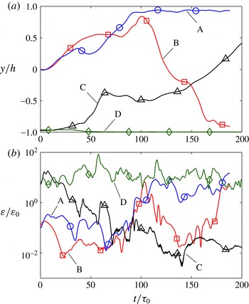
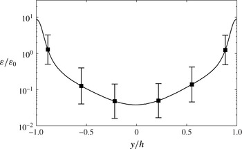
Figures 6 and 7 show analogue data for the CF. Here, aggregates A and B are released in the centre-plane of the channel, while aggregates C and D are released in the wall region. The aggregates released in the centre-plane gradually get entrained by turbulent eddies which transport them to the walls. The entrainment and transport to the wall cause an increase in the magnitude of dissipation seen by the aggregate, while the fluctuations remain persistent. Once they reach the wall, the aggregates have the tendency to stay there for a relatively long time before being re-ejected into the bulk flow. This is seen also for aggregates released close to the wall: aggregate D stays close to the wall while aggregate C is ejected into the bulk flow. From figure 7, where we plot the mean dissipation conditioned on the wall-normal distance, it appears that aggregates are subject to high fluctuations of energy dissipation even when staying in the bulk flow (i.e. away from the walls). Similar to the BLF, dissipation assumes high values close to the walls, while fluctuations in dissipation, indicated by the error bars, are intense throughout the channel.
Time series of (a) the wall-normal distance and (b) energy dissipation along typical aggregate trajectories in the CF. Trajectories A and B correspond to aggregates released in
 ${\it\Omega}_{c}$
, while trajectories C and D correspond to aggregates released in
 ${\it\Omega}_{w}$
(see figure 3). The axes are normalized by
 ${\it\varepsilon}_{0}$
and
 ${\it\tau}_{0}$
given in table 1.

Mean energy dissipation conditioned on the wall-normal distance in the CF. Error bars indicate the root mean square of the conditioned dissipation. The vertical axis is normalized by
 ${\it\varepsilon}_{0}$
given in table 1.

We now consider homogeneous flows. Let us go back to the time series of dissipation along tracer trajectories in HIT shown in figure 1. Panel (a) shows a calm trajectory, i.e. a time interval during which dissipation undergoes moderate fluctuations around the mean. On the other hand, panel (b) shows a trajectory that experiences strong intermittency, i.e. the dissipation undergoes sudden bursts during which its value for a short time exceeds the average dissipation by several standard deviations (Yeung Reference Yeung2001). Such bursts in dissipation are caused by the trapping of particles in intense but short-lived vortex structures (Biferale et al. Reference Biferale, Boffetta, Celani, Lanotte and Toschi2005), which create very high velocity gradients and, as shown below, have a distinct influence on the breakup of strong aggregates.
Panel (c) in figure 1 reports the behaviour of the dissipation along a tracer trajectory in STF. The panel shows the dissipation over a time interval of
 $2000\times t_{{\it\eta}}$
, from which it can be seen that the signal is controlled by two time scales, namely
 $t_{{\it\eta}}$
that controls the fast fluctuations and
 $t_{L}$
that controls the slow fluctuations. Magnifying the time series, as done in the inset of panel (c), highlights the correspondence of the fast fluctuations in the synthetic flow to the fine-scale fluctuations in the homogeneous and isotropic turbulent flow. Also, the time series of dissipation in the synthetic flow describes a much more regular signal than that in turbulence, i.e. intermittent bursts and strong deviations from the mean are absent in this flow. As shown in the next section, this limits the capability of the STF to break strong aggregates.
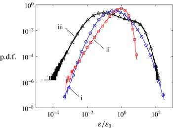
Finally, the Eulerian p.d.f.s of the energy dissipation of the homogenous flows are plotted in figure 8, together with the dissipation p.d.f. of the CF. In agreement with other studies (Vedula, Yeung & Fox Reference Vedula, Yeung and Fox2001; Yeung et al.
Reference Yeung, Pope, Lamorgese and Donzis2006), the dissipation p.d.f. of HIT for the given Reynolds number exhibits a left tail that is close to log-normal and a peak value that is slightly smaller than the mean dissipation. In comparison, the dissipation p.d.f. of the STF is much narrower. Lastly, the dissipation p.d.f. of the CF is very wide as a consequence of the non-homogeneity of the flow. The p.d.f. in fact exhibits two pronounced shoulders, corresponding to the values of
 ${\it\varepsilon}$
in the bulk (left shoulder) and in the wall regions (right shoulder).
Log–log plot of the p.d.f.s of energy dissipation in (i) HIT, (ii) STF and (iii) CF. The vertical axis is normalized by
 ${\it\varepsilon}_{0}$
given in table 1, which for the flows shown corresponds to the volume average.

3.2. Breakup rate measurements
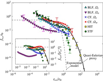
We now have all the ingredients needed to measure and rationalize the breakup rates in turbulent flow upon changing the turbulent intensity and the mean flow configuration. The results are summarized in figure 9, which is the major result of this work. In figure 9 we report the breakup rates measured when one changes the flow configuration, the release region and the method used to estimate
 $f_{{\it\varepsilon}_{cr}}$
. We stress that, to the best of our knowledge, this is the first attempt to perform such a comprehensive examination of a wide range of flow configurations.
Breakup rates plotted against the critical dissipation: exit-time measurements for different flow configurations and release regions (see table 1); the last three points on the right for the HIT data represent estimates from the decay of the number of aggregates according to (2.6). The solid line is a quasi-Eulerian proxy to HIT, given by (2.5); the dashed line is the exponential model (3.1). The inset shows the compensated breakup rates
 $f_{{\it\varepsilon}_{cr}}/[{\it\varepsilon}_{cr}^{-{\it\chi}}]$
with
 ${\it\chi}=0.42$
(Babler et al.
Reference Babler, Biferale and Lanotte2012), where the symbols have the same meaning as in the main panel.

Additionally, we report results from independent predictions, namely the estimate obtained from quasi-Eulerian measurements, given in (2.5), and the approximation based on an exponential fit given in (2.6). As expected, the breakup rate generally decreases with increasing aggregate strength, confirming earlier results suggesting that large aggregates break faster than small ones. Remarkably, except for data from the BLF where aggregates were released outside the boundary layer region (BLF-
 ${\it\Omega}_{o}$
), the breakup rates of the different flows are quite close to each other for small threshold values. We stress that this is not due to a rescaling of the axis but, rather, a consequence of using the characteristic dissipation
 ${\it\varepsilon}_{0}$
and its corresponding time scale for normalizing the axis. The smaller breakup rates for the BLF-
 ${\it\Omega}_{o}$
case reflect the time it takes for the aggregates to be entrained into the boundary layer.
Furthermore, for small
 ${\it\varepsilon}_{cr}$
, the breakup rate shows a power-law-like behaviour that is similar for the different datasets. Power-law breakup rates have been proposed for describing the evolution of the aggregate size distribution in the framework of population balance models, where they lead to adequate agreement with experiments, at least within a certain range of experimental parameters (Babler & Morbidelli Reference Babler and Morbidelli2007). To explore this further, in the inset of figure 9 we show the compensated breakup rate
 $f_{{\it\varepsilon}_{cr}}/[{\it\varepsilon}_{cr}^{-{\it\chi}}]$
using a scaling exponent
 ${\it\chi}=0.42$
. The latter corresponds to a fit of the right tail of the quasi-Eulerian proxy (2.5), which well describes breakup in HIT, as shown by the solid curve in figure 9. A distinct plateau can be observed for aggregates released close to the wall and for aggregates in homogeneous flows; the apparently faster approach to the plateau seen for the wall-bounded flows could be due to a more regular dissipation signal at small
 ${\it\varepsilon}$
for wall-bounded flows as compared to HIT. Deviations from the plateau are only seen for aggregates released in the centre-plane of the channel (CF-
 ${\it\Omega}_{c}$
) and for aggregates released outside the boundary layer (BLF-
 ${\it\Omega}_{o}$
), for which the breakup rate for small
 ${\it\varepsilon}_{cr}$
has a slightly larger scaling exponent. For these release regions, the aggregates first get entrained by turbulent eddies that transport them to the wall. During this entrainment the aggregates gradually experience stronger stress (cf. trajectory A in figure 5). Weak aggregates will therefore, on average, suffer breakup earlier than stronger ones, which causes the breakup rate for these release regions to decrease faster with increasing
 ${\it\varepsilon}_{cr}$
.
For larger threshold values, a levelling off in the decrease of the breakup rate is observed for the wall-bounded flows, i.e.
 $f_{{\it\varepsilon}_{cr}}$
is found to bend upwards as seen in, for instance, the BLF-
 ${\it\Omega}_{o}$
case. This is in contrast to the homogenous flows, for which
 $f_{{\it\varepsilon}_{cr}}$
shows a strong dropoff at large
 ${\it\varepsilon}_{cr}$
(Babler et al.
Reference Babler, Biferale and Lanotte2012). The higher breakup rates for wall-bounded flows are due to the high mean shear close to the wall, which causes aggregates coming close to the wall to rapidly break up. In the homogenous flows, strong aggregates are only broken by the rare excursions of dissipation from the mean caused by intermittency. As these events are rare, the breakup rate exhibits a superexponential dropoff for large dissipation. In the STF, where strong and intermittent excursions from the mean are absent, the dropoff in the breakup rate occurs at much smaller threshold values than in the case of three-dimensional turbulence.
The differences between the STF and real HIT for high threshold values reflects the intriguing dynamics of turbulent fluctuations and the difficulty of modelling them. Indeed, only for these two cases are the statistics of aggregate breakup high enough to allow us to assess the superexponential dropoff and thus reveal the importance of turbulence: extremely robust aggregates break only due to the occurrence of corresponding extremely intense fluctuations, typical of the intermittent nature of small-scale turbulent flows. Any stochastic surrogate that does not possess these critical features would severely underpredict the breakup rate, as is the case for the STF analysed here.
For very large threshold values, a dropoff in the breakup rate is also seen for the CF where the aggregates are released close the wall (CF-
 ${\it\Omega}_{w}$
). It represents the situation where the aggregates are too strong to be broken by the mean shear, and only intense but rare turbulent fluctuations within the near-wall region are able to overcome the aggregate strength. A similar dropoff is likely to occur also for the other cases if trajectories are followed for long enough: recall that the breakup rate represents the inverse of the mean time for which an aggregate survives in the flow. Measuring the small breakup rates expected for large threshold values therefore requires very long trajectories. Exploring this region of high threshold values presents a problem for future work.
In addition, figure 9 shows the breakup rate for the exponential model of Kusters (Reference Kusters1991) (dashed curve). This model is based on the simple dimensional assumption that energy dissipation fluctuations, which govern breakup, have a Gaussian distribution. As a consequence, the following prediction of the breakup rate is obtained:
 $$\begin{eqnarray}f_{{\it\varepsilon}_{cr}}^{(K)}=\frac{(4/15{\rm\pi})^{1/2}}{({\it\nu}/\langle {\it\varepsilon}\rangle )^{1/2}}\exp (-15/2~{\it\varepsilon}_{cr}/\langle {\it\varepsilon}\rangle ).\end{eqnarray}$$
The exponential model predicts a very sharp dropoff at intermediate threshold values and a constant breakup rate for small threshold values, which strongly disagrees with the breakup rate found in the simulations. The discrepancy originates mainly from the simplified assumption of a Gaussian-like dissipation.
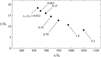
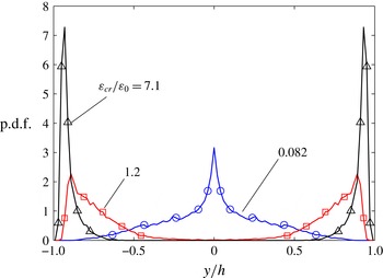
The observation made from figure 9 suggests that weak aggregates in the wall-bounded flows are broken by turbulent fluctuations shortly after their release, while on the other hand strong aggregates survive for a longer time, during which they move further downstream where they eventually suffer breakup due to the mean shear. To explore this further, we examined the spatial location at which breakup occurs in the wall-bounded flows. Two cases are considered: aggregates released inside the boundary layer of the BLF (figure 10) and aggregates released in the centre-plane of the CF (figure 11). Figure 10 shows the average streamwise and wall-normal coordinates at which breakup occurs for different threshold values. As can be seen, with increasing threshold values the aggregates on average move further downstream and come closer to the wall before suffering breakup. The average breakup location for weak aggregates is therefore close to the average location where the aggregates were released. Figure 11 shows the p.d.f. of the breakup location in the CF for three different threshold values. It can be seen that weak aggregates predominantly break in the bulk of the channel close to the point of release, whereas strong aggregates move further downstream and predominantly break close to the wall. This observation is important for applications, and might open a way to tailor turbulent filters with different selection properties depending on the spatially evolving intensity of the turbulent background.
Average
 $(x,y)$
-coordinates of the breakup position for different threshold values of aggregates released in
 ${\it\Omega}_{i}$
in the BLF (see figure 2).

Distribution of the wall-normal distance where breakup occurs in the CF for aggregates released in
 ${\it\Omega}_{c}$
(see figure 3). Different curves correspond to different values of the critical dissipation.

3.3. Evolution of the number of aggregates
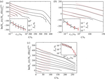
Strong aggregates can move away from the point of release towards the high-shear zones close to the walls: this fact has a clear influence on the breakup behaviour, and leads to the high breakup rates at large threshold values in wall-bounded flows (cf. figure 9). This preferential breakup in specific regions of the flow is also reflected in the time evolution of the number of aggregates,
 $N_{{\it\varepsilon}_{cr}}(t)$
, present in the suspension. From (2.7), it is understood that
 $N_{{\it\varepsilon}_{cr}}(t)$
is proportional to the cumulative exit-time distribution. As in the previous section, we limit the discussion to three cases, namely aggregates released inside the boundary layer in the BLF, aggregates released in the centre-plane in the CF and aggregates released in HIT. Not shown is the time evolution in the STF, for which the time evolution of the number of aggregates has the expected result of a Poisson process.
In figure 12(a), the evolution of the number of aggregates released inside the boundary layer in the BLF is displayed. The figure shows
 $N_{{\it\varepsilon}_{cr}}(t)$
in semilogarithmic coordinates, with the different curves corresponding to different threshold values. It is clear that for small threshold values (lower curves in figure 12
a), the number of aggregates decays exponentially as
 $N_{{\it\varepsilon}_{cr}}(t)\simeq N_{0}\exp (-f_{{\it\varepsilon}_{cr}}^{(N)}\,t)$
. Deviations from the exponential decay observed at later times are due to statistical noise, as the number of aggregates is already very small. The slope
 $f_{{\it\varepsilon}_{cr}}^{(N)}$
, as suggested by (2.6), provides an estimate of the breakup rate. The exponential decay represents the case where the aggregates are broken by uncorrelated turbulent fluctuations in the vicinity of the point of release.
Evolution of the number of aggregates in semilogarithmic coordinates for: (a) BLF with aggregates released in
 ${\it\Omega}_{i}$
; (b) CF with aggregates released in
 ${\it\Omega}_{c}$
; (c) HIT. The curves are plots of
 $\ln (N_{{\it\varepsilon}_{cr}}(t)/N_{{\it\varepsilon}_{cr}}(0))$
for different threshold values normalized by the slope
 $f_{{\it\varepsilon}_{cr}}^{(N)}$
of the pure exponential decay. For clarity, the curves are shifted upwards by a fixed increment such that
 ${\it\varepsilon}_{cr}$
increases from bottom to top. The dashed lines indicate the linear regions used to fit
 $f_{{\it\varepsilon}_{cr}}^{(N)}$
. In each panel, the inset shows the breakup rate as a function of the critical dissipation obtained from exit-time measurements (solid symbols) and from linear fits to
 $\ln N_{{\it\varepsilon}_{cr}}(t)$
(open symbols); the former is the same as the data plotted in figure 9. The solid line in the inset of (c) shows the quasi-Eulerian proxy (2.5).

On the other hand, for large threshold values (upper curves in figure 12
a), the evolution of the number of aggregates shows a different pattern: after an exponential decay at earlier times, a relaxation sets in at intermediate times, which eventually turns into an abrupt decrease at later times. Of these three stages, the relaxation following the exponential decay of
 $N_{{\it\varepsilon}_{cr}}(t)$
is caused by aggregates surviving early breakup and moving away from the point of release. However, later, when these aggregates come close to the wall, they suffer abrupt breakup as represented by the third stage.
The good news here is that despite such non-trivial time evolution, estimating the breakup rate from the linear segments of
 $\ln N_{{\it\varepsilon}_{cr}}(t)$
provides a reasonable approximation. This is shown in the inset of figure 12(a), where we compare the breakup rate measured by the mean exit time, as plotted in figure 9, with the estimation from the linear segments. The latter is very close to the former, which implies that for the threshold values considered, the rate of breakup in the BLF is controlled by the early breakup events in the vicinity of the point of release of the aggregates.
The evolution of the number of aggregates released in the centre-plane of the CF is shown in figure 12(b). As in the BLF, for small threshold values (lower curves in figure 12
b), the number of aggregates decays exponentially, implying that the aggregates are broken by short-time correlated turbulent fluctuations in the vicinity of the point of release. On the other hand, for large threshold values (upper curves in figure 12
b), the evolution of
 $N_{{\it\varepsilon}_{cr}}(t)$
is delayed and its decay sets in only after the aggregates have been in the flow for a certain time. This delay reflects the time it takes for the aggregates to get entrained into turbulent eddies, which transport them to the higher-shear regions close to the wall where they eventually suffer breakup. The breakup rate estimated from fitting the linear segments of
 $\ln N_{{\it\varepsilon}_{cr}}(t)$
is shown in the inset of figure 12(b), together with the exact breakup rate obtained from exit-time measurements as plotted in figure 9. Good agreement with the exact breakup rate is observed also in this case.
Lastly, the evolution of the number of aggregates in HIT is shown in figure 12(c). In contrast to the wall-bounded flows, no qualitative difference in the decay of
 $N_{{\it\varepsilon}_{cr}}(t)$
for different threshold values is seen, and for all threshold values an exponential decay is observed, as indicated by the dashed lines. The breakup rate estimated from this initial decay is shown in the inset of figure 12(c), together with the exact breakup rate from figure 9. The latter is available up to threshold values
 ${\it\varepsilon}_{cr}/\langle {\it\varepsilon}\rangle \sim 5$
; beyond this value, exit times are large compared with the duration of our numerical simulation, which precludes exact measurements of the breakup rate. As can be seen from the inset, for threshold values smaller than
 ${\it\varepsilon}_{cr}/\langle {\it\varepsilon}\rangle \sim 5$
, the approximated breakup rate is very close to the exact breakup rate, while for larger threshold values it is in good agreement with the quasi-Eulerian proxy shown by the solid curve. This close agreement indicates that breakup in HIT resembles breakup in short-time correlated force fields, which justifies modelling breakup as a first-order rate process.
4. Conclusions
We have reported the first systematic study concerning the estimation of the breakup rate of small aggregates in fully developed turbulence upon changing both the flow configuration (bounded and unbounded) and the injection region (relevant only for the bounded-flow cases). Also, we have discussed theoretical and phenomenological ideas concerning the definition of the breakup rate in terms of the so-called exit times measured along the trajectories of all aggregates, or in terms of other proxies, such as breakup rates defined by means of fully Eulerian quantities or by using a fast decorrelation hypothesis along Lagrangian trajectories. Our main approximations are the assumptions that breakup occurs instantaneously once the dissipation at the position of the aggregate exceeds a predefined threshold value and that aggregates behave like tracers with only a one-way coupling with the flow (i.e. no inertia and no feedback on the flow). In future work, the former restriction could be overcome by considering certain time-relaxation properties of the aggregate backbone; the latter can be relaxed by considering inertial aggregates (still one-way coupling).
We have found that breakup is typically the result of two competing effects: a systematic influence of the mean turbulent profile, overlaid by intermittent and bursty events induced by turbulent fluctuations. In turbulent regions dominated by small dissipation events, important for large and easy-to-break aggregates, the breakup rate shows a similar pattern in all flows considered. In particular, we found that the breakup rate in the different flows exhibits a qualitatively similar power-law scaling. This can be explained by noticing that weak aggregates are broken by turbulent fluctuations in the vicinity of the point of release. As the local properties of turbulence at the injection point are expected to be similar, in dimensionless units, the breakup rate assumes similar values.
On the other hand, breakup rates driven by large dissipation events are significantly different between the four flows. Compared to HIT, the bounded flows lead to persistently high breakup rates even for large values of the threshold dissipation. This is due to the fact that in non-homogeneous flows, aggregates can be broken also by the mean flow if they travel enough to reach regions close to the boundary. On the contrary, the STF shows very small breakup rates for large threshold dissipations, due to the absence of both a mean profile and intense intermittent fluctuations characteristic of realistic homogeneous and isotropic turbulent flows.
The study presented here can be viewed as a first step towards the systematic development of models for aggregation kernels and breakup rates, to be used in spatially distributed population balance and compartment models. Furthermore, it helps us to devise experiments for measuring breakup rates. Experimental approaches to measuring breakup rates can be divided into two types. One type of approach measures the time evolution of the aggregate size distribution, from which the breakup rate is deduced, for example by means of a PBE model. The difficulty of this approach is that the time resolution for measuring the size distribution of such small aggregates is of the order of seconds, at best. Also, as the resolution of the measured size distributions is relatively coarse, the PBE model typically needs a predescribed function for the breakup rate. Despite these difficulties, results from this approach have yielded valuable insights into aggregate breakup: it was found that under certain conditions, a power-law breakup rate is in agreement with experimental data (Babler & Morbidelli Reference Babler and Morbidelli2007). A power-law breakup rate in the limit of small threshold dissipation (corresponding to large aggregates) was also found in our study. In the second type of approach, discrete breakup events of aggregates are observed using, for example, stereoscopic microscopy together with particle velocity tracking. Such an approach has been pursued by Lüthi and coworkers (Saha Reference Saha2013). However, the experiments turned out to be fairly tedious in terms of both following the aggregate and observing its breakup. Hence, the methodology of and insight provided by our work can serve as valuable input for the experimentalist.
Acknowledgements
Computer time provided by SNIC (Swedish National Infrastructure for Computing) is gratefully acknowledged. DNS of homogeneous and isotropic turbulence were performed HPC Centre CINECA (Italy). M.U.B. was financially supported by the Swedish Research Council VR (grant no. 2012-6216). L.B. acknowledges partial funding from the European Research Council under the European Community’s Seventh Framework Program, ERC Grant Agreement no. 339032. EU-COST action MP0806 is kindly acknowledged.