Null Hypothesis Significance Testing and p-values

Ronald Aylmer Fisher (Reference Fisher1925) established the foundations of Null Hypothesis Significance Testing (NHST). Subsequently, Neyman and Pearson, (Reference Neyman and Pearson1928a, Reference Neyman and Pearson1928b) proposed a slightly different approach. The point of departure for Fisher's approach was to start from the population and determine the probability that the sample (i.e., the group being studied) had been drawn from a given population. It required only one hypothesis: the null hypothesis (H₀), usually stated as there being no statistically significant difference between two groups on the variable being investigated. Neyman and Pearson's approach (which Fisher vehemently opposed) was to start from the sample and determine the probability that it was from a given population that the sample was drawn. This approach required an alternative, or experimental hypothesis (H₁), usually stated as there being a statistically significant difference between two groups on the variable being investigated, and against which the null hypothesis would be evaluated. Fisher's approach has been regarded as significance testing and that of Neyman and Pearson as null hypothesis testing (Huberty & Pike, Reference Huberty and Pike1999). Over the years, reasoning in statistical inference adopted in behavioural research, and still in current use, is an amalgam of both (Falk & Greenbaum, Reference Falk and Greenbaum1995). Gigerenzer (Reference Gigerenzer, Keren and Lewis1993) attributes the confusion and misconceptions that plague NHST to this hybridisation.

The ‘hybrid logic’ of NHST is usually applied as follows. We might wish to investigate the effectiveness of an intervention aimed to improve the ability of patients with stroke to remember appointments. In order to do so, two randomly drawn samples of patients could be studied: an experimental sample of who received the intervention and a control sample of those who did not. The efficacy of the intervention could then be examined by comparing the mean number of appointments remembered by the treated group ( ${\skew3\overline{X}_{\rm{T}}}$ ) and the control group ( ${\skew3\overline{X}_{\rm{C}}}$ ). The null hypothesis would generally be expressed as H₀: ${\skew3\overline{X}_{\rm{T}}} = {\skew3\overline{X}_{\rm{C}}}$ , and the alternative or experimental hypothesis as H₁: ${\skew3\overline{X}_{\rm{T}}} \ne {\skew3\overline{X}_{\rm{C}}}$ if two-tailed or H₁: ${\skew3\overline{X}_{\rm{T}}} > {\skew3\overline{X}_{\rm{C}}}$ if one-tailed. By convention, the criterion for significance, α, is usually set at 0.05 (it is worth keeping in mind that Fisher chose the 0.05 level without providing any theoretical basis or rationale). An independent samples t-test could be used to analyse the data (note that the same reasoning applies if any other statistical test is used). If the p-value yielded by the t-test was <0.05, a common belief is that there would be less than a 5% chance of H₀ being true and would confidently reject it. We have proven that the treatment was effective. Seen from this perspective, NHST provides neat and unambiguous answers, hence its seductiveness. But closer scrutiny shows that our understanding of the process and interpretation of the results of statistical tests is, probably, rather muddled.

Berkson (Reference Berkson1938) was one of the first to discuss the shortcomings of the NHST, and there has been lively debate ever since (e.g., Carver, Reference Carver1978; Clark, Reference Clark1963; Cohen, Reference Cohen1990; Glaser, Reference Glaser1999; Gliner, Leech & Morgan, Reference Gliner, Leech and Morgan2002; Meehl, Reference Meehl1967; Nickerson, Reference Nickerson2000; Rozeboom, Reference Rozeboom1960). Coming to grips with NHST requires a clear understanding of the relation between populations and samples, the difference between the sampling distribution and the population distribution, the postulates of the law of large numbers and the central limit theorem. It also requires a clear understanding of the meaning of significance level, H₀, H₁ and p-values, as well as the interrelationship between them (Castro Sotos, Vanhoof, Van den Noortgate & Onghena, Reference Castro Sotos, Vanhoof, Van den Noortgate and Onghena2007). However, misconceptions about NHST abound (Krishnan & Idris, Reference Krishnan and Idris2014; Lambdin, Reference Lambdin2012; Vallecillos & Batanero, Reference Vallecillos and Batanero1997a, Reference Vallecillos and Batanero1997b; Vallecillos, Reference Vallecillos2001).

An overarching problem with NHST is that it does not do what we want it to do (Cohen, Reference Cohen1990: Cohen, Reference Cohen1994; Falk & Greebaum, Reference Falk and Greenbaum1995; Kirk, Reference Kirk1996). What the researcher wants to know is the probability of H₀ being true given the observed data D; this can be expressed as P(H₀|D). What NHST gives us is the probability of obtaining the observed data if H₀ is true, which can be expressed as P(D|H₀). Clearly, P(H₀|D) is not the same as P(D|H₀). If the statistical test employed yields significant results (i.e., p ≤ 0.05) all it tells us is that P(D|H₀) is low. This does not necessarily mean that P(H₀|D) is also low and consequently it is erroneous to conclude that a significant result means that H₀ is false. Carver (Reference Carver1978) provided a very clear illustration of this. He suggested that the probability of a person being dead (symbolised as D), if they had been hanged (symbolised as H) can be expressed as P(D|H). According to Carver, this probability would be very high. The reverse, the probability that a person has been hanged, given that the person is dead can be expressed as P(H|D). However, it is abundantly clear that P(H|D) is likely to be very small. Carver points out that in his example it is unlikely that anyone would mistakenly substitute P(D|H) for P(H|D). By analogy, this is what occurs in NHST.

What Should Be Done?

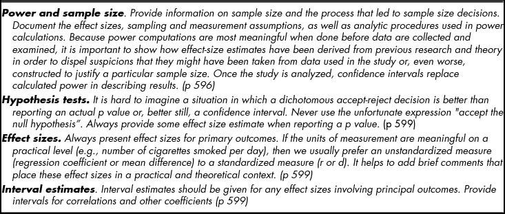
In 1994, Cohen published a seminal article reviewing the problems and misunderstandings that had beleaguered NHST over the previous four decades. Following the article's publication, the Board of Scientific Affairs of the American Psychological Association (APA) appointed the Taskforce on Statistical Inference (APA-TSI) to consider the role of NHST in psychological research and make recommendations regarding analysis of quantitative research in psychology (Wilkinson et al., Reference Wilkinson1999). There had been expectations in some quarters that there would be an outright ban on NHST (Kirk, Reference Kirk1996). This did not occur and the Taskforce made several recommendations that researchers should implement in conjunction with NHST and reporting of p-values. These are summarised in Table 1.

TABLE 1

Recommendations of the Taskforce on Statistical Inference APA Board of Scientific Affairs Recommendations (Adapted from Wilkinson et al., Reference Wilkinson1999)

In a nutshell, the main focus of the Taskforce recommendations was that results of NHST should report exact p-values and not just dichotomous decisions such as accept/reject H₀. More importantly, it was recommended that in addition to p-values, effect size (ES) should also be reported, as well as the precision or confidence interval (CI) of the ES. These recommendations were incorporated in subsequent editions of the APA Publication Manual. Prior to the 6th edition of the Publication Manual, the Working Group on Journal Article Reporting Standards (JARS) formulated precise reporting standards for manuscripts submitted to APA journals, including reports of experimental evaluations of interventions and reports of meta-analyses (APA Publications and Communications Board Working Group on Journal Article Reporting Standards, 2008). The recommendations require that the statistical methods used to analyse data must be clearly described and justified. If inferential statistics are used, the a priori Type I error rate adopted must be reported. Differences between intended and actual sample size, power analysis (or methods used to determine precision of parameter estimates) should also be reported. It is not mandated that statistical significance levels (i.e., p-values) need to be reported, but findings must include ESs and CIs.

Prior to the publication of the 1999 APA-TSI recommendations, ESs were not frequently reported. In a survey of 391 articles that used inferential statistics published in four major psychology journals (three of which were APA journals), Kirk (Reference Kirk1996) found that while just over 6% of articles reported three or more measures of ES, between 23% and 88% in the various journals did not report any such measure. Keselman et al. (Reference Keselman, Huberty, Lix, Olejnik, Cribbie, Donahue and Levin1998) reviewed all articles using analysis of variance designs published in the 1994–1995 issues of 17 prominent education and psychology research journals. Only 41 (10%) of the 411 analyses examined reported ESs.

In a comprehensive review of 32 studies investigating ES reporting practices in psychology, education, behavioural research and rehabilitation journals, Peng, Chen, Chiang and Chiang (Reference Peng, Chen, Chiang and Chiang2013) found that since the publication of the 1999 APA-TSI recommendations reporting rate of ESs and, to a lesser extent, CIs had improved. Nonetheless, rate of reporting for ESs was still generally less than 50%, and even lower for CIs. A similar pattern was evident in the neuropsychological literature. In a survey of 406 articles published in The Archives of Clinical Neuropsychology between 1990 and 2004, Schatz, Jay, McComb and McLaughlin (Reference Schatz, Jay, McComb and McLaughlin2005) found that there was a significant increase in ES reporting after the release of the APA-TSI recommendations. Prior to the APA-TSI report (1990–1992) 4.3% of articles reported ESs. In the period commensurate with and shortly after the APA-TSI report (1996–2000), 22.4% reported ES, and in the subsequent period (2001–2004) ES was reported in 29.4% of articles.

Effect Size

A significant p-value indicates the likelihood of obtaining the observed data if H₀ is true. The magnitude of p (e.g., <0.05 vs. <0.0001) does not reflect the size (or the importance) of the intervention effect (Gliner, Leech, & Morgan, Reference Gliner, Leech and Morgan2002). Smaller p-values (e.g., <0.0001) are, however, often and erroneously interpreted to mean that the intervention effect is larger. Cohen (Reference Cohen1990) points out that ‘Because science is inevitably about magnitudes, it is not surprising how frequently p values are treated as surrogates for effect sizes’. (p. 1309). Glasser (Reference Glaser1999) illustrates one aspect of this fallacy by considering a hypothetical Randomised Control Trial to investigate a dietary intervention for lowering cholesterol. The intervention reduces cholesterol levels from 243 to 238 mg/100 ml in the experimental group but there is no change in the control group. Glasser suggests that most clinicians might not consider changing clinical practice on the basis of such trivial effect (only 5 mg/100 ml), but would probably attribute more importance to the study findings if p was <0.05.

Cohen is credited with introducing the concept of ES to psychological research and measures of ES have been available for at least 60 years (Huberty, Reference Huberty2002). In essence, an ES provides measure of the degree to which the observed data differ from the expectations postulated in H₀ (Cohen, Reference Cohen1994). An ES quantifies the size of a difference between two groups and provides point estimate of treatment effect, that is, how well an intervention works. ESs are independent of sample size, whereas p-values reflect both ES and sample size. ESs are an important tool in reporting and interpreting treatment effectiveness. ESs can be calculated using either ‘raw’ differences between, say, the means of the treatment and control group (absolute ES), or as standardised differences. The problem with ‘raw’ ESs is that if the scale used to measure the outcome variable is not readily interpretable (e.g., rating on anxiety on a 0–10 scale) the meaning of the ES magnitude is unclear. Moreover, the magnitude of ‘raw’ ESs is influenced by the scale used to measure the outcome variable which further complicates interpretation. Standardised ESs take into account group variability are ‘metric free’ and are analogous to z-scores. Moreover, because they are ‘metric free’ the results of different studies addressing the same issue but using different outcome measures can be directly compared, making it possible to conduct meta-analyses.

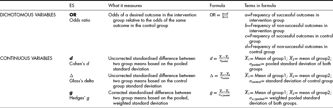
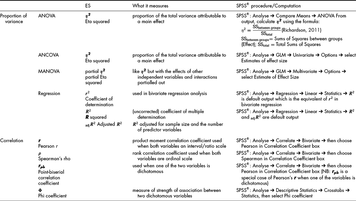
ESs can be classified into two main ‘families’: the d-family for measures of between-group differences and the r-family, for measures of association (Ellis, Reference Ellis2010). A selection of common ESs in each family is shown in Tables 2 and 3.

TABLE 2

d Family Effect Sizes – Measures of between Group Differences

TABLE 3

r Family Effect Sizes – Measures of Association

As Cohen (Reference Cohen1988) points out, hypotheses about differences between two means are the most frequently tested in behavioural research. Consequently, Cohen's d (Cohen, Reference Cohen1988) is a common used ES in these circumstances, which is fortunate because it, along with Glass's ∆ (Glass, McGaw, & Smith, Reference Glass, McGaw and Smith1981) and Hedges’ g (Hedges, Reference Hedges1981), is easy to calculate. An example, using hypothetical data, of how to calculate each of these ESs is shown in Box 1. Each of these three ES measures expresses the impact of the intervention in terms of standard deviations. The magnitude of the ESs for the hypothetical data calculated by the three different methods is very similar. This is not surprising, given that the numerator in each formula is the same and only slightly different values for the standard deviation (σ) are used in the denominator of each formula.

Box 1:

Consider a study to investigate the effect of a brief memory training intervention on the ability of persons with stroke to recall stories. The hypothetical result for the two groups after the intervention is given below.

• 

Cohen's d (Cohen, Reference Cohen1988): If the standard deviation of the two groups are equal (i.e., σ_C = σ_I ) then either can be used to calculate d , using the formula:

$$\begin{equation*} d = \frac{{{{\skew3\overline{X}}_I} - {{\skew3\overline{X}}_C}}}{\sigma } \end{equation*}$$

If σ_C ≠σ_I , as is the case for the hypothetical data, Cohen suggests that the pooled standard deviation (σ _pooled) is calculated using the formula:

$$\begin{equation*} {\sigma _{{\rm{pooled}}}} = \sqrt {\frac{{\sigma _C^2 + \sigma _I^2}}{2}} \end{equation*}$$

and σ_pooled is then used instead of σ in the formula above.

For the hypothetical data: ${\sigma _{{\rm{pooled}}}} = \sqrt {\frac{{{{4.2}^2} + {{3.4}^2}}}{2}} = \sqrt {\frac{{17.6 + 11.6}}{2}} = \sqrt {\frac{{29.2}}{2}} = \sqrt {14.6} = 3.8$

Calculating d for the hypothetical: $\bm{d} = \frac{{{{\bm{\skew3\overline{X}}}_{\bm I}} - {{\bm{\skew3\overline{X}}}_{\bm C}}}}{{{\bm{\sigma }_{{\rm{pooled}}}}}} = \frac{{17.6 - 15.2}}{{3.8}} = \frac{{2.4}}{{3.8}} = .63\vspace*{6pt}$

Glass'delta (Glass et al., Reference Glass, McGaw and Smith1981): Which group mean (i.e., ${\skew3\overline{X}_I}$ or ${\skew3\overline{X}_C}$ ) is substituted for ${\skew3\overline{X}_1}$ and ${\skew3\overline{X}_2}$ in Glass’ formula is decided by the same considerations outlined above.

Calculating of Δ for the hypothetical: $\Delta = \frac{{{{\bm{\skew3\overline{X}}}_1} - {{\bm{\skew3\overline{X}}}_2}}}{{{\bm{\sigma }_{{\rm{control}}}}}} = \frac{{17.6 - 15.2}}{{4.2}} = \frac{{2.4}}{{4.2}} = .57\vspace*{6pt}$

Hedges’ g (Hedges, Reference Hedges1981): To calculate this ES, the weighted, pooled standard deviation needs to be calculated first. This can be done using the formula:

$$\begin{equation*} {\sigma _{w/{\rm{pooled}}}} = \sqrt {\frac{{\sigma _1^2\left( {{N_1} - 1} \right) + \sigma _2^2\left( {{N_2} - 1} \right)}}{{{N_1} + {N_2} - 2}}} \end{equation*}$$

For the hypothetical data: $\begin{array}{@{}l@{}} = \sqrt {\frac{{\sigma _I^2( {{N_I} - 1} ) + \sigma _C^2( {{N_C} - 1} )}}{{{N_I} + {N_C} - 2}}} = \sqrt {\frac{{{{3.4}^2}( {25 - 1} ) + {{4.2}^2}( {23 - 1} )}}{{25 + 23 - 2}}} = \sqrt {\frac{{277.44 + 388.08}}{{46}}} \\[9pt] \quad \quad \; = \sqrt {\frac{{665.52}}{{46}}} = \sqrt {14.5} = 3.80 \end{array}$

Calculating g for the hypothetical data: $\bm{g} = \frac{{{{\bm{\skew3\overline{X}}}_1} - {{\bm{\skew3\overline{X}}}_2}}}{{{\bm{\sigma }_{{\bm{w}}/{\rm{pooled}}}}}} = \frac{{{{\skew3\overline{X}}_I} - {{\skew3\overline{X}}_C}}}{{{\sigma _{w/{\rm{pooled}}}}}} = \frac{{17.6 - 15.2}}{{3.8}} = \frac{{4.8}}{{3.8}} = .63$

So, which of the ESs should be calculated? If σ for the intervention and control groups are exactly equal, then Cohen's d can be calculated and either σ can be used; this, however, is an unlikely scenario in the real world. If σ for the two groups are reasonably equal, then it can be assumed that they are estimates of the population from which the two groups have been drawn (Ellis, Reference Ellis2010). In this instance, it would be also be appropriate to pool the standard deviations using the formula shown in Box 1 and calculate Cohen's d . The question is: how ‘reasonably equal’ must the standard deviations of the two groups be? Unfortunately, there is no precise criterion for determining this, and researchers must exercise their own judgement. If in doubt, or if the standard deviations of the two are clearly unequal, then the homogeneity of variance assumption is violated and pooling the standard deviations is not appropriate. One solution is to calculate Glass's delta, using the control group σ. The assumption behind this is that the control group σ will not have been influenced by the intervention and will therefore reflect the population σ more faithfully (Ellis, Reference Ellis2010). The robustness of this assumption increases as the size of the control group increases. If the size of the intervention and control groups differs (particularly if the difference is substantial), it is more appropriate to calculate Hedge's g because it uses the weighted pooled σ for the two groups which takes into account group size. Moreover, it might, arguably, be more appropriate in ‘real life’ situations where sample sizes and/or σ for each sample might not always be equal. Turner and Bernard (Reference Turner and Bernard2006) recommend its use because Hedge's g also corrects for the small-sample bias in Cohen's d and converges to it in large samples.

Other ESs listed in Tables 2 and 3 are measures of intervention effect applicable when data analysis involves more than comparison of two means (although a two group, one-way ANOVA data is essentially the same as a t-test). The computation for η ² (top of Table 3) is straight forward from Sums of Squares in the SPSS® output. The formula shown in Table 3 is suitable for main effects in fixed factor designs, but can also be used for univariate contrasts by substituting the SS_{between groups} in the numerator for SS_contrast (Olenik & Algina, Reference Olejnik and Algina2000). Indeed, these authors elaborate the application of η ² to ANCOVA as well as multifactorial, random factors, and mixed designs.

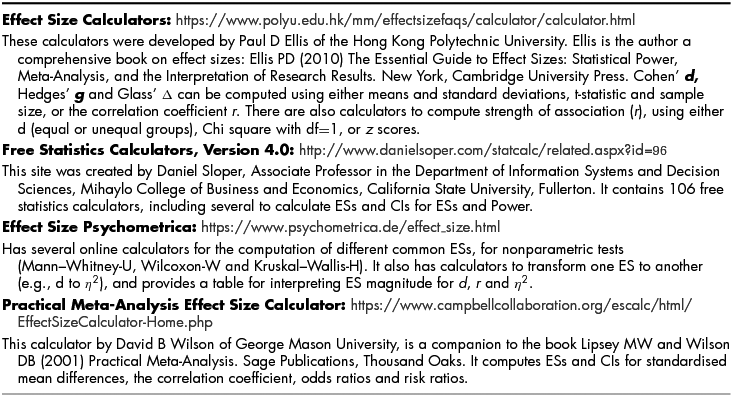
Fortunately, the other ES indices in Table 3 can be directly obtained from SPSS® output. But this is not always the case. Statistical packages commonly used in psychological research, such as SPSS® and SAS®, can calculate other ESs, but this often requires specific syntax that is not available from the drop-down menus. Meyer, McGrath and Rosenthal (Reference Meyer, McGrath and Rosenthal2003) provide syntax patches for calculating Pearson's r and Cohen's d in SPSS® and SAS®, as well as syntax for converting one type of ES to another. Torchiano (Reference Torciano2017) has recently published a package of R-code to calculate various ESs. A more convenient way to calculate ESs, however, is to browse the free on-line calculators listed in Table 5. These sites offer calculators to compute ESs, CIs for ESs, transform one ES to another, as well as many other useful statistical tools. Peng, Chen, Chiang and Chiang (Reference Peng, Chen, Chiang and Chiang2013) have compiled a list of internet resources (Table 5, pp. 203–204) for calculating ESs.

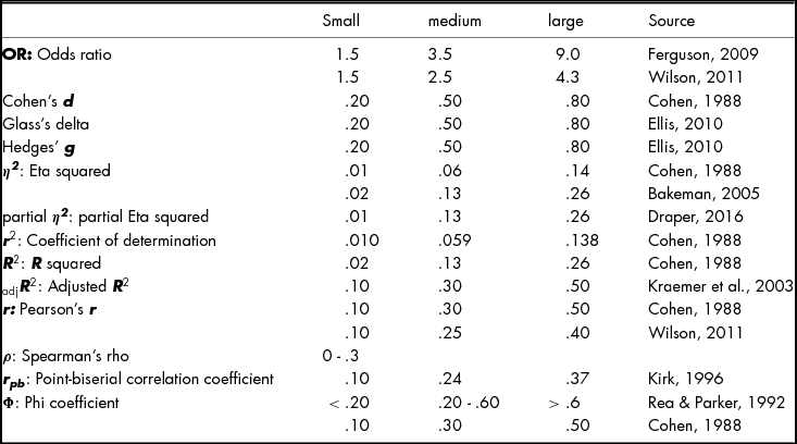
Cohen's ‘rules of thumb’ for interpreting the magnitude of most common ESs have been universally adopted (Table 4) for other ESs. According to Cohen (Reference Cohen1962), a medium ES is visible to the naked eye. He acknowledged that the magnitude of what he labelled small, medium and large ESs was chosen arbitrarily and cautioned the reader to exercise their own judgement. Opinion differs on how to interpret magnitude of other ESs. For example, Kraemer et al. (Reference Kraemer, Morgan, Leech, Gliner, Vaske and Harmon2003) classify the magnitude of d-family ESs as: much larger than typical >1.0, large of larger than typical = .80, medium or typical = .50 and small or smaller than typical = .20. Similarly, they classify the magnitude of r-family effects as: much larger than typical >.70, large or larger than typical = .50, medium or typical = .30 and small or smaller than typical =.10.

TABLE 4

Interpretation of Effect Size

Confidence Intervals

The CI of the ES provides the precision of the estimation. CIs are, in essence, error terms that provides the likely range of the intervention effect (Fethney, Reference Fethney2010; Turner & Bernard, Reference Turner and Bernard2006). As power increases with larger sample sizes the CI range diminishes, indicating greater ES precision (Halsey, Curran-Everett, Vowler, & Drummond, 2015). Estimating CIs for some ESs can be relatively straight forward. Berben, Sereika and Engberg (Reference Berben, Sereika and Engberg2012) describe a simple method for calculating the 95% CI for Cohen's d . The method is illustrated in Box 2, using the hypothetical data from Box 1. In this instance, ES = .63 and the 95% CI = .04–1.22. What this CI tells is that true ES in the population from which the two hypothetical groups (i.e., N_I and N_C ) were drawn is 95% certain to be in the range of .04–1.22. Because the CI does not include zero, we can reasonably assume that there is a positive intervention effect. If the CI had included zero, it would raise the possibility that the observed ES might have been obtained by chance.

Box 2:

Calculation of Confidence Interval for Cohen's d

The first step is to calculate the standard deviation of d using the formula:

• ${\sigma _d} = \sqrt {\frac{{{N_I} + {N_C}}}{{{N_I} \times {N_C}}} + \frac{{{d^2}}}{{( {2/{N_I} + {N_C}} )}}} $ (Cooper, Hedges, & Valentine, Reference Cooper, Hedges and Valentine2009)

Using the hypothetical data from Box 1: N_I = 25, N_C = 23 and d =.63

$$\begin{equation*} \begin{array}{@{}l@{}} {\sigma _d} = \sqrt {\frac{{25 + 23}}{{25 \times 23}} + \frac{{{{.63}^2}}}{{\left( {2/25 + 23} \right)}}} \\ = \sqrt {\frac{{48}}{{575}} + \frac{{.3969}}{{ {48}}}} \\ = \sqrt {0.083 + 0.008} = 0.30 \end{array} \end{equation*}$$

The 95% CI is calculated using the formula:

• 95% CI = d ± (z _0.05/2 × σ _d ) where z _0.05/2 is the z-score for a two-tailed probability of 0.05, which is 1.96. Hence:

• $\begin{array}{@{}l@{}} 95\% \ {\rm{CI}} = .63 \pm ( {1.96 \times 0.30} )\\ \ \quad \quad\quad = .63 \pm ( {0.59} ) \end{array}$

Which means that d ranges between 0.04 and 1.22

Although formulae for calculating CI are available (e.g., Cumming & Finch, Reference Cumming and Finch2001; Li-Ting & Chao-Ying, Reference Li-Ting and Chao-Ying2013), they either require computer intensive iteration procedures or the hand calculations are cumbersome. However, one ‘complication’ with the calculation of ES CIs is that non-central t-distributions (i.e., an asymmetrical distribution not distributed around zero) are used (Howell, Reference Howell2010). Smithson (Reference Smithson2001) provides SPSS® syntax to estimate non-central CIs for various ESs. Fortunately, however, most of the on-line calculators listed in Table 5 also compute CIs.

TABLE 5

Free On-line Calculators

Closing Remarks

NHST does not do what we think it does and the way it works is often misunderstood, but it is too entrenched to disappear completely any time soon. For almost 20 years, there have been clear directives that researches should not rely solely on NHST and report only p-values. A statistically significant result (i.e., p < 0.05) allows the researcher to decide with some degree of confidence that observed differences between groups, namely the ES, are reliable if H₀ were true. This is particularly useful if sample sizes are small. However, a result can be statistically significant merely because the sample size is large, even if the ES is trivial. Moreover, statistical significance is not equivalent to clinical significance, that is whether or not an intervention produces a change that is important and useful in the real world (see for example, Fethney, Reference Fethney2010; Sainani, Reference Sainani2012; Thompson, Reference Thompson2002). On the other hand, even small ESs might be clinically significant. Prentice and Miller (Reference Prentice and Miller1992) suggest that a small ESs might be important when either a small change in the independent variable (for our purposes, the intervention) produces a change in the dependent variable (for our purposes, the target behaviour or primary outcome measure), or when a change is elicited on a dependent variable that is resistant to change.

P-values give us useful information about the probability that the obtained data pertains to samples drawn from the same or different populations. What we want to know in neurorehabilitation is whether or not an intervention has had a ‘real’ or clinically significant effect: measures of ES and their CIs can give us that information.

Financial Support

This research received no specific grant from any funding agency, commercial or not-for-profit sectors.

Conflict of Interest

None.

Ethical Standards

The research does not involve human experimentation.