1 Introduction
Incompressible viscous flow past two-dimensional (2-D) bluff bodies involves complex physics such as the well-known von-Kármán street phenomenon as well as three-dimensional (3-D) wake dynamics as the Reynolds number (
 $Re$
) is increased (Roshko Reference Roshko1954; Williamson Reference Williamson1996a
,Reference Williamson
b
). Due to the two-dimensionality of circular cylinders, some authors have used the 2-D Navier–Stokes equations on multiple planes located along the span of the cylinder as a simplified model of the three-dimensionality without increased computational cost (a.k.a. strip theory method). Such strip theory methods are used in offshore and civil engineering applications to model flow along slender structures where the computational cost of fully resolved simulations is prohibitive, such as marine risers, tow and mooring cable systems and tall pillars. However, the physics inherent in 2-D simulations lead to poor 3-D predictions (Bao et al.
Reference Bao, Palacios, Graham and Sherwin2016), and a better understanding of the evolution from 3-D to 2-D turbulent wakes is needed to improve strip theory methods.
The fluid mechanics of turbulent flows behave quite differently when the spanwise spatial dimension is much more constrained than the others. Instead of having a direct cascade of the turbulence kinetic energy (TKE) from the integral scales down to the dissipative scales, there is a dual cascade of (direct) enstrophy and (inverse) energy. This was first suggested by Kraichnan (Reference Kraichnan1967) and further developed by Leith (Reference Leith1968) and Batchelor (Reference Batchelor1969) (known as the KLB 2-D turbulence theory). More recently, the dual cascade has been demonstrated both experimentally and computationally (for a comprehensive review see Boffetta & Ecke Reference Boffetta and Ecke2012). Studies such as Xiao et al. (Reference Xiao, Wan, Chen and Eyink2009) have shown that physical processes such as vortex thinning and vortex merging dominate the dynamics of 2-D turbulence, generating larger and more intense vortical structures the energy of which piles up at the integral scale for bounded domains.
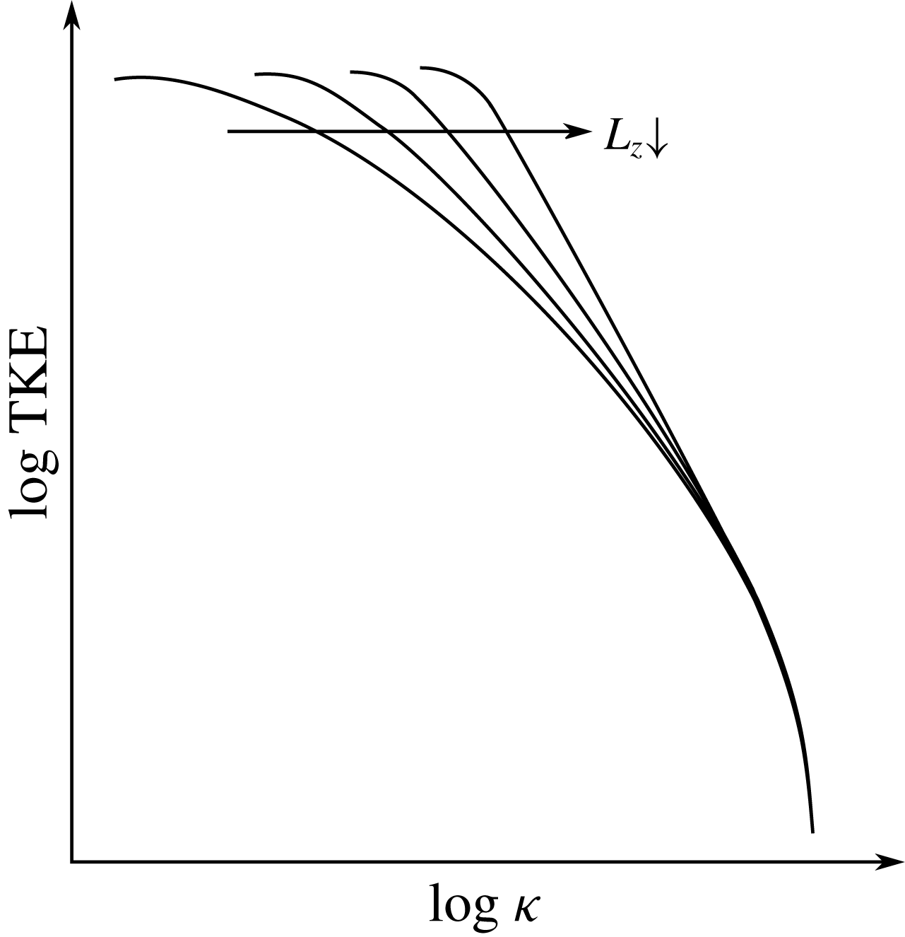
Previous work has studied the transition between 2-D and 3-D dynamics in obstacle-free turbulent flows in detail. The effect of length scale
 $L_{z}$
constriction on the TKE distribution across the scales (or wavenumbers
 $\unicode[STIX]{x1D705}$
) is sketched in figure 1. By constricting the domain, the size of the 3-D energy-containing structures (integral scale structures) is reduced. Since the energy-containing structures feed the inertial subrange structures down to the 3-D small-scale dissipative structures, smaller integral scale structures result in less energy fed into the inertial subrange structures and, consequently, to the dissipative structures. In the 2-D limit, no 3-D dissipative structures are present and, because of the lack of a dissipation mechanism, the turbulent vortical structures can only merge. This creates larger structures promoting an inverse energy cascade as shown in Kraichnan (Reference Kraichnan1967), Leith (Reference Leith1968) and Batchelor (Reference Batchelor1969).
Smith, Chasnov & Waleffe (Reference Smith, Chasnov and Waleffe1996) reviewed the aspect ratio depth effect together with a rotation effect of forced turbulence on a
 $L_{x}\times L_{y}\times L_{z}$
periodic box. It was found that the turbulence dimensionality of the flow depended not only on the geometry constriction (
 $A\equiv L_{z}/L_{x}$
), but also on the rotation intensity
 $\unicode[STIX]{x1D6FA}$
. A critical ratio between the span and the turbulence forcing scale was revealed below which two-dimensionalisation occurred for non-rotating cases. Furthermore, it was found that higher rotation rates induced a more significant 2-D turbulence behaviour and that direct and inverse energy cascades for small and large scales can coexist respectively. Celani, Musacchio & Vincenzi (Reference Celani, Musacchio and Vincenzi2010) found a similar splitting of the turbulence cascade for a critical value of the relative forcing on a depth-restricted periodic box.
Sketch of the TKE cascade distribution across the scales as the span is reduced. By constricting the domain, the integral scale is reduced and the energy-containing scales can feed less energy to the inertial and dissipative scales.

These differences between 2-D and 3-D turbulence dynamics have a significant practical impact. For example, the forces induced on a cylinder are larger in magnitude and variability in 2-D systems (Mittal & Balachandar Reference Mittal and Balachandar1995; Norberg Reference Norberg2003). In an attempt to dissipate the energised vortical structures and to prevent the vortex-merging dynamics of 2-D turbulence, models based on the turbulent-viscosity hypothesis (a.k.a. the Boussinesq hypothesis) are incorporated into 2-D strip theory methods. However, these models assume that the anisotropic Reynolds stress tensor is proportional to the mean rate-of-strain tensor by the scalar turbulent viscosity, which has been proven inaccurate even for simple shear flows (Pope Reference Pope2000, p. 94). A further complication for strip theory is that the presence of walls adds a production mechanism of 3-D turbulence which is able to generate very fine 3-D vortical structures even in highly anisotropic geometries.
A ‘thick’ strip theory method proposed by Bao et al. (Reference Bao, Palacios, Graham and Sherwin2016) showed how strips with a certain thickness are able develop to 3-D turbulence when its span is larger than the wavelength of the Mode B instability of circular cylinders (approximately one diameter). In fact, this instability creates rib-like streamwise vortical structures along the main Kármán 2-D vortices (Noack Reference Noack1999). Therefore, it can be argued that the two-dimensionalisation of the wake arises from the geometry constriction which prevents the rib-like vortices developing when there is not room enough for its natural wavelength. However, the connection between wake and wall turbulence and the persistence of 3-D turbulent structures in constricted span flows has not been fully explored.
This work studies the geometry constriction effect on the turbulence nature of a flow past a circular cylinder at
 $Re=10\,000$
. To do this, a series of simulations ranging from
 $L_{z}=10$
to pure 2-D planes have been considered. As discussed above, the inclusion of a body boundary provides an important change to the turbulence production mechanisms compared to previous research and novel information on the transition and cross-over between 3-D and 2-D turbulence for very constricted domains in wall-generated turbulent shear flows. Multiple turbulence statistics are presented for the wide range constricted wakes, providing new data on the transition from 3-D to 2-D turbulence.
With this intention, we have structured the current paper as follows: § 2 describes the governing equations and the numerical methods as well as the computational details of the simulations. In § 3, the turbulence nature of the wake for the different cases is analysed (similarly to Biancofiore (Reference Biancofiore2014)) and discussed with results such as wake visualisation, velocity temporal spectra at different locations, Lumley’s triangle, TKE spatial plots and vortex-stretching analysis.
2 Problem formulation
This study considers the flow past a circular cylinder with diameter
 $D$
aligned on the
 $z$
direction in a 3-D
 $(35\times 20\times L_{z})D$
rectangular domain, where
 $L_{z}$
is the non-dimensional span. To study the span effect on the turbulence nature of the wake, the following cases have been considered:
 $L_{z}=10,\unicode[STIX]{x03C0},1,0.5,0.25,0.1$
as well as a fully 2-D case.
A Reynolds number of
 $Re=10\,000$
is selected. We define the Reynolds number as,
 $$\begin{eqnarray}Re=\frac{UD}{\unicode[STIX]{x1D708}},\end{eqnarray}$$
where
 $U$
is the scaling velocity and
 $\unicode[STIX]{x1D708}$
is the kinematic viscosity of the fluid. Using this Reynolds number we ensure that the flow is well within the turbulent regime encompassing very different spatial and time scales.
2.1 Governing equations and numerical method
The incompressible viscous fluid motion is described by the continuity equation and the non-dimensional Navier–Stokes momentum equations,
 $$\begin{eqnarray}\displaystyle & \displaystyle \unicode[STIX]{x1D735}\boldsymbol{\cdot }\boldsymbol{u}=0, & \displaystyle\end{eqnarray}$$
 $$\begin{eqnarray}\displaystyle & \displaystyle \unicode[STIX]{x2202}_{t}\boldsymbol{u}+\boldsymbol{u}\boldsymbol{\cdot }\unicode[STIX]{x1D735}\boldsymbol{u}=-\unicode[STIX]{x1D735}p+Re^{-1}\unicode[STIX]{x1D6FB}^{2}\boldsymbol{u}, & \displaystyle\end{eqnarray}$$
where
 $\boldsymbol{u}(\boldsymbol{x},t)=(u,v,w)$
is the velocity vector field,
 $p(\boldsymbol{x},t)$
is the pressure field,
 $t$
is the time and
 $\boldsymbol{x}=(x,y,z)$
is the spatial vector. The initial condition is defined as
 $\boldsymbol{u}(\boldsymbol{x},0)=(1,0,0)$
in the fluid. The boundary conditions are: a uniform velocity profile on the inlet boundary, a natural convection condition on the outlet boundary, a no-penetration slip condition on the upper and lower boundaries, a periodic condition on the spanwise direction boundaries and a no-slip velocity condition on the cylinder. Periodic boundary conditions on the constricting planes are used as in previous studies on the cross-over of 2-D and 3-D turbulence for obstacle-free flows such as Smith et al. (Reference Smith, Chasnov and Waleffe1996), Celani et al. (Reference Celani, Musacchio and Vincenzi2010) and Biancofiore (Reference Biancofiore2014). This choice is made to avoid the artificial high intensity turbulence enhancements and the deterioration of the 2-D behaviour of the flow when a no-penetration condition is enforced on the constricting planes, as noted on Biancofiore, Gallaire & Pasquetti (Reference Biancofiore, Gallaire and Pasquetti2012) for obstacle-free turbulent wakes. Other studies such as Bao et al. (Reference Bao, Palacios, Graham and Sherwin2016) and Bao et al. (Reference Bao, Zhu, Huan, Wang, Zhou, Han, Palacios, Graham and Sherwin2019) also use a periodic spanwise condition for thick strips modelling long circular cylinders.
The governing equations are numerically solved in a discrete rectilinear grid (details in § 2.2). We couple the discrete velocity and pressure fields with the pressure-Poisson equation. The boundary data immersion method (BDIM) from Weymouth & Yue (Reference Weymouth and Yue2011) has been used in our in-house implicit large eddy simulation (ILES) solver. In short, the BDIM is an immersed boundary (IB) method which maps the governing equations of both the fluid motion and the solid motion into an interface providing a smooth transition of the system variables between the mediums. In this way, the system of fluid and body equations can be solved with a single meta-equation discretised on a rectilinear staggered grid. The BDIM has been extensively validated including cases of flow around bluff bodies such as Maertens & Weymouth (Reference Maertens and Weymouth2015) and Schulmeister et al. (Reference Schulmeister, Dahl, Weymouth and Triantafyllou2017), where the latter also provides a detailed explanation of the numerical method. Our in-house code is second-order accurate in space (using the quadratic upstream interpolation for convective kinematics, a.k.a. QUICK, scheme) and second-order accurate in time (using a predictor–corrector algorithm). The implicit turbulence modelling derives from a flux-limited QUICK treatment of the convective terms, equivalent to optimum finite-volume schemes (for a review on ILES see Adams & Hickel (Reference Adams and Hickel2009)). Hendrickson et al. (Reference Hendrickson, Weymouth, Yue and Yue Yu2019) have validated this ILES approach for intermediate Reynolds numbers similar to the
 $Re=10\,000$
used in the current work.
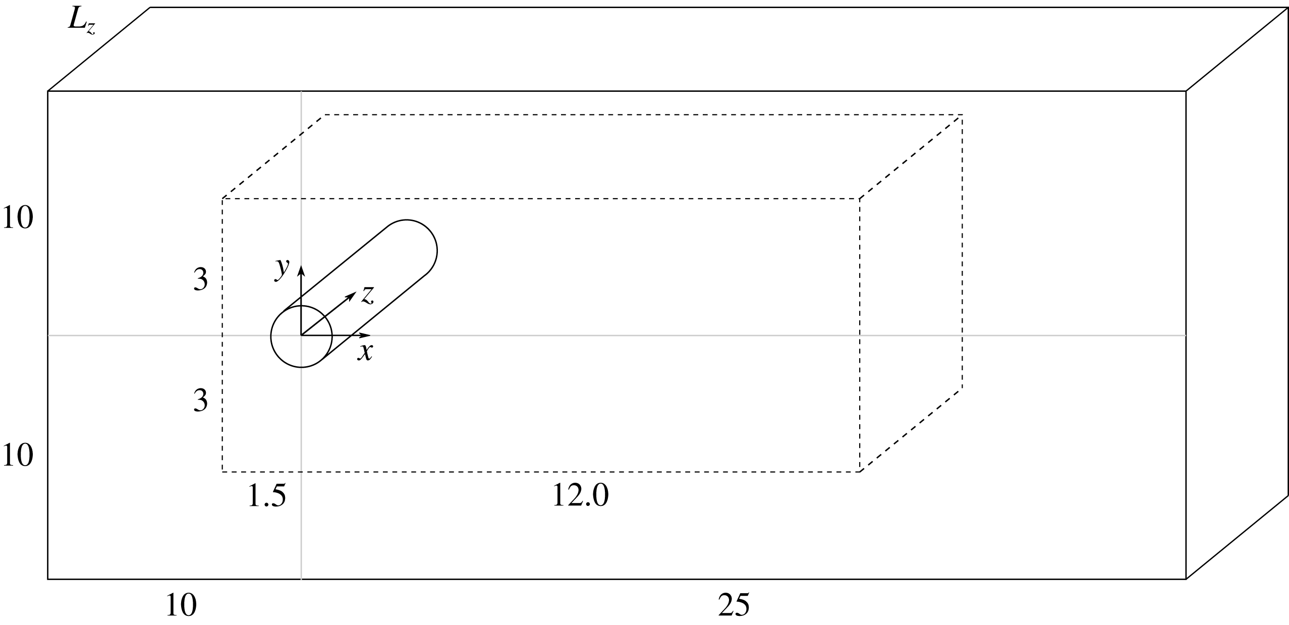
Computational domain sketch non-dimensionalised with the cylinder diameter
 $D$
. A very fine Cartesian grid domain (depicted in discontinuous lines) surrounds the cylinder and the close and mid-wake regions. A stretched rectilinear grid (depicted in solid lines) transitions from the Cartesian grid to the boundaries.

2.2 Computational details
The domain is composed of a sufficiently fine Cartesian grid for the close and mid-wake regions defined as
 $(L_{x}\times L_{y}\times L_{z})D$
, where
 $L_{x}$
and
 $L_{y}$
are the non-dimensional horizontal and vertical lengths respectively. A stretched grid is considered for the regions far from the cylinder (see figure 2). A resolution of 90 cells per diameter in all the spatial directions is chosen for the Cartesian grid subdomain. The resolution in all spatial directions is kept constant as the span is reduced.
The 3-D simulations are started from a three-dimensionalised 2-D flow snapshot. A time length of 200 units
 $(T=tU/D)$
is simulated before starting to record the flow statistics in order to achieve a statistically stationary state of the wake. The flow statistics are then recorded for a total of
 $500T$
(around 100 wake cycles). A verification and validation of the wake turbulence dynamics of the investigated test case is included in the Appendix. Finally, the turbulence statistics of the
 $L_{z}=10$
and
 $L_{z}=\unicode[STIX]{x03C0}$
cases are very similar as displayed in figure 5(a). Hence, only the
 $L_{z}=\unicode[STIX]{x03C0}$
results are displayed on the other figures for clarity.
3 Results and discussion
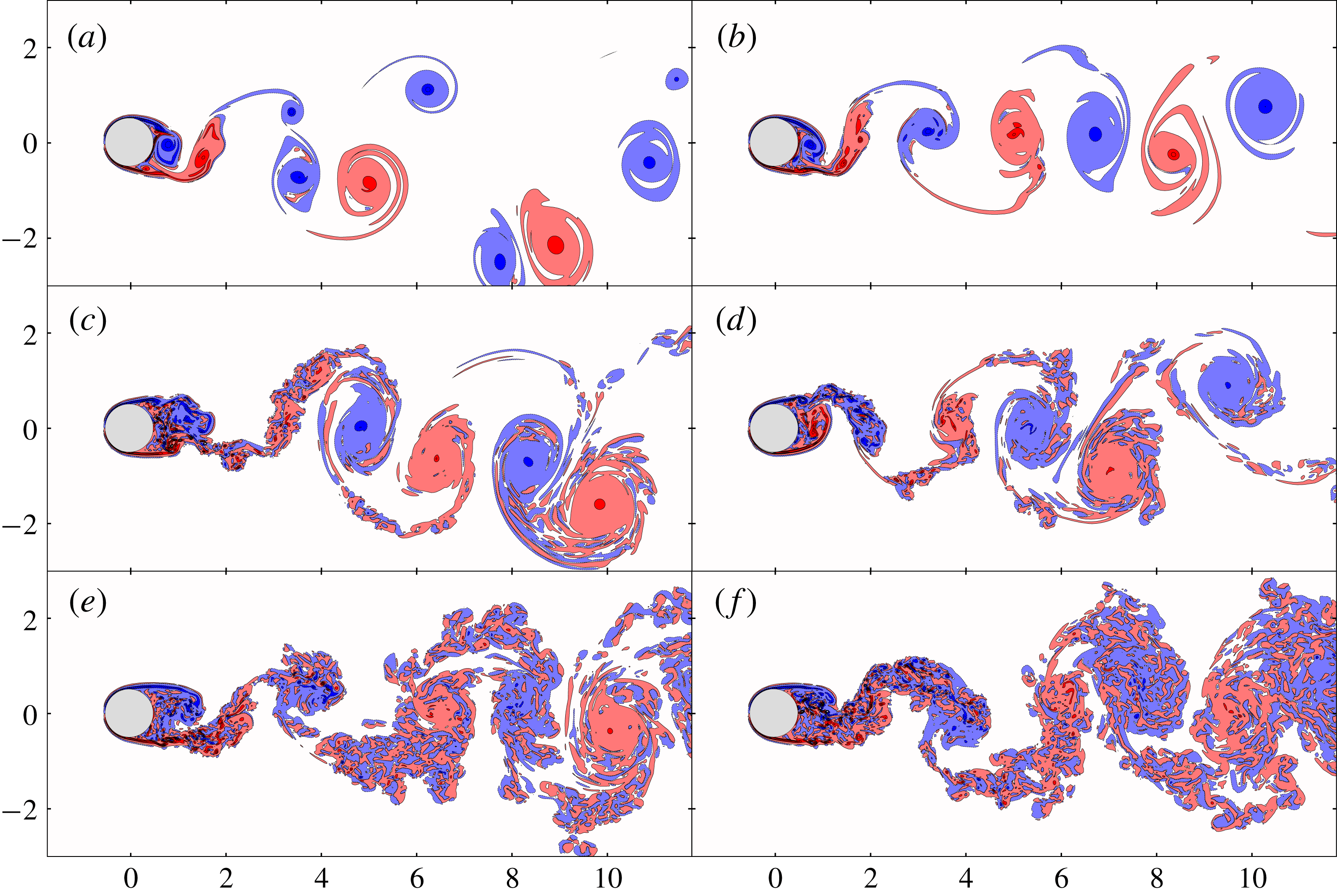
The flow field is displayed in figure 3 in terms of the instantaneous vorticity component
 $\unicode[STIX]{x1D714}_{z}$
as the span is varied. The most striking feature is how the coherence of the Kármán vortices increases as the span is reduced. However, even in highly anisotropic geometries such as
 $L_{z}=0.25$
, small-scale 3-D structures are generated from the cylinder wall.
An important result is that the two-dimensionalisation of these structures is faster (in the sense that it occurs closer to the cylinder) as the domain is constricted because of the geometry constriction and the natural rotation of the Kármán vortices. The combination of these two mechanisms as a two-dimensionalisation method is also found in Smith et al. (Reference Smith, Chasnov and Waleffe1996) and Xia et al. (Reference Xia, Byrne, Falkovich and Shats2011). For the
 $L_{z}\geqslant 1$
cases, the 3-D small-scales structures detaching from the cylinder wall are not two-dimensionalised as rapidly. In fact, it can be appreciated that only the far wake region of the
 $L_{z}=1$
case displays a coherent Kármán vortex. This means that less anisotropic geometries promote a direct TKE cascade on the wake so that the 3-D dissipative structures are still sustained far from the cylinder.
Instantaneous vorticity
 $\unicode[STIX]{x1D714}_{z}$
(red is positive, blue is negative) at the
 $z=L_{z}/2$
plane for: (a)
 $L_{z}=0$
, (b)
 $L_{z}=0.1$
, (c)
 $L_{z}=0.25$
, (d)
 $L_{z}=0.5$
, (e)
 $L_{z}=1$
, (f)
 $L_{z}=\unicode[STIX]{x03C0}$
.

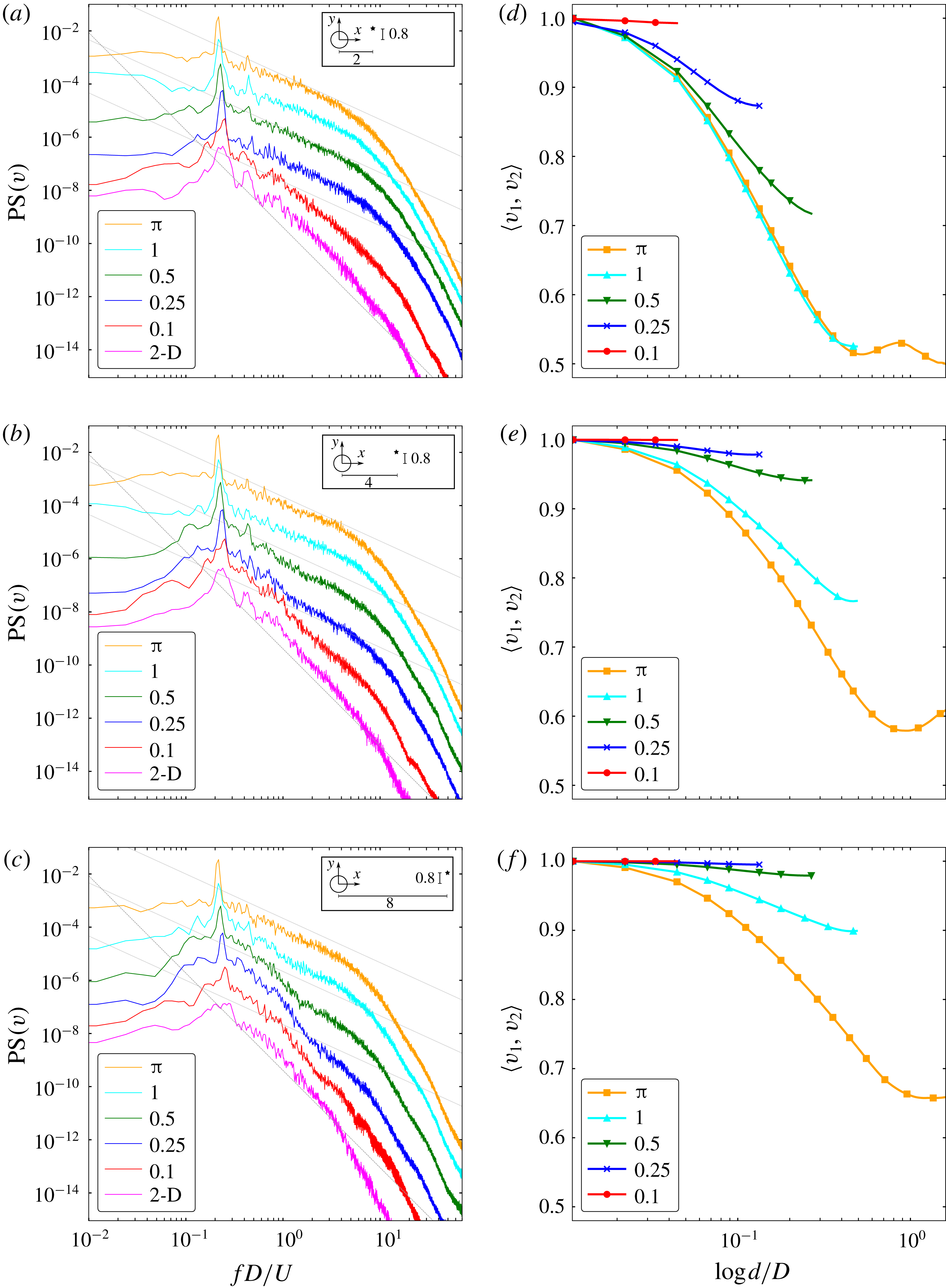
Whether the wake turbulence dynamics is two-dimensional or three-dimensional is better captured on the TKE spectra, which can be directly compared to classic turbulence theory. For this, the Taylor’s hypothesis is considered and the temporal spectrum at different points of the wake is calculated. Figure 4(a,b,c) shows the temporal power spectrum (PS) of the
 $v$
velocity component at
 $(x,y)=(2,0.8),(4,0.8),(8,0.8)$
. The Welch method (using a time signal of 500 units split in 6 parts with 75 % overlapping) has been employed to compute the spectra at 8 different points along the span for each
 $(x,y)$
point. These spectra are then averaged resulting in a single spectrum for each case.
First, note that all of the spectra display a peak around the 0.2 non-dimensional frequency corresponding to the non-dimensional Strouhal number,
 $S_{t}=f_{s}D/U$
, where
 $f_{s}$
is the vortex-shedding frequency. A smaller harmonic peak around 0.4 non-dimensional frequency is also found for the spectra at
 $(x,y)=(2,0.8),(4,0.8)$
. Second, the spectrum at the closest analysed point to the cylinder (figure 4
a) displays a 3-D turbulence behaviour with a
 $-5/3$
decay rate with the exception of the pure 2-D and the
 $L_{z}=0.1$
cases. For the latter cases, a decaying slope around
 $-11/3$
is found. These 2-D flow spectra are steeper than the
 $-3$
rate predicted by the classical 2-D turbulence theory (Kraichnan Reference Kraichnan1967) because of the interaction of the coherent large-scale Kármán vortices, in agreement with the finds of Dritschel et al. (Reference Dritschel, Scott, Macaskill, Gottwald and Tran2008) and Biancofiore (Reference Biancofiore2014). The filamentary vorticity (filaments of vorticity around the coherent vortices) is likely to be destroyed by the interaction of the large-scale vortices rather than viscous effect (specially for high
 $Re$
flows), thus limiting its range of scales. The coherent vortices induce a spiralling effect which limits the range of scales of incoherent filamentary vorticity (Gilbert Reference Gilbert1988). On the other hand, as a
 $-5/3$
decay rate is captured for the
 $L_{z}=0.25$
case, it can be argued that 3-D turbulence is being generated from the cylinder wall even for highly reduced spans.
(a–c) Vertical velocity component temporal power spectrum at different
 $(x,y)$
locations on the wake:
 $(a)=(2,0.8)$
,
 $(b)=(4,0.8)$
,
 $(c)=(8,0.8)$
. The PS lines of each case are shifted a factor of 10 for clarity and the vertical axis ticks correspond to the
 $L_{z}=\unicode[STIX]{x03C0}$
case. The dashed lines have a
 $-11/3$
slope and the dotted lines have a
 $-5/3$
slope. (d–f) Two-point correlations along
 $z$
at the same
 $(x,y)$
locations as (a–c) respectively. The correlation value for a given
 $d$
corresponds to the averaged value of the multiple correlations of pairs of points separated a distance
 $d$
along the span.

The
 $L_{z}=0.25$
and
 $L_{z}=0.5$
cases feature a decay rate that transitions from
 $-5/3$
to
 $-11/3$
as the spectra are computed further downstream from the cylinder. In particular, both cases have
 $-5/3$
slopes in figure 4(a) and
 $-11/3$
in figure 4(c), quantifying the turbulent two-dimensionalisation in the rotating wake. Also note the coexistence of both 2-D and 3-D turbulence features for the
 $L_{z}=0.25,0.5$
and
 $L_{z}=1$
cases in figures 4(b) and 4(c) respectively. The low-frequency structures behave mostly two-dimensionally (decay rate between
 $-3$
and
 $-11/3$
, resulting from the presence of less coherent 2-D structures than the pure 2-D case) up to a certain point where a
 $-5/3$
rate is briefly recovered. Hence, high-frequency structures interact in a 3-D fashion while low-frequency structures interact two-dimensionally. This finding is in agreement with Smith et al. (Reference Smith, Chasnov and Waleffe1996) and Celani et al. (Reference Celani, Musacchio and Vincenzi2010).
Additionally, two-point correlations along the span have been analysed at the same
 $(x,y)$
locations as the PS plots (figure 4
d–f). Given a distance
 $d$
along
 $z$
ranging from 0 to
 $L_{z}/2$
, the two-point correlation is calculated with the temporal signals of the vertical velocity component at multiple pairs of points (namely
 $v_{1}$
and
 $v_{2}$
) as follows,
 $$\begin{eqnarray}\langle v_{1}(\boldsymbol{x},t),v_{2}(\boldsymbol{x}+\boldsymbol{r},t)\rangle =\frac{\text{cov}(v_{1},v_{2})}{\sqrt{\text{cov}(v_{1},v_{1})\text{cov}(v_{2},v_{2})}},\end{eqnarray}$$
where the distance vector is defined as
 $\boldsymbol{r}=(0,0,d)$
. The multiple correlation coefficients for a given
 $d$
are then averaged corresponding to a data point in the plots.
Very close to the cylinder (figure 4
d), the correlation coefficient quickly decreases with increasing
 $d$
for
 $L_{z}>0.1$
. This indicates the presence of 3-D structures near the body as also noted on the velocity spectrum plot counterpart. Also, the decrease is more pronounced as the span increases. For
 $L_{z}=\unicode[STIX]{x03C0}$
, it is worth noting a local correlation coefficient maximum around
 $d\approx 0.9$
. This distance approximately corresponds to the Mode B instability wavelength
 $(\unicode[STIX]{x1D706}_{z})$
. Since the rib-like vortices associated with Mode B instability (streamwise and cross-flow vorticity) are not very well defined at this
 $Re$
regime (Chyu & Rockwell Reference Chyu and Rockwell1996), the correlation increase is not as significant as at lower
 $Re$
. Still,
 $L_{z}=\unicode[STIX]{x03C0}$
is the only case displaying such phenomena because of the spanwise boundary conditions’ periodicity, which only allow the instability to develop if
 $L_{z}>\unicode[STIX]{x1D706}_{z}$
(the
 $L_{z}=1$
case might be too critical to display such phenomena considering also its intermittent nature). The correlation coefficient increases when calculated further downstream as shown in figures 4(e) and 4(f), evidencing again the wake two-dimensionalisation.
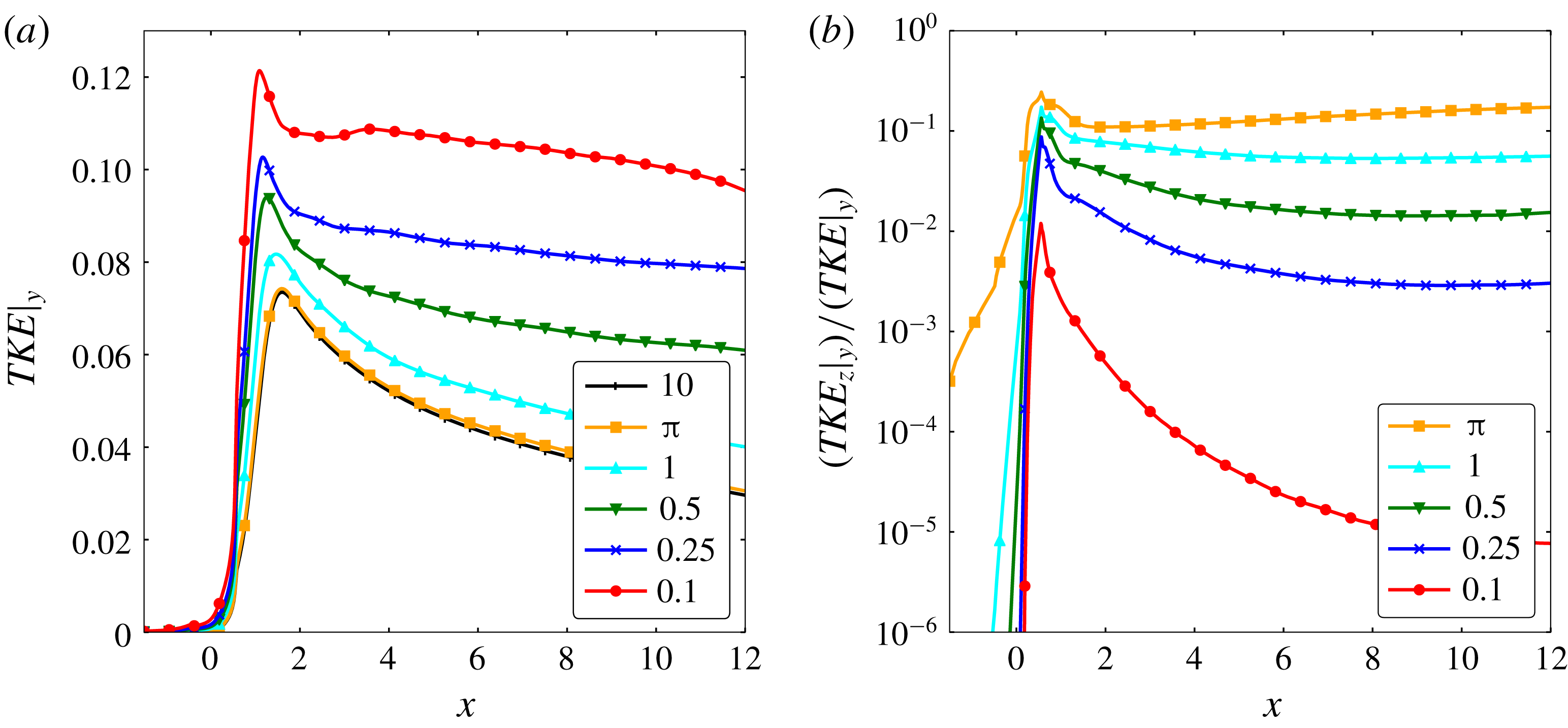
TKE spatial plots. The TKE is computed from the normal Reynolds stresses and averaged on the vertical direction: (a) total TKE, (b) ratio of the spanwise component
 $\overline{w^{\prime }w^{\prime }}$
over the total TKE.

In summary, the transition to a 2-D wake is found at a certain point along the wake on all the cases with
 $L_{z}\leqslant 1$
. The combination of the large-scale rotation from the Kármán vortices plus the geometry constriction is mainly responsible for this phenomenon. The main physical mechanism differing among the compared cases is the ability of the flow to develop Mode B-like 3-D structures in the wake as a result of a sufficiently long span. The current
 $Re$
regime is characterised by a transition to turbulent flow at the shear layer (i.e. the TrSL2 regime) as reported in Bloor (Reference Bloor1964) and Kourta et al. (Reference Kourta, Boisson, Chassaing and Ha Minh1987). We argue that when the span is too short for the Mode B instability to develop and thereby sustain these 3-D turbulent structures, the stratification effect of the Kármán vortices leads to the more coherent and energised wake seen in figure 4(d–f).
Next, the TKE along the
 $x$
direction, the Lumley triangle of turbulence and the ratio between the vortex-stretching and advection terms are examined to further support the observed phenomena. The TKE is defined as,
 $$\begin{eqnarray}\text{TKE}={\textstyle \frac{1}{2}}(\overline{u^{\prime }u^{\prime }}+\overline{v^{\prime }v^{\prime }}+\overline{w^{\prime }w^{\prime }}),\end{eqnarray}$$
where
 $\overline{\cdot }$
denotes a time average plus a spanwise average and the subscript
 $\cdot ^{\prime }$
denotes a fluctuating quantity such as
 $a^{\prime }=a-\overline{a}$
. The six components of the Reynolds stress tensor
 $\overline{u_{i}^{\prime }u_{j}^{\prime }}$
have been computed using the following relation,
 $$\begin{eqnarray}\overline{a^{\prime }b^{\prime }}=\overline{ab}-\overline{a}\overline{b}.\end{eqnarray}$$
Figure 5 shows the streamwise spatial distribution of the TKE averaged along the
 $y$
direction from
 $-L_{y}/2$
to
 $L_{y}/2$
(noted as
 $\cdot |_{y}$
). From a general point of view, it can be observed that the total TKE (figure 5
a) peaks right after the recirculation region noting that the latter increases slightly with the span. Also, the total TKE increases as the span is reduced because of the 2-D vortex-merging processes that generate larger and more energised vortical structures. The contribution of the spanwise normal stress to the total TKE increases with the span as shown in figure 5(b). Also, a decay of
 $\overline{w^{\prime }w^{\prime }}$
right after being generated from the cylinder wall can be noted and it becomes faster as the span is constricted.
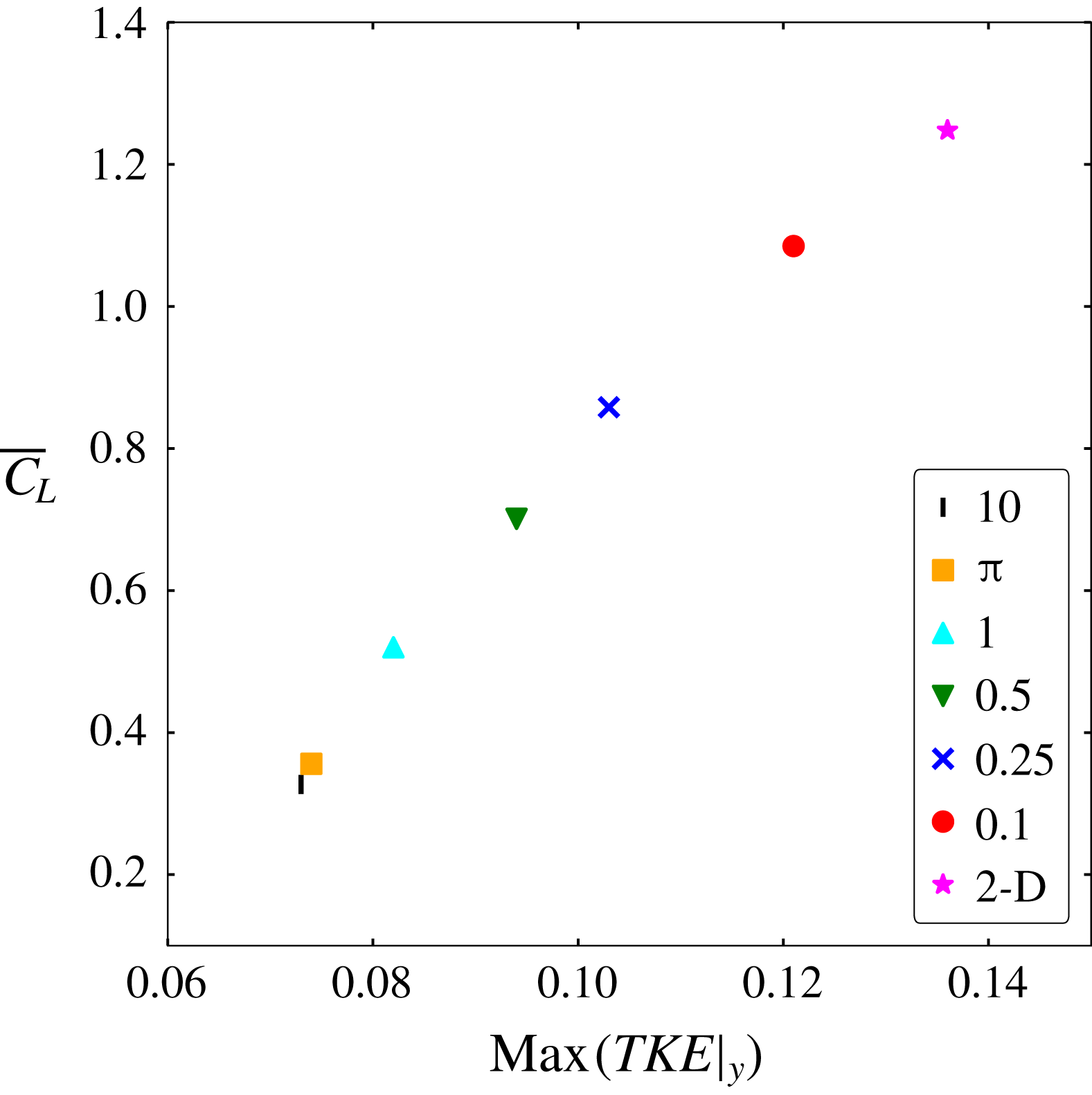
The effect of the span on the TKE compared to the lift coefficient root mean square (r.m.s.) value
 $(\overline{C}_{L})$
displays a quasi-linear relation as shown in figure 6. Note that the drop on both values is more sensitive to the span constriction at the range where both 2-D and 3-D turbulence dynamics co-exist, i.e.
 $0.25\leqslant L_{z}\leqslant 1$
. On the other hand, a very small change of both values can be appreciated when 3-D turbulence fully dominates the wake, i.e.
 $L_{z}\geqslant \unicode[STIX]{x03C0}$
. Furthermore, as shown in figure 5(a), highly constricted domains yield large values of TKE because of the energised 2-D large-scale vortical structures present at the wake. Even when small-scale 3-D structures are present in the close wake region and coexist with the large 2-D structures, the values of both the TKE and the
 $\overline{C}_{L}$
spike.
Effect of the span constriction on the TKE and the
 $\overline{C}_{L}$
. The latter is calculated as
 $\overline{C}_{L}=|2F_{y}/(\unicode[STIX]{x1D70C}U^{2}DL_{z})|_{rms}$
, where
 $F_{y}$
is the vertical lift force and
 $\unicode[STIX]{x1D70C}$
is the constant fluid density.

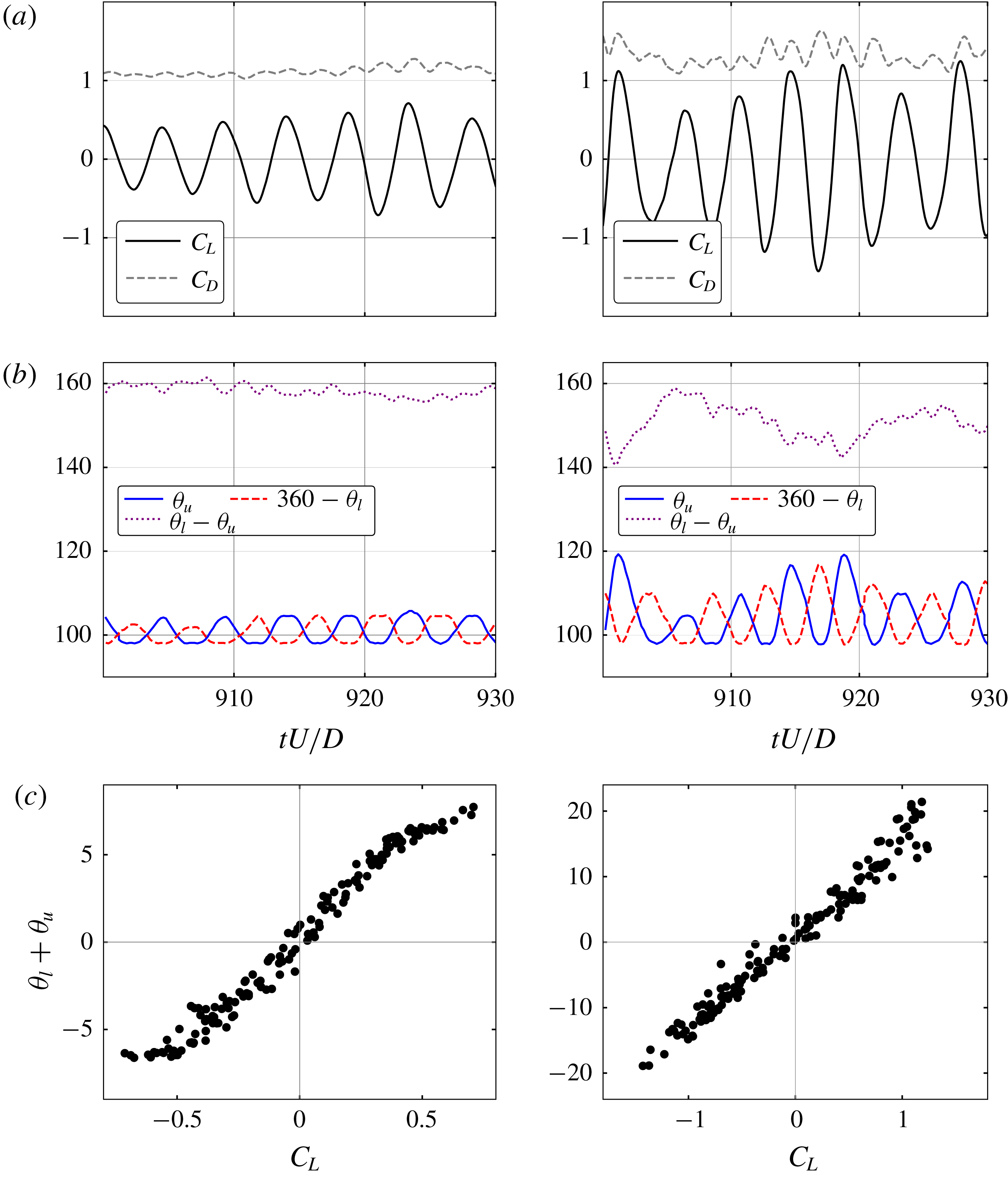
(a)
 $C_{L}$
and
 $C_{D}$
temporal signals. The latter is calculated as
 $C_{D}=2F_{x}/(\unicode[STIX]{x1D70C}U^{2}DL_{z})$
and the former as detailed in figure 6 (without the r.m.s. norm). (b) Upper
 $\unicode[STIX]{x1D703}_{u}$
and lower
 $\unicode[STIX]{x1D703}_{l}$
separation angles temporal signal. The separation angle is calculated from the front stagnation point of the cylinder to the free-shear layer separation point (vorticity practically 0 at the wall). (c) Correlation between the lift coefficient and the difference between
 $\unicode[STIX]{x1D703}_{u}$
and
 $360-\unicode[STIX]{x1D703}_{l}$
. Left:
 $L_{z}=\unicode[STIX]{x03C0}$
. Right:
 $L_{z}=0.5$
.

In figure 7, the temporal signals of the lift and drag coefficients as well as the upper and lower separation angles of the free-shear layer are displayed for the
 $L_{z}=0.5$
and the
 $L_{z}=\unicode[STIX]{x03C0}$
cases. The oscillation of the separation points increases as the span is constricted inducing larger forces on the cylinder. A very high correlation of the upper and lower separation points angle with the lift coefficient is shown as well. Again, the lack of the Mode B instability on the constricted cases yields more coherent 2-D vortical structures in the near wake region. Therefore, the small-scale 3-D structures which normally dissipate most of the kinetic energy in 3-D turbulence are not present leading to high-intensity vortices. This can be quantified by the enstrophy (
 $\unicode[STIX]{x1D6FA}$
) of the span-averaged spanwise vorticity in the near wake region
 ${\mathcal{D}}$
(
 $x\in [0.55,2.1]$
,
 $y\in [-0.8,0.8]$
), which is time averaged for the same temporal length as the body forces signals as follows,
 $$\begin{eqnarray}\unicode[STIX]{x1D6FA}=\int _{{\mathcal{D}}}\frac{1}{t_{2}-t_{1}}\int _{t_{1}}^{t_{2}}\frac{1}{L_{z}}\int _{0}^{L_{z}}\unicode[STIX]{x1D714}_{z}^{2}\,\text{d}z\,\text{d}t\,\text{d}{\mathcal{D}}.\end{eqnarray}$$
It can be observed in table 1 that the enstrophy increases as the span is reduced, which can be understood as an increase of the rotational energy of the flow.
Near body enstrophy as defined in (3.4) for the different span cases.
 $\unicode[STIX]{x1D6FA}_{\unicode[STIX]{x03C0}}$
is the enstrophy of the
 $L_{z}=\unicode[STIX]{x03C0}$
case.

The highly energised coherent vortices forming at the near wake region for the constricted cases induce a larger convective force on the free-shear layer. This translates to the large oscillations observed in figure 7 and, ultimately, to the forces induced on the cylinder. With this, it can be argued that the coherent 2-D structures have a greater impact on the forces induced to the cylinder than the 3-D small-scale structures when both are present.
Lumley & Newman (Reference Lumley and Newman1977) proposed the Lumley triangle of turbulence which provides a way to classify the anisotropic state of turbulence. The anisotropy property of the Reynolds stress tensor can be extracted with,
 $$\begin{eqnarray}\unicode[STIX]{x1D623}_{ij}=\frac{\overline{u_{i}^{\prime }u_{j}^{\prime }}}{\overline{u_{k}^{\prime }u_{k}^{\prime }}}-\frac{1}{3}\unicode[STIX]{x1D6FF}_{ij},\end{eqnarray}$$
where
 $\unicode[STIX]{x1D6FF}$
is the Kronecker delta and
 $\unicode[STIX]{x1D623}_{ij}$
is the anisotropic Reynolds stress tensor (which evidently vanishes for isotropic turbulence). This dimensionless and traceless tensor has two non-zero invariants,
 $II=-\unicode[STIX]{x1D623}_{ij}\unicode[STIX]{x1D623}_{ji}/2$
and
 $III=\unicode[STIX]{x1D623}_{ij}\unicode[STIX]{x1D623}_{jk}\unicode[STIX]{x1D623}_{ki}/3$
. These invariants are often rewritten as
 $\unicode[STIX]{x1D702}^{2}=-II/3$
and
 $\unicode[STIX]{x1D709}^{3}=III/2$
to better appreciate the nonlinear behaviour of the trajectories of return to isotropy of homogeneous turbulence (Choi & Lumley Reference Choi and Lumley2001). It has been shown that all the possible turbulence states are mapped within the triangle (Lumley & Newman Reference Lumley and Newman1977; Lumley Reference Lumley1978).
The different states of turbulence are classified in the triangle as follows: the top right elbow indicates a one-dimensional (or one component) state with a single non-zero eigenvalue (the eigenvalues can be understood in physical terms as the normal stresses in the principal axes of the anisotropic Reynolds stress tensor). The top left elbow indicates a 2-D isotropic state where one eigenvalue vanishes and the two remaining are equal. The top curve connecting the elbows indicates a 2-D turbulence state where one eigenvalue vanishes and the addition of the two remaining eigenvalues is constant. The left and right straight lines correspond to a negative or positive
 $(\unicode[STIX]{x1D709})$
axisymmetric state since one eigenvalue is smaller than the other two (which are equal) or greater than the other two (which are equal) respectively. Finally, the
 $(0,0)$
point indicates 3-D isotropic turbulence since all of the anisotropic tensor eigenvalues vanish.
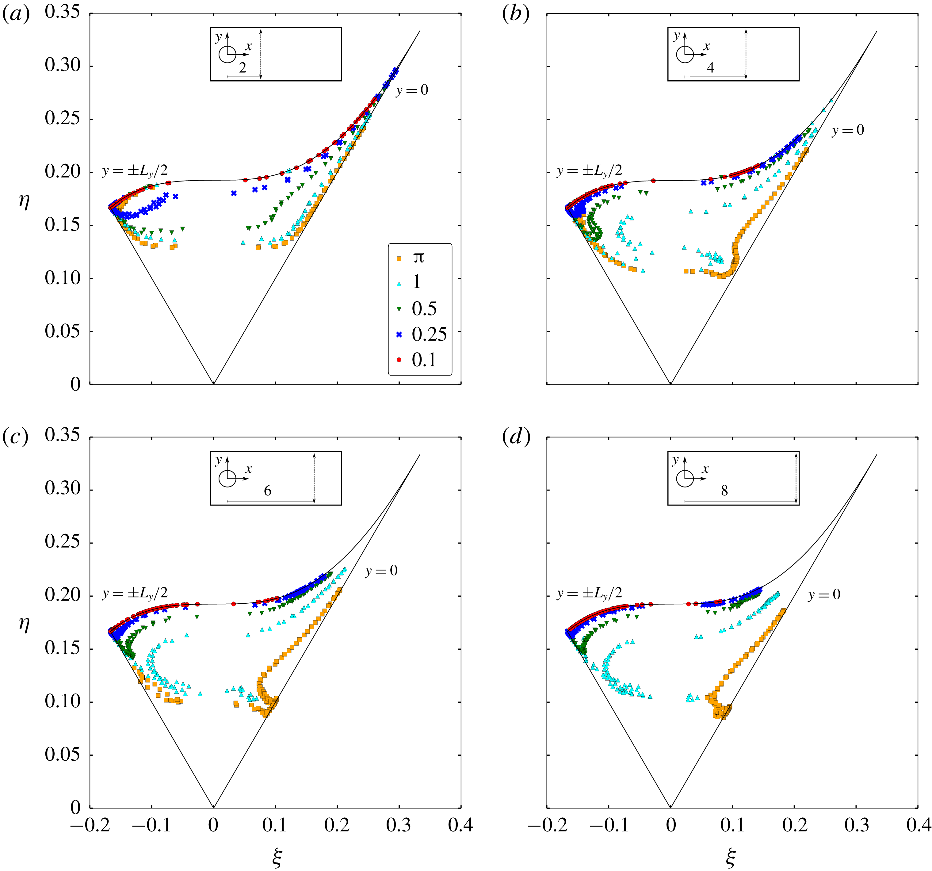
Lumley’s triangle constructed across the wake width at: (a)
 $x=2$
, (b)
 $x=4$
, (c)
 $x=6$
, (d)
 $x=8$
.

Figure 8 displays the Lumley triangle constructed across the wake width at different
 $x$
locations. Hence, every point in the triangle corresponds to a point in the domain and the collection of points for each case represents the collection of vertically aligned points in the domain at different
 $x$
locations on the wake. It can be appreciated that all of the points are located within the triangle, therefore all of computed Reynolds stresses are realisable (i.e. have positive and real eigenvalues). In general, most of the cases transition from one state to another state of turbulence across the wake width. Only for the almost 2-D case
 $(L_{z}=0.1)$
, the state of turbulence is always 2-D (or two-component), since
 $\overline{w^{\prime }w^{\prime }}$
is effectively negligible everywhere.
As the triangle is constructed further downstream on the wake, the trajectories (or collection of points) of the
 $L_{z}=0.25$
and
 $L_{z}=0.5$
cases move closer to the 2-D turbulence state location (upper curve). This emphasises once again the wake two-dimensionalisation caused by the large-scale vortical structures on cases with critical span which contain a cross-over of 2-D and 3-D turbulence, as shown in previous results. In contrast, the
 $L_{z}=1$
and
 $L_{z}=\unicode[STIX]{x03C0}$
cases remain approximately at the same
 $\unicode[STIX]{x1D702}$
region showing that the two-dimensionalisation is not as effective.
Additionally, the trajectories present a negative axisymmetric almost two-component state for the locations far from the wake centreline, i.e. the location close to
 $y=\pm L_{y}/2$
, since one of the normal turbulent stresses
 $\overline{w^{\prime }w^{\prime }}$
is smaller than the others. On the centreline,
 $\overline{v^{\prime }v^{\prime }}$
is larger than the other stresses, causing a shift to the positive axisymmetric state.
A comparison of the different cases at the same
 $x$
location also shows a more noticeable 2-D turbulence state as the span is constricted. This difference is less noticeable close to the cylinder (figure 8
a), where even the
 $L_{z}=0.5$
case trajectory resembles the
 $L_{z}=\unicode[STIX]{x03C0}$
case. Again, this evidences that 3-D turbulence is present close to the wall even in considerably constricted cases.
Consider now the vorticity transport equation (VTE) which can be written as,
 $$\begin{eqnarray}\unicode[STIX]{x2202}_{t}\unicode[STIX]{x1D74E}+\boldsymbol{u}\boldsymbol{\cdot }\unicode[STIX]{x1D735}\unicode[STIX]{x1D74E}=\unicode[STIX]{x1D74E}\boldsymbol{\cdot }\unicode[STIX]{x1D735}\boldsymbol{u}+Re^{-1}\unicode[STIX]{x1D6FB}^{2}\unicode[STIX]{x1D74E},\end{eqnarray}$$
where
 $\unicode[STIX]{x1D74E}(\boldsymbol{x},t)=(\unicode[STIX]{x1D714}_{x},\unicode[STIX]{x1D714}_{y},\unicode[STIX]{x1D714}_{z})$
is the vorticity vector field defined as
 $\unicode[STIX]{x1D74E}=\unicode[STIX]{x1D735}\times \boldsymbol{u}$
. The vortex-stretching term,
 $\unicode[STIX]{x1D74E}\boldsymbol{\cdot }\unicode[STIX]{x1D735}\boldsymbol{u}$
, is often pointed to as the term responsible for the direct energy cascade of the TKE. The stretching of a vortex tube causes a reduction on its diameter while increasing the rotation speed of the vortex by conservation of angular momentum. This term vanishes in the 2-D formulation of the VTE since the stretch of the vortex tube is perpendicular to the plane of rotation. From this mathematical and physical difference, different turbulence dynamics is captured in 2-D or 3-D computations and, therefore, 3-D turbulence can be directly linked to this term.
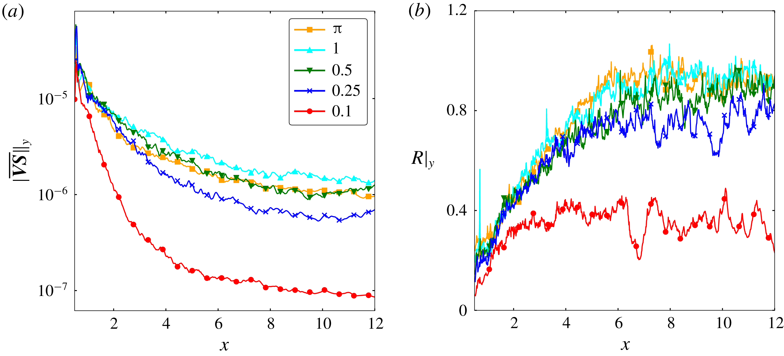
Figure 9 displays the modulus of the mean vortex-stretching term and its ratio
 $R$
with the mean vortex-advecting term. These quantities are averaged in the vertical direction. In figure 9(a), it can be observed that the vortex-stretching term decays faster while moving downstream from the cylinder for cases with shorter span. The vortex-stretching decay demonstrates again the two-dimensionalisation of the flow by the large-scale vortices. The ratio
 $R$
in figure 9(b) shows that the vortex-advecting term decays faster (because of the wake momentum deficit) than the vortex-stretching term along the streamwise direction up to
 $x=6$
where the ratio is kept constant. It can also be observed that the vortex-stretching term becomes as important as the vortex-advecting term with increasing span.
(a) Modulus of the mean vortex-stretching term averaged along the vertical direction. (b) Ratio between the modulus of the mean vortex-stretching term and the modulus of the mean vortex-advecting term averaged along the vertical direction.

4 Conclusion
The span effect on the turbulence dynamics of a flow past a circular cylinder at
 $Re=10\,000$
has been investigated using spectra and two-point correlations at different locations in the domain, the TKE along the wake, the separation points, the Lumley triangle of turbulence and the mean vortex-stretching term of the VTE. It has been shown that 3-D turbulence is present even for highly constricted cases (for example
 $L_{z}=0.25$
) which is generated by the cylinder wall (figure 4
a). However, the small-scale structures rapidly get two-dimensionalised by the large-scale Kármán vortices when the span is 50 % of the diameter or less. This is linked to the Mode B instability wavelength being longer than the periodic span, in agreement with Bao et al. (Reference Bao, Palacios, Graham and Sherwin2016). Since the Mode B instability helps sustaining the turbulent structures advected from the shear layer, the lack of it prevents large-scale 3-D structures to be created and less dissipative structures can be sustained. In this scenario, 2-D turbulence takes over and dominates the wake dynamics creating larger, stronger and more coherent vortices. Ultimately, the coherent and energised vortical structures induce a larger convective force on the free-shear layer. This translates to larger oscillations and, finally, higher forces on the cylinder.
The flow turbulence transition from three-dimensional to two-dimensional caused by a geometry constriction found in this work is in agreement with the physical mechanisms described in the obstacle-free turbulence work of Smith et al. (Reference Smith, Chasnov and Waleffe1996), Celani et al. (Reference Celani, Musacchio and Vincenzi2010) and Biancofiore (Reference Biancofiore2014). In the present study with solid boundaries, the main difference is found on the presence of small-scale 3-D turbulence even in highly constricted geometries
 $(L_{z}=0.25)$
which leads to a coexistence of 2-D and 3-D turbulence close to the cylinder wall. This is observed not only in the
 $L_{z}=0.25$
case but also for the
 $L_{z}=0.5$
and
 $L_{z}=1$
cases as shown in figures 4(b) and 4(c) respectively. Note that the cross-over between 2-D and 3-D turbulence dynamics arises at different points in the spatial domain depending on the span length. The shorter the span, the closer to the cylinder it takes place, evidencing that the wake two-dimensionalisation transitions at different locations in function of the domain geometric anisotropy.
On the other hand, a very rapid two-dimensionalisation is found in the present cases because of the natural large-scale rotation motion of the Kármán vortices. A large-scale rotation as a mechanism of two-dimensionalisation has been also found in other works such as Smith et al. (Reference Smith, Chasnov and Waleffe1996) and Xia et al. (Reference Xia, Byrne, Falkovich and Shats2011). These two mechanisms combined yield to a rapid transition from the 3-D to 2-D turbulence dynamics when the span is shorter than the Mode B instability wavelength.
Acknowledgements
The authors acknowledge the use of the IRIDIS High Performance Computing Facility, and associated support services at the University of Southampton, in the completion of this work. The authors also acknowledge the support of the Singapore Agency for Science, Technology and Research (A*STAR) Research Attachment Programme (ARAP) as a collaboration between the A*STAR Institute of High Performance Computing (IHPC) and the Faculty of Engineering and the Environment of the University of Southampton.
Appendix
A grid convergence study has been conducted in order verify the correct implementation of the governing equations and to show that the selected grid resolution and averaging time length is suitable for a proper analysis. Three grids with different resolution
 $(\unicode[STIX]{x1D6E5})$
designed as shown in figure 2 have been investigated for the
 $L_{z}=\unicode[STIX]{x03C0}$
case (see details in table 2). The refinement ratio is
 $\sqrt{2}$
.
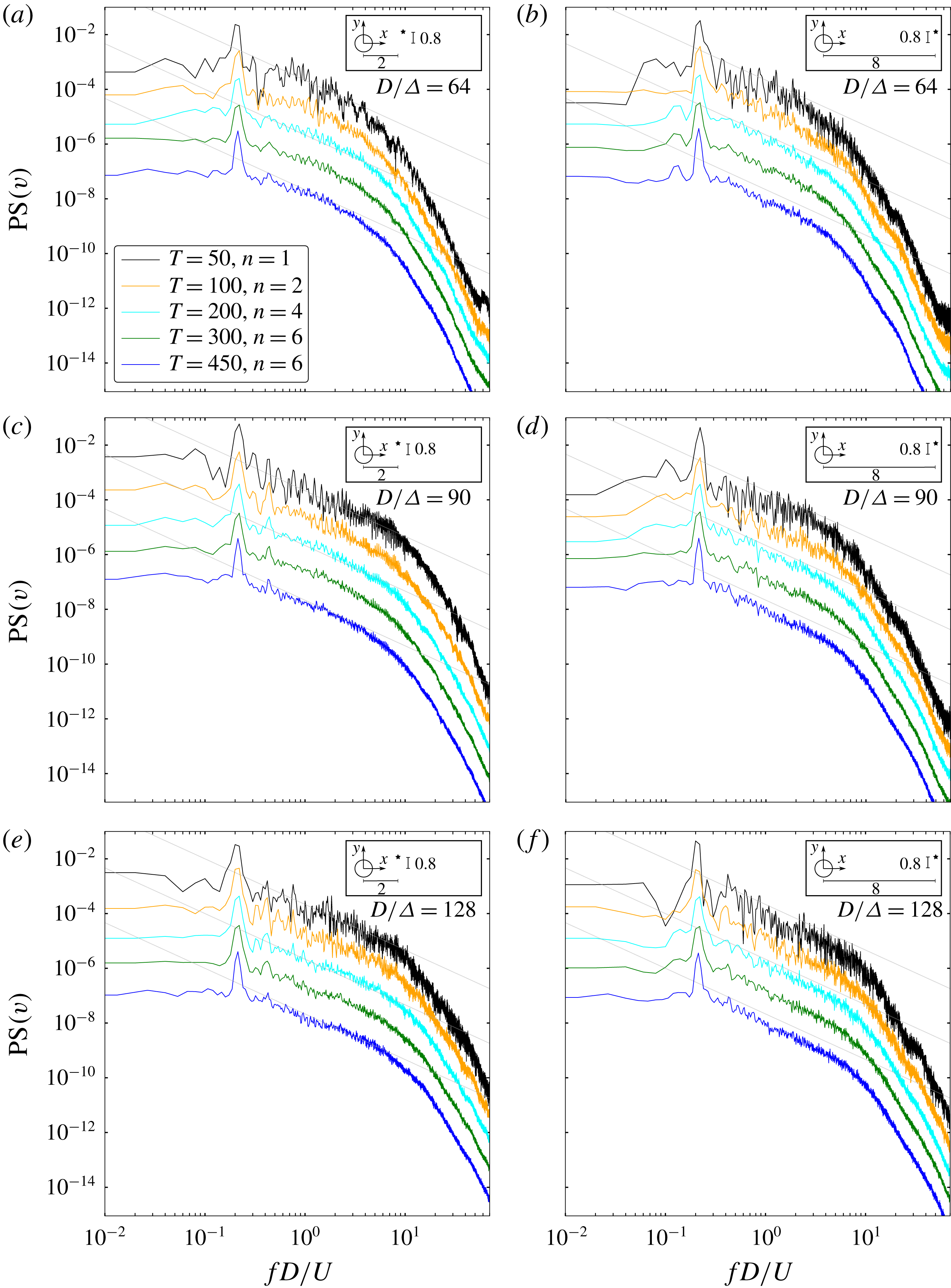
Vertical velocity component temporal power spectra at the close (a,c,e) and far (b,d,f) wake regions. The coarse, medium and fine grid results are displayed at the first, second and third row respectively. The spectra are shifted by a factor of 10 and the vertical axis ticks correspond to the
 $T=50$
case. The number of the time signal splits selected for the Welch method (
 $n$
) ensures a minimum of
 $50T$
per split (at least 8 times larger than the lowest frequency of interest, i.e. the shedding frequency which is around
 $5T$
) and a maximum of 6 splits per total time signal. The dotted line corresponds to a
 $-5/3$
slope.

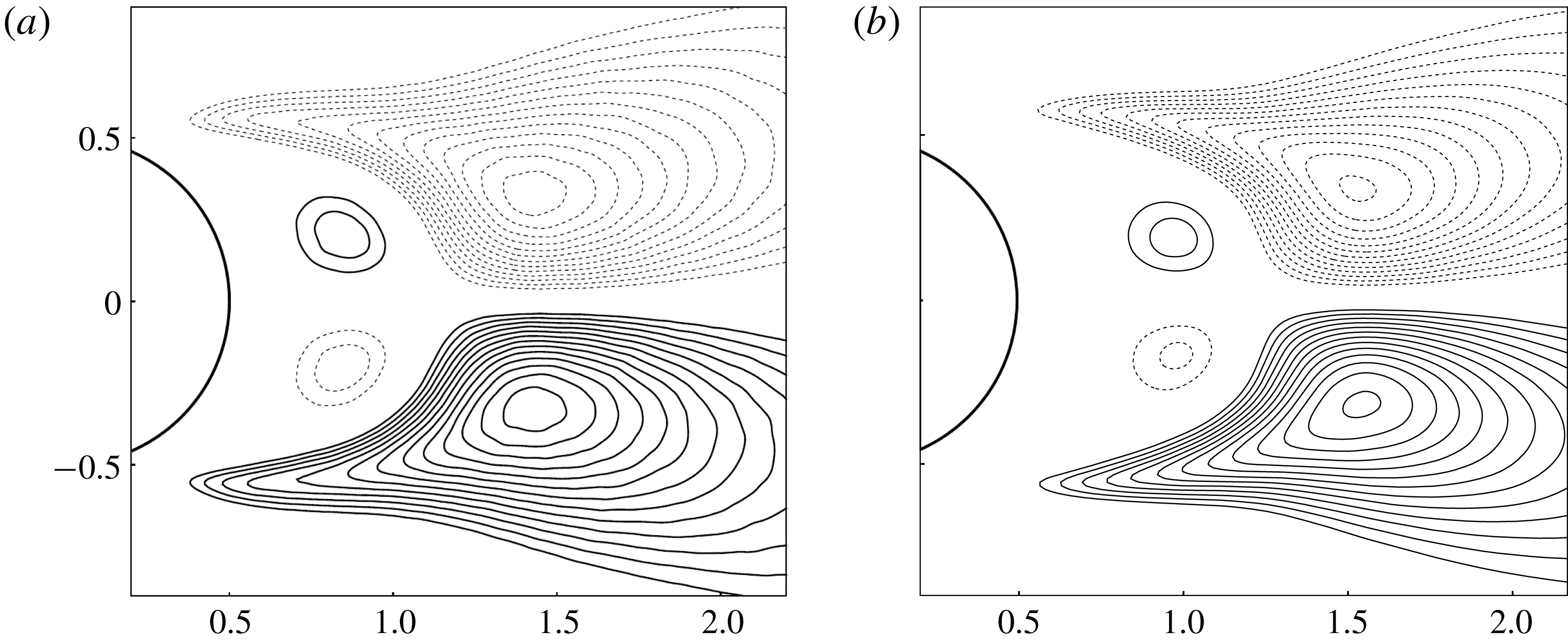
Comparison of the Reynolds shear stress
 $\overline{u^{\prime }v^{\prime }}$
between: (a) direct numerical simulation data from Dong & Karniadakis (Reference Dong and Karniadakis2005) and (b) present solver. The contour level criterion is the same as the reference data:
 $|\overline{u^{\prime }v^{\prime }}|_{min}=0.03$
and
 $\unicode[STIX]{x0394}\overline{u^{\prime }v^{\prime }}=0.01$
. Positive and negative levels are noted with continuous and dashed lines respectively.

The quantities of interest of the present work are the turbulence statistics arising from time and spatial averages. Because of this, we need to ensure that the presented results are statistically stationary and have converged in spatial resolution terms. The velocity temporal power spectrum constructed analogously to figure 4 at the
 $(2,0.8)$
and
 $(8,0.8)$
locations is used with this purpose. The spectrum produced by investigated grids is shown for different time signal lengths in figure 10.
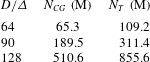
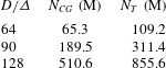
Details of the three different grids ranging from coarse (
 $D/\unicode[STIX]{x1D6E5}=64$
, i.e. 64 cells per diameter) to fine (
 $D/\unicode[STIX]{x1D6E5}=128$
) for
 $L_{z}=\unicode[STIX]{x03C0}$
.
 $N_{GC}$
refers to the total number of cells (in millions) for the Cartesian grid subdomain.
 $N_{T}$
refers to the total number of cells (in millions).
At the near wake region, the coarse grid shows a converged spectrum (
 $-5/3$
inertial subrange decay) for time signals longer than
 $200T$
. A similar behaviour is captured with the medium grid, which shows a converged spectrum for time signals longer than
 $100T$
and the resulting inertial subrange accommodates more frequencies. In the far wake region, the coarse grid presents slightly steeper spectra than at the close wake region. This can be caused by an insufficient resolution in span, which would induce a two-dimensionalisation effect. On the other hand, the medium grid still presents converged spectra for time signals longer than
 $100T$
. The fine grid leads to results very similar to the medium grid. Hence, it is shown that using the medium grid with simulation times over
 $100T$
(
 $500T$
is used in the results presented in this work) provides statistically stationary results both in the close and far wake regions.
To validate the wake turbulence statistics, the Reynolds shear stress
 $\overline{u^{\prime }v^{\prime }}$
has also been qualitatively analysed. It can be observed in figure 11 that the shear stress predicted by the present solver is in very good agreement with the direct numerical simulation data from Dong & Karniadakis (Reference Dong and Karniadakis2005), with just a slight shift of the field structures on the streamwise direction. All positive and negative regions are correctly captured which display an antisymmetric pattern with respect to the centreline of the wake.