1. INTRODUCTION
A typical polling system consists of a number N of queues attended by a single server. There exists a huge body of literature on polling systems, starting in 1957 [17,18]. Since then, polling systems have been used extensively in communication networks as well as manufacturing systems. In this article, we consider a polling system with N queues with infinite buffers. Time is slotted and the slot durations are either deterministic with unit size or exponentially distributed with mean one. In each queue, one customer arrives in each time slot, we assume that its required service time is queue dependent, it is a fixed amount in the deterministic polling model, and it is exponentially distributed in the exponential model. For the deterministic model, we also consider the model with fluid input. There is one server, and at the beginning of each time slot the decision has to be made about which queue is being served during the next time slot; we assume zero switching times, as is usual in the performance analysis of communication networks. The service discipline is first in–first out for each queue and it is work-conserving. The control of the server is an open-loop control, which means that the decision about which queue is to be served in the next time slot is independent of the actual workloads in the nodes. The open-loop polling sequence is an infinite sequence where its nth element gives the queue that is served during the nth time slot. We derive an efficient algorithm for computing the optimal open-loop polling sequence with the objective being the sum of the average workloads in the queues for the deterministic and for the exponential polling model with N = 2 queues. We exploit the theory on multimodularity of the average workload and the optimality of regular sequences as it has been derived in recent work (see [1,2]). It follows from this theory that for N = 2 queues, the optimal polling policy assigns time slots to the first queue (service sequence of the first queue, as we will call it) as a regular sequence, say with density

(and the service sequence for the second queue is also regular, with density

). As we show in Appendix A, the sum (in general of any linear combination) of the average workloads in both queues, say B(d1,d2), is a convex function of the densities (d1,d2) if the service sequences are regular for both queues. Our algorithms compute this convex function for the deterministic and exponential models. Moreover, the optimal densities

are obtained for both models.
In Sections 2–4 we analyze the two deterministic models with discrete and fluid input. For fixed densities (d1,d2), the average workloads in both queues become independent of each other and the average workloads can be studied separately. In Section 3 the average workload for one queue with a regular service sequence as a function of its density is analyzed; it is shown that it is a convex piecewise-linear function. Using results from number theory, we derive explicit formulas for the average workload in the case that the service density is a best approximation point of the input rate. With the use of the continued fraction expansion of the input rate we then derive an efficient algorithm for calculating the average workload for any density. Doing these calculations for both queues gives an efficient algorithm for calculating mind1+ d2=1 B(d1,d2), which provides the exact optimal polling policy. In Section 4 we illustrate the algorithm with numerical experiments. Also in Section 4 we derive results on the structure of the optimal policy. We prove that for deterministic polling systems with N ≥ 2 queues and rational input rates, there is always an optimal policy that is periodic.
In Appendix B, the algorithm for calculating the optimal polling sequence for the exponential system is derived. The sum of the workloads in both queues is again a convex function in the densities (d1,d2). Using the Kernel method, the exact optimal policy in open loop is computed in an efficient way.
There is extensive literature on the many variants of controlled polling systems (see [6,22]). In several articles [4,5,15] an algorithm is derived for calculating efficient visit orders to the queues, also called polling tables. In [12] the exponential polling model is converted to a Markov decision chain with no state information, and an algorithm to compute a nearly optimal polling policy is given. In [7] a heavy-traffic averaging principle is derived. To the knowledge of the authors, no algorithm for computing the exact optimal polling sequence is available in the literature. Also, it seems that our structural results are new. Since a polling can be seen as a server routing model, there is a duality with the customer routing model. The authors have studied the latter model recently (for the deterministic model, see [2,14], and for the exponential model, see [10]). The results are similar; both cases exhibit a fractal behavior. However, there also exist subtle differences that are pointed out in this article, mainly due to the fact that a polling system has several arrival processes.
2. DESCRIPTION OF DETERMINISTIC POLLING SYSTEMS
We consider a polling model in which queues are served by one server, which serves at a constant rate of 1. We assume that the input to the queues is deterministic, but we consider two slightly different models. In the first model the input to queue i, i = 1,2,…, N, is discrete and in fact we assume for i = 1,2,…, N that at all of the integer times T = 0,1,2,…, a job with constant workload λi arrives in queue i. In the second model we assume that the workload input to queue i, i = 1,2,…, N, is fluid and flows in with constant rate λi.
In both models we assume that at all of the integer times T = 0,1,2,…, a queue is chosen to be served by the server for the next time unit. So, in the case of N queues numbered 1,2,…, N, the polling policy can be described by the infinite sequence U = (U1,U2,…), where Un is the queue to be served by the server during the time interval [n − 1,n]. For both models we describe the system with N queues by the N-dimensional vector λ := (λ1,λ2,…, λN). An infinite sequence U corresponding to a polling policy for such a system is a so-called word on the alphabet {1,2,…, N} (see [14,16]). The set of all words on the alphabet {1,2,…, N} (corresponding to all of the possible polling policies for some λ system) is denoted by [Ascr ](N).
For i = 1,2,…, N and

let Vi(t) be the (remaining) workload in queue i at time t. Then the long-run average workload in queue i is given by the Cesaro integral

For U ∈ [Ascr ](N) for i = 1,2,…, N, we define an infinite sequence ui = (u1i,u2i,…) of zeros and ones by uni = 1 if Un = i and uin = 0 if Un ≠ i. We call such a sequence of zeros and ones, corresponding to the server assignment for one queue, a short service sequence. This in contrast to Chapter 9 of [2] and [1], where such a sequence is called a vacation sequence. Note that given the fact that we consider a model with fluid or discrete input, the value of Bi for a given queue i depends only on the arrival rate λi in the queue and the service sequence ui for this queue.
For both the discrete model and the fluid model the objective of the polling is to minimize the total long-run average workload, which is given by

where U is the polling policy. So, a polling policy U′ is called optimal for a given λ system (either for the discrete or the fluid model) if B(U′) = minU∈[Ascr ](N) B(U). The minimal total long-run average workload for some λ system is given by

3. ON THE AVERAGE WORKLOAD IN A SINGLE QUEUE
In this section we consider a single queue of the polling system with given input rate λ > 0. In the sequel, the input can be both discrete and fluid unless it is specified which model we consider. Since we consider in this section a single queue of the system, we omit all of the subscripts i referring to the queue. Let u = (u1,u2,…) be the infinite service sequence of zeros and ones for this queue. Then for n = 0,1,2,…, we denote by

the partial sum of the first n terms of u. So, κu(n) is the number from the first n time intervals of unit length that the server is serving this particular queue.
We always assume that the queue is empty at time t = 0, which means that V(0) = 0. Moreover, for the model with discrete arrivals of workload λ > 0 at t = 0,1,2,…, we make the convention that V(t) = limt′↑t V(t′) for t > 0. Hence, for t = 0,1,2,…, we have limt′↓t V(t′) = V(t) + λ in this model. For the model with fluid input, it is easily seen that the function V(t) is continuous for t ≥ 0. For both models, let G(t) = {t′ ∈ [0,t] : V(t) = 0} and let m(t) be the Lebesgue measure of G(t). Then for a given service sequence u = (u1,u2,…), we have the following formulas for V(t) for every t ≥ 0.
Lemma 3.1: For the model with discrete input, we have

and for the model with fluid input, we have

We denote by d := lim supt→∞(κu(t)/t) the upper density of u and by d := lim inft→∞(κu(t)/t) the lower density of u. If d = d, then we say that u has a density d = limt→∞(κu(t)/t).
An infinite sequence of zeros and ones u = (u1,u2,…) is called regular with density d ∈ [0,1] (see, e.g., [2] (where it is called balanced), and [3,23,24]) if for every

, we have for every subsequence v = (uk,uk+1,…,uk+n−1) of u of length n that the number of ones in v is equal to [lfloor ]nd[rfloor ] or [lceil ]nd[rceil ]. For d ∈ [0,1], let [Sscr ](d) be the set of all infinite regular sequences of zeros and ones with density d. Moreover, let ω(d) = (ω1,ω2,…) be the sequence defined by κω(n) = [lceil ]nd[rceil ] for all

and let π(d) = (π1,π2,…) be the sequence defined by κπ(d)(n) = [lfloor ]nd[rfloor ] for all

. It is easily seen that the following lemma holds, which gives a characterization of ω(d) and π(d) in the set of regular sequences of density d.
Lemma 3.2: For every d ∈ [0,1], we have that ω(d) ∈ [Sscr ](d) and π(d) ∈ [Sscr ](d). Moreover, for every u ∈ [Sscr ](d), we have that

Therefore, ω(d) is called the upper-bracket sequence sequence of density d and π(d) is called the lower-bracket sequence of density d.
By the results in [2] (see Appendix A) it follows that assigning the server to the queue according to a regular service sequence of density d is optimal (thus minimizes the long-run average workload in the queue) among all polling sequences of upper density at most d. Note that if u,v ∈ [Sscr ](d) are two regular sequences of the same density d, then u and v have the same performance. So, if we denote with slight abuse of notation the long-run average workload in the queue for any service sequence u with B(u) = Bλ(u) and we define for d ∈ [0,1] the long-run average workload in the queue for regular service sequences with density d as B(d) := B(π(d)), then we can summarize this with the following lemma.
Lemma 3.3: For every input rate λ and any service sequence u of upper density at most d, we have that B(u) ≥ B(d) = B(π(d)).
In the remainder of this section we obtain properties of B(d) as function of d and we give an algorithm for calculating the value of B(d) for any given input rate λ and density d.
An infinite sequence u = (u1,u2,…) is periodic with period T if un = un+T for n = 1,2,… and T is the minimal positive integer with this property. If u is periodic with period T, then the finite sequence (u1,u2,…,uT) is called the period word of u. It is easily seen that if u = (u1,u2,…) is a regular sequence of zeros and ones with a rational density d = p/q, with

, gcd(p,q) = 1, then u is periodic with periodic q. For such rational density d = p/q, the period word (ω1,ω2,…, ωq) of the upper-bracket sequence is denoted by w(d) and the period word (π1,π2,…, πq) of the lower-bracket sequence is denoted by p(d).
Consider a service sequence for k consecutive time intervals of unit length corresponding to a finite sequence u of length k. Suppose that the first of these k intervals starts at time

and, thus, the last at time t0 + k − 1. Then we say that u lasts from t0 to t0 + k and we say that u is workload nonincreasing if for every initial workload V(t0), it holds that V(t0 + k) ≤ V(t0). The following lemma will be useful for proving properties of B(d).
Lemma 3.4: Let

, 0 ≤ d ≤ 1. Then p(d), the period word of the lower-bracket sequence of density d, is workload nonincreasing if and only if d ≥ λ.
Proof: We consider the model with discrete input and let d = p/q, with gcd(p,q) = 1. Suppose that p(d) lasts from

to

. By (1) we have that

It is obvious that m(t0 + q) − m(t0) ≥ 0. So, if d < λ, then V(t0 + q) − V(t0) ≥ λ·q − p > d·q − p = 0 and, thus, p(d) is not workload nonincreasing.
It is obvious that the value of m(t0 + k) − m(t0) is monotonically decreasing with the value of V(t0). Hence, by Lemma 3.1 it follows that some finite factor u = (u1,u2,…,uk) is workload nonincreasing if, for this factor, V(t0) = 0 implies that V(t0 + k) = 0. So, suppose that d ≥ λ and V(t0) = 0. Put t′ = maxt∈[t0,t0+q]:V(t)=0 and t* = t′ − t0. Since the workload only increases at integer times, it follows that t′ is an integer number and by definition we have that m(t′) = m(t0 + q). Moreover, t* := t′ − t0 ∈ [0,1,…,q]. Hence, by (1) we have

So, V(t0 + q) = 0 and, thus, p(d) is workload nonincreasing if d ≥ λ. For the model with fluid input, this can be proved analogously. █
Suppose that

and d ≥ λ. Then it follows from Lemma 3.4 that if the workload is zero at the beginning of an p(d) factor, then it is also zero at the end of the factor and, thus, at the beginning of the next factor. So, the workload process is renewed after every p(d) factor. Hence, we have the following corollary of Lemma 3.4.
Corollary 3.5: If

, d ≥ λ then B(d) is equal to the average workload in the queue during any period p(d).
On the other hand, if d < λ then it is easily seen that the workload goes to infinity if the queue is served according to the lower-bracket sequence π(d) and, thus, B(d) = ∞ in that case. We will call [λ,1] the interval of stability since the workload remains bounded and, thus, B(d) is finite if d ∈ [λ,1]. We will examine some properties of the function B(d) on the interval of stability. By Lemma 3.4 and Corollary 3.5 the following property follows analogously to Theorem 5.8 in [14] (see also [13]).
Theorem 3.6: For given input rate 0 ≤ λ ≤ 1, we have that the function B(d) is convex on the interval of stability [λ,1].
3.1. Farey Intervals
In this subsection we use several notions defined in [14] and we summarize results that can be obtained analogously to results in [14]. We also recall that if d1 and d2 are rational numbers with 0 ≤ d1 ≤ d2 ≤ 1, di = pi /qi, and gcd(pi,qi) = 1 for i = 1,2, then I = [d1,d2] is called a Farey interval if and only if q1·p2 − p1·q2 = 1. Put d0 = (p1 + p2)/(q1 + q2). If I = [d1,d2] is a Farey interval, then I′ = [d1,d0] and I′′ = [d0,d2] are also Farey intervals and all rational numbers in (d1,d2) have denominators greater than or equal to q1 + q2.
The following result for the factorization of period words of lower-bracket sequences is proved in [14].
Lemma 3.7 (Lemma 4.3 in [14]): Let I = [d1,d2] be a Farey interval and d0 = (p1 + p2)/(q1 + q2) as above. Then p(d0) = p(d1)p(d2).
Using Lemma 3.7 we can show the following result using classical properties of lower-bracket sequences.
Theorem 3.8: Let I = [d1,d2] be a Farey interval and put X := {p(d1),p(d2)}. Then for every d ∈ (d1,d2), there exists a unique X-factorization of the lower-bracket sequence π(d) of density d. Moreover, if d is rational, then there exists a unique finite X-factorization of the period word p(d) of w(d).
Using this, one can further characterize the behavior of the function B.
Theorem 3.9: Let d1,d2 ∈ [0,1] be rational numbers such that I = [d1,d2] is a Farey interval and λ ≤ d1 < d2, where λ is the input rate. Let d ∈ I, d = μ·d1 + (1 − μ)·d2, where μ ∈ [0,1]. Then B(d) = μ·B(d1) + (1 − μ)·B(d2).
Proof (Sketch): Theorem 3.9 can be proved analogously to Theorem 5.9 in [14] by combining Lemma 3.4, Corollary 3.5, and Theorem 3.8. Essential in the proof is that if the (unique) factorization of π(d) in p(d1) and p(d2) factors is considered, then μ is the fraction (of time) taken by p(d1) factors and 1 − μ is the fraction taken by p(d2) factors. Moreover, the workload is zero after every such factor. █
According to Theorem 3.9, the function B(d) is, in addition to being convex, also piecewise linear. More precisely, the theorem states that the function B(d) is linear on Farey intervals contained in the stability interval [λ,1]. This property will be very useful for computing the value of B(d) for any d and input rate λ.
3.2. Best Upper Approximations
Definition 3.10: Let 0 < x ≤ 1 be a given real number and let s = p/q, with

,

, with gcd(p,q) = 1, be a rational number such that s ≥ x. Then s is called a best upper approximation of x if there does not exist a rational number in the interval [x,s) with denominator smaller than or equal to q.
Note that x is a best lower approximation of x itself if and only if x is a rational number.
Lemma 3.11: Let 0 < λ < 1 be the input rate and d = p/q be a best upper approximation of λ, where

with gcd(p,q) = 1. Suppose that the server is serving according to the lower-bracket sequence π(d) with period |p(d)| = q. Let J(d) := max{t ∈ [0,q] : m(t) = 0}. For discrete input we have that

For fluid input we have that

Proof: By Lemma 3.1 we have for t = 0,1,2,… that V(t) ≥ λt − κp(d)(t) = λt − [lfloor ]dt[rfloor ]. Suppose V(t) = 0 for some t ∈ [1,2,…,q − 1]. Then λt − [lfloor ]dt[rfloor ] ≥ 0 and thus λ ≤ [lfloor ]dt[rfloor ]/t ≤ d. Since the rational number [lfloor ]dt[rfloor ]/t has denominator t < q, this contradicts the fact that d = p/q is a best upper approximation of λ. Hence, V(t) > 0 for t = 1,2,…,q − 1, and from this it is easily seen that V(t) > 0 for every t ∈ (0,q − 1]. Hence, m(q − 1) = 0 and thus we have by Lemma 3.1 that

So, for the model with discrete input we have that J(d) − (q − 1) = V(q − 1) + λ = λq − (p − 1) > 0, and for the model with fluid input we have that J(d) − (q − 1) = V(q − 1)/(1 − λ) = (λ(q − 1) − (p − 1))/(1 − λ) ≥ 0. █
Theorem 3.12: Let 0 < λ < 1 be the input rate and d = p/q be a best upper approximation of λ, where

with gcd(p,q) = 1 Then, for discrete input, we have

and for fluid input, we have

Proof: According to Corollary 3.5, we have that

. For the model with discrete input, we have by (1) and Lemma 3.11 that

for every t ∈ [0,J(d)] and, in particular, for every t ∈ [0,q − 1]. Moreover, it is easily seen that V(t) = V(q − 1) + λ − (t − (q − 1)) = λ·q + q − p − t for t ∈ (q − 1,J(d)] and V(t) = 0 for every t ∈ [J(d),q]. Hence, by putting

,

,

, and

, we have

We have

, and by Theorem 100 in [11],

Moreover, since p(d) has 1 as last component,

and

Hence,

Analogously, we have for the model with fluid input that

where

and

Hence,

In addition to this closed formula for the value of B(d) for all of the best upper approximations, we give a separate formula for d = λ, the initial point of the interval of stability.
Lemma 3.13: Let 0 < λ ≤ 1 be the input rate. For the model with discrete input we have that Bλ(λ) = (λ + 1)/2 if λ is irrational and Bλ(λ) = (p + q − 1)/2q if λ = p/q, with

and gcd(p,q) = 1. For the model with fluid input, we have that Bλ(λ) = ½ in the case when λ is irrational and Bλ(λ) = ½ − (1/2q) if λ = p/q, with

, gcd(p,q) = 1.
Proof: If λ is rational, then λ = p/q, with

, gcd(p,q) = 1, is a best upper approximation of λ. Therefore, the formulas for Bλ(λ) follow directly from Theorem 3.12 by substituting p/q for λ.
In the sequel of this proof we suppose that λ is irrational and we first consider the model with discrete input. For t = 1,2,…, we have that

since λ is irrational and, thus, λt is not an integer for t = 1,2,…. Hence, for every t > 0 we have that m(t) = 0 and V(t) = λ[lceil ]t[rceil ] − [lfloor ]λ[lfloor ]t[rfloor ][rfloor ] − π(λ)[lfloor ]t[rfloor ]+1(t − [lfloor ]t[rfloor ]) > 0. So,

where

and

. By the ergodic theorem of Weyl and Von Neumann (see, e.g., [21]) we have

Moreover,

Hence, Bλ(λ) = λ + ½ − (λ/2) = (λ + 1)/2 if λ is irrational. For the model with fluid input and irrational λ, we have analogously to the model with discrete input that V(t) = λt − [lfloor ]λ[lfloor ]t[rfloor ][rfloor ] − π(λ)[lfloor ]t[rfloor ]+1(t − [lfloor ]t[rfloor ]) > 0 for every t > 0 and, thus, Bλ(λ) = A3 − A2 = A3 − (λ/2), where

We have

from which Bλ(λ) = ½. █
For given input rate 0 < λ ≤ 1 we have that s1 = 1 is the first best upper approximation of λ. Consider the following iterative construction of best upper approximations of λ. Put i := 1 and do the following iteratively. If si = λ, then stop; otherwise let si+1 be the rational number of lowest denominator in the interval [λ,si) and let i := i + 1. Since every subinterval of positive Lebesgue measure of the open interval (0,1) contains a unique rational number of lowest denominator, the si are well defined. Moreover, analogously to the properties for best lower approximations in [14] we have the following properties for the best upper approximations.
Lemma 3.14: Some number d is a best upper approximation of 0 < λ ≤ 1 if and only if d = si for some

. Moreover, if λ is rational, then there exists some

such that

If λ is irrational, then

If si,si+1 are consecutive best upper approximations of λ, then [si+1,si] is a Farey interval.
Note that by Theorem 3.9 and Lemma 3.14 it follows that the function B(d) = Bλ(d) is linear on any interval [si+1,si], where si and si+1 are consecutive best upper approximations of λ. In fact, it turns out that the slope of the function Bλ(d) changes precisely at all of the best upper approximations of λ. This implies that the exact value of B(d) = Bλ(d) is easily computed if we can find the consecutive best upper approximations si,si+1 of λ such that d ∈ [si+1,si]. We give an example to illustrate this.
Example: We calculate Bλ(d) for

and

. It is easily seen that the best upper approximations of

are consecutively

,

,

, and

and we have that

, which is a Farey interval. We consider the model with discrete input (the computation for the model with fluid input is similar). Then Lemma 3.13 gives

, and by Theorem 3.12, we have that

Putting

, we have μ ∈ [0,1] and

. Hence, by Theorem 3.9 we have

3.3. An Efficient Algorithm for Calculating Bλ(d)
The only remaining problem for the efficiency of the algorithm to calculate Bλ(d) for any given 0 < λ < 1 and d ∈ [λ,1] is to find in general (the) two consecutive best upper approximations si and si+1 of λ such that d ∈ [si+1,si] in an efficient way. Following the arguments in [14] (where the same problem appears with the only difference being that best lower approximations have to be found instead of best upper approximations), it can be shown that this problem can be efficiently solved by using the continued fraction expansion of λ.
The following facts about the continued fraction expansion and the convergents of some real number α > 0 are well known (see, e.g., [11,20]).
The partial quotients a0,a1,… of the (simple) continued fraction expansion of α > 0 are recursively defined by

Then

Note that applying the continued fraction algorithm for some input rate 0 < λ < 1, we have that a0 = 0. Moreover, note that a1,a2,… are positive integers. If α is rational, then αm − am = 0 for some

and the process of computing the partial quotients stops for n = m, α = [0,a1,a2,…, am]. If α is irrational, then the continued fraction expansion of α is infinite.
We define pn and qn recursively by

Then xn := pn /qn = [a0,a1,…, an] is called the nth convergent of α = [a0,a1,…]. If n is odd, then xn ≥ α is called an odd convergent, and if n is even, then xn ≤ α is called an even convergent.
Now that we have defined the convergents of α, we also define the so-called intermediate convergents.
Definition 3.15: Let α = [a0,a1,…] if α is irrational or α = [a0,a1,…, am] for some

if α is rational. Then a rational number p/q is an intermediate convergent of α if and only if p = pn−2 + c·pn−1 and q = qn−2 + c·qn−1 for some positive integer n (with n less than or equal to m if α is rational) and c ∈ {1,2,…, an − 1}. Moreover, p/q is called an odd (even) intermediate convergent if n is odd (even).
In [14] it is stated that all the best lower approximations of some positive real number α are either even convergents of α, even intermediate convergents of α or α itself in case α is an odd convergent of itself. Analogously we have that all the best upper approximations of some positive real number α are either odd convergents of α, odd intermediate convergents of α or α itself in case α is an even convergent of itself. Thus to obtain best lower approximations, a method which is similar to the one used in [14] to obtain best upper approximations can be used, except that everything which was ‘even’ becomes ‘odd’ and vice versa.
We summarize below all the steps of the algorithm to calculate Bλ(d) for any given 0 < λ < 1 and d ∈ [λ,1], which is obtained by combining the foregoing results of this section.
Algorithm 3.16: Let 0 < λ < 1 and d ∈ [λ,1] be given.
Step 1. Apply the continued fraction algorithm to find, consecutively, the partial quotients a1,a2,… and the corresponding convergents p1 /q1,p2 /q2,… of λ until we have found an odd convergent p2n+1 /q2n+1 (n ≥ 0) that is smaller or equal than d or we have that λ = pN /qN ≤ d < pN−1 /qN−1 for some even positive integer N. If we have the latter case, then we put si = pN−1 /qN−1 and si+1 = pN /qN = λ. Then d ∈ [si+1,si) and we go to Step 2 of the algorithm. So, suppose the former case. If n = 0, it follows that d = s1 = p1 /q1 = 1 and we go to Step 2. If n > 0, then we have that p2n+1 /q2n+1 ≤ d < p2n−1 /q2n−1 and there exists some unique integer k, 0 ≤ k < a2n+1, such that

It is easily seen that this holds for k = [lceil ](p2n−1 − dq2n−1)/(dq2n − p2n)[rceil ] − 1. By putting si = (k·p2n + p2n−1)/(k·q2n + q2n−1) and si+1 = ((k + 1)·p2n + p2n−1)/((k + 1)·q2n + q2n−1), we have that d ∈ [si+1,si) and we go to Step 2.
Step 2. If d = s1 = 1, then we have by Theorem 3.12 that Bλ(d) = λ2/2 in the case of discrete input and Bλ(d) = 0 in the case of fluid input. Thus, we are finished in that case. If d < 1, then we have found in Step 1 consecutive best upper approximations si and si+1 of λ such that d ∈ [si+1,si]. Next compute by the formulas given in Theorem 3.12 (or eventually Lemma 3.13 if applicable) the values of Bλ(si) and Bλ(si+1). If d = si or d = si+1, then we have calculated the value of Bλ(d) and we are finished. Otherwise we go to Step 3.
Step 3. We have that d ∈ (si+1,si). Put μ = (si − d)/(si − si+1). Then we have d = μsi+1 + (1 − μ)si, with μ ∈ (0,1). Thus, by Theorem 3.9 we compute Bλ(d) = μB(si+1) + (1 − μ)B(si) and we are finished.
Example: We consider the model with fluid input and suppose that the input rate λ = 1/π. We apply Algorithm 3.16 to compute Bλ(d) for d = 0.31831. In Step 1 of the algorithm we start applying the continued fraction algorithm to λ and we consecutively find a0 = 0,

, a1 = 3,

, a2 = 7,

, a3 = 15,

, a4 = 1,

, a5 = 292, and

. We now have that λ < p5 /q5 ≤ d and we stop applying the continued fraction algorithm. Next we compute that k = [lceil ](p3 − d·q3)/(d·q4 − p4)[rceil ] − 1 = 55. So, it follows that

and

are consecutive best upper approximations of λ such that d ∈ [si+1,si]. We go to Step 2 of the algorithm. By the formula for fluid input in Theorem 3.12 we find that

and

. We have that d ∈ (si+1,si) and go to Step 3 of the algorithm. Putting

, we obtain

Remark: The number of operations needed for applying Algorithm 3.16 is of order log(q), where q is the denominator of the best upper approximation si+1 of λ, which is obtained in Step 1 of the algorithm. This follows from the fact that the algorithm is based on the continued fraction expansion of λ.
4. OPTIMAL POLLING WITH MULTIPLE QUEUES
In this section we obtain results on the minimal long-run average workload for polling systems with N parallel queues. For the moment, it is not specified whether the queues are deterministic or exponential. We denote for both the deterministic model as well as the exponential model with Bλi(di) the (long-run) average workload for regular polling with density di for queue i, where λi is the (expected) workload arriving in queue i per time unit. We recall that for the deterministic polling systems, the parameter λi was defined both for the fluid model and the discrete model defined in the beginning of Section 2. For the exponential model (see Appendix B), the parameter λi is not defined explicitly. However, we recall that the expected number of jobs arriving per time unit according to a Poisson process was scaled to be 1, whereas each job arriving in queue i brings a workload that is exponentially distributed with parameter μi. Hence, for the exponential model we have that λi = 1/μi for i = 1,2,…, N.
For a given λ := (λ1,λ2,…, λN) system and vector of polling densities d = (d1,d2,…, dN) ∈ [0,1]N, we put

Thus, Bλ(d) is the average workload in a λ system (the total over all queues) if the service sequence for queue i is regular with density di for i = 1,2,…, N. However, note that, in general, the composition of regular sequences is not a feasible polling sequence. However, as we show next, it provides a lower bound. Indeed, let U be a polling policy applied in a λ polling system such that service sequence ui has density di for i = 1,2,…, N. Then it is easily seen that

. So, the possible vector of polling densities d is restricted to the compact and convex set

Moreover, by Lemma 3.3 we have for i = 1,2,…, N that Bi(ui), the average workload in queue i, is greater or equal than Bλi(di). Thus,

which implies that Bλ(d) is a lower bound on the average workload for any policy U with polling densities d.
From Appendix A, we have that this lower bound Bλ(d) is convex in the vector of polling densities d = (d1,d2,…, dN). So, Bλ(d) has a minimum over the convex and compact set HN and it follows that this minimum is a lower bound on the average workload for any polling policy U for which each corresponding service sequence ui has some density. Moreover, analogously to Theorem 25 of [2], it follows that this minimum is a lower bound on the average workload for any polling policy U. By putting, for a λ system,

as the set of possible densities for which the lower bound Bλ(d) is minimal and

as the minimal lower bound, we can summarize with the following proposition.
Proposition 4.1: For any λ polling system we have that D*(λ) is a nonempty compact and convex subset of HN. Moreover, for any polling policy U we have that

Suppose that we have a λ system for which

in the case of exponential queues or

in the case of deterministic queues. Then for every (x1,x2,…, xN) ∈ HN there exists some i for which xi ≤ λi (respectively xi < λi), which implies that B*(λ) = ∞ and, thus, B(U) = ∞ for every polling policy U. Thus, such systems are unstable and optimal policies do not exist. We say that polling systems for which

in the case of exponential queues or

in the case of deterministic queues are stable. For stable systems, it follows directly from the results on polling to one queue that B*(λ) < ∞. Moreover, there exist policies U for which B(U) < ∞. In the sequel we consider only stable polling systems.
Note that the problem of minimizing the lower bound Bλ(d) over the set HN and finding the minimum value B*(λ) is a problem of minimizing a convex functions in multiple variables over a convex and compact set. There are standard techniques for this, but the best way depends on the time it takes to compute the function value Bλ(d) for a particular d. A dual problem is considered for a routing system with one arrival process and N parallel queues in [9,10,14].
4.1. Optimality Results for Two Queues
We first consider the case N = 2 in particular. Then we have for any d ∈ HN that d = (d,1 − d) for some d ∈ [0,1]. Thus, minimizing the function Bλ(d) over the set HN comes down to minimizing the function Bλ(d,1 − d), which is convex in the single variable d, over the interval [0,1]. Putting

we have by Proposition 4.1 that opt(λ) is a nonempty closed subinterval of [0,1]. Moreover, given d ∈ opt(λ), an optimal polling policy U for the system is obtained in the following way. Let U be such that the serving of queue 1 is according to a regular service sequence u1 of density d. Then the service sequence u2 for queue 2 is regular with density 1 − d and, thus,

Hence, U is optimal according to Proposition 4.1. Thus, in the case of only two queues, the lower bound of Proposition 4.1 is attained and we have the following proposition.
Proposition 4.2: For every stable (λ1,λ2) polling system there exists a nonempty closed interval I ⊆ [0,1] such that for every d ∈ I any regular polling policy U, for which the corresponding service sequences u1 and u2 are regular with densities d and 1 − d respectively, is optimal and B(U) = B*(λ).
The structural result of Proposition 4.2 on optimal policies holds for arrival-driven polling systems with general independent and identically distributed (i.i.d.) input and independent i.i.d. service times. This follows from Appendix A analogously to the reasoning we used to obtain Proposition 4.2. Moreover, a result similar to Proposition 4.2 holds for parallel routing systems (see [2]). For these parallel routing systems, the problem of computing an optimal (routing) density d (and thus a corresponding optimal routing policy U) is dealt with in several articles. In [10] this problem is considered for Poisson arrivals and both servers have exponential service times. In [9,14] the problem is considered for a deterministic system with constant interarrival times and constant service times for both servers. Methods similar to those considered in these articles can also be applied for corresponding polling systems with two queues to determine an optimal density and, thus, an optimal policy.
4.2. Numerical Experiments
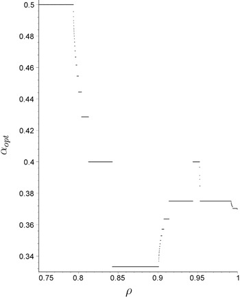
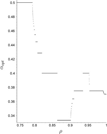
We have used such methods to calculate the optimal polling density d (and thus also the corresponding optimal regular polling policy) for deterministic (λ1,λ2) polling systems where we fix the ratio λ1 /(λ1 + λ2) to be equal to 0.37 by putting λ1 = 0.37ρ and λ2 = 0.73ρ, where the load ρ is varied from zero to one. For this family of polling systems we computed the value of the optimal polling density αopt for both the discrete and the fluid case. For 0 < ρ < 1 we define αopt to be the rational number of lowest denominator that is contained in the nonempty closed subinterval opt(λ1,λ2) of (0,1). We note that in almost all cases for varying (λ1,λ2), the set opt(λ1,λ2) consists of only one (rational) point, which by the above definition is the point αopt. Moreover, in the few cases in which opt(λ1,λ2) consists of more than one point, it still holds by Lemma 4.6.4 in [24] that αopt is unique and thus well defined. In the case ρ = 1 it is easily seen that the interval of stability consists of the single point λ1 /(λ1 + λ2), which is fixed to be 0.37 for this family of polling systems. Thus, it is clear that for ρ = 1 the value of the optimal polling density αopt has to be 0.37 for both the discrete and the fluid cases. For both the discrete and the fluid cases we have computed the value of αopt for varying ρ by implementing Algorithm 3.16 and the appropriate standard techniques for minimizing a convex function in a MAPLE program using exact computations. In Figure 1 the value of αopt is plotted for varying loads for the discrete case, whereas in Figure 2 this is plotted for the fluid case. In both figures the load varies from 0.75 to 1, since it turned out that for smaller loads, the value of αopt is always equal to 0.5, which corresponds to the round-robin polling policy. So, in Figures 1 and 2 we have restricted to an interval with high loads ρ, since this is, by far, the most interesting part of the interval.

The optimal polling density for varying loads for discrete input.

The optimal polling density for varying loads for fluid input.
Remark. We see in Figures 1 and 2 that for this example where λ1 /(λ1 + λ2) = 0.37 the optimal polling density α takes several rational values varying between

and

. We notice that only at the very end of the interval, where ρ = 1, we have that α = 0.37, which is the fraction from the total arriving workload that arrives at queue 1. It is also clearly seen that for low traffic intensity ρ, the optimal ratio α is greater than 0.37, which means that the queue with the smaller arriving workload is served relatively often for small loads. In fact,

, which corresponds to the round-robin policy, is optimal for quite a large part of the interval. We note also that α does not decrease monotonically from

for a small load ρ to 0.37 for ρ = 1. For example, for both the discrete model and the fluid model, there is some part of the interval where

, which is smaller than 0.37. In that case, the queue with the higher workload input is served relatively often. The fact that the optimal polling density

on some part of the interval can be explained from the fact that optimal densities tend to have a low denominator, in general, but that, for example, density

no longer gives a stable policy for such loads. If the load is increased even further, then also

no longer gives a stable policy until, finally, for ρ = 1, we have that only α = 0.37 gives a stable policy.
However, not every change of the optimal α for increasing load is explained by such stability considerations. For example, it is clearly seen in Figures 1 and 2 that

is the optimal polling density on two disjunct intervals of varying loads, whereas for loads between these intervals, we have that α has (among other values) a maximum of

.
Another point of interest that we notice in Figures 1 and 2 is that for any given load, the α for the fluid model is equal or larger than the α for the discrete model. Intuitively this is explained from the fact that for the discrete model, the (whole) packets of workload enter the buffer at once, whereas in the fluid model, it takes more time before the same amount of workload has entered the buffer. So, for the discrete case there should be more urgency to serve the queue where the packets of larger workload arrive. This explains that, for the discrete model, the optimal service rate for the queue with larger input is never lower than for the fluid model and in some cases higher.
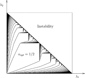
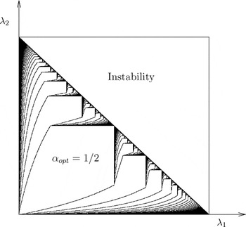
We have also some two-dimensional plots (see Figs. 3 and 4), in which the input rates for the two queues vary independently of each other. To plot Figures 3 and 4 we have calculated the optimal polling density α for various (λ1,λ2) systems in the triangular area {(x1,x2) : x1,x2 ≥ 0,x1 + x2 ≤ 1}. In Figures 3 and 4 there is a black dot at a point (λ1,λ2) within these triangular areas if one or more of the neighboring points has another value of α.

The regions of optimality for discrete input.

The regions of optimality for fluid input.
The resulting Figures 3 and 4 look quite similar to fractal type pictures. It is obvious that both pictures are symmetrical in the diagonal λ1 = λ2. In both figures it is easy to identify the largest (and also most central containing the diagonal λ1 = λ2) white area within the triangle, which corresponds to

. The second largest white areas, which are symmetrically situated with respect to the diagonal λ1 = λ2, correspond to

and

, respectively. We note that these large white areas corresponding to α with a low denominator are somewhat larger in Figure 4 (the fluid model) than in Figure 3 (the discrete model). This supports our conjecture that for the discrete model, the value of

is always greater than or equal to that of the fluid model.
4.3. Structural Results for Deterministic Polling Systems
To obtain more structural results like Proposition 4.2 we restrict ourselves to deterministic polling systems in the sequel of this section. The first result in that case follows from the following properties (which all follow from Section 3) of the function Bλ(d), where λ ∈ [0,1] is the input rate in some queue.
- Bλ(d) = is convex for d ∈ [λ,1]; moreover, Bλ(d) = ∞ for d < λ.
- Bλ(d) is piecewise linear in d and the slope changes only in the best upper approximations of λ, which are rational numbers.
- limε↓0[(Bλ(λ) − Bλ(λ + ε))/ε] = ∞ if λ is irrational.
From these properties the following theorem follows.
Theorem 4.3: Consider a deterministic λ = (λ1,λ2,…, λN) polling system with N ≥ 2 queues such that

. Then there exists some x = (x1,x2,…, xN) ∈ opt(λ) and some j ∈ {1,2,…, N} such that for every i ≠ j, it holds that xi is a best upper approximation of λi.
Corollary 4.4: Let λ = (λ1,λ2,…, λN) be a deterministic polling system with

. Then the set opt(λ) contains a point with rational coordinates.
Remark 4.5: In Section 7 of [14] an algorithm is given to obtain such a rational point for deterministic parallel routing systems. With a slight modification, the same algorithm can be used to find a rational point in the set opt(λ) for deterministic polling systems. Moreover, we note that in most cases the set opt(λ) consists of only one point, which, according to Corollary 4.4 and Theorem 4.3, has rational coordinates and all coordinates except at most one are best upper approximations of the input rate in the corresponding queue.
Combining Theorem 4.2 and Corollary 4.4 it follows that for a deterministic polling system with only two queues and λ1 + λ2 < 1, there exists an optimal regular polling policy with rational densities. It is easily seen that such a policy is periodic. So, we have obtained the following structural result on optimal policies.
Theorem 4.6: For every deterministic (λ1,λ2) polling system with λ1 + λ2 < 1 there exists an optimal regular and periodic polling policy U with B(U) = B*(λ).
We note that a similar result on the optimality of periodic policies for deterministic parallel routing systems with only two queues was obtained in [9]. However, for deterministic λ polling systems with more than two queues we do not have such a result. Indeed, in the case for a rational point (d1,d2,…, dN) ∈ opt(λ), there does not, in general, exist some policy U such that service sequence ui is regular with density di for i = 1,2,…, N. Note that if such a policy U existed, then U would be periodic and also optimal, since B(U) = B*(λ). However, if such a policy does not exist, it is possible that for an optimal policy V, it holds that B(V) > B*(λ). Moreover, such optimal policy V does not necessarily have rational densities (d1,d2,…, dN) ∈ opt(λ) and, thus, it might not be periodic. Nevertheless, we think that in most cases there also exists an optimal periodic policy for deterministic polling systems with more than two queues. Additionally, the following can be proved analogously to the similar result for deterministic parallel routing systems considered in Chapter 5 of [24].
Theorem 4.7: For a deterministic and stable λ polling system with rational input rates λi for i = 1,2,…, N, there exists an optimal routing policy U that is periodic.
Acknowledgment
This work was partially supported by the Van Gogh grant on discrete event systems.
APPENDIX A: On the Optimality of the Bracket Sequence and Its Convexity for the Arrival-Driven Polling Model
Consider an arrival-driven polling model with i.i.d. service and independent i.i.d. interarrival times in every queue. Note that both the deterministic and exponential models that we analyze in this article can be described as such an arrival-driven model with i.i.d. service and independent i.i.d. interarrival times. Moreover, if for queue i in a polling system with these assumptions we have that τ is the mean interarrival time and 1/μi is the mean service time of a job arriving in queue i, then λi, the (expected) workload arriving in queue i per time unit as described in the beginning of Section 4, is given by λi = 1/τμi.
For one queue, Lemma 54 in [2] gives for service sequence a that Vn(a), the expected workload in the queue for the nth arrival starting with an empty queue, is multimodular in a. Since for any service sequence (hence also for the bracket sequence ap(θ)) it holds that

we have that Lemma 1 of [13] can be applied. Hence, the average workload for the bracket sequence with initial phase θ is independent of θ and it is convex in the density p, since

For queue i, let τni denote the nth interarrival time and σni denote the nth service time. Let us further assume that the interarrival (resp. service) time is almost surely bounded from below (resp. above). Hence, almost surely

Then for queues i = 1,2,

and, hence, both satisfy the conditions of Theorem 7 in [2], from which it follows that for queue i = 1,2, the bracket sequence with density pi and any initial phase θi is optimal in the class of policies with upper density smaller than or equal to pi. For service sequences a = (a1,a2) with densities for queue 1 (resp. 2) equal to p1 (resp. p2 = 1 − p1),

The right-hand side (let us denote it with V∞(p1,p2)) is a limit of convex functions and, hence, V∞(p1,p2) is convex in (p1,p2). The proof for unbounded interarrival and service times is similar to the proof of Theorem 22 in [2].
Combining the above results gives the following theorem for an arrival-driven polling model with the i.i.d. and independence assumptions.
Theorem A1: The optimal polling policy for N = 2 queues can be obtained by minimizing the convex function V∞(p1,p2).
APPENDIX B: Computation of the Optimal Policy in the Markovian Case
Here we show how the optimal polling sequence can be computed in a stochastic system consisting of two Poisson arrival queues and one exponential server. As in Appendix A, we consider an arrival-driven polling model with i.i.d. service and independent i.i.d. interarrival times in every queue. We show how the optimal polling between two queues can be computed when the service is exponential (with rate μi in queue i) and the interarrivals are synchronous and exponential (with rate λ in both queues). Other cases can be treated analogously.
We call m(k) the kth polling decision (at arrival k). We set m(k) = 1 if the server is allocated to queue 1 and m(k) = 0 if the server is allocated to queue 2.
We now show that under the polling by a periodic decision word m of period [ell ], the number of customers in a queue can be modeled by a Markov process. The behavior of the number of customers in one queue (say queue 1, and index 1 will be omitted in the following) of the system is given by a continuous-time Markov chain Xt whose state space is equal to

. The first entry represents the number of customers in the queue at time t and the second entry represents the current letter of the polling m (modulo [ell ]).
The continuous-time Markov chain Xt is a quasi-birth-and-death process with generator Q given by

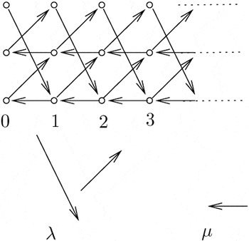
where matrices A0, A1, A2, and C are of size [ell ] × [ell ], with A0 [i,(i + 1) mod [ell ]] = λ, and is null everywhere else, A2 [i,i] = m(i)μ, and is null everywhere else, C[i,i] = −λ, and is null everywhere else, and A1 [i,i] = −λ − m(i)μ and is null everywhere else. An example of the infinitesimal generator Q of Xt when the polling is m = (110)∞ is displayed in Figure B1.

Graph of the infinitesimal generator when the polling is m = (110)∞.
Let π be the invariant measure of the process Xt (when it exists). This probability satisfies

We now refine the notation by introducing block vectors πn of dimension [ell ] whose ith entry (πn(i)) represents the stationary probability to have n customers in the system when the current polling decision is m(i). Hence, πk(1) + ··· + πk([ell ]) is the stationary probability of having k customers in the system. We will not try to compute π directly, which can be quite hard; instead, we will determine its generating function. Let D(0,1) be the closed-unit disk. The generating function of π is the function Π(z) from D(0,1) to

defined by

The following theorem will be used to make sure that the stationary distribution (as well as the function Π(z)) exists.
Lemma B1: The process Xt is positive recurrent if and only if [ell ]λ/aμ < 1.
Proof: This proof is based on Theorem 1.3.2 of [19], which states that Xt is positive recurrent if and only if pA21 > pA01, where 1 is the column vector with all entries equal to one and p is the stationary distribution vector of the finite generator A = A0 + A1 + A2, (i.e., pA = 0 and p1 = 1).
Let us compute p. Using formulas of A0, A1, and A2, we get A = −λI + A0. It should be clear that p1 = p2 = ··· = p[ell ] = 1/[ell ]. Hence, the stability condition becomes pA21 = aμ/[ell ] > pA01 = λ. █
Lemma B2: Let K(z) be the [ell ] × [ell ] matrix defined by

Then the generating function satisfies the functional equation with kernel K(z):

Proof: Using the global balance equation (B1) we get the induction


By multiplying the second equation by zn+1 and by summing, it follows that

which gives Π(z)(z2A0 + zA1 + A2) = π0 μ(1 − z)M, where

█
Let us now study the zeros of K(z). More precisely, we will focus on the zeros inside of the unit disk since Π(z) is a power series with radius of convergence one. Let us call Δ(z) the determinant of the matrix K(z). Using the definition of the matrices A0, A1, and A2, after direct computations one gets

Lemma B3: If [ell ]λ/aμ < 1, then the number of nonnull roots of Δ(z) inside the unit disk is a. Moreover, 0 is a root with multiplicity [ell ] − a.
Proof: It is obvious that 0 is a root with multiplicity [ell ] − a. Let f (z) = (−λz)[ell ]−a(μ − (μ + λ)z)a. Obviously, f has exactly [ell ] roots inside the unit disk.
Now let |z| = 1 + ε. |Δ(z) − f (z)| = λ[ell ](1 + 2[ell ]ε) + o(ε) and | f (z)| ≥ λ[ell ] + (λ[ell ]([ell ] − a) + μa−1(λ + μ)λl−aa)ε + o(ε). A direct computation using the stability condition μ > [ell ]λ/a, shows that |Δ(z) − f (z)| < | f (z)| if ε is small enough. Then, the result follows from Rouché's theorem. █
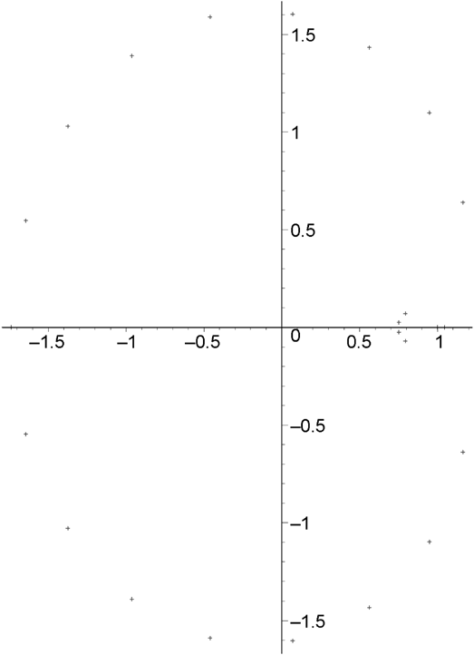
To illustrate the previous lemma, Figure B2 displays all of the roots of Δ(z) when a = 5,[ell ] = 18 and λ = 1,μ = 4. The number of roots inside the unit disk (including 1, which is always a root of Δ(z)) is exactly five.

Roots of Δ(z) when a = 5,[ell ] = 18 and λ = 1,μ = 4.
Theorem B4: If zi is the ith nonnull root of Δ(z) in the unit disk and vi is the right eigenvector of the eigenvalue 0 of K(zi), then π0 is a solution of the system:

where 1 is the column vector with all its components equal to 1.
Proof: If |zi| < 1, then it follows by definition of vi that (1 − zi)μπ0 Mvi = 0. Since zi ≠ 1 and π0(j) = 0 if Mjj = 0, it holds that π0 vi = 0. Note that the rank of the matrix K(zi) is [ell ] − 1; thus, the vector vi is unique up to a multiplicative constant.
The case zi = 1 has to be handled differently since (1 − zi) = 0 and K(1)1 = 0.

since Π(1) = (1/[ell ],…, 1/[ell ]) (easy computation). █
Now we turn back to the two-queue system. Once π0 has been computed, it is possible to compute

and

(j = 1,2), being respectively the expected number of customers and the expected workload in the queue Qj when the polling is made according to m.
Since

, introducing the vector

, which verifies

, yields

In turn, this gives a way to compute the expected workload using the fact that

Now if we consider the system consisting of two synchronous queues, the polling sequence in the second queue is the complementary sequence (m) of the polling in the first one (m). The total workload is

. The optimal polling is a bracket sequence ω(αopt), whose density αopt has to be computed by

Using the fact that this function is convex in the density d (see Appendix A), the optimal density αopt can be computed numerically by gradient descent in a fashion similar to that in [8,10]. We have run several computations using a Maple program implementing the algorithm above (For each triple (λ,μ1,μ2), compute the roots of Δ(z), then compute the corresponding eigenvectors, then compute π0, and, finally, compute the corresponding workload.)
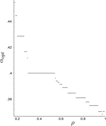
Figure B3 shows the values of αopt, the optimal frequency with which the first queue is served (as in the deterministic case). We have chosen λ = 1 (in both queues) and μ1 /(μ2 + μ1) =

to match the intensities of the deterministic cases. Although one could expect that the stochastic assumption should have a smoothing effect on the value of αopt, the numerical experiments in Figure B3 still suggest that αopt is highly nondifferentiable with many flat zones and many cusps. Moreover, in this case it remains an open problem to (dis)prove the continuity of αopt with respect to varying load ρ.

Computation of the optimal polling ratio αopt when the load ρ varies from 0.2 to 1.
One can also observe that

even when the two queues are not identical, as long as the system is lightly loaded. However, this is only true for very small loads here (ρ < 0.18, to be compared with ρ < 0.78 in the corresponding deterministic case). Finally we note for the heavily loaded system with ρ going to 1 that αopt converges to the ratio of the service intensities, namely 0.37.