1. Introduction
Fluid turbulence is characterized by a wide range of spatial scales, and understanding how energy is distributed and transferred across scales is a fundamental problem. In three-dimensional incompressible turbulence, energy undergoes a cascade from the largest scales of the system, where energy is injected, to the smallest scales, where it is dissipated (Richardson Reference Richardson1922; Tennekes & Lumley Reference Tennekes and Lumley1972; Monin & Yaglom Reference Monin and Yaglom1975; Frisch Reference Frisch1995; Pope Reference Pope2000; Davidson Reference Davidson2015). One of the clearest signatures of the cascade comes from the third-order velocity structure function, which satisfies the Kármán–Howarth equation (Von Kármán & Howarth Reference Von Kármán and Howarth1938). This leads to the celebrated four-fifths law for the third-order structure function (Kolmogorov Reference Kolmogorov1941a , Reference Kolmogorovb ), which indicates energy transfer from large to small scale in the inertial range of turbulence. An alternative approach to quantify energy transfer consists in studying the problem in Fourier space, which leads to the Kármán–Lin equation for the energy spectrum (Lin Reference Lin1947; Von Kármán & Lin Reference Von Kármán and Lin1951), or the subgrid-scale (SGS) stress (Eyink Reference Eyink2006; Ballouz & Ouellette Reference Ballouz and Ouellette2018, Reference Ballouz and Ouellette2020; Dong et al. Reference Dong, Huang, Yuan and Lozano-Durán2020) in the filtered energy equation within the large-eddy simulation (LES) formalism (Germano Reference Germano1992; Meneveau & Katz Reference Meneveau and Katz2000; Sagaut Reference Sagaut2006; Moser, Haering & Yalla Reference Moser, Haering and Yalla2021). Recent attempts have been made to relate the descriptions in Fourier and in real space (Goto, Saito & Kawahara Reference Goto, Saito and Kawahara2017; McKeown et al. Reference McKeown, Pumir, Rubinstein, Brenner and Ostilla-Mónico2023).
Energy transfer is of broader interest than just for incompressible turbulence. Here, we focus on compressible flows, which are of interest not only for fundamental reasons but also for applications to supersonic flows (Kovasznay Reference Kovasznay1953; Spina, Smits & Robinson Reference Spina, Smits and Robinson1994; Modesti et al. Reference Modesti, Sathyanarayana, Salvadore and Bernardini2022), ramjets (Waltrup Reference Waltrup1987; Billig Reference Billig1988; Curran, Heiser & Pratt Reference Curran, Heiser and Pratt1996), volcanic eruptions (Ogden, Glatzmaier & Wohletz Reference Ogden, Glatzmaier and Wohletz2008) and interstellar turbulences (Elmegreen & Scalo Reference Elmegreen and Scalo2004; Scalo & Elmegreen Reference Scalo and Elmegreen2004; Chernyshov, Karelsky & Petrosyan Reference Chernyshov, Karelsky and Petrosyan2010; Ferrand et al. Reference Ferrand, Galtier, Sahraoui and Federrath2020). Numerous studies have investigated the statistics and scaling in compressible turbulence (Samtaney, Pullin & Kosović Reference Samtaney, Pullin and Kosović2001; Pirozzoli & Grasso Reference Pirozzoli and Grasso2004; Wang et al. Reference Wang, Shi, Wang, Xiao, He and Chen2012a , Reference Wang, Shi, Wang, Xiao, He and Chenb , Reference Wang, Gotoh and Watanabe2017; Jagannathan & Donzis Reference Jagannathan and Donzis2016; Donzis & John Reference Donzis and John2020), especially the interscale energy transfer (Bataille & Zhou Reference Bataille and Zhou1999; Aluie Reference Aluie2011; Aluie, Li & Li Reference Aluie, Li and Li2012; Aluie Reference Aluie2013; Eyink & Drivas Reference Eyink and Drivas2018; Schmidt & Grete Reference Schmidt and Grete2019). Conceptually, one may use approaches in terms of structure function (Falkovich, Fouxon & Oz Reference Falkovich, Fouxon and Oz2010; Galtier & Banerjee Reference Galtier and Banerjee2011; Wagner et al. Reference Wagner, Falkovich, Kritsuk and Norman2012; Kritsuk, Wagner & Norman Reference Kritsuk, Wagner and Norman2013; Banerjee & Galtier Reference Banerjee and Galtier2014; Lai, Charonko & Prestridge Reference Lai, Charonko and Prestridge2018; Lindborg Reference Lindborg2019; Hellinger et al. Reference Hellinger, Papini, Verdini, Landi, Franci, Matteini and Montagud-Camps2021a , Reference Hellinger, Verdini, Landi, Papini, Franci and Matteinib ), or focus on the spectral approach (Kida & Orszag Reference Kida and Orszag1992; Miura & Kida Reference Miura and Kida1995).
In general, the introduction of compressibility adds considerable complexity compared with the incompressible case, and it is challenging to extend known theoretical results to compressible turbulence. Difficulties arise as a consequence of varying density, and generally because the velocity gradient tensor is not divergence-free. Generalizations of the Kármán–Howarth equation to compressible flows require density-weighted velocity and velocity structure function (Kida & Orszag Reference Kida and Orszag1992; Falkovich et al. Reference Falkovich, Fouxon and Oz2010; Galtier & Banerjee Reference Galtier and Banerjee2011; Wagner et al. Reference Wagner, Falkovich, Kritsuk and Norman2012; Lai et al. Reference Lai, Charonko and Prestridge2018; Hellinger et al. Reference Hellinger, Verdini, Landi, Papini, Franci and Matteini2021b
), which considerably complicates the mathematical expressions and blurs the physical interpretations of the various terms in the generalized Kármán–Howarth equation. Additionally, the presence of non-zero divergence in the velocity gradient prevents us from obtaining a straightforward relation akin to the four-fifths law observed in incompressible turbulence. These challenges hinder our understanding of how density fluctuations and dilatational motion impact energy transfer in compressible turbulence. Similar difficulties arise when attempting a description in Fourier space. To fully utilize the theoretical findings from incompressible turbulence, a common approach is to decompose the compressible velocity field into solenoidal (divergence-free) and dilatational (compressive) components using Helmholtz decomposition. However, the fluctuation of density complicates this decomposition. Some studies (Fauchet Reference Fauchet1998; Bataille & Zhou Reference Bataille and Zhou1999; Falkovich & Kritsuk Reference Falkovich and Kritsuk2017; Sagaut & Cambon Reference Sagaut and Cambon2018) apply the Helmholtz decomposition directly to the velocity field
 $\boldsymbol{u}$
, resulting in a solenoidal mode with zero divergence, but excluding density variations from the kinetic energy spectrum. Other studies (Kida & Orszag Reference Kida and Orszag1992; Miura & Kida Reference Miura and Kida1995; Wang et al. Reference Wang, Yang, Shi, Xiao, He and Chen2013) decompose the density-weighted velocity field
 $\boldsymbol{w}=\sqrt {\rho }\boldsymbol{u}$
, which takes into account density fluctuations and ensures positive-definiteness, but yields a solenoidal velocity field
 $\boldsymbol{u}^s$
satisfying
 $\boldsymbol{\nabla } \times (\sqrt {\rho }\boldsymbol{u}^s)=0$
, different from the continuity equation of the incompressible fluid
 $\boldsymbol{\nabla } \boldsymbol{\cdot }\boldsymbol{u}^s=0$
, which complicates the physical interpretation of the solenoidal mode.
In this work, we address these technical challenges by applying a filtering approach and extending the formalism recently proposed by Johnson (Reference Johnson2020, Reference Johnson2021) to compressible turbulence, and unveil the physical mechanism associated with dilatational motion. Johnson (Reference Johnson2020) previously showed that the SGS stress can be expressed as an integral of the filtered velocity gradient across all subfilter scales. This approach identifies three mechanisms contributing to energy flux: strain self-amplification; vortex stretching; and mixed strain–vorticity interaction. By conducting direct numerical simulations (DNSs), Johnson (Reference Johnson2020) revealed that strain self-amplification dominates the energy cascade process. This formalism has also been extended to sheared, stably stratified turbulence (Zhang et al. Reference Zhang, Dhariwal, Portwood, Kops and Bragg2022) and helical turbulence (Capocci et al. Reference Capocci, Johnson, Oughton, Biferale and Linkmann2023). Here, we show that when applied to compressible turbulence, this approach helps identify how dilatational motion contributes to the energy flux.
In § 2, we will first generalize the relation between SGS stress and filtered velocity gradient for incompressible turbulence with a Gaussian filter, introduced by Johnson (Reference Johnson2020; Reference Johnson2021), to the case of compressible turbulence using the Favre filtering, and introduce new mechanisms associated with dilatational motion. Then, in §§ 3 and 4, we will use DNS data to verify our theoretical derivation and analyse the dilatational contribution to energy transfer. Finally, in § 5, we summarize the results of this work.
2. Relation between SGS stress and filtered velocity gradient in compressible turbulence
We first start from the SGS stress term in compressible turbulence,
 \begin{equation} \tau _{\textit{ij}}^\ell = \overline {\rho }^\ell \widetilde {u_i u_j}^\ell - \overline {\rho }^{\ell}\widetilde {u}_i^\ell \widetilde {u}_j^\ell = \overline {\rho u_i u_j}^\ell - \frac {1}{\overline {\rho }^\ell } \overline {\rho u_i}^\ell \overline {\rho u_j}^\ell , \end{equation}
where the symbols
 $\overline {\boldsymbol{\cdot }}^\ell$
and
 $\widetilde {\phi }^\ell = \overline {\rho \phi }^\ell /\overline {\rho }^\ell$
denote the spatial and Favre filtering at scale
 $\ell$
, see, e.g. Chai & Mahesh (Reference Chai and Mahesh2012) and Qi et al. (Reference Qi, Li, Hu and Yu2022). If we choose the spatial filter to be Gaussian, then we have the following identity (Johnson Reference Johnson2020; Reference Johnson2021):
 \begin{equation} \frac {\partial \overline {\phi }^\ell }{\partial \ell ^2} = \frac {1}{2}{\nabla} ^2 \overline {\phi }^\ell . \end{equation}
To address the effect of density fluctuation, we need to evaluate derivatives related to Favre filtering. We first look at
 ${(\partial \widetilde {\phi }^\ell)}/{(\partial \ell ^2)}$
,
 \begin{align} \frac {\partial \widetilde {\phi }^\ell }{\partial \ell ^2} &= \frac {\partial }{\partial \ell ^2} \left (\frac {\overline {\rho \phi }^\ell }{\overline {\rho }^\ell }\right ) = \frac {1}{2}\left [ \frac {1}{\overline {\rho }^\ell } {\nabla} ^2 (\overline {\rho \phi }^\ell ) - \frac {\overline {\rho \phi }^\ell }{(\overline {\rho }^\ell )^2} {\nabla} ^2 (\overline {\rho }^\ell ) \right ]\!. \end{align}
Next, we consider
 ${\nabla} ^2 \widetilde {\phi }^\ell$
,
 \begin{align} {\nabla} ^2 \widetilde {\phi }^\ell & = {\nabla} ^2 \left ( \frac {\overline {\rho \phi }^\ell }{\overline {\rho }^\ell } \right ) \nonumber \\ & = \frac {1}{\overline {\rho }^\ell } {\nabla} ^2 (\overline {\rho \phi }^\ell ) - \frac {2}{(\overline {\rho }^\ell )^2} \frac {\partial \overline {\rho }^\ell }{\partial x_k} \frac {\partial \overline {\rho \phi }^\ell }{\partial x_k} + \frac {2\overline {\rho \phi }^\ell }{(\overline {\rho }^\ell )^3} \frac {\partial \overline {\rho }^\ell }{\partial x_k} \frac {\partial \overline {\rho }^\ell }{\partial x_k} -\frac {\overline {\rho \phi }^\ell }{(\overline {\rho }^\ell )^2} {\nabla} ^2 (\overline {\rho }^\ell ). \end{align}
Subtracting one-half of (2.4) from (2.3) yields
 \begin{align} \frac {\partial \widetilde {\phi }^\ell }{\partial \ell ^2} - \frac {1}{2} {\nabla} ^2 \widetilde {\phi }^\ell = \frac {1}{(\overline {\rho }^\ell )^2} \frac {\partial \overline {\rho }^\ell }{\partial x_k} \frac {\partial \overline {\rho \phi }^\ell }{\partial x_k} - \frac {\overline {\rho \phi }^\ell }{(\overline {\rho }^\ell )^3} \frac {\partial \overline {\rho }^\ell }{\partial x_k} \frac {\partial \overline {\rho }^\ell }{\partial x_k} = \frac {1}{\overline {\rho }^\ell } \frac {\partial \overline {\rho }^\ell }{\partial x_k} \frac {\partial \widetilde {\phi }^\ell }{\partial x_k}. \end{align}
Now with the help of (2.5), we evaluate
 ${\partial \tau _{\textit{ij}}^\ell }/{\partial \ell ^2}$
,
 \begin{align} \frac {\partial \tau _{\textit{ij}}^\ell }{\partial \ell ^2} &= \frac {\partial \overline {\rho }^\ell }{\partial \ell ^2} \widetilde {u_i u_j}^\ell + \overline {\rho }^\ell \frac {\partial \widetilde {u_i u_j}^\ell }{\partial \ell ^2} - \frac {\partial \overline {\rho }^{\ell}}{\partial \ell ^2} \widetilde {u}_i^\ell \widetilde {u}_j^\ell - \overline {\rho }^{\ell} \frac {\partial \widetilde {u}_i^\ell }{\partial \ell ^2} \widetilde {u}_j^\ell - \overline {\rho }^{\ell} \widetilde {u}_i^\ell \frac {\partial \widetilde {u}_j^\ell }{\partial \ell ^2} \notag \\&= \left [\frac {1}{2} {\nabla} ^2 (\overline {\rho }^\ell ) \widetilde {u_i u_j}^\ell \right ] + \left [\frac {1}{2} \overline {\rho }^\ell {\nabla} ^2 \widetilde {u_i u_j}^\ell + \frac {\partial \overline {\rho }^\ell }{\partial x_k}\frac {\partial \widetilde {u_i u_j}^\ell }{\partial x_k}\right ] - \left [\frac {1}{2} {\nabla} ^2 (\overline {\rho }^\ell ) \widetilde {u_i}^\ell \widetilde {u_j}^\ell \right ] \notag \\ &\quad - \left [\frac {1}{2}\overline {\rho }^\ell {\nabla} ^2 (\widetilde {u_i}^\ell ) \widetilde {u_j}^\ell + \frac {\partial \overline {\rho }^\ell }{\partial x_k}\frac {\partial \widetilde {u_i}^\ell }{\partial x_k} \widetilde {u_j}^\ell \right ] - \left [\frac {1}{2}\overline {\rho }^\ell {\nabla} ^2 (\widetilde {u_j}^\ell ) \widetilde {u_i}^\ell + \frac {\partial \overline {\rho }^\ell }{\partial x_k}\frac {\partial \widetilde {u_j}^\ell }{\partial x_k} \widetilde {u_i}^\ell \right ]\!. \end{align}
On the other hand, we also have
 \begin{align} \frac {1}{2} {\nabla} ^2 \tau _{\textit{ij}}^\ell &= \frac {1}{2}\frac {\partial }{\partial x_k} \left (\frac {\partial \overline {\rho }^\ell }{\partial x_k} \widetilde {u_i u_j}^\ell + \overline {\rho }^\ell \frac {\partial \widetilde {u_i u_j}^\ell }{\partial x_k} - \frac {\partial \overline {\rho }^{\ell}}{\partial x_k} \widetilde {u}_i^\ell \widetilde {u}_j^\ell - \overline {\rho }^{\ell} \frac {\partial \widetilde {u}_i^\ell }{\partial x_k} \widetilde {u}_j^\ell - \overline {\rho }^{\ell} \widetilde {u}_i^\ell \frac {\partial \widetilde {u}_j^\ell }{\partial x_k} \right ) \notag \\ &= \frac {1}{2} {\nabla} ^2 (\overline {\rho }^\ell ) \widetilde {u_i u_j}^\ell + \frac {1}{2} \overline {\rho }^\ell {\nabla} ^2 \widetilde {u_i u_j}^\ell + \frac {\partial \overline {\rho }^\ell }{\partial x_k}\frac {\partial \widetilde {u_i u_j}^\ell }{\partial x_k} - \frac {1}{2} {\nabla} ^2 (\overline {\rho }^\ell ) \widetilde {u_i}^\ell \widetilde {u_j}^\ell \notag \\ &\quad - \frac {\partial \overline {\rho }^\ell }{\partial x_k}\frac {\partial \widetilde {u_i}^\ell }{\partial x_k} \widetilde {u_j}^\ell - \frac {\partial \overline {\rho }^\ell }{\partial x_k}\frac {\partial \widetilde {u_j}^\ell }{\partial x_k} \widetilde {u_i}^\ell - \overline {\rho }^\ell \frac {\partial \widetilde {u_i}^\ell }{\partial x_k}\frac {\partial \widetilde {u_j}^\ell }{\partial x_k} - \frac {1}{2}\overline {\rho }^\ell {\nabla} ^2 (\widetilde {u_i}^\ell ) \widetilde {u_j}^\ell \notag \\ &\quad - \frac {1}{2}\overline {\rho }^\ell {\nabla} ^2 (\widetilde {u_j}^\ell ) \widetilde {u_i}^\ell . \end{align}
Subtracting (2.7) from (2.6) yields
 \begin{equation} \frac {\partial \tau _{\textit{ij}}^\ell }{\partial \ell ^2} = \frac {1}{2} {\nabla} ^2 \tau _{\textit{ij}}^\ell + \overline {\rho }^\ell \frac {\partial \widetilde {u_i}^\ell }{\partial x_k}\frac {\partial \widetilde {u_j}^\ell }{\partial x_k}. \end{equation}
The solution of (2.8) is
 \begin{align} \tau _{\textit{ij}}^\ell &= \int _0^{\ell ^2} \overline {\overline {\rho }^{\sqrt \alpha } \frac {\partial \widetilde {u_i}^{\sqrt \alpha }}{\partial x_k}\frac {\partial \widetilde {u_j}^{\sqrt \alpha }}{\partial x_k}}^{\sqrt {\ell ^2 - \alpha }} \textrm {d}\alpha \notag \\ &= \int _0^{\ell ^2} \overline {\overline {\rho }^{\sqrt \alpha } \widetilde {A}_{\textit{ik}}^{\sqrt \alpha } \widetilde {A}_{\textit{jk}}^{\sqrt \alpha } }^{\sqrt {\ell ^2 - \alpha }}\textrm {d}\alpha , \end{align}
where
 $\widetilde {A}_{\textit{ij}}^{\ell } \equiv \partial \widetilde {u_i}^{\ell }/\partial x_j$
is the gradient of the Favre-filtered velocity, referred to in the following as filtered velocity gradient. Its divergence-free, symmetric and antisymmetric parts are defined by
 $\widetilde {S}_{\textit{ij}}^{\ell } = ( \widetilde {A}_{\textit{ij}}^{\ell } + \widetilde {A}_{\textit{ji}}^{\ell } )/2 -\widetilde {A}_{\textit{ll}}^{\ell } \delta _{\textit{ij}}/3$
and
 $\widetilde {W}_{\textit{ij}}^{\ell } = ( \widetilde {A}_{\textit{ij}}^{\ell } - \widetilde {A}_{\textit{ji}}^{\ell } )/2$
, respectively. Note that (2.9) in our text and equation (10) in Johnson (Reference Johnson2020) share a similar form, the differences being that a factor of density appears, and the substitution of standard filtering with Favre filtering for the filtered velocity gradient in the compressible case considered here.
The quantity
 $\varPi ^\ell \equiv \tau _{\textit{ij}}^\ell ({\partial \widetilde {u_i}^{\ell }}/{\partial x_j})$
represents the energy transfer across length scale
 $\ell$
, with
 $\varPi ^\ell \lt 0$
indicating an energy flux from scales larger than
 $\ell$
to scales smaller than
 $\ell$
. By substituting the velocity gradient decomposition
 $\widetilde {A}_{\textit{ij}} = \widetilde {S}_{\textit{ij}}+\widetilde {W}_{\textit{ij}}+\widetilde {A}_{\textit{ll}}\delta _{\textit{ij}}/3$
into (2.9), the interscale energy transfer term
 $\varPi ^{\ell }$
decomposes as follows:
 \begin{align} \varPi ^{\ell } =\underbrace {\varPi ^{\ell }_{s1} + \varPi ^{\ell }_{s2} + \varPi ^{\ell }_{s3}}_{\varPi ^{\ell }_s} + \underbrace {\varPi ^{\ell }_{m1} + \varPi ^{\ell }_{m2} + \varPi ^{\ell }_{m3}}_{\varPi ^{\ell }_m} + \varPi ^{\ell }_d, \end{align}
where
 \begin{align}\varPi ^{\ell }_{s1} &= \int _0^{\ell ^2} \textrm {d}\alpha \overline {\overline {\rho }^{\sqrt \alpha } \widetilde {S}_{\textit{ik}}^{\sqrt \alpha } \widetilde {S}_{\textit{jk}}^{\sqrt \alpha } }^{\sqrt {\ell ^2 - \alpha }} \widetilde {S}_{\textit{ij}}^{\ell }, \end{align}
 \begin{align}\varPi ^{\ell }_{s2} &= - \int _0^{\ell ^2} \textrm {d}\alpha \overline {\overline {\rho }^{\sqrt \alpha } \widetilde {W}_{\textit{ik}}^{\sqrt \alpha } \widetilde {W}_{\textit{kj}}^{\sqrt \alpha } }^{\sqrt {\ell ^2 - \alpha }} \widetilde {S}_{\textit{ij}}^{\ell }, \end{align}
 \begin{align}\varPi ^{\ell }_{s3} &= \int _0^{\ell ^2} \textrm {d}\alpha \overline {\overline {\rho }^{\sqrt \alpha } \left (\widetilde {S}_{\textit{kj}}^{\sqrt \alpha } \widetilde {W}_{\textit{ik}}^{\sqrt \alpha } - \widetilde {S}_{\textit{ik}}^{\sqrt \alpha } \widetilde {W}_{\textit{kj}}^{\sqrt \alpha }\right )}^{\sqrt {\ell ^2 - \alpha }} \widetilde {S}_{\textit{ij}}^{\ell }, \end{align}
 \begin{align}\varPi ^{\ell }_{m1} &= \frac {2}{3} \int _0^{\ell ^2} \textrm {d}\alpha \overline {\overline {\rho }^{\sqrt \alpha } \widetilde {A}_{\textit{ll}}^{\sqrt \alpha } \widetilde {S}_{\textit{ij}}^{\sqrt \alpha } }^{\sqrt {\ell ^2 - \alpha }} \widetilde {S}_{\textit{ij}}^{\ell }, \end{align}
 \begin{align}\varPi ^{\ell }_{m2} &= \frac {1}{3}\int _0^{\ell ^2} \textrm {d}\alpha \overline {\overline {\rho }^{\sqrt \alpha } \widetilde {S}_{\textit{ij}}^{\sqrt \alpha } \widetilde {S}_{\textit{ij}}^{\sqrt \alpha } }^{\sqrt {\ell ^2 - \alpha }} \widetilde {A}_{\textit{ll}}^{\ell }, \end{align}
 \begin{align}\varPi ^{\ell }_{m3} &= - \frac {1}{3}\int _0^{\ell ^2} \textrm {d}\alpha \overline {\overline {\rho }^{\sqrt \alpha } \widetilde {W}_{\textit{ij}}^{\sqrt \alpha } \widetilde {W}_{\textit{ji}}^{\sqrt \alpha } }^{\sqrt {\ell ^2 - \alpha }} \widetilde {A}_{\textit{ll}}^{\ell }, \end{align}
 \begin{align}\varPi ^{\ell }_d &= \frac {1}{9}\int _0^{\ell ^2} \textrm {d}\alpha \overline {\overline {\rho }^{\sqrt \alpha } \widetilde {A}_{\textit{ii}}^{\sqrt \alpha } \widetilde {A}_{\textit{jj}}^{\sqrt \alpha } }^{\sqrt {\ell ^2 - \alpha }} \widetilde {A}_{\textit{kk}}^{\ell } . \end{align}
In (2.10), the interscale energy transfer is decomposed into three parts:
 $\varPi ^{\ell }_s$
, the energy transfer solely due to the solenoidal motion (hereafter referred to as solenoidal energy transfer);
 $\varPi ^\ell _m$
, the energy transfer resulting from the interaction between solenoidal and dilatational motions (hereafter referred to as mixed energy transfer); and
 $\varPi ^\ell _{d}$
, the energy transfer solely due to the dilatational motion (hereafter referred to as dilatational energy transfer). More precisely, the solenoidal energy transfer has three contributions:
 $\varPi ^{\ell }_{s1}$
,
 $\varPi ^{\ell }_{s2}$
and
 $\varPi ^{\ell }_{s3}$
, which represent the energy transfer due to the interaction of strain at scale
 $\ell$
with strain (see (2.11a
)), vorticity (see (2.11b
)) and strain–vorticity correlations (see (2.11c
)) at a scale smaller than or equal to
 $\ell$
, respectively. These terms correspond to
 $\varPi ^{\ell }_{S}$
,
 $\varPi ^{\ell }_{\varOmega }$
and
 $\varPi ^{\ell }_{c}$
introduced in the incompressible case by Johnson (Reference Johnson2020) and Yang et al. (Reference Yang, Zhou, Xu and He2023). The mixed energy transfer
 $\varPi ^{\ell }_{m}$
is also composed of three terms:
 $\varPi ^{\ell }_{m1}$
,
 $\varPi ^{\ell }_{m2}$
and
 $ \varPi ^{\ell }_{m3}$
. The first one,
 $\varPi ^{\ell }_{m1}$
, see (2.11d
), represents the energy transfer resulting from the interaction between strain at scale
 $\ell$
and the strain–dilatation correlation at a scale smaller than or equal to
 $\ell$
. The terms
 $\varPi ^{\ell }_{m2}$
(see (2.11e
)), respectively,
 $\varPi ^{\ell }_{m3}$
(see (2.11f
)) describe the energy transfer resulting from the interaction between dilatation at scale
 $\ell$
and strain, respectively, vorticity. Finally, the dilatational energy transfer
 $\varPi ^{\ell }_{d}$
(see (2.11g
)) arises from the interaction between dilatation at scale
 $\ell$
and dilatation at a scale smaller than or equal to
 $\ell$
.
Furthermore, (2.9) can be decomposed into scale-local (
 $l$
) and scale non-local (
 $nl$
) parts, i.e.
 \begin{equation} \tau _{\textit{ij}}^\ell = \ell ^2 \overline {\rho }^\ell \widetilde {A}_{\textit{ik}}^{\ell } \widetilde {A}_{\textit{jk}}^{\ell } + \!\int _{0}^{\ell ^2} \!\textrm {d}\alpha \!\left ( \overline {\overline {\rho }^{\sqrt \alpha } \widetilde {A}_{\textit{ik}}^{\sqrt \alpha } \widetilde {A}_{\textit{jk}}^{\sqrt \alpha } }^{\sqrt {\ell ^2 - \alpha }} - \overline {\overline {\rho }^{\sqrt \alpha }}^{\sqrt {\ell ^2 - \alpha }} \overline {\widetilde {A}_{\textit{ik}}^{\sqrt \alpha }}^{\sqrt {\ell ^2 - \alpha }} \overline {\widetilde {A}_{\textit{jk}}^{\sqrt \alpha }}^{\sqrt {\ell ^2 - \alpha }} \right )\!. \end{equation}
The scale-local contributions involve only quantities defined at scale
 $\ell$
, while the scale non-local contributions involve velocity gradients at scales finer than
 $\ell$
. Then we can decompose the interscale energy transfer terms as a sum of a scale-local and scale non-local contributions, i.e.
 \begin{equation} \varPi ^{\ell }_{x} = \varPi ^{\ell }_{x,l} + \varPi ^{\ell }_{x,nl}, \end{equation}
where
 $x$
denotes one of the subscripts
 $s1$
,
 $s2$
,
 $s3$
,
 $m1$
,
 $m2$
,
 $m3$
or
 $d$
. We find that
 $\varPi ^{\ell }_{s3,l}=0$
, the other local contributions being expressible in terms of the five independent components of the third-order velocity gradient moment discussed in Yang et al. (Reference Yang, Fang, Fang, Pumir and Xu2022),
 \begin{align}\varPi ^{\ell }_{s1,l} &= \overline {\rho }^{\ell } \widetilde {S}_{\textit{ik}}^{\ell } \widetilde {S}_{\textit{jk}}^{\ell } \widetilde {S}_{\textit{ij}}^{\ell } \ell ^2,\\[-13pt]\nonumber\end{align}
 \begin{align}\varPi ^{\ell }_{s2,l} &= - \overline {\rho }^{\ell } \widetilde {W}_{\textit{ik}}^{\ell } \widetilde {W}_{\textit{kj}}^{\ell }\widetilde {S}_{\textit{ij}}^{\ell } \ell ^2,\\[-13pt]\nonumber\end{align}
 \begin{align}\varPi ^{\ell }_{m1,l} &= 2\varPi ^{\ell }_{m2,l} = \frac {2}{3}\overline {\rho }^{\ell } \widetilde {S}_{\textit{ij}}^{\ell } \widetilde {S}_{\textit{ij}}^{\ell } \widetilde {A}_{\textit{ll}}^{\ell } \ell ^2,\\[-13pt]\nonumber\end{align}
 \begin{align}\varPi ^{\ell }_{m3,l} &= - \frac {1}{3} \overline {\rho }^{\ell } \widetilde {W}_{\textit{ij}}^{\ell } \widetilde {W}_{\textit{ji}}^{\ell } \widetilde {A}_{\textit{ll}}^{\ell } \ell ^2, \end{align}
 \begin{align}\varPi ^{\ell }_{d,l} &= \frac {1}{9}\overline {\rho }^{\ell } \widetilde {A}_{\textit{ii}}^{\ell } \widetilde {A}_{\textit{jj}}^{\ell } \widetilde {A}_{\textit{kk}}^{\ell } \ell ^2. \end{align}
The scale non-local contributions corresponding to the various local terms in (2.14) can also be expressed analogously to the one in (2.12).
3. Numerical methods and case configurations
To analyse the dilatational contribution of compressible turbulence using the approach developed above, we use DNS of freely decaying and forced compressible homogeneous isotropic turbulence. To this end, we first solved numerically the compressible Navier–Stokes equations. In this section, we briefly introduce the governing equation, the numerical set-up and the computational fluid dynamics solver. We also provide elementary information about the simulated flows.
For the non-dimensional Navier–Stokes equations, we select the reference quantities
 $\rho _0$
for density,
 $L_0$
for length,
 $T_0$
for temperature,
 $u_0$
for velocity and
 $\mu _0$
for viscosity. These five reference quantities are grouped into two dimensionless numbers: the Reynolds number
 $\textit{Re}=\rho _0 u_0 L_0/\mu _0$
, which quantifies the scale separation of the flow, and the Mach number
 ${Ma}=u_0/\sqrt {\gamma R T_0}$
that measures the compressibility of the fluid. Here
 $R$
is the specific gas constant and
 $\gamma =1.4$
is the ratio of specific heats. These two dimensionless numbers are set at the start of each run and remain constant throughout the simulation. The non-dimensional compressible Navier–Stokes equations are expressed as
 \begin{align}\frac {\partial \rho }{\partial t} + \frac {\partial \rho u_i}{\partial x_i} &= 0, \end{align}
 \begin{align}\frac {\partial \rho u_i}{\partial t} + \frac {\partial }{\partial x_j}\left (\rho u_i u_j + p\delta _{\textit{ij}}\right ) - \frac {\partial \sigma _{\textit{ij}}}{\partial x_j} - f_i &= 0, \end{align}
 \begin{align}\frac {\partial \mathcal{E}}{\partial t} + \frac {\partial }{\partial x_j}\left [\left (\mathcal{E}+p\right )u_j\right ] - \frac {\partial }{\partial x_j}\left (\sigma _{\textit{ij}}u_i - Q_j\right ) - f_i u_i + \kappa T^4 &= 0, \end{align}
in which
 $p=\rho T/(\gamma \textit{Ma}^{2})$
is the pressure,
 $\sigma _{\textit{ij}}=\mu [(\partial u_i/\partial x_j)+(\partial u_j/\partial x_i)- ({2}/{3})(\partial u_k/\partial x_k)\delta _{\textit{ij}}]$
is the non-dimensional viscous stress tensor with the effect of bulk viscosity neglected (Pan & Johnsen Reference Pan and Johnsen2017),
 $\mathcal{E}= ({1}/{2}) \rho u_i u_i + p/(\gamma -1)$
is the dimensionless total energy and
 $Q_j= - \mu /[\textit{Pr}\times\textit{Re}(\gamma -1) \times\textit{Ma}^{2}] \times(\partial T/\partial x_j)$
is the dimensionless heat flux with a constant Prandtl number
 $\textit{Pr}=0.72$
. The terms
 $-f_i$
in (3.1b
) and
 $-f_i u_i + \kappa T^4$
in (3.1c
) represent the external forcing and radiation mechanisms in the compressible flow field. These terms will be elaborated upon for each specific type of run. The viscosity follows Sutherland’s law (William Reference William1893) with
 $\mu =T^{3/2} (T_0+T_{\textit{ref}})/ [(T T_0+T_{\textit{ref}}) \textit{Re} ]$
.
Equations (3.1a )–(3.1c ) are solved with a high-order finite difference method. Specifically, the convective terms are calculated by a seventh-order low-dissipative monotonicity-preserving scheme (Fang, Li & Lu Reference Fang, Li and Lu2013) such that shockwaves in a compressible flow can be captured and the capabilities of resolving small-scale turbulent structures are preserved. The diffusion terms are discretized by a sixth-order compact central scheme (Lele Reference Lele1992) with a domain decoupling scheme for parallel computation (Fang et al. Reference Fang, Gao, Moulinec and Emerson2019). The time integration is computed by a three-step third-order total variation diminishing Runge–Kutta method (Gottlieb & Shu Reference Gottlieb and Shu1998). For the flow simulations in this study, we utilize the open-source solver ASTR, which has been extensively validated in DNSs of various compressible turbulent flows with and without shockwaves (Fang et al. Reference Fang, Li and Lu2013, Reference Fang, Yao, Li and Lu2014, Reference Fang, Yao, Zheltovodov, Li and Lu2015, Reference Fang, Zhang, Fang and Zhu2016, Reference Fang, Zheltovodov, Yao, Moulinec and Emerson2020; Yang et al. Reference Yang, Fang, Fang, Pumir and Xu2022).
For all freely decaying and forced runs, the computational domain for our numerical simulations is a
 $(2\pi )^3$
cube with periodic conditions in all three directions, discretized with a
 $512^3$
mesh. In our study, the statistical quantities of the flow are defined as follows. The Taylor microscale Reynolds number is defined as
 $R_\lambda = \left \langle \rho \right \rangle u' \lambda / (\sqrt {3}\left \langle \mu \right \rangle )$
, where
 $u' = \sqrt {\left \langle u_i u_i \right \rangle }$
is the root-mean-square velocity and
 $\lambda = u' / (\sum_i \langle ( \partial u_i/\partial x_i)^2 \rangle /3)^{1/2}$
is the Taylor microscale, where
 $\langle \boldsymbol{\cdot }\rangle$
denotes the average over space. The turbulent Mach number is given by
 $\textit{Ma}_t = {Ma} {\times}u' / \langle \sqrt {\gamma R T} \rangle$
. The Kolmogorov scale is defined as
 $\eta = (\left \langle \mu / \rho \right \rangle ^3 / \varepsilon )^{1/4}$
, where the energy dissipation rate is
 $\varepsilon = \langle \sigma _{\textit{ij}} \mathring{S}_{\textit{ij}} / \rho \rangle$
and
 $\mathring S_{\textit{ij}} = (\partial u_i /\partial x_j +\partial u_j / \partial x_i)/2$
. The integral length scale is defined as
 $L = u'^3 / (\varepsilon / \left \langle \rho \right \rangle )$
. Since the mean velocity
 $\left \langle u_i \right \rangle$
is zero for all runs, the turbulent kinetic energy is defined as
 $\mathcal{K} = \left \langle \rho u_i u_i \right \rangle / 2$
. The skewness is defined as
 $\mathcal{S} = ( \sum _i \langle (\partial u_i/\partial x_i)^3 \rangle ) / (\sum _i \langle (\partial u_i/\partial x_i)^2 \rangle ^{3/2} )$
. Additionally, we performed a forced run at a higher resolution
 $(1024^3)$
, at a Reynolds number
 $R_\lambda = 240$
, and
 $\textit{Ma}_t = 1.1$
. The results (not shown) clearly demonstrate that the results shown in the paper are not an artefact of the moderate Reynolds number used in the manuscript.
3.1. Configuration and statistics of freely decaying runs
For the freely decaying runs, the initial velocity field is divergence-free, with an energy spectrum
 $E(k)=Ak^4 \exp (-2k^2/k_0^2)$
,
 $k_0=4$
being the wavenumber where the energy spectrum peaks and
 $A$
determining the initial energy. The density,
 $\rho$
, pressure,
 $p$
, and temperature,
 $T$
, are all initialized as constant, following the ‘IC4’ configuration of Samtaney et al. (Reference Samtaney, Pullin and Kosović2001). The external force
 $f_i$
and the radiation coefficient
 $\kappa$
are set as zero. We simulated in total four flows, with different initial turbulent Mach numbers:
 $\textit{Ma}_t=1.00$
,
 $0.65$
,
 $0.32$
,
 $0.10$
(referred to as 1D, 2D, 3D and 4D, respectively; ‘D’ represents freely decaying). The initial Taylor-scale Reynolds number is set as
 $R_\lambda =626.21$
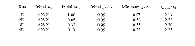
for all runs. The main parameters characterizing the simulations are summarized in table 1. Although simulated with a compressible Navier–Stokes solver, the flow 4D can effectively be considered as incompressible, given that their Mach numbers are extremely small. In the following, we use the initial large-eddy-turnover time
 $\tau _0 = (\int _{0}^{\infty }E(k)/k \textrm {d} k )/u'^3$
to normalize time in the simulations of these runs.
Numerical setting and basic statistics of freely decaying runs.

Evolution of global statistics of freely decaying runs. Red circle, blue square, magenta diamond and orange triangle lines refer to runs 1D, 2D, 3D and 4D, respectively. (a) The turbulent kinetic energy
 $\mathcal{K}$
normalized by its initial value
 $\mathcal{K}_0$
and the Kolmogorov scale
 $\eta$
divided by the grid length
 $\Delta x = 2\pi /512$
(shown in the inset), the horizontal dashed line marks
 $0.5$
. (b) The Reynolds number based on the Taylor microscale
 $R_\lambda$
. (c) The turbulent Mach number
 $\textit{Ma}_t$
. (d) The velocity gradient skewness
 $\mathcal{S}$
.

Figure 1 illustrates the evolution of global statistics for the freely decaying runs. As shown in figure 1(a), the Kolmogorov scale first decreases due to the development of strong compression. After reaching its minimum at time
 $t_{\eta ,\textit{min} {}}$
, the Kolmogorov scale
 $\eta$
subsequently increases as the flow transitions into a decaying regime. After
 $t_{\eta ,\textit{min} {}}$
, figure 1(a–c) shows that the turbulent kinetic energy
 $\mathcal{K}$
, the Taylor-scale Reynolds number
 $R_\lambda$
, and the turbulent Mach number
 $\textit{Ma}_t$
all decay monotonically. Thus,
 $t_{\eta ,\textit{min} {}}$
can be regarded as the starting time of the decay. The initial Kolmogorov scale, the minimum Kolmogorov scale and the time of the minimal Kolmogorov scale
 $t_{\eta ,\textit{min} {}}$
are presented in table 1,
 $\Delta x$
being the grid spacing. For all runs,
 $\eta /\Delta x$
remains above
 $0.5$
, ensuring adequate resolution according to classical criteria of
 $\eta /\Delta x\geqslant 0.5$
(Petersen & Livescu Reference Petersen and Livescu2010; Wang et al. Reference Wang, Shi, Wang, Xiao, He and Chen2012a
). We also found that, during the decay, the integral scale
 $L$
remains less than one-third of the size of the computational domain (not shown), ensuring that the largest turbulent structures are adequately contained within the simulation box.
Figure 1(a,b) shows that the turbulent kinetic energy
 $\mathcal{K}$
and the Taylor-scale Reynolds number
 $R_\lambda$
all decay monotonically with time. Furthermore, while the curves of
 $\mathcal{K}$
and
 $R_\lambda$
deviate from each other during the initial stages, the curves collapse at later time during the decay. This observation suggests that, over the range considered here, compressibility does not significantly impact global dissipation during the decay stage. Nevertheless, in runs 1D, 2D, 3D, despite the relatively low turbulent Mach number towards the end of the simulation, compressible effects persist in the flow field with the presence of spatially distributed shocklets in the flow. In comparison, in our simulations 4D, the flow remains incompressible throughout the calculation. The skewness of velocity gradient
 $\mathcal{S}$
, shown in figure 1(d), exhibits a sharp negative peak for runs 1D and 2D at approximately
 $t/\tau _0 \approx 0.35$
, reflecting the transient from the initial divergence-free velocity field to a compressible flow field. In contrast, for runs 3D and 4D, the skewness decreases during the initial stage. Once the turbulent regime is well established, the skewness remains nearly constant at approximately
 $- \mathcal{S} \approx 0.5$
, which agrees with the theoretical estimates for incompressible turbulence as described in Qian (Reference Qian1994), reflecting that all our runs are weakly compressible. Overall, our results are consistent with the scaling proposed by Donzis & John (Reference Donzis and John2020).
In our analysis in § 4, we will focus mostly on the flow field at a single moment in the decaying regime, namely
 $t/\tau _0 = 5.59$
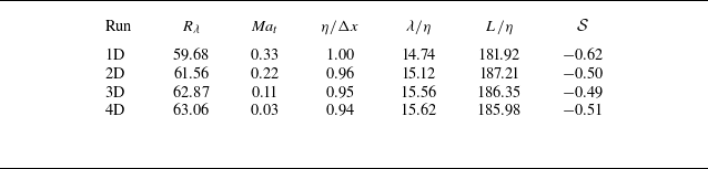
. Table 2 lists some of the essential global statistical quantities at the selected time. As the flow is homogenous but not steady, the ensemble average quantities are only represented by the spatial average of corresponding quantities at all
 $512^3$
points. Note that at this moment, the turbulent Mach numbers
 $\textit{Ma}_t$
in all runs satisfy
 $\textit{Ma}_t \lesssim 0.3$
and correspond to the low-
 $\textit{Ma}_t$
regime (Jagannathan & Donzis Reference Jagannathan and Donzis2016).
Global statistics of freely decaying runs at the moment
 $t/\tau _0 = 5.59$
.

3.2. Configuration and statistics of forced runs
For the forced runs, the initial field is identical to that of the freely decaying runs. Energy is injected into the flow field through a linear forcing term given by (Petersen & Livescu Reference Petersen and Livescu2010)
 \begin{equation} f_i = \mathcal{C}(t) \rho u_i , \end{equation}
with
 $\mathcal{C}(t)$
describing the amplitude of the force, determined by (Carroll & Blanquart Reference Carroll and Blanquart2013)
 \begin{equation} \mathcal{C}(t) = \mathcal{C}_0 \frac {\mathcal{K}_t}{\mathcal{K}(t)}, \end{equation}
where
 $\mathcal{C}_0$
is a constant,
 $\mathcal{K}_t$
is the target turbulent kinetic energy and
 $\mathcal{K}(t)$
is the turbulent kinetic energy at time
 $t$
. The term
 $\kappa T^4$
is added to the energy equation as an external radiation term used to remove the energy injected by the forcing and stabilize the computation. The radiation coefficient
 $\kappa$
is calculated as
 $\kappa = \left \langle \rho f_i u_i \right \rangle / \langle T^4 \rangle$
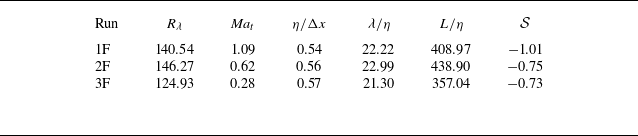
(Wang et al. Reference Wang, Wang, Xiao, Shi and Chen2010). We simulated a total of three flows with different steady-state turbulent Mach numbers:
 $\textit{Ma}_t = 1.08$
,
 $0.63$
and
 $0.28$
(referred to as 1F, 2F and 3F, respectively; where ‘F’ stands for forced). The steady Taylor-scale Reynolds number
 $R_\lambda$
is around
 $140$
for all runs. The key parameters characterizing the simulations are summarized in table 3. All average quantities in table 3 are computed by first taking the spatial average of the respective quantities at all
 $512^3$
grid points, followed by a temporal average during the steady-state phase. Time is normalized using the initial large-eddy turnover time,
 $\tau _0$
, in the following analysis.
Numerical setting and basic statistics of forced runs in the steady state.

Evolution of global statistics of forced runs. Red circle, blue square and magenta diamond lines refer to runs 1F, 2F and 3F, respectively. (a) The turbulent kinetic energy
 $\mathcal{K}$
normalized by its steady value
 $\mathcal{K}_s$
and the Kolmogorov scale
 $\eta$
divided by the grid length
 $\Delta x = 2\pi /512$
(shown in the inset). The horizontal dashed line in the figure marks the value of 1, and the horizontal dashed line in the inset marks the value of
 $0.5$
. (b) The Reynolds number on the Taylor microscale
 $R_\lambda$
. (c) The turbulent Mach number
 $\textit{Ma}_t$
. (d) The velocity gradient skewness
 $\mathcal{S}$
.

Figure 2 shows the evolution of global statistics for the forced runs. In all cases,
 $\eta / \Delta x$
remains above 0.5, and the integral scale
 $L$
stays around one-third of the computational domain size (not shown), indicating that the flow structures are satisfactorily resolved. The turbulent kinetic energy
 $\mathcal{K}$
, the Taylor-scale Reynolds number
 $R_\lambda$
, and the turbulent Mach number
 $\textit{Ma}_t$
all first grows from the initial flow, which has relatively small kinetic energy and dissipation. Then they experience a decline during
 $0.5 \leqslant t / \tau _0 \leqslant 1.5$
as viscous dissipation exceeds the power input from the external forcing. All flows reach a statistically steady state after approximately
 $14\tau _0$
. The velocity gradient skewness
 $\mathcal{S}$
in all forced runs is lower than the typical incompressible turbulence value of
 $\mathcal{S} \approx -0.5$
, which can be attributed to the strong compressibility effects, particularly the large negative velocity divergence near shocklets, as similarly observed by Wang et al. (Reference Wang, Wang, Xiao, Shi and Chen2010).
4. Numerical study of the energy flux
In this section, we begin by validating the SGS stress integral expression (2.9), and studying the total interscale energy transfers, see § 4.1. We then investigate the solenoidal, mixed and dilatational energy transfers, as well as the scaling of dilatational energy transfer as a function of the turbulent Mach number in § 4.2. Furthermore, in § 4.3, we conduct a systematic analysis of the contributions from local and non-local terms for each energy transfer mechanism, as defined in (2.11) and (2.13). Finally, we apply our results to the LES and discuss the tuning of its parameters in SGS viscosity model in § 4.4. The average interscale energy transfer terms,
 $\langle \varPi ^\ell _x \rangle$
(where
 $x$
can be
 $s1$
,
 $s2$
,
 $s3$
,
 $m1$
,
 $m2$
,
 $m3$
,
 $d$
and
 $l$
or
 $nl$
), are computed by taking the spatial average of the corresponding term
 $\varPi ^\ell _x$
at all
 $512^3$
points. For the freely decaying runs, this average is taken from a single snapshot, while for the forced runs, it is taken as the temporal average of three snapshots during the steady-state phase.
4.1. Validation of (2.9) and study of total interscale energy transfer
First, we validate the integral expression of SGS stress by calculating it using (2.1) and (2.9). The trapezoidal rule is employed for the numerical integration in (2.9), with sufficiently small steps to ensure convergence. The quantities obtained from the integral expressions differ from the definition (2.1), by the order of
 $1\,\%$
. Typical values of the norm of the differences are shown in table 4, at two values of
 $\ell$
. In addition, figure 3 shows the SGS stress
 $\tau _{11}^\ell$
in the plane
 $x=\pi$
for run 1D at
 $t/\tau _0 = 5.59$
, filtered at the scale
 $\ell = 15.50 \eta$
. In figure 3(a), we present the value of
 $\tau _{11}^\ell$
determined using the definition in (2.1), and in figure 3(b), the result obtained from the integral expression in (2.9). The comparison between the two panels shows that the integral expression (2.9), accurately captures the SGS stress as defined by (2.1), demonstrating the reliability of our numerical results.
Average relative errors (%) of the SGS stress calculated with the integral expression
 $\tau ^\ell _{\textit{ij},\textit{int}}$
with respect to the SGS stress calculated with the definition
 $\tau ^\ell _{\textit{ij},\textit{def}}$
, for the run 1D at
 $t/\tau _0 = 5.59$
.

A SGS stress
 $\tau _{11}^\ell$
of the section
 $x=\pi$
for the run 1D filtered at the scale
 $\ell = 15.50 \eta$
normalized by the kinetic energy
 $\mathcal{K} = \langle \rho u_i u_i \rangle /2$
. Both panels use the same colour map. (a) With the definition
 $\tau ^\ell _{11,\textit{def}}$
. (b) With the integral expression
 $\tau ^\ell _{11,\textit{int}}$
.

Total interscale energy transfer
 $\langle \varPi ^\ell \rangle$
as a function of filtering scale
 $\ell$
. All quantities are normalized by the average energy dissipation rate
 $\varepsilon$
. (a) At
 $t/\tau _0 = 5.59$
for run 1D (red), and in the steady state for run 1F (blue). Solid lines represent the energy transfer calculated from the definition
 $\varPi ^\ell _{\textit{def}} \equiv \tau _{\textit{ij}}^\ell ({\partial \widetilde {u_i}^{\ell }}/{\partial x_j})$
. Circle and square symbols represent the energy transfer calculated from the integral expression
 $\varPi ^\ell _{{int}}$
in (2.10). The difference between the two expressions does not exceed
 ${\sim}2 \,\%$
. (b) The energy transfer terms at different times for run 1D.

Figure 4(a) illustrates the dependence of the total interscale energy transfer,
 $\langle \varPi ^\ell \rangle$
, on the filtering scale
 $\ell$
for run 1D at
 $t/\tau _0 = 5.59$
and for run 1F in the steady state. The solid lines represent calculations based on the definition
 $\varPi ^\ell _{\textit{def}} \equiv \tau _{\textit{ij}}^\ell ({\partial \widetilde {u_i}^{\ell }}/{\partial x_j})$
, while the symbols correspond to the results obtained from the integral expression in (2.10). Across all runs and filtering scales, the solid lines and symbols agree within
 $2\,\%$
, further validating the accuracy of the numerical integration of the SGS stress. A similar agreement was observed for all other runs (not shown).
Additionally, we observe that in the forced steady-state turbulence, the maximum of
 $|\langle \varPi ^\ell \rangle /\varepsilon |$
approaches
 $1$
, consistent with the results from turbulence simulations by Johnson (Reference Johnson2020) (see figure 2 in that article). In contrast, for freely decaying runs, this ratio is significantly smaller than
 $1$
. This difference can be attributed to the distinct set-ups of two types of turbulence. In forced steady-state turbulence, energy is continuously injected at large scales, maintaining a balance between energy transfer,
 $\langle \varPi ^\ell \rangle$
, and dissipation,
 $\varepsilon$
. Conversely, in freely decaying turbulence, energy transferred through a given scale in the inertial range is dissipated at smaller scales later. As a result, the energy transfer rate at any scale is always lower than the dissipation rate at any given time, due to the overall energy decline. Moreover, as the Taylor scale Reynolds number,
 $R_\lambda$
, decreases, viscosity effects become more pronounced, further reducing the peak values of
 $| \langle \varPi ^\ell \rangle /\varepsilon |$
. This trend is evident in figure 4(b), which depicts energy transfer at four different time instances for run 1D. As time progresses and
 $R_\lambda$
decreases, the peak value of value of
 $| \langle \varPi ^\ell \rangle /\varepsilon |$
as a function of
 $\ell$
also diminishes. Notably, the values of
 $R_\lambda \approx 400$
studied by Johnson (Reference Johnson2020) are higher than those in our simulations.
4.2. Solenoidal, mixed and dilatational contribution to interscale energy flux
In this subsection, we analyse the solenoidal, mixed and dilatational energy flux and study the relationship between mixed and dilatational energy transfer and the turbulent Mach number.
Terms of interscale energy transfer as a function of filtering scale
 $\ell$
. The solid lines indicate forced runs in the steady state, with red, blue and magenta representing, respectively, runs 1F (
 $\textit{Ma}_t = 1.09$
), 2F (
 $\textit{Ma}_t = 0.63$
) and 3F (
 $\textit{Ma}_t = 0.28$
). The dashed lines indicate freely decaying runs at
 $t/\tau _0 = 5.59$
, with red, blue, magenta and orange representing, respectively, runs 1D (
 $\textit{Ma}_t = 0.33$
), 2D (
 $\textit{Ma}_t = 0.22$
), 3D (
 $\textit{Ma}_t = 0.11$
), 4D (
 $\textit{Ma}_t = 0.03$
). All curves are normalized by the average energy dissipation rate
 $\epsilon$
. (a) Solenoidal energy transfer
 $\langle \varPi ^\ell _{s} \rangle$
. (b) Mixed energy transfer
 $\langle \varPi ^\ell _m \rangle$
. (c) Dilatational energy transfer
 $\langle \varPi ^\ell _{d} \rangle$
.

Figure 5 shows the dependence on filtering scale,
 $\ell$
, of the various contributions to interscale energy transfer. Specifically, figure 5(a) shows the contribution due to the solenoidal motion,
 $\varPi ^\ell _{s}$
, figure 5(b) shows the contribution due to the mixed interaction,
 $\varPi ^\ell _m$
, and figure 5(c) shows the contribution induced by purely dilatational motion,
 $\varPi ^\ell _{d}$
. The terms
 $ \langle \varPi ^\ell _m \rangle$
and
 $ \langle \varPi ^\ell _{d} \rangle$
are very close to zero for run 4D (
 $\textit{Ma}_t = 0.03$
), which can be considered as nearly incompressible, and increase with the turbulent Mach number. Across all runs,
 $ \langle \varPi ^\ell _{s} \rangle$
is significantly larger than both
 $ \langle \varPi ^\ell _m \rangle$
and
 $ \langle \varPi ^\ell _{d} \rangle$
, indicating that the energy transfer is mostly due to the solenoidal motion. Furthermore, all terms are negative at small scales (
 $\ell \ll L$
), demonstrating that in the three-dimensional compressible turbulences simulated here, all terms contribute to an energy cascade from large to small scales.
The maximum interscale energy transfer
 $\max _\ell |\langle \varPi ^{\ell }_x \rangle /\varepsilon |$
as a function of turbulent Mach number
 $\textit{Ma}_t$
. Both axes are in a logarithmic scale at
 $t/\tau =5.59$
. The square symbol indicates forced runs in the steady state, with red, blue and magenta representing, respectively, runs 1F, 2F and 3F. The circle symbol indicates freely decaying runs at
 $t/\tau _0 = 5.59$
, with red, blue, magenta and orange representing, respectively, runs 1D, 2D, 3D and 4D. (a) Mixed energy transfer
 $\max _\ell |\langle \varPi ^{\ell }_m \rangle /\varepsilon |$
. The black dashed line is
 $0.44 \textit{Ma}_t^2$
. (b) Dilatational energy transfer
 $\max _\ell |\langle \varPi ^{\ell }_d \rangle /\varepsilon |$
. The black dashed line is
 $1.46 \textit{Ma}_t^4$
.

For each run at each snapshot, we compute the maximum interscale energy transfer
 $| \langle \varPi ^{\ell }_x \rangle /\varepsilon |$
over
 $\ell$
, i.e.
 $\max _\ell | \langle \varPi ^{\ell }_x \rangle /\varepsilon |$
, with
 $x=m$
and
 $d$
. Figures 6(a) and 6(b) show this maximum value as a function of the turbulent Mach number. Both
 $\max _\ell | \langle \varPi ^{\ell }_m \rangle /\varepsilon |$
and
 $\max _\ell | \langle \varPi ^{\ell }_d \rangle /\varepsilon |$
are increasing functions of the turbulent Mach number. For freely decaying runs with small Mach numbers (
 $\textit{Ma}_t \lesssim 0.3$
), the data in figure 6(a) can be fitted as
 $\max _\ell | \langle \varPi ^{\ell }_m \rangle /\varepsilon | \approx 0.44 \textit{Ma}_t^2$
, and the data in figure 6(b) as
 $| \langle \varPi ^{\ell }_d \rangle /\varepsilon | \approx 1.46 \textit{Ma}_t^4$
. The prefactors in these scaling laws may be related with the flow field configuration and the Reynolds number. Notably, the
 $\textit{Ma}_t^4$
scaling of the dilatational energy transfer aligns with the scaling law of
 $\varepsilon _d /\varepsilon _s \sim \textit{Ma}_t^4$
, where
 $\varepsilon _d$
and
 $\varepsilon _s$
are, respectively, the dilatational and solenoidal dissipation, obtained from the pseudosound relationship by Ristorcelli (Reference Ristorcelli1997). This suggests that for our low-Mach-number runs, turbulence behaviour could be described by the pseudosound theory. However, for the forced runs and run 1D, the increase in mixed and dilatational interscale energy transfer with turbulent Mach number deviates from the scaling law and indicates a slower growth rate, suggesting that the observed scaling relations apply primarily in the low-
 $\textit{Ma}_t$
regime of compressible turbulence, with a turbulent Mach number
 $\textit{Ma}_t \lesssim 0.3$
.
4.3. Local and non-local contribution of each action to the energy transfer
In this subsection, we study separately the contribution of local and non-local term of each action, as defined in (2.11) and (2.13), to the solenoidal, mixed and dilatational interscale energy transfer.
Terms of the solenoidal energy transfer as a function of filtering scale
 $\ell$
for the runs, normalized by the sum of these terms
 $\langle \varPi ^\ell _s \rangle$
. The grey dashed line indicates the Taylor scale
 $\ell = \lambda$
. (a) Run 1D (
 $\textit{Ma}_t = 0.33$
) at
 $t/\tau _0 = 5.59$
. (b) Run 1F (
 $\textit{Ma}_t = 1.09$
) in the steady state.

The ratio of terms for
 $\varPi ^{\ell }_{s}$
as a function of filtering scale
 $\ell$
. The solid line indicates forced runs, with red, blue,and magenta representing, respectively, runs 1F (
 $\textit{Ma}_t = 1.09$
), 2F (
 $\textit{Ma}_t = 0.63$
) and 3F (
 $\textit{Ma}_t = 0.28$
). The dash–dotted line indicates freely decaying runs, with red, blue, magenta and orange representing, respectively, runs 1D (
 $\textit{Ma}_t = 0.33$
), 2D (
 $\textit{Ma}_t = 0.22$
), 3D (
 $\textit{Ma}_t = 0.11$
), 4D (
 $\textit{Ma}_t = 0.03$
). The circle and square symbols represent the value at the Taylor scale for forced runs and freely decaying runs, respectively. (a) The ratio of
 $\langle \varPi ^\ell _{s1,l} \rangle / \langle \varPi ^\ell _{s2,l} \rangle$
. (b) The ratio of
 $\langle \varPi ^\ell _{s1,nl} \rangle / \langle \varPi ^\ell _{s2,nl} \rangle$
.

Figure 7 shows the contribution of each term to the solenoidal interscale energy transfer, as studied in the incompressible case (Johnson Reference Johnson2020; Yang et al. Reference Yang, Zhou, Xu and He2023). Figure 7(a) shows the results for run 1F in the steady state, and figure 7(b) for run 1D at
 $t/\tau =5.59$
. Similar trends are observed for all other runs. The overall behaviour in figure 7 aligns with figure 3 of Johnson (Reference Johnson2020). At small scales (
 $\ell \approx \eta$
), the energy transfer is dominated by local terms, the non-local terms being comparatively small. However, at larger scales (
 $\ell \gg \eta$
), non-local contributions become more significant. Specifically, for all freely decaying runs, as shown in figure 7(a) as an example, non-local contributions
 $ \langle \varPi ^\ell _{s,nl} \rangle$
accounting for more in the solenoidal interscale energy transfer, with
 $ \langle \varPi ^\ell _{s,l} \rangle : \langle \varPi ^\ell _{s,nl} \rangle \approx 2 : 5$
at the Taylor scale. For all forced runs, as shown in figure 7(b) as an example, non-local terms remain slightly dominant, with a ratio
 $ \langle \varPi ^\ell _{s,l} \rangle : \langle \varPi ^\ell _{s,nl} \rangle \approx 2 : 3$
at the Taylor scale. These results differ from those of Johnson (Reference Johnson2020), who found that
 $ \langle \varPi ^\ell _{s,l} \rangle \approx \langle \varPi ^\ell _{s,nl} \rangle$
in the inertial range. The discrepancy may be attributed to the different Reynolds numbers (with
 $R_\lambda \approx 140$
for forced runs and
 $R_\lambda \lt 100$
for freely decaying runs in our work, versus
 $R_\lambda \approx 400$
in Johnson Reference Johnson2020) and the different flow types (compressible turbulence here versus incompressible turbulence in Johnson Reference Johnson2020), which may influence the structure of the large-scale flow (Yang, Pumir & Xu Reference Yang, Pumir and Xu2018).
We then study the contribution of each interaction, i.e. strain amplification(
 $s1$
), vorticity amplification(
 $s2$
) and strain–vorticity correlation (
 $s3$
), to solenoidal energy transfer. For scale-local interactions, figure 8(a) shows that the ratio of
 $ \langle \varPi ^\ell _{s1,l} \rangle / \langle \varPi ^\ell _{s2,l} \rangle$
increases with Mach number. At low Mach numbers, this ratio is close to the incompressible limit of
 $3$
, predicted by the Betchov identities (Betchov Reference Betchov1956) of incompressible turbulence. For scale non-local interactions, figure 8(b) shows that the ratio of
 $ \langle \varPi ^\ell _{s1,nl} \rangle / \langle \varPi ^\ell _{s2,nl} \rangle$
also increases with Mach number. For low-Mach number-runs (run 3D with
 $\textit{Ma}_t=0.11$
and run 4D with
 $\textit{Ma}_t=0.03$
), this ratio approaches
 $1$
, consistent with the numerical observations of Johnson (Reference Johnson2020) and the theoretical discussion of Yang et al. (Reference Yang, Zhou, Xu and He2023), who both found
 $ \langle \varPi ^\ell _{s1,nl} \rangle / \langle \varPi ^\ell _{s2,nl} \rangle \approx 1$
for incompressible turbulence. In all cases, we find that for both scale-local and scale non-local actions, compressibility enhances strain self-amplification, increasing the contribution of
 $ \langle \varPi ^\ell _{s1} \rangle$
to solenoidal energy transfer.
Terms of the interscale energy transfer between the solenoidal part and the dilatational part as a function of filtering scale
 $\ell$
, normalized by the sum of these terms
 $\langle \varPi ^\ell _m \rangle$
. The grey dashed line indicates the Taylor scale
 $\ell = \lambda$
. (a) Run 1D (
 $\textit{Ma}_t = 0.33$
) at
 $t/\tau _0 = 5.59$
. (b) Run 1F (
 $\textit{Ma}_t = 1.09$
) in the steady state.

The ratio of
 $\langle \varPi ^\ell _{m1,nl} \rangle / \langle \varPi ^\ell _{m2,nl} \rangle$
as a function of filtering scale solid line indicates forced runs, with red, blue and magenta representing, respectively, runs 1F (
 $\textit{Ma}_t = 1.09$
), 2F (
 $\textit{Ma}_t = 0.63$
) and 3F (
 $\textit{Ma}_t = 0.28$
), and the dash–dotted line indicates freely decaying runs, with red and blue representing, respectively, runs 1D (
 $\textit{Ma}_t = 0.33$
) and 2D (
 $\textit{Ma}_t = 0.22$
). The circle and square symbols represent the value at the Taylor scale for forced runs and freely decaying runs, respectively.

Figure 9 shows the relative contributions of each term to mixed interscale energy transfer. Figure 9(a) represents run 1D at
 $t / \tau_0 = 5.59$
, and figure 9(b) represents run 1F in the steady state. Similar figures are found for all the other runs. At small scales (
 $\ell \approx \eta$
), the local terms
 $ \langle \varPi ^\ell _{m1,l} \rangle$
and
 $ \langle \varPi ^\ell _{m2,l} \rangle$
dominate the mixed energy transfer, with a fix ratio
 $ \langle \varPi ^\ell _{m1,l} \rangle : \langle \varPi ^\ell _{m2,l} \rangle = 2:1$
defined by (2.14c
). At large scales (
 $\ell \gg \eta$
), non-local contributions
 $ \langle \varPi ^\ell _{m,nl} \rangle$
become dominant, with a ratio
 $ \langle \varPi ^\ell _{m,l} \rangle : \langle \varPi ^\ell _{m,nl} \rangle \approx 2:3$
at the Taylor scale for all runs. Figure 10 shows the ratio of
 $ \langle \varPi ^\ell _{m1,nl} \rangle / \langle \varPi ^\ell _{m2,nl} \rangle$
as a function of
 $\ell$
, which is always above 1, signifying that
 $ \langle \varPi ^\ell _{m1,nl} \rangle$
contributes always more than
 $ \langle \varPi ^\ell _{m2,nl} \rangle$
. The ratio
 $ \langle \varPi ^\ell _{m1,nl} \rangle / \langle \varPi ^\ell _{m2,nl} \rangle$
tends to increase with the Mach number. For low-Mach-number flows (run
 $2D$
with
 $\textit{Ma}_t=0.22$
), this ratio is close to the limit of
 $1$
at the Taylor scale. Furthermore, the interaction between dilatation and vorticity, described by the term
 $ \langle \varPi ^{\ell }_{m3,l} \rangle$
and
 $ \langle \varPi ^{\ell }_{m3,nl} \rangle$
, contribute both very little to the energy transfer. This is consistent with previous observations that vorticity and dilatation are uncorrelated in compressible homogeneous turbulence and have small contribution to energy transfer (Erlebacher & Sarkar Reference Erlebacher and Sarkar1993; Wang et al. Reference Wang, Shi, Wang, Xiao, He and Chen2012a
; Yang et al. Reference Yang, Fang, Fang, Pumir and Xu2022).
The ratio of
 $\langle \varPi ^\ell _{d,nl} \rangle / \langle \varPi ^\ell _{d} \rangle$
as a function of filtering scale
 $\ell$
. The solid line indicates forced runs, with red, blue and magenta representing, respectively, runs 1F (
 $\textit{Ma}_t = 1.09$
), 2F (
 $\textit{Ma}_t = 0.63$
) and 3F (
 $\textit{Ma}_t = 0.28$
), and the dash–dotted line indicates freely decaying runs, with red and blue representing, respectively, runs 1D (
 $\textit{Ma}_t = 0.33$
) and 2D (
 $\textit{Ma}_t = 0.22$
). The circle and square symbols represent the value at the Taylor scale for forced runs and freely decaying runs, respectively. The black dashed line indicates the value of
 $0.5$
.

Figure 11 shows the relative contributions of the non-local term to the dilatational interscale energy transfer, i.e. the ratio
 $\langle \varPi _{d,nl}^{\ell } \rangle / \langle \varPi _{d}^{\ell } \rangle$
. The corresponding local contribution is given by
 ${\langle \varPi _{d,l}^{\ell } \rangle }/{ \langle \varPi _{d}^{\ell } \rangle }= 1- {\langle \varPi _{d,nl}^{\ell } \rangle }/{\langle \varPi _{d}^{\ell } \rangle }$
. Similar to
 $\langle \varPi ^\ell _s \rangle$
and
 $\langle \varPi ^\ell _m \rangle$
, the local contribution dominates at small scales (
 $\ell \approx \eta$
), and decreases with increasing
 $\ell$
, while the non-local contribution is close to
 $0$
at small scales and increases with
 $\ell$
. Additionally, the ratio of local and non-local contribution is
 $ \langle \varPi ^\ell _{d,l} \rangle : \langle \varPi ^\ell _{d,nl} \rangle \approx 1:1$
at the Taylor scale.
4.4. Application to LES modelling
In this subsection, we apply our study of interscale energy flux to the functional SGS model in the LES of compressible flows and analyse the limitations of commonly applied models.
Under the Boussinesq eddy-viscosity assumption (Boussinesq Reference Boussinesq1877), and by using the widely adopted Smagorinsky model (Smagorinsky Reference Smagorinsky1963) for the eddy-viscosity of the deviatoric SGS tensor, as well as the Yoshizawa model (Yoshizawa Reference Yoshizawa1986) for the isotropic part of the SGS tensor, we could obtain
 \begin{equation} \tau ^\ell _{\textit{ij}} = -2 \overline {\rho }^\ell C_S^2 \Delta ^2 |\widetilde {S}^\ell | \widetilde {S}_{\textit{ij}}^\ell + \frac {2}{3} \overline {\rho }^\ell C_I \Delta ^2 |\widetilde {S}^\ell |^2 \delta _{\textit{ij}}, \end{equation}
where
 $C_S$
and
 $C_I$
are constants,
 $\Delta$
is the filter cutoff length and
 \begin{equation} |\widetilde {S}^\ell | = \sqrt {2 \left (\widetilde {S}_{\textit{ij}}^\ell \widetilde {S}_{\textit{ij}}^\ell + \frac {1}{3}\widetilde {A}_{\textit{ll}}^\ell \widetilde {A}_{\textit{ll}}^\ell \right )}. \end{equation}
Substituting this model into the definition of interscale energy transfer yields the modelled interscale energy transfer,
 \begin{equation} \varPi ^\ell _{\textrm {LES}} = -2 \overline {\rho }^\ell C_S^2 \Delta ^2 |\widetilde {S}^\ell | \widetilde {S}_{\textit{ij}}^\ell \widetilde {S}_{\textit{ij}}^\ell + \frac {2}{3} \overline {\rho }^\ell C_I \Delta ^2 |\widetilde {S}^\ell |^2 \widetilde {A}^\ell _{\textit{ll}}. \end{equation}
The first term represents energy transfer arising from the interaction between the deviatoric component of the filtered velocity gradient tensor (
 $\widetilde {S}_{\textit{ij}}^\ell$
) and the deviatoric part of the SGS stress. This corresponds to the terms
 $\varPi _{s1}^\ell + \varPi _{s2}^\ell + \varPi _{s3}^\ell + \varPi _{m1}^\ell$
in (2.10). The second term originates from the interaction between the isotropic component of the filtered velocity gradient (
 $\widetilde {A}_{\textit{kk}}^\ell \delta _{\textit{ij}}$
) and the isotropic part of the SGS stress, corresponding to
 $\varPi _{m2}^\ell + \varPi _{m3}^\ell + \varPi _{d}^\ell$
in (2.10).
This LES model is theoretically valid only if the actual interscale energy transfer and the modelled interscale energy transfer are equivalent. For the chosen filtering scale
 $\ell$
, we conclude that
 \begin{equation} \frac {\left \langle -2 \overline {\rho }^\ell C_S^2 \Delta ^2 |\widetilde {S}^\ell | \widetilde {S}_{\textit{ij}}^\ell \widetilde {S}_{\textit{ij}}^\ell \right \rangle }{\left \langle \frac {2}{3} \overline {\rho }^\ell C_I \Delta ^2 |\widetilde {S}^\ell |^2 \widetilde {A}^\ell _{\textit{ll}} \right \rangle } = \frac {\left \langle \varPi _{s1}^\ell +\varPi _{s2}^\ell +\varPi _{s3}^\ell +\varPi _{m1}^\ell \right \rangle }{\left \langle \varPi _{m2}^\ell +\varPi _{m3}^\ell +\varPi _{d}^\ell \right \rangle }, \end{equation}
from which, a relation between the constants
 $C_I$
and
 $C_S$
can be deduced,
 \begin{equation} \frac {C_I}{C_S^2} = - \frac {3\big\langle \overline {\rho }^\ell \widetilde {S}_{\textit{ij}}^\ell \widetilde {S}_{\textit{ij}}^\ell \big \rangle \left \langle \varPi _{m2}^\ell +\varPi _{m3}^\ell +\varPi _{d}^\ell \right \rangle }{ \left \langle \overline {\rho }^\ell |\widetilde {S}^\ell | \widetilde {A}^\ell _{\textit{ll}} \right \rangle \left \langle \varPi _{s1}^\ell +\varPi _{s2}^\ell +\varPi _{s3}^\ell +\varPi _{m1}^\ell \right \rangle }. \end{equation}
The ratio
 $C_I/C_S^2$
calculated according to (4.5) as a function of filtering scale
 $\ell$
. The solid line indicates forced runs, with red, blue and magenta representing, respectively, runs 1F (
 $\textit{Ma}_t = 1.09$
), 2F (
 $\textit{Ma}_t = 0.63$
) and 3F (
 $\textit{Ma}_t = 0.28$
). The dash–dotted line indicates freely decaying runs, with red and blue representing respectively runs 1D (
 $\textit{Ma}_t = 0.33$
) and 2D (
 $\textit{Ma}_t = 0.22$
). The circle and square symbols represent the value at the Taylor scale for forced runs and freely decaying runs, respectively. The black dashed line indicates the value of
 $5$
.

For our numerical cases, figure 12 shows the evolution of the ratio
 $C_I/C_S^2$
calculated by (4.5) as a function of the filtering scale
 $\ell$
for both forced and freely decaying runs. Despite the differences in flow types (freely decaying versus forced) and turbulent Mach numbers, the ratio
 $C_I/C_S^2$
remains consistently around
 $5$
for all runs at scales below the Taylor microscale. Zang, Dahlburg & Dahlburg (Reference Zang, Dahlburg and Dahlburg1992) investigated the influence of the model constants
 $C_I$
and
 $C_S$
, testing
 $C_I/C_S^2$
over a range of 0–30, and concluded that it is challenging to identify universal values for the modelling constants
 $C_I$
and
 $C_S$
across different types of turbulence regimes and Mach number ranges. Our observed ratio of
 $C_I/C_S^2 \approx 5$
falls within this range, and provides a practical criterion for tuning the model parameters.
5. Concluding remarks
In summary, we derived an integral expression for SGS stress in compressible turbulence and introduced a methodology to analyse interscale energy transfer. This framework allows us to formally decompose the kinetic energy transfer into components associated with solenoidal motion, solenoidal–dilatational interaction and dilatational motion, which are further categorized into scale-local and non-local contributions.
Our theoretical decomposition has been validated through DNS of freely decaying and forced compressible turbulence. The results reveal that the proportion of mixed and dilatational energy transfer increases with turbulent Mach number. Additionally, for weakly compressible turbulence, we observed that
 $\max _\ell |\langle \varPi ^{\ell }_m \rangle /\varepsilon |$
and
 $\max _\ell |\langle \varPi ^{\ell }_d \rangle /\varepsilon |$
scale with the turbulent Mach number as
 $\textit{Ma}_t^2$
and
 $ \textit{Ma}_t^4$
, respectively, influence of compressibility on energy transfer dynamics. Furthermore, we examined the contribution of local and non-local terms for each action in the energy transfer and analysed their variation with the turbulent Mach number. Our study also extends to the commonly used Smagorinsky and Yoshizawa models for the compressible LES, providing criteria for parameter tuning in these models.
Funding
P.-F.Y., H.X., L.F. and J.F. acknowledge support from the National Natural Science Foundation of China (NSFC) under grants 12202452, 11672157, 91852104, 12372214 and 23FAA01491. P.-F.Y. also acknowledges support from the Fundamental Research Funds for Central University (D5000240110). A.P. was supported by the French Agence Nationale de la Recherche under contract no. ANR-20-CE30-0035 (project TILT), and is thankful to the Max Planck Institute for Dynamics and Self-organisation (Göttingen, Germany) for its continuous support.
Declaration of interest
The authors report no conflict of interest.