1. Introduction
Since the pioneering work of Kolmogorov (Reference Kolmogorov1941) (hereafter denoted K41), the turbulent energy dissipation rate
 $\overline{{\it\epsilon}}$
has been considered to be a cornerstone quantity in the study of turbulence, especially in the context of the small-scale motion(or SSM). Batchelor & Townsend (Reference Batchelor and Townsend1947) and Townsend (Reference Townsend1951) measured moments of first- and higher-order spatial derivatives of the longitudinal velocity fluctuation
 $u$
to characterize the behaviour of the SSM in decaying turbulence downstream of a grid. The transport equation for
 $\overline{{\it\epsilon}}$
, first written by von Kármán (Reference von Kármán1937), see also von Kármán & Howarth (Reference von Kármán and Howarth1938), for decaying homogeneous and isotropic turbulence (HIT) is given by
 $$\begin{eqnarray}-U\frac{\text{d}\overline{{\it\epsilon}}}{\text{d}x}=2{\it\nu}\overline{\left({\it\omega}_{i}{\it\omega}_{j}\frac{\partial u_{i}}{\partial x_{j}}\right)}-2{\it\nu}^{2}\overline{\left(\frac{\partial {\it\omega}_{i}}{\partial x_{j}}\right)\left(\frac{\partial {\it\omega}_{i}}{\partial x_{j}}\right)},\end{eqnarray}$$
where
 $U$
is the (constant) mean velocity in the
 $x_{1}$
direction,
 ${\it\omega}_{i}$
the fluctuating vorticity component along the
 $x_{i}$
direction, and
 ${\it\nu}$
is the fluid kinematic viscosity (the overbar denotes time averaging). In this paper,
 $u_{1}$
,
 $u_{2}$
, and
 $u_{3}$
will be used interchangeably with
 $u$
,
 $v$
,
 $w$
; similarly for
 $x_{1}$
,
 $x_{2}$
,
 $x_{3}$
and
 $x$
,
 $y$
,
 $z$
. Equation (1.1) states that the difference between the production of
 $\overline{{\it\epsilon}}$
(first term on the right of (1.1)), or creation of
 $\overline{{\it\epsilon}}$
through the stretching of vorticity by the turbulent strain field, and dissipation or destruction of
 $\overline{{\it\epsilon}}$
(second term on the right of (1.1)) through the action of viscosity, is balanced by the streamwise rate of decay of
 $\overline{{\it\epsilon}}$
(first term on the left of (1.1)).
Batchelor & Townsend (Reference Batchelor and Townsend1947) were first to test the isotropic form of (1.1), viz.
 $$\begin{eqnarray}-U\frac{\text{d}\overline{{\it\epsilon}}_{iso}}{\text{d}x}=\frac{7}{3\sqrt{15}}\frac{{\overline{{\it\epsilon}}_{iso}}^{3/2}}{{\it\nu}^{1/2}}\left[S_{1,1}+2\frac{G}{R_{{\it\lambda}}}\right]\end{eqnarray}$$
in decaying grid turbulence. In (1.2),
 $S_{1,1}$
(
 ${<}0$
) is the skewness of
 $\partial u_{1}/\partial x_{1}$
 $$\begin{eqnarray}S_{1,1}=\frac{\overline{(\partial u_{1}/\partial x_{1})^{3}}}{\overline{(\partial u_{1}/\partial x_{1})^{2}}^{3/2}},\end{eqnarray}$$
 $G$
is the non-dimensional enstrophy destruction coefficient of
 $\overline{{\it\epsilon}}_{iso}$
 $$\begin{eqnarray}G=\overline{u_{1}^{2}}\frac{\overline{(\partial ^{2}u_{1}/\partial x_{1}^{2})^{2}}}{\overline{(\partial u_{1}/\partial x_{1})^{2}}^{2}},\end{eqnarray}$$
and
 $R_{{\it\lambda}}$
is the Taylor microscale Reynolds number
 $$\begin{eqnarray}R_{{\it\lambda}}=\frac{\overline{u^{2}}^{1/2}{\it\lambda}}{{\it\nu}}\end{eqnarray}$$
with the Taylor microscale
 ${\it\lambda}$
defined as the ratio
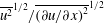 $\overline{u^{2}}^{1/2}/\overline{(\partial u/\partial x)^{2}}^{1/2}$
. If a power-law decay rate for the longitudinal velocity variance is assumed, viz.
 $\overline{u^{2}}\sim x^{-n}$
, then (1.2) can be rewritten as (e.g. Antonia et al.
Reference Antonia, Zhou, Danaila and Anselmet2000b
)
 $$\begin{eqnarray}\frac{90}{7(1+2R)}\left(\frac{n+1}{n}\right)\frac{1}{R_{{\it\lambda}}}=S_{1,1}+2\frac{G}{R_{{\it\lambda}}},\end{eqnarray}$$
where
 $R=\overline{v^{2}}/\overline{u^{2}}$
. This equation represents, in essence, a constraint on how
 $S_{1,1}$
varies with
 $R_{{\it\lambda}}$
. It was first derived by Batchelor & Townsend (Reference Batchelor and Townsend1947) from (1.1) with
 $R=1$
and
 $n=1$
. Since the ratio
 $G/R_{{\it\lambda}}$
approaches a constant relatively rapidly with increasing
 $R_{{\it\lambda}}$
(evidence for this was collected by Lee et al.
Reference Lee, Djenidi, Antonia and Danaila2013) and the term on the left-hand side of (1.6) must eventually vanish, (1.6) implies that the magnitude of
 $S_{1,1}$
should become constant at sufficiently large
 $R_{{\it\lambda}}$
. This is consistent with K41 and also the prediction of Qian (Reference Qian1994), but in contradiction with the modified similarity hypothesis of Kolmogorov (Reference Kolmogorov1962) or K62. This latter hypothesis has spawned tremendous interest in how normalized high-order moments of
 $\partial u_{1}/\partial x_{1}$
vary with
 $R_{{\it\lambda}}$
(e.g. Van Atta & Antonia Reference Van Atta and Antonia1980; Sreenivasan & Antonia Reference Sreenivasan and Antonia1997; Ishihara et al.
Reference Ishihara, Kaneda, Yokokawa, Itakura and Uno2007).
In a recent paper, Thiesset, Antonia & Djenidi (Reference Thiesset, Antonia and Djenidi2014) showed that along the axis in the self-preserving far field of a round jet, the transport equation for
 $\overline{{\it\epsilon}}_{iso}$
can be cast in the same form as (1.6), i.e. the term on the left-hand side can be written as
 $C/R_{{\it\lambda}}$
, where
 $C$
is a constant, which may depend on the initial and boundary conditions (IBC) of the flow. They also pointed out that this constant will differ in different flows so that
 $S_{1,1}+2G/R_{{\it\lambda}}$
will approach its stationary state (
 $S_{1,1}+2G/R_{{\it\lambda}}=0$
) along different paths in each flow.
The present paper aims to provide some insight into the transport equation for
 $\overline{{\it\epsilon}}_{iso}$
along the centreline of a fully developed turbulent channel flow. This flow has received a significant amount of attention both experimentally (Laufer Reference Laufer1954; Comte-Bellot Reference Comte-Bellot1963) and via direct numerical simulations (DNS) (Kim, Moin & Moser Reference Kim, Moin and Moser1987; Kim Reference Kim1989). Various aspects of the SSM have been examined in some detail (Antonia, Kim & Browne Reference Antonia, Kim and Browne1991; Kim & Antonia Reference Kim and Antonia1993; Antonia, Abe & Kawamura Reference Antonia, Abe and Kawamura2009; Vreman & Kuerten Reference Vreman and Kuerten2014b
) at different locations in this flow. The SSM has been found to approach local isotropy when the effect of the mean strain rate
 $\partial U/\partial y$
becomes small. On the centreline, the ratio
 $\overline{{\it\epsilon}}_{iso}/\overline{{\it\epsilon}}$
is sufficiently close to 1 (Antonia et al.
Reference Antonia, Kim and Browne1991, Reference Antonia, Abe and Kawamura2009) to allow us to consider the isotropic form of the transport equation of
 $\overline{{\it\epsilon}}$
. This flow is homogeneous in the
 $x_{1}$
direction so that there is no advection of
 $\overline{{\it\epsilon}}$
along
 $x_{1}$
. It is hence different from decaying-type flows such as grid turbulence, jets and wakes. The one-point energy budget at the centreline indicates that
 $\overline{{\it\epsilon}}$
is balanced by the turbulent transport of
 $\overline{q^{2}}$
(
 $\equiv \overline{u_{i}u_{i}}$
) by
 $u_{2}$
(Danaila et al.
Reference Danaila, Anselmet, Zhou and Antonia2001). One then expects the large-scale inhomogeneous term in the two-point energy budget equation for
 $\overline{({\rm\Delta}q)^{2}}$
(
 $=\overline{({\rm\Delta}u)^{2}}+\overline{({\rm\Delta}v)^{2}}+\overline{({\rm\Delta}w)^{2}}$
) to reflect the physics associated with this turbulent transport. By considering the limit at small separations of the two-point energy budget equation, a transport equation for
 $\overline{{\it\epsilon}}_{iso}$
can be obtained. The dependence of
 $S_{1,1}$
on
 $R_{{\it\lambda}}$
which ensues from this equation can then be compared with both measured and DNS values of
 $S_{1,1}$
.
This paper is structured as follows. In § 2, we derive the transport equation for
 $\overline{{\it\epsilon}}_{iso}$
. Details associated with the measurements are described in § 3, whilst the accuracy of quantities associated with the SSM is discussed in § 4. Section 4 also contains an assessment of local isotropy, in the specific context of the transport equation for
 $\overline{{\it\epsilon}}$
. An appropriate scaling for the transport equation for
 $\overline{{\it\epsilon}}_{iso}$
, which is discussed in § 5, yields an exact relation between
 $S_{1,1}$
,
 $G$
and
 $R_{{\it\lambda}}$
. This relation is compared to that of decaying HIT, ‘stationary’ forced periodic box turbulence (SFPBT), and along the axis in the far field of a round jet. A concluding discussion is given in § 6.
2. Transport equation for
 $\overline{{\it\epsilon}}_{iso}$

Danaila et al. (Reference Danaila, Anselmet, Zhou and Antonia2001) showed that, on the centreline of a fully developed channel flow, the isotropic form of the scale-by-scale energy budget equation is given by
 $$\begin{eqnarray}-\frac{6}{r^{4}}\int _{0}^{r}s^{4}\left[\frac{\partial \overline{u_{2}({\rm\Delta}u_{1})^{2}}}{\partial x_{2}}\right]\,\text{d}s-\overline{({\rm\Delta}u_{1})^{3}}+6{\it\nu}\frac{\partial }{\partial r}\overline{({\rm\Delta}u_{1})^{2}}=\frac{4}{5}\overline{{\it\epsilon}}r,\end{eqnarray}$$
where
 $s$
is a dummy variable. Note that
 $\overline{{\it\epsilon}}$
is identified here with
 $\overline{{\it\epsilon}}_{iso}=15{\it\nu}\overline{(\partial u_{1}/\partial x_{1})^{2}}$
;
 ${\rm\Delta}u_{1}=u_{1}(x_{1}+r)-u_{1}(x_{1})$
is the increment between longitudinal velocity fluctuations at two points separated by a distance
 $r$
. Equation (2.1) can be thought of as the generalized form of Kolmogorov’s equation (Kolmogorov Reference Kolmogorov1941). It contains a large-scale forcing term (first term on the left-hand side) which arises from the turbulent transport of
 $({\rm\Delta}u_{1})^{2}$
by the wall-normal velocity fluctuation
 $u_{2}$
. At sufficiently high Reynolds numbers, this term can be neglected and (2.1) reduces to Kolmogorov’s equation:
 $$\begin{eqnarray}-\overline{({\rm\Delta}u_{1})^{3}}+6{\it\nu}\frac{\partial }{\partial r}\overline{({\rm\Delta}u_{1})^{2}}=\frac{4}{5}\overline{{\it\epsilon}}r.\end{eqnarray}$$
Applying the limit at sufficiently large
 $r$
to (2.1) yields the one-point kinetic energy budget (Danaila et al.
Reference Danaila, Anselmet, Zhou and Antonia2001):
 $$\begin{eqnarray}\overline{{\it\epsilon}}=-\frac{3}{2}\frac{\partial }{\partial x_{2}}\overline{u_{2}u_{1}^{2}}.\end{eqnarray}$$
When
 $r\rightarrow 0$
, and selecting terms that scale in
 $r^{3}$
, (2.1) reduces to the transport equation for
 $\overline{{\it\epsilon}}_{iso}$
. Using a Taylor series expansion about
 $r=0$
,
 $\overline{({\rm\Delta}u_{1})^{2}}$
can be approximated by
 $$\begin{eqnarray}\overline{({\rm\Delta}u_{1})^{2}}\approx \overline{\left(\frac{\partial u_{1}}{\partial x_{1}}\right)^{2}}r^{2}-\frac{1}{12}\overline{\left(\frac{\partial ^{2}u_{1}}{\partial x_{1}^{2}}\right)^{2}}r^{4}+O(r^{6}),\end{eqnarray}$$
while
 $$\begin{eqnarray}\displaystyle & & \displaystyle \mathop{\lim }_{r\rightarrow 0}\frac{6}{r^{4}}\int _{0}^{r}s^{4}\left[\displaystyle \frac{\partial \overline{u_{2}({\rm\Delta}u_{1})^{2}}}{\partial x_{2}}\right]\text{d}s=\lim _{r\rightarrow 0}\displaystyle \frac{6}{r^{4}}\int _{0}^{r}s^{4}\left[\displaystyle \frac{\partial \overline{u_{2}\left(\displaystyle \frac{\partial u_{1}}{\partial x_{1}}\right)^{2}r^{2}}}{\partial x_{2}}\right]\text{d}s\nonumber\\ \displaystyle & & \displaystyle \qquad =\frac{6}{7}\displaystyle \frac{\partial \overline{\left[u_{2}\left(\displaystyle \frac{\partial u_{1}}{\partial x_{1}}\right)^{2}\right]}}{\partial x_{2}}r^{3}.\end{eqnarray}$$
We recall that the instantaneous energy dissipation rate
 ${\it\epsilon}$
is given by (e.g. Hinze Reference Hinze1975)
 $$\begin{eqnarray}\displaystyle {\it\epsilon} & = & \displaystyle \displaystyle {\it\nu}\left(\frac{\partial u_{i}}{\partial x_{j}}+\frac{\partial u_{j}}{\partial x_{i}}\right)\frac{\partial u_{j}}{\partial x_{i}}\nonumber\\ \displaystyle & = & \displaystyle \displaystyle {\it\nu}\left\{2\left(\frac{\partial u_{1}}{\partial x_{1}}\right)^{2}+\left(\frac{\partial u_{2}}{\partial x_{1}}\right)^{2}+\left(\frac{\partial u_{3}}{\partial x_{1}}\right)^{2}+\left(\frac{\partial u_{1}}{\partial x_{2}}\right)^{2}\right.\nonumber\\ \displaystyle & & \displaystyle \displaystyle +\,2\left(\frac{\partial u_{2}}{\partial x_{2}}\right)^{2}+\left(\frac{\partial u_{3}}{\partial x_{2}}\right)^{2}+\left(\frac{\partial u_{1}}{\partial x_{3}}\right)^{2}+\left(\frac{\partial u_{2}}{\partial x_{3}}\right)^{2}+2\left(\frac{\partial u_{3}}{\partial x_{3}}\right)^{2}\nonumber\\ \displaystyle & & \displaystyle \displaystyle \left.+\,2\left(\frac{\partial u_{1}}{\partial x_{2}}\right)\left(\frac{\partial u_{2}}{\partial x_{1}}\right)+2\left(\frac{\partial u_{1}}{\partial x_{3}}\right)\left(\frac{\partial u_{3}}{\partial x_{1}}\right)+2\left(\frac{\partial u_{2}}{\partial x_{3}}\right)\left(\frac{\partial u_{3}}{\partial x_{2}}\right)\right\}.\nonumber\\ \displaystyle & & \displaystyle\end{eqnarray}$$
Equation (2.5) can be rewritten as follows:
 $$\begin{eqnarray}\frac{6}{7}\frac{\partial \overline{\left[u_{2}\left(\displaystyle \frac{\partial u_{1}}{\partial x_{1}}\right)^{2}\right]}}{\partial x_{2}}r^{3}=\frac{3}{7{\it\nu}}\frac{\partial \overline{\left[2{\it\nu}u_{2}\left(\displaystyle \frac{\partial u_{1}}{\partial x_{1}}\right)^{2}\right]}}{\partial x_{2}}r^{3}=\frac{3}{7{\it\nu}}\frac{\partial \overline{u_{2}{\it\epsilon}_{1}}}{\partial x_{2}}r^{3},\end{eqnarray}$$
where
 ${\it\epsilon}_{1}=2{\it\nu}(\partial u_{1}/\partial x_{1})^{2}$
is only one component of the instantaneous energy dissipation rate
 ${\it\epsilon}$
.
After substituting (2.4), (2.5) and (2.7) in (2.1), replacing
 $\lim _{r\rightarrow 0}\overline{({\rm\Delta}u_{1})^{3}}$
by
 $\overline{(\partial u_{1}/\partial x_{1})^{3}}r^{3}$
and equating terms in
 $r^{3}$
, we obtain
 $$\begin{eqnarray}-\frac{3}{7{\it\nu}}\frac{\partial \overline{u_{2}{\it\epsilon}_{1}}}{\partial x_{2}}=\overline{\left(\frac{\partial u_{1}}{\partial x_{1}}\right)^{3}}+2{\it\nu}\overline{\left(\frac{\partial ^{2}u_{1}}{\partial x_{1}^{2}}\right)^{2}},\end{eqnarray}$$
which can be recast in the form
 $$\begin{eqnarray}-\frac{3}{7{\it\nu}}\frac{\partial \overline{u_{2}{\it\epsilon}_{1}}}{\partial x_{2}}\bigg/\left(\frac{\overline{{\it\epsilon}}_{iso}^{3/2}}{(15{\it\nu})^{3/2}}\right)=S_{1,1}+2\frac{G}{R_{{\it\lambda}}}.\end{eqnarray}$$
Equation (2.9) is the transport equation for
 $\overline{{\it\epsilon}}_{iso}$
on the centreline of a channel flow. Note that it differs from the transport equation of
 $\overline{{\it\epsilon}}$
in grid turbulence, in that the streamwise advection term for
 $\overline{{\it\epsilon}}$
on the left-hand side of (1.6) has been replaced by a cross-flow transport term for
 $\overline{{\it\epsilon}}$
. We will show in § 5 that the left-hand side of (2.9) can be reduced to the form
 $C/R_{{\it\lambda}}$
as in (1.6), where
 $C$
should in theory be a constant. However, the way turbulence is generated in the channel, in particular in direct numerical simulations, does not rule out the possibility that
 $C$
depends on initial and boundary conditions, and thus assumes slightly different values in different turbulent channel flows.
3. Experimental conditions
The channel flow forms the test section of an open-circuit wind tunnel. The flow is supplied by a centrifugal blower driven by a 8.4 kW Siemens motor equipped with a thyristor speed controller. At the exit from the blower, the air was diffused over two different sections, each with an angle of
 $7^{\circ }$
, before entering a settling chamber via a honeycomb made up of drinking straws (
 $\text{length}\simeq 39$
mm,
 $\text{diameter}\simeq 5$
mm). A two-dimensional contraction joined the exit of the settling chamber to a 7.32 m long, 0.76 m high and 0.042 m wide test section. The aspect ratio (
 ${\approx}18$
) is sufficiently large for the mean flow to be approximately two-dimensional. A maximum velocity of about
 $33~\text{m}~\text{s}^{-1}$
can be attained on the channel centreline. Two cylinders of 1.6 mm diameter were fixed on each of the main walls near the entrance of the test section to trip the boundary layers.
3.1. One-component vorticity probe measurements
A detailed description of the vorticity probe is given in Zhou et al. (Reference Zhou, Antonia, Zhu, Orlandi and Esposito1998) and Danaila et al. (Reference Danaila, Anselmet, Zhou and Antonia2001). Only a brief description is given below. The measurements were carried out across the channel at
 $h^{+}=180$
(
 $h$
is the channel half-width and the superscript
 $+$
denotes normalization by friction velocity
 $U_{{\it\tau}}$
and
 ${\it\nu}$
) using a four-hot-wire vorticity probe. On the channel centreline,
 $R_{{\it\lambda}}$
is about 36, and the Kolmogorov length scale
 ${\it\eta}$
, based on the mean energy dissipation rate
 $\bar{{\it\epsilon}}$
, is about 0.5 mm. The measurement location was at
 $340h$
from the entrance of the test section. Several tests indicated that the flow was fully developed at
 $150h$
(this location depends on
 $h^{+}$
, e.g. Shah Reference Shah1988). The mean static pressure gradient, measured over the range
 $230h{-}345h$
was constant and yielded a value of the friction velocity
 $U_{{\it\tau}}$
of
 $0.13~\text{m}~\text{s}^{-1}$
.
All the Wollaston (Pt–10 % Rh) hot wires (diameter
 $d_{w}=2.5~{\rm\mu}\text{m}$
) were etched to an active length of 0.45–0.5 mm. The length to diameter ratio of the wires was typically 200. The probe was calibrated at the centreline of the channel against a Pitot tube connected to an MKS Baratron pressure transducer (least
 $\text{count}=0.01~\text{mm}$
water). The yaw calibration was performed over
 $\pm 24^{\circ }$
(using
 $4^{\circ }$
steps). The hot wires were operated with constant-temperature anemometers at an overheat ratio of 1.5. The output signals from the anemometers were passed through buck and gain circuits and low-pass filtered (the cut-off frequency
 $f_{c}$
, which was in the range 400–1250 Hz depending on the transverse position of the probe, was set close to the Kolmogorov frequency
 $f_{{\it\eta}}$
). The signals were then digitized into a personal computer using a 12 bit A/D converter at a sampling frequency,
 $f_{s}$
, of 2500 Hz. The record duration was about 60 s.
3.2. Single-wire measurements
Measurements were also made with single hot wires (Wollaston Pt–10 % Rh,
 $d_{w}=1.27~{\rm\mu}\text{m}$
) on the centreline of the channel (
 $x=340h$
) for eight values of
 $h^{+}$
. Two of the Reynolds numbers (
 $h^{+}=180$
and 395) were the same as those for which DNS (Kim et al.
Reference Kim, Moin and Moser1987; Kim Reference Kim1989; Antonia et al.
Reference Antonia, Kim and Browne1991; Abe, Antonia & Kawamura Reference Abe, Antonia and Kawamura2009) have been carried out. The wires were etched to an active length
 $l_{w}$
of 0.25 mm. The ratio
 $l_{w}/d_{w}$
was about 200 in all cases; the ratio
 $l_{w}/{\it\eta}$
is 0.5, 1.1 and 3 for
 $h^{+}=180$
, 395 and 1700 (the highest Reynolds number in the present experiment) respectively.
The wires were operated with a constant-temperature anemometer at an overheat ratio of 1.5. The output signal from the anemometer was passed through a buck and gain circuit and low-pass filtered at a cut-off frequency
 $f_{c}$
in the range 400 Hz–63 kHz. The signal was then digitized into a personal computer using a 12 bit analog-to-digital (A/D) converter at a sampling frequency in the range 10–160 kHz. The record duration, which varied between 62 and 420 s, was long enough for second- and third-order moments to converge on the basis of criteria proposed by Anselmet et al. (Reference Anselmet, Gagne, Hopfinger and Antonia1984) and Camussi & Guj (Reference Camussi and Guj1995).
4. Data processing
4.1. Calculation of skewness
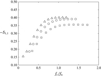
Difficulties in measuring quantities associated with the SSM have been discussed by a number of authors (e.g. Tennekes & Wyngaard Reference Tennekes and Wyngaard1972; Champagne Reference Champagne1978; Antonia, Satyaprakash & Hussain Reference Antonia, Satyaprakash and Hussain1982; Antonia, Anselmet & Chambers Reference Antonia, Anselmet and Chambers1986). Therefore, it is important to check the accuracy of the present measurements before discussing the results. Figure 1 shows the dependence of
 $-S_{1,1}$
on
 $f_{c}/f_{{\it\eta}}$
(
 $f_{c}$
is the cutoff frequency) at several Reynolds numbers. A forward differencing scheme was used to calculate
 $-S_{1,1}$
. The figure indicates that the magnitude of
 $S_{1,1}$
increases with
 $f_{c}/f_{{\it\eta}}$
, reaches a maximum at
 $f_{c}/f_{{\it\eta}}=1.0$
and remains constant at higher frequencies for all values of
 $h^{+}$
. A similar dependence was reported by Shah & Antonia (Reference Shah and Antonia1986). All the values of
 $-S_{1,1}$
shown in this paper have been estimated in a similar manner, i.e. by first plotting the dependence of
 $-S_{1,1}$
on
 $f_{c}/f_{{\it\eta}}$
using the forward differencing scheme before identifying the value of
 $-S_{1,1}$
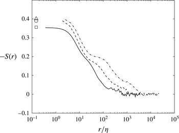
with that where a significant plateau occurs (see figure 1). The velocity increment skewness (
 $S(r)=\overline{({\rm\Delta}u_{1})^{3}}/\overline{({\rm\Delta}u_{1})^{2}}^{3/2}$
) is shown in figure 2 at the same
 $h^{+}$
as in figure 1. As expected, the magnitude of
 $S(r)$
tends to zero smoothly for large
 $r$
. When
 $r\rightarrow 0$
,
 $-S(r)$
tends, also as expected, to the same values of
 $-S_{1,1}$
as in figure 1. As
 $h^{+}$
increases, the distributions begin to exhibit a range where
 $-S(r)$
decreases only slowly with
 $r/{\it\eta}$
. According to K41,
 $-S(r)$
should approach a constant over this (inertial) range when
 $h^{+}\rightarrow \infty$
.
Dependence of
 $-S_{1,1}$
on
 $f_{c}/f_{{\it\eta}}$
on the channel centreline at three values of
 $h^{+}$
:
 $h^{+}=180$
, ▫;
 $h^{+}=582$
, ○;
 $h^{+}=1525$
, ▵.

Skewness structure function
 $-S(r)$
on the channel centreline at three values of
 $h^{+}$
:
 $h^{+}=180$
, solid curve;
 $h^{+}=582$
, dashed curve;
 $h^{+}=1525$
, dash-dotted curve. Symbols are values of
 $-S_{1,1}$
from figure 1 at the same
 $h^{+}$
.

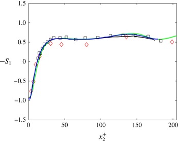
Figure 3 compares the skewness of the streamwise velocity fluctuation
 $u$
(denoted as
 $-S_{1}$
) in the
 $x_{2}^{+}$
direction with data from the literature. The unpublished data of Abe et al. (Reference Abe, Antonia and Kawamura2009) have been included. The agreement between the present distributions of
 $-S_{1}$
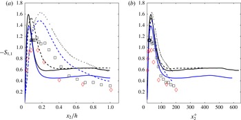
and those of both experimental and DNS data is satisfactory, especially in the outer region. However, the agreement for
 $-S_{1,1}$
between experimental and DNS data (figure 4) is relatively poor both in the wall and outer regions of the channel. Note that the level of agreement between the experimental data sets reflects that observed for
 $-S_{1}$
; both set of data agree relatively well in the outer region of the flow. On the other hand, for the DNS data of Abe et al. (Reference Abe, Antonia and Kawamura2009) and Vreman & Kuerten (Reference Vreman and Kuerten2014a
) at the same
 $h^{+}$
, the agreement is poor for
 $x_{2}^{+}\geqslant 20$
; the maximum values of
 $-S_{1,1}$
at
 $x_{2}^{+}=30$
is about 10 % greater for Abe et al. (Reference Abe, Antonia and Kawamura2009) than for Vreman & Kuerten (Reference Vreman and Kuerten2014a
); the two DNS distributions follow each other but remain offset by a constant amount, regardless of
 $h^{+}$
.
At the centreline, the present value of
 $-S_{1,1}$
is in good agreement with that of Vreman & Kuerten (Reference Vreman and Kuerten2014a
). For Abe et al. (Reference Abe, Antonia and Kawamura2009), the magnitude of
 $S_{1,1}$
increases with decreasing
 ${\rm\Delta}x_{1}$
and remains constant when
 ${\rm\Delta}x_{1}/{\it\eta}\leqslant 0.8$
(on the centreline). Vreman & Kuerten (Reference Vreman and Kuerten2014a
) also reported that the magnitude increases with decreasing
 ${\rm\Delta}x_{1}$
; however, their smaller
 ${\rm\Delta}x_{1}$
corresponds to
 ${\rm\Delta}x_{1}^{+}=4.42$
or
 ${\rm\Delta}x_{1}/{\it\eta}=1.2$
(on the centreline). This may explain, only in part, the differences between the two DNS distributions in figure 4. It does not, however, explain the difference between the present measured value of
 $-S_{1,1}$
and that of Abe et al. (Reference Abe, Antonia and Kawamura2009) since
 $l_{w}/{\it\eta}=0.5$
(on the centreline) for the present hot wire; also, the HIT simulations of Burattini, Lavoie & Antonia (Reference Burattini, Lavoie and Antonia2008) indicated that, for a single hot wire, the magnitude of
 $S_{1,1}$
is mainly affected by the temporal resolution and is practically insensitive to the spatial resolution. The preceding comments strongly suggest that the difference between the present measurement and the DNS values of
 $-S_{1,1}$
may be genuine. Similarly, the difference between the different DNS data for
 $-S_{1,1}$
may also be genuine.
Distributions of
 $-S_{1}$
at
 $h^{+}=180$
: ▫, present data; green curve, Kim et al. (Reference Kim, Moin and Moser1987); black curve, Abe et al. (Reference Abe, Antonia and Kawamura2009); blue curve, Vreman & Kuerten (Reference Vreman and Kuerten2014a
), ♢, Wallace, Brodkey & Eckelmann (Reference Wallace, Brodkey and Eckelmann1977) at
 $h^{+}=195$
.

Distributions of
 $-S_{1,1}$
: ▫, present data; dotted, dashed, and solid curves in black correspond to the simulation of Abe et al. (Reference Abe, Antonia and Kawamura2009) at
 $h^{+}=180$
, 395, and 640 respectively; dashed and solid curves in blue correspond to the simulation of Vreman & Kuerten (Reference Vreman and Kuerten2014a
,Reference Vreman and Kuerten
b
) at
 $h^{+}=180$
and 590 respectively; ♢, Wallace et al. (Reference Wallace, Brodkey and Eckelmann1977) at
 $h^{+}=195$
.

4.2. Approach to local isotropy at the centreline
Equations (1.6) and (2.9) are based on the assumption of local isotropy (LI). As noted in the Introduction, a significant departure from LI has been observed and documented in the literature for various statistics of both velocity and scalar derivative fields in a channel flow, although the departure tends to become smaller as the distance from the wall increases and, for fixed values of
 $x_{2}/h$
in the outer region, as
 $h^{+}$
increases. Here, we focus on the departure from LI in the specific context of (2.9). Using the isotropic form of a single-point sixth-order velocity derivative tensor
 $\overline{u_{i,j}u_{k,l}u_{m,n}}$
(Wyngaard Reference Wyngaard2010; Champagne Reference Champagne1978), it is easy to show that
 $$\begin{eqnarray}\overline{u_{1,1}^{3}}=\overline{u_{2,2}^{3}}=\overline{u_{3,3}^{3}}.\end{eqnarray}$$
The isotropic form of the forth-order velocity derivative tensor (Wyngaard Reference Wyngaard2010) leads to
 $$\begin{eqnarray}\overline{u_{1,1}^{2}}=\overline{u_{2,2}^{2}}=\overline{u_{3,3}^{2}}.\end{eqnarray}$$
It follows from (4.1) and (4.2) that
 $$\begin{eqnarray}S_{1,1}=S_{2,2}=S_{3,3}.\end{eqnarray}$$
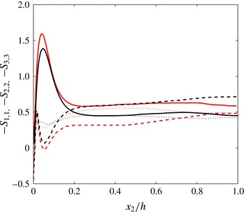
Figure 5 compares the distributions of
 $S_{1,1}$
,
 $S_{2,2}$
and
 $S_{3,3}$
from Vreman & Kuerten (Reference Vreman and Kuerten2014b
) at
 $h^{+}=590$
with those from Abe et al. (Reference Abe, Antonia and Kawamura2009) at
 $h^{+}=640$
. In the outer part of the channel, all distributions exhibit a region where the magnitude of the derivative skewness is approximately constant; this is more accentuated for
 $S_{1,1}$
than either
 $S_{2,2}$
or
 $S_{3,3}$
. There are, however, differences between Vreman & Kuerten (Reference Vreman and Kuerten2014b
) and Abe et al. (Reference Abe, Antonia and Kawamura2009). In each case, (4.3) is not obeyed, not even on the centreline. For Vreman & Kuerten (Reference Vreman and Kuerten2014b
),
 $S_{1,1}\approx S_{3,3}$
, the magnitude of
 $S_{2,2}$
being larger than that of either
 $S_{1,1}$
or
 $S_{3,3}$
. For Abe et al. (Reference Abe, Antonia and Kawamura2009),
 $S_{2,2}\approx S_{3,3}$
(
 ${<}S_{1,1}$
) at
 $x_{2}/h=1$
.
Distributions of
 $-S_{1,1}$
(solid),
 $-S_{2,2}$
(dashed), and
 $-S_{3,3}$
(dotted). Black and red curves correspond to Vreman & Kuerten (Reference Vreman and Kuerten2014b
) at
 $h^{+}=590$
and unpublished data of Abe et al. (Reference Abe, Antonia and Kawamura2009) at
 $h^{+}=640$
respectively.

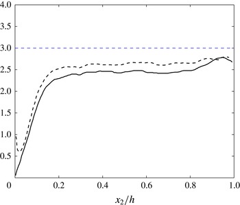
Distributions of the ratios
 $\overline{u_{2,11}^{2}}/\overline{u_{1,11}^{2}}$
(solid) and
 $\overline{u_{3,11}^{2}}/\overline{u_{1,11}^{2}}$
(dashed) at
 $h^{+}=640$
(unpublished data of Abe et al.
Reference Abe, Antonia and Kawamura2009). The horizontal line indicates the isotropic value of 3.

Wyngaard’s isotropic expression for
 $\overline{u_{i,km}u_{j,ln}}$
leads to
 $$\begin{eqnarray}\overline{u_{2,11}^{2}}=\overline{u_{3,11}^{2}}=3\overline{u_{1,11}^{2}}.\end{eqnarray}$$
The data of Abe et al. (Reference Abe, Antonia and Kawamura2009) (
 $h^{+}=640$
) indicate (figure 6) that the ratios
 $\overline{u_{2,11}^{2}}/\overline{u_{1,11}^{2}}$
and
 $\overline{u_{3,11}^{2}}/\overline{u_{1,11}^{2}}$
increase relatively slowly over the outer region but do not quite reach the isotropic value of 3 at the centreline. The ratios
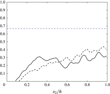
 $\overline{u_{1,1}u_{2,1}^{2}}/\overline{u_{1,11}^{3}}$
and
 $\overline{u_{1,1}u_{3,1}^{2}}/\overline{u_{1,11}^{3}}$
(figure 7), which also increase slowly in the outer region of the channel, indicate a bigger departure from isotropy (
 $=2/3$
) than the second-derivative ratios. Possibly, this may be due to the fact that the enstrophy production receives contributions from larger scales than the enstrophy dissipation. Indeed, the cospectrum between
 $u_{1,1}$
and
 $u_{1,1}^{2}$
peaks at
 $k_{1}^{\ast }\approx 0.06$
, whereas
 $k_{1}^{\ast 4}{\it\phi}_{u1}^{\ast }(k_{1}^{\ast })$
has a maximum at
 $k_{1}^{\ast }\approx 0.34$
(
 $k_{1}$
is the wavenumber,
 ${\it\phi}_{u1}$
is the one-dimentional spectrum and the asterisk denotes normalization by the Kolmogorov scales). Interestingly, if
 $\overline{u_{1,1}^{3}}=-2{\it\nu}\overline{u_{1,11}^{2}}$
, i.e. the result expected when the Reynolds number is sufficiently large and presumably when LI holds, then
 $\overline{u_{1,1}u_{i,1}^{2}}=(7/3)\overline{u_{1,1}^{3}}=-(14/3){\it\nu}\overline{u_{1,11}^{2}}$
and
 $\overline{u_{i,11}^{2}}=7\overline{u_{1,11}^{2}}$
, so that
 $$\begin{eqnarray}\frac{\overline{u_{1,1}u_{i,1}^{2}}}{{\it\nu}\overline{u_{i,11}^{2}}}=-\frac{2}{3}.\end{eqnarray}$$
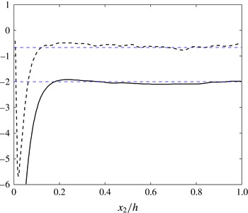
Figure 8 shows that (4.5) is actually verified at the centreline as well as
 $\overline{u_{1,1}^{3}}/{\it\nu}\overline{u_{1,11}^{2}}=-2$
, notwithstanding the departures from isotropy exhibited in figures 6 and 7.
Although individual components of the sixth-order velocity derivative tensors
 $\overline{u_{i,j}u_{k,l}u_{m,n}}$
and
 $\overline{u_{i,km}u_{j,ln}}$
exhibit departures from LI, there are, as in the case of the components of the fourth-order velocity derivative tensor, sufficient compensations to assume that, at least on the centreline, the vorticity budget satisfies isotropy reasonably well.
Distributions of the ratios
 $\overline{u_{1,1}u_{2,1}^{2}}/\overline{u_{1,11}^{3}}$
(solid) and
 $\overline{u_{1,1}u_{3,1}^{2}}/\overline{u_{1,11}^{3}}$
(dashed) at
 $h^{+}=640$
(unpublished data of Abe et al.
Reference Abe, Antonia and Kawamura2009). The horizontal line indicates the isotropic value of
 $2/3$
.

Distributions of the ratios
 $\overline{u_{1,1}^{3}}/{\it\nu}\overline{u_{1,11}^{2}}$
(solid) and
 $\overline{u_{1,1}u_{i,1}^{2}}/{\it\nu}\overline{u_{i,11}^{2}}$
(dashed) at
 $h^{+}=640$
(unpublished data of Abe et al.
Reference Abe, Antonia and Kawamura2009). The horizontal lines indicate the isotropic values of
 $-2/3$
and
 $-2$
respectively.

4.3. Calculation of
$G$

When estimating
 $G$
, a uniform treatment was applied to the measured distributions of
 ${\it\phi}_{u1}^{\ast }(k_{1}^{\ast })$
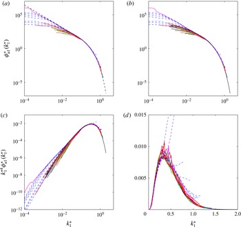
, primarily to avoid the effects of noise contamination and possible inadequate spatial resolution of the hot wires. The measured spectrum beyond
 $k_{1}^{\ast }\approx 0.3$
was ignored and a suitable fit was applied to the upper end of the scaling (inertial) range and lower end of the dissipation range before extrapolating it to a value of
 $k_{1}^{\ast }$
, typically between 1 and 2. The main rationale for using a universal extrapolation can be found in Antonia, Djenidi & Danaila (Reference Antonia, Djenidi and Danaila2014) who pointed out that the collapse of the turbulent dissipative range on Kolmogorov scales does not require either of the two major assumptions in K41, viz.
 $R_{{\it\lambda}}$
should be very large and local isotropy must be valid. Antonia et al. (Reference Antonia, Djenidi and Danaila2014) showed that a similarity solution of the SSM based on the Kolmogorov scales remains plausible provided the large-scale inhomogeneity in the Kelvin–Helmholtz equation is small with respect to the term containing
 $\overline{{\it\epsilon}}$
and
 ${\it\nu}$
. Kolmogorov normalization breaks down only when
 $R_{{\it\lambda}}$
falls below a value of about 20 (Djenidi et al.
Reference Djenidi, Tardu, Antonia and Danaila2014). The robustness of the collapse of
 ${\it\phi}_{u1}^{\ast }(k_{1}^{\ast })$
at sufficiently large
 $k_{1}^{\ast }$
underpins the extrapolation used here to estimated
 $G$
. Several approaches could have been adopted for carrying out the extrapolation. Here we used the model spectrum of Pope (Reference Pope2000)
 $$\begin{eqnarray}{\it\phi}(k)=C\,\overline{{\it\epsilon}}^{2/3}k_{1}^{-5/3}\,f_{{\it\eta}},\end{eqnarray}$$
with
 $f_{{\it\eta}}=\exp \{-{\it\beta}\{[(k_{1}{\it\eta})^{4}+c_{{\it\eta}}^{4}]^{1/4}-c_{{\it\eta}}\}\}$
. For Pope, the constants are
 $c_{{\it\eta}}\approx 0.40$
,
 $C=1.5$
, and
 ${\it\beta}=5.2$
. We have used
 $c_{{\it\eta}}=0.11$
,
 $C=0.6$
and
 ${\it\beta}=7.2$
. Note that, in its original form, Pope’s expression contains the term
 $f_{L}(k_{1}L)$
, which determines the shape of the energy-containing range (i.e. low
 $k_{1}L$
) and tends to unity for large
 $k_{1}L$
. Since the focus of the present extrapolation is on the high-wavenumber range of the spectrum that term is set to one. It is important to stress that the very good collapse of the data in the range of interest (i.e.
 $k_{1}{\it\eta}\geqslant 0.1$
see figure 9
a) implies that the model spectrum ((4.6) with the new coefficients) represents a curve fit to all the spectra shown in figure 9(a). Clearly, one could use, for example, the well-resolved DNS spectrum on the centreline of a channel flow, for which a
 $k^{-5/3}$
region is not observed, to extrapolate the measured spectra. There is now ample experimental, numerical and theoretical evidence that this part of the spectrum is universal (Antonia et al.
Reference Antonia, Djenidi and Danaila2014). Equally, any number of sufficiently well-resolved experimental spectra (see for example Antonia et al.
Reference Antonia, Djenidi and Danaila2014) could have been used for this purpose. We stress here that the use of
 $k_{1}^{-5/3}$
in (4.6) has not biased the values of
 $G/R_{{\it\lambda}}$
that have been estimated from the extrapolated spectra.
Normalized one-dimensional longitudinal velocity spectra and its fourth moments. (a) One-dimensional longitudinal velocity spectra: red curves (experimental and DNS data) were compiled in Antonia et al. (Reference Antonia, Djenidi and Danaila2014); pink curve, Larssen & Devenport (Reference Larssen and Devenport2011); green curves, Abe et al. (Reference Abe, Antonia and Kawamura2009); blue curves, Moser, Kim & Mansour (Reference Moser, Kim and Mansour1999); blue dashed curves, Rosenberg et al. (Reference Rosenberg, Hultmark, Vallikivi, Bailey and Smits2013); black dashed curve is the calculated one-dimensional longitudinal velocity spectra with the model spectrum of Pope (Reference Pope2000). (b) Comparison of the extrapolated spectra in the present channel flow (black curve) with the spectra in (a), (c,d)
 $k_{1}^{\ast 4}{\it\phi}_{u1}^{\ast }(k_{1}^{\ast })$
corresponding to the spectra in (b) in logarithmic and linear coordinates respectively.

Figure 9(b) shows the extrapolated spectra in the present channel flow (the extrapolation extends to values of
 $k_{1}^{\ast }$
that are just slightly larger than 2), and for comparison, the spectra in figure 9(a) are also included. As expected, the present extrapolated spectra collapse well with all other spectra considered here in the dissipative range, in accordance with Kolmogorov scaling. Figure 9(c,d) shows that the distributions of
 $k_{1}^{\ast 4}{\it\phi}_{u1}^{\ast }(k_{1}^{\ast })$
correspond to figure 9(b) in both the linear and logarithmic coordinates. Also as expected, there is a relatively good collapse of the spectra in the dissipative ranges, despite the scatter at
 $k_{1}{\it\eta}\approx 0.38$
in figure 9(d) (this scatter is mainly due to the uncertainty of our digitization). Note that in figure 9(b–d), the poor agreement between the present spectra and those of Rosenberg et al. (Reference Rosenberg, Hultmark, Vallikivi, Bailey and Smits2013) (blue dashed curve) is likely to have been caused by the insufficient spatial resolution in their measurements. The term
 $G$
, defined by (1.4), can be rewritten as
 $$\begin{eqnarray}G=\frac{\overline{u_{1}^{\ast 2}}\overline{\left(\partial ^{2}u_{1}^{\ast }/\partial x_{1}^{\ast 2}\right)^{2}}}{\overline{\left(\partial u_{1}^{\ast }/\partial x_{1}^{\ast }\right)^{2}}^{2}},\end{eqnarray}$$
If local isotropy holds, so that
 $\overline{{\it\epsilon}}=\overline{{\it\epsilon}}_{iso}=15{\it\nu}\overline{(\partial u_{1}/\partial x_{1})^{2}}$
, (4.7) can be rewritten as
 $$\begin{eqnarray}\frac{2G}{R_{{\it\lambda}}}=2\times 15^{3/2}\int _{0}^{\infty }{k_{1}^{\ast }}^{4}{\it\phi}_{u1}^{\ast }(k_{1}^{\ast })\,\text{d}k_{1}^{\ast },\end{eqnarray}$$
where
 ${\it\phi}_{u1}^{\ast }(k_{1}^{\ast })$
is the one-dimensional spectral density of
 $u_{1}$
, defined such that
 $\int _{0}^{\infty }{\it\phi}_{u1}(k_{1})\,\text{d}k_{1}=\overline{u_{1}^{2}}$
. If there is a small departure from local isotropy, then
 $2G/R_{{\it\lambda}}$
is estimated using
 $$\begin{eqnarray}\frac{2G}{R_{{\it\lambda}}}=2{\it\nu}\frac{\displaystyle \int _{0}^{\infty }k_{1}^{4}{\it\phi}_{u1}(k_{1})\,\text{d}k_{1}}{\left[\displaystyle \int _{0}^{\infty }k_{1}^{2}{\it\phi}_{u1}(k_{1})\,\text{d}k_{1}\right]^{3/2}}.\end{eqnarray}$$
Since, as seen earlier, there are small departures from local isotropy along the channel centreline, in this paper we estimate
 $2G/R_{{\it\lambda}}$
from (4.9) after extrapolation of
 ${\it\phi}_{u1}^{\ast }(k_{1}^{\ast })$
(figure 9
b).
5. Results
5.1. Validation of equation (2.9)
Here, we test (2.9) against measurements at
 $h^{+}=180$
. A perfect validation of (2.9) requires that the diffusion term (left-hand side) balances the sum
 $S_{1,1}+2G/R_{{\it\lambda}}$
exactly. On the centreline of the channel, it can be seen from figure 1 that
 $-S_{1,1}$
is about 0.36. Following the procedure shown in the above section, we estimate that
 $2G/R_{{\it\lambda}}$
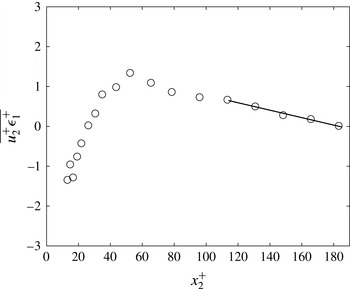
is about 0.60 at this location. Figure 10 shows the distribution of
 $\overline{u_{2}^{+}{\it\epsilon}_{1}^{+}}$
, with respect to
 $x_{2}^{+}$
, obtained with the one-component vorticity probe, where three different measurements of
 $u_{1}$
are made simultaneously with
 $u_{2}$
at each
 $x_{2}$
location. Each point shown in figure 10 is an average of the three values. The magnitude of
 $\overline{u_{2}^{+}{\it\epsilon}_{1}^{+}}$
increases rapidly in the inner layer, reaching a maximum at about
 $x_{2}^{+}=50$
, and then decreases slowly farther away from the wall before approaching zero on the centreline of the channel. The term on the left-hand side of (2.9) is obtained by applying a least-squares linear fit to the distribution of
 $\overline{u_{2}^{+}{\it\epsilon}_{1}^{+}}$
over the range
 $x_{2}^{+}=110{-}180$
, and then normalizing the slope of the fitted line with
 $\overline{{\it\epsilon}}_{iso}$
on the channel centreline and
 ${\it\nu}$
. Its magnitude is thus found to be equal to 0.25, as shown in table 1, where estimates of
 $S_{1,1}$
,
 $2G/R_{{\it\lambda}}$
, and
 $S_{1,1}+2G/R_{{\it\lambda}}$
are also included. The conclusion we draw from this table is that (2.9) is satisfied adequately on the centreline of the channel.
Distribution of
 $\overline{u_{2}^{+}{\it\epsilon}_{1}^{+}}$
in the
 $x_{2}^{+}$
direction at
 $h^{+}=180$
. Solid line is a linear fit over the range
 $x_{2}^{+}=110{-}180$
.

Check of equation (2.9) at
 $h^{+}=180$
using data from a one-component vorticity probe.

The vorticity budget is given by (Abe et al. Reference Abe, Antonia and Kawamura2009)
 $$\begin{eqnarray}\underbrace{-0.5\frac{\partial }{\partial y}\overline{v{\it\omega}_{i}{\it\omega}_{i}}}_{\mathit{Diffusion}\equiv \mathit{Dif}}+\underbrace{\overline{{\it\omega}_{i}{\it\omega}_{j}\unicode[STIX]{x1D634}_{ij}}+\overline{{\it\omega}_{i}{\it\omega}_{j}\unicode[STIX]{x1D61A}_{ij}}+\bar{{\it\omega}}_{j}\overline{{\it\omega}_{i}\unicode[STIX]{x1D634}_{ij}}}_{\mathit{Production}\equiv \mathit{P}}-\underbrace{{\it\nu}\overline{{\it\omega}_{i}{\it\omega}_{i}}}_{\mathit{Dissipation}\equiv \mathit{D}}=0,\end{eqnarray}$$
where the mean strain rate
 $\unicode[STIX]{x1D61A}_{ij}$
and the strain-rate fluctuations
 $\unicode[STIX]{x1D634}_{ij}$
are given by
 $$\begin{eqnarray}\unicode[STIX]{x1D61A}_{ij}\equiv \left\{\begin{array}{@{}l@{}}\displaystyle \frac{1}{2}\left(\displaystyle \frac{\partial U_{i}}{\partial x_{j}}+\displaystyle \frac{\partial U_{j}}{\partial x_{i}}\right)\quad \\ \displaystyle \frac{1}{2}\left(\displaystyle \frac{\partial u_{i}}{\partial x_{j}}+\displaystyle \frac{\partial u_{j}}{\partial x_{i}}\right).\quad \end{array}\right.\end{eqnarray}$$
The DNS vorticity budget data (Antonia & Kim Reference Antonia and Kim1994) at
 $h^{+}=180$
and 395 and (Abe et al.
Reference Abe, Antonia and Kawamura2009) at
 $h^{+}=180$
, 395 and 640 have been used to assess the magnitude of the ratios
 $Dif/D$
and
 $P/D$
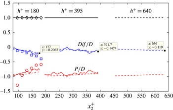
in the outer part of the channel. In figure 11, the ratios shown up to
 $x_{2}^{+}\simeq 180$
are for
 $h^{+}=180$
. For
 $200\leqslant x_{2}^{+}\leqslant 400$
, the ratios are for
 $h^{+}=395$
; and for
 $x_{2}^{+}\geqslant 450$
, the ratios are for
 $h^{+}=640$
. For both DNS data sets at
 $h^{+}=180$
, there is a tendency for
 $|Dif/D|$
to increase and
 $|P/D|$
to decrease as the centreline is approached; this is more marked for the experimental data than for the DNS data. At the centreline,
 $|Dif/D|\simeq 0.21$
for the DNS data of Abe et al. (Reference Abe, Antonia and Kawamura2009) compared to 0.40 for the experiment (
 $|Dif/D|\simeq 0.25$
for Antonia & Kim Reference Antonia and Kim1994). For
 $h^{+}=395$
, the variation with
 $x_{2}^{+}$
is small in the outer region, and
 $|Dif/D|$
is only 0.15 at the centreline for both DNS data sets.
 $|Dif/D|$
becomes even smaller at
 $h^{+}=640$
(
 $|Dif/D|=0.12$
on the centreline). In contrast,
 $|P/D|$
contributes significantly to the vorticity budget with increasing
 $h^{+}$
. Figure 11 shows a decreasing trend for
 $|Dif/D|$
with increasing
 $h^{+}$
. This is consistent with, at sufficiently high Reynolds number,
 $|Dif/D|$
becoming negligible, i.e.
 $|P/D|\approx 1$
. The same should be true for the isotropic budget (2.9) and will be addressed in § 5.2.
Vorticity budget of DNS data (Antonia & Kim Reference Antonia and Kim1994) at
 $h^{+}=180$
and 395 (solid curves) and (Abe et al.
Reference Abe, Antonia and Kawamura2009) at
 $h^{+}=180$
, 395 and 640 (dashed curves) in the outer layer. Note that each term is normalized by the dissipation term; three tagged points are the ratios
 $Dif/D$
at the channel centreline for Abe et al. (Reference Abe, Antonia and Kawamura2009). Symbols are the isotropic budget (2.9) of experimental data at
 $h^{+}=180$
: ▫, diffusion term; ○, production term (
 $S_{1,1}$
); ♢, dissipation term (
 $2G/R_{{\it\lambda}}$
); note that each is divided by the dissipation term.

5.2. Scaling of the transport equation
After applying dimensional arguments to the kinetic energy production term, Bernardini, Pirozolli & Orlandi (Reference Bernardini, Pirozolli and Orlandi2014) argued that, for the region close the centreline of the channel, while
 $v^{\prime }$
,
 $w^{\prime }$
and
 $u^{\prime }v^{\prime }$
scale with
 $U_{{\it\tau}}$
,
 $u^{\prime }$
scales with
 $\sqrt{U_{{\it\tau}}U_{cl}}$
. Here we extend their argument to the transport equation for
 $\overline{{\it\epsilon}}_{iso}$
along the channel centreline. Since the turbulent kinetic energy production term
 $P$
should scale as
 $P\sim U_{{\it\tau}}^{2}U_{cl}/h$
,
 $\overline{{\it\epsilon}}_{iso}$
should thus have the same scaling as
 $P$
,
 $$\begin{eqnarray}\overline{{\it\epsilon}}_{iso}\sim P\sim U_{{\it\tau}}^{2}U_{cl}/h.\end{eqnarray}$$
The diffusion of
 ${\it\epsilon}_{1}$
by
 $u_{2}$
should scale as
 $$\begin{eqnarray}\frac{\partial \overline{u_{2}{\it\epsilon}_{1}}}{\partial x_{2}}\sim \overline{{\it\epsilon}}_{iso}/{\it\tau},\end{eqnarray}$$
where
 ${\it\tau}=h/U_{{\it\tau}}$
is the typical eddy turnover time in the outer region of the channel (Jimenez, Hoyas & Mizuno Reference Jimenez, Hoyas and Mizuno2009). Hence, it follows that
 $$\begin{eqnarray}\frac{\partial \overline{u_{2}{\it\epsilon}_{1}}}{\partial x_{2}}\sim U_{{\it\tau}}^{3}U_{cl}/h^{2}.\end{eqnarray}$$
The term on the left of (2.9) can therefore be rewritten as follows:
 $$\begin{eqnarray}\displaystyle & & \displaystyle -\displaystyle \frac{3}{7{\it\nu}}\displaystyle \frac{\partial \overline{u_{2}{\it\epsilon}_{1}}}{\partial x_{2}}\bigg/\left(\displaystyle \frac{\overline{{\it\epsilon}}^{3/2}}{(15{\it\nu})^{3/2}}\right)=-\displaystyle \frac{45\sqrt{15}}{7}\displaystyle \frac{\partial \overline{u_{2}{\it\epsilon}_{1}}}{\partial x_{2}}\displaystyle \frac{{\it\nu}^{1/2}}{\overline{{\it\epsilon}}^{3/2}}=-\displaystyle \frac{45\sqrt{15}}{7}\displaystyle \frac{\partial \overline{\displaystyle \frac{u_{2}{\it\epsilon}_{1}h}{U_{{\it\tau}}^{3}U_{cl}}}}{\partial \displaystyle \frac{x_{2}}{h}}\displaystyle \frac{\left(\displaystyle \frac{{\it\nu}}{U_{cl}h}\right)^{1/2}}{\overline{\left(\displaystyle \frac{{\it\epsilon}h}{U_{{\it\tau}}^{2}U_{cl}}\right)}^{3/2}}\nonumber\\ \displaystyle & & \displaystyle \quad =-\displaystyle \frac{45\sqrt{15}}{7}\displaystyle \frac{\partial \overline{\displaystyle \frac{u_{2}{\it\epsilon}_{1}h}{U_{{\it\tau}}^{3}U_{cl}}}}{\overline{\left(\displaystyle \frac{{\it\epsilon}h}{U_{{\it\tau}}^{2}U_{cl}}\right)}^{3/2}\partial \displaystyle \frac{x_{2}}{h}}\displaystyle \frac{1}{(R_{cl})^{1/2}}=-\displaystyle \frac{45\sqrt{15}}{7}\displaystyle \frac{\partial \overline{\displaystyle \frac{u_{2}{\it\epsilon}_{1}h}{U_{{\it\tau}}^{3}U_{cl}}}}{\overline{\left(\displaystyle \frac{{\it\epsilon}h}{U_{{\it\tau}}^{2}U_{cl}}\right)}^{3/2}\partial \displaystyle \frac{x_{2}}{h}}\displaystyle \frac{C_{1}}{R_{{\it\lambda}}}=C\displaystyle \frac{1}{R_{{\it\lambda}}},\nonumber\\ \displaystyle & & \displaystyle\end{eqnarray}$$
where
 $$\begin{eqnarray}R_{cl}=\displaystyle \frac{U_{cl}h}{{\it\nu}},\quad \displaystyle \frac{R_{{\it\lambda}}}{(R_{cl})^{1/2}}=C_{1},\quad \text{and}\quad C=-\displaystyle \frac{45\sqrt{15}C_{1}}{7}\displaystyle \frac{\partial \overline{\displaystyle \frac{u_{2}{\it\epsilon}_{1}h}{U_{{\it\tau}}^{3}U_{cl}}}}{\overline{\left(\displaystyle \frac{{\it\epsilon}h}{U_{{\it\tau}}^{2}U_{cl}}\right)}^{3/2}\partial \displaystyle \frac{x_{2}}{h}}.\end{eqnarray}$$
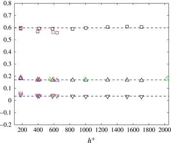
Figure 12 confirms the Reynolds number independence of
 $C_{1}$
as well as of the ratios
 $\sqrt{\overline{u^{2}}/(U_{{\it\tau}}U_{cl})}$
and
 $\overline{{\it\epsilon}}_{iso}h/(U_{{\it\tau}}^{2}U_{cl})$
, thus indicating that (5.6) is reasonably well supported by the present experimental data. Therefore, (2.9) can be rewritten in the form
 $$\begin{eqnarray}S_{1,1}+2\frac{G}{R_{{\it\lambda}}}=C\frac{1}{R_{{\it\lambda}}},\end{eqnarray}$$
where
 $C\,({\approx}9.7)$
estimated at
 $h^{+}=180$
should be independent of
 $R_{{\it\lambda}}$
. Arguably, the first term in (2.9) approaches zero at sufficiently large
 $R_{{\it\lambda}}$
. This is consistent with
 $C/R_{{\it\lambda}}$
approaching zero at infinite
 $R_{{\it\lambda}}(\lim _{R_{{\it\lambda}}\rightarrow \infty }(C/R_{{\it\lambda}})=0)$
. The main objective in deriving (5.7) is to assess the way
 $S_{1,1}+2G/R_{{\it\lambda}}$
approaches zero along the centreline of a fully developed channel flow as
 $R_{{\it\lambda}}$
increases and compare it with how
 $S_{1,1}+2G/R_{{\it\lambda}}$
approaches zero in other flows, e.g. decaying HIT, the axis of a turbulent round jet, and SFPBT.
Variation of
 $C_{1}$
with
 $h^{+}$
on the channel centreline (▫);
 $\sqrt{\overline{u^{2}}/(U_{{\it\tau}}U_{cl})}$
(▵); and the normalized dissipation rate
 $\overline{{\it\epsilon}}_{iso}h/(U_{{\it\tau}}^{2}U_{cl})$
(▿). Black symbols, present data; red, Moser et al. (Reference Moser, Kim and Mansour1999); blue, Abe et al. (Reference Abe, Antonia and Kawamura2009); green, Bernardini et al. (Reference Bernardini, Pirozolli and Orlandi2014); the horizontal lines indicate the mean values of the present data.

The statement that
 $S_{1,1}+2G/R_{{\it\lambda}}$
approaches zero as the Reynolds number increases may be obtained via several different arguments.
We first consider that (5.4) applies, with
 ${\it\tau}$
the characteristic time of the turbulent diffusion of
 ${\it\epsilon}_{1}$
along
 $x_{2}$
. Therefore, the left-hand side of (2.9) (hereafter denoted
 $LSE$
) scales as
 $$\begin{eqnarray}LSE=\frac{1}{{\it\nu}}\frac{\overline{{\it\epsilon}}}{{\it\tau}}\bigg/\frac{\overline{{\it\epsilon}}^{3/2}}{{\it\nu}^{3/2}}\sim \frac{{\it\nu}^{1/2}}{\overline{{\it\epsilon}}^{1/2}{\it\tau}}.\end{eqnarray}$$
Together with
 ${\it\tau}\sim \mathscr{L}\big/\mathscr{U}$
(where
 $\mathscr{L}$
and
 $\mathscr{U}$
are the length and velocity scales) and the normalized energy dissipation rate
 $$\begin{eqnarray}C_{{\it\epsilon}}\equiv \frac{\overline{{\it\epsilon}}\mathscr{L}}{\mathscr{U}^{3}},\end{eqnarray}$$
 $LSE$
becomes, after some straightforward calculations
 $$\begin{eqnarray}LSE=\frac{1}{C_{{\it\epsilon}}^{1/2}}\left(\frac{{\it\nu}}{\mathscr{U}\mathscr{L}}\right)^{1/2}=C_{{\it\epsilon}}^{-1/2}Re_{\mathscr{ L}}^{-1/2}.\end{eqnarray}$$
Since
 $C_{{\it\epsilon}}$
tends to a constant (which may depend on IBC) for
 $R_{{\it\lambda}}\geqslant 100$
(e.g. Abe & Antonia Reference Abe and Antonia2011), then
 $LSE\rightarrow 0$
as
 $Re_{\mathscr{L}}$
increases. If
 $\mathscr{L}$
is the integral scale of the flow, then
 $R_{{\it\lambda}}\sim Re_{\mathscr{L}}^{1/2}$
and the right-hand side of (5.7) is retrieved.
A similar development should hold for any other flow, with the restriction that local isotropy holds. The particular path along which
 $C_{{\it\epsilon}}$
tends to a constant is, again, flow specific, but it is commonly accepted that a constant value (though IBC dependent) is reached for sufficiently high Reynolds numbers (see for example Sreenivasan Reference Sreenivasan1998; Burattini, Lavoie & Antonia Reference Burattini, Lavoie and Antonia2005; Vassilicos Reference Vassilicos2015). In the near-field region downstream of the fractal grids as well as regular grids,
 $C_{{\it\epsilon}}$
is not constant with
 $x$
but may be approximated by a ratio
 $Re_{I}/Re_{\mathscr{L}}$
, where
 $Re_{I}$
is a global/inlet Reynolds number (see for example Valente & Vassilicos Reference Valente and Vassilicos2012; Hearst & Lavoie Reference Hearst and Lavoie2014; Vassilicos Reference Vassilicos2015). In this case, (5.10) would lead to
 $LSE\sim Re_{I}^{-1/2}$
rather than
 $LSE\sim R_{{\it\lambda}}^{-1}$
, as indicated by (5.7). In the far field of an axisymmetric jet, included in figures 14 and 15,
 $R_{{\it\lambda}}$
is constant along the axis. This region of the flow is exactly self-preserving and
 $C_{{\it\epsilon}}$
like
 $R_{{\it\lambda}}$
is constant with respect to
 $x$
.
A different way to reach the same outcome is to explicitly suppose self-preservation of the functions involved in
 $LSE$
, viz.
 $$\begin{eqnarray}\overline{v{\it\epsilon}}\sim \frac{\mathscr{U}^{4}}{\mathscr{L}}f_{v{\it\epsilon}}(x_{2}/\mathscr{L}),\end{eqnarray}$$
and
 $$\begin{eqnarray}\overline{{\it\epsilon}}=\frac{\mathscr{U}^{3}}{\mathscr{L}}f_{{\it\epsilon}}(x_{2}/\mathscr{L}),\end{eqnarray}$$
where
 $f_{v{\it\epsilon}}$
and
 $f_{{\it\epsilon}}$
are self-preserving functions which may depend on IBC. It follows that
 $LSE$
scales as
 $Re_{\mathscr{L}}^{-1/2}$
. This demonstration circumvents the explicit dependence on
 $C_{{\it\epsilon}}$
, and requires self-preservation. Note that the latter assumption is, however, implicit when writing equation (5.4).
A more general viewpoint may be provided in flows characterized by large-scale production, e.g. shear flows. In this case, with the one-point energy budget being given by
 $\bar{{\it\epsilon}}=2\overline{uv}(\partial \overline{U}/\partial y)$
,
 $LSE$
can be written as
 $$\begin{eqnarray}LSE\simeq \displaystyle \frac{\overline{\displaystyle \frac{\partial u}{\partial x}\displaystyle \frac{\partial v}{\partial x}}\displaystyle \frac{\text{d}\overline{U}}{\text{d}y}}{\overline{uv}\displaystyle \frac{\text{d}\overline{U}}{\text{d}y}}\displaystyle \frac{{\it\nu}}{\overline{\left(\displaystyle \frac{\partial u}{\partial x}\right)^{2}}^{1/2}}.\end{eqnarray}$$
Now,
 $$\begin{eqnarray}\displaystyle \frac{\overline{\displaystyle \frac{\partial u}{\partial x}\displaystyle \frac{\partial v}{\partial x}}\displaystyle \frac{\text{d}\overline{U}}{\text{d}y}}{\overline{uv}\displaystyle \frac{\text{d}\overline{U}}{\text{d}y}}=\displaystyle \frac{\overline{\displaystyle \frac{\partial u}{\partial x}\displaystyle \frac{\partial v}{\partial x}}}{\overline{uv}}\simeq \displaystyle \frac{1}{{\it\lambda}^{2}},\end{eqnarray}$$
and (5.13) becomes
 $$\begin{eqnarray}LSE\simeq \frac{1}{{\it\lambda}^{2}}\frac{{\it\nu}{\it\lambda}}{u^{\prime }}=\frac{{\it\nu}}{{\it\lambda}u^{\prime }}=R_{{\it\lambda}}^{-1}.\end{eqnarray}$$
Similarly, any flow, either decaying or forced, may be tackled, with the same qualitative final result. The constants in front of term
 $R_{{\it\lambda}}^{-1}$
are flow and IBC dependent, as the precise form of
 $LSE$
changes from flow to flow.
We have thus reinforced the claim that
 $S_{1,1}+2G/R_{{\it\lambda}}$
tends to zero for sufficiently high Reynolds numbers (independently of the exact definition of the Reynolds number). Moreover, as already emphasized, because
 $G/R_{{\it\lambda}}$
becomes constant at
 $R_{{\it\lambda}}\simeq 70$
, then
 $S_{1,1}$
becomes constant for large Reynolds numbers, which is analogous to the normalized dissipation
 $C_{{\it\epsilon}}$
becoming constant at a sufficiently high Reynolds number.
Dependence of
 $2G/R_{{\it\lambda}}$
on
 $R_{{\it\lambda}}$
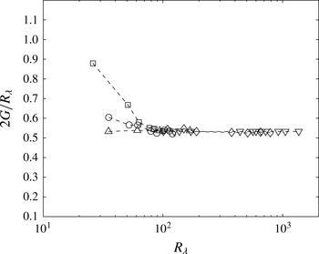
in different flows. Channel centreline: ○, present data; grid turbulence: ▫, Zhou & Antonia (Reference Zhou and Antonia2000) and ▿, Larssen & Devenport (Reference Larssen and Devenport2011); SFPBT: △, Jimenez et al. (Reference Jimenez, Wray, Saffman and Rogallo1993); pipe axis: ♢, Rosenberg et al. (Reference Rosenberg, Hultmark, Vallikivi, Bailey and Smits2013).

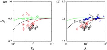
Dependence of
 $-S_{1,1}$
on
 $R_{{\it\lambda}}$
in different flows. (a) Channel centreline: ○, present data; ♢, Abe et al. (Reference Abe, Antonia and Kawamura2009); *, Vreman & Kuerten (Reference Vreman and Kuerten2014b
); pipe axis: ✩, Antonia & Pearson (Reference Antonia and Pearson2000a
); SFPBT: ▵, Jimenez et al. (Reference Jimenez, Wray, Saffman and Rogallo1993);
 $\times$
, Kerr (Reference Kerr1985); ▹, Wang et al. (Reference Wang, Chen, Brasseur and Wyngaard1996); green curve, Qian (Reference Qian1994); EDQNM simulation of decaying HIT: black curve, Meldi & Sagaut (Reference Meldi and Sagaut2013). Red curve is inferred from
 $S_{1,1}=C/R_{{\it\lambda}}-2G/R_{{\it\lambda}}$
by assuming
 $2G/R_{{\it\lambda}}=\text{constant}$
(
 ${\approx}0.52$
for
 $R_{{\it\lambda}}>70$
) on the channel centreline (similarly, the blue curve in (b) is inferred from the same equation along the jet axis). (b) Grid turbulence: ▫, Zhou & Antonia (Reference Zhou and Antonia2000); ○, Mydlarski & Warhaft (Reference Mydlarski and Warhaft1996); jet axis: ●, Mi, Xu & Zhou (Reference Mi, Xu and Zhou2013); ▪, Lefeuvre, Djenidi & Antonia (Reference Lefeuvre, Djenidi and Antonia2015); ▵, P. Burattini (private communication);
 $+$
, Kahalerras, Malecot & Gagne (Reference Kahalerras, Malecot and Gagne1998); ▿, Friehe et al. (Reference Friehe, Van Atta and Gibson1971). Some data in (a) are reproduced in (b) for the purpose of comparison.

5.3. Validation of equation (5.7)
Estimates of
 $2G/R_{{\it\lambda}}$
and
 $S_{1,1}$
for the present flow are shown in figures 13 and 14 by following the procedure outlined in § 4. Also included in figure 13 are estimates inferred from experimental and DNS data in other flows, such as SFPBT, along the axis of a pipe, and grid turbulence. As noted in the Introduction, there is abundant evidence to indicate that the ratio
 $G/R_{{\it\lambda}}$
approaches a constant relatively rapidly with increasing
 $R_{{\it\lambda}}$
, e.g. Lee et al. (Reference Lee, Djenidi, Antonia and Danaila2013). This is consistent with figure 13 which shows that, for all the flows considered here,
 $2G/R_{{\it\lambda}}$
is very nearly constant for
 $R_{{\it\lambda}}\geqslant 70$
. For
 $R_{{\it\lambda}}<70$
,
 $2G/R_{{\it\lambda}}$
appears to be flow dependent. For example, the approach to a constant value is slow in grid turbulence and rapid in SFPBT. For the present flow along the centreline of the channel, the approach is between grid turbulence and SFPBT. It should be noted that the constancy of
 $2G/R_{{\it\lambda}}$
is not an artefact of the extrapolation because the present extrapolated spectra collapse well with all other non-extrapolated spectra (see figure 9
d) in the dissipative range in accordance with Kolmogorov scaling. In his analysis, Champagne (Reference Champagne1978) used a ninth-order least-squares polynomial fit to extrapolate their spectrum and reported a value of 0.64 for
 $2G/R_{{\it\lambda}}$
(not shown in figure 13) on the centreline of the far field of a plane wake at
 $R_{{\it\lambda}}=182$
(
 $x/d=299$
). It is, however, likely that this polynomial fit strongly depends on the accuracy of the spectrum in the high-wavenumber range where the extrapolation is applied. The inadequacy of the spatial resolution (
 ${\it\eta}/l_{w}=0.81$
) tends to amplify the errors caused by the polynomial fit, thus yielding overestimated values of
 $2G/R_{{\it\lambda}}$
. Using either the spectral model of Pope (see § 4) or DNS spectra to extrapolate the spectrum of Champagne (Reference Champagne1978), we obtained a value of about 0.52, which is consistent with figure 13.
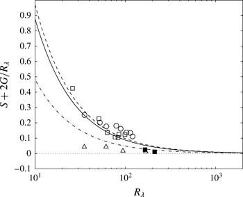
Dependence of
 $S_{1,1}+2G/R_{{\it\lambda}}$
on
 $R_{{\it\lambda}}$
in different flows. Symbols are the experimental and numerical data. Channel centreline: ○, present data; grid turbulence: ▫, Zhou & Antonia (Reference Zhou and Antonia2000); SFPBT: ▵, Jimenez et al. (Reference Jimenez, Wray, Saffman and Rogallo1993); jet axis: ▪, Lefeuvre et al. (Reference Lefeuvre, Djenidi and Antonia2015). The four curves (solid, dashed, dash-dotted and dotted curves), inferred from (5.7) (
 $C$
is flow dependent), correspond to grid turbulence, the centreline of a channel flow, the axis of a round jet, and SFPBT, respectively.

In contrast to figure 13, the distributions of
 $S_{1,1}$
(figure 14
a,b) exhibit significant differences between different flows. Figure 14(a) shows the data, both DNS and measurements, for
 $-S_{1,1}$
on the centreline of the channel flow as well as measurements on the centreline of a pipe, SFPBT and eddy-damped quasi-normal Markovian (EDQNM) results for decaying homogeneous and isotropic turbulence (Meldi & Sagaut Reference Meldi and Sagaut2013). Figure 14(b) compares
 $-S_{1,1}$
between the present measurements in the channel flow and measurements in other turbulent flows (e.g. grid turbulence and jet flows). As expected, the magnitude of
 $S_{1,1}$
is virtually constant in SFPBT; the value of 0.52 is in good agreement with the analytical prediction of Qian (Reference Qian1994). Along the axis of the jet flow, the magnitude of
 $S_{1,1}$
is somewhat smaller than that in SFPBT at small
 $R_{{\it\lambda}}$
but approaches quickly the value of 0.52 as
 $R_{{\it\lambda}}$
increases. The data shown include the measurements of Mi et al. (Reference Mi, Xu and Zhou2013), Lefeuvre et al. (Reference Lefeuvre, Djenidi and Antonia2015) with
 $d_{w}=1.24~{\rm\mu}\text{m}$
, P. Burattini (private communication), Friehe et al. (Reference Friehe, Van Atta and Gibson1971), and Kahalerras et al. (Reference Kahalerras, Malecot and Gagne1998). Except for Mi et al. (Reference Mi, Xu and Zhou2013), all the values of
 $-S_{1,1}$
were obtained by assuming that
 $\partial /\partial x=-(1/U_{c})(\partial /\partial t)$
, where
 $U_{c}\equiv U$
is the instantaneous velocity along
 $x$
. Kahalerras et al. (Reference Kahalerras, Malecot and Gagne1998) showed that this is preferable to the use of Taylor’s hypothesis (
 $U_{c}\equiv \overline{U}$
) which is inadequate when the local turbulence intensity is high (typically 25–30 %). The large value of
 $-S_{1,1}$
(0.68) reported by Champagne (Reference Champagne1978) on the jet axis is not included in figure 14 as we suspect that it has been adversely affected by corrections for Taylor’s hypothesis. Note that the values of Mi et al. (Reference Mi, Xu and Zhou2013) may also be overestimated since they also used Taylor’s hypothesis (
 $U_{c}\equiv \overline{U}$
), although they adopted an algorithm of high-order spectral-like stencils to calculate the velocity gradient with high accuracy. For the grid turbulence data,
 $-S_{1,1}$
first decreases slightly at low
 $R_{{\it\lambda}}$
and then, notwithstanding the scatter for the active grid turbulence data (
 $90<R_{{\it\lambda}}<600$
, Mydlarski & Warhaft Reference Mydlarski and Warhaft1996), increases towards a constant. It should be noted that the EDQNM data which extend to
 $R_{{\it\lambda}}=10^{5}$
show that
 $-S_{1,1}$
remains constant when
 $R_{{\it\lambda}}\geqslant 1000$
. This is also observed (not shown here) in the EDQNM results of Bos et al. (Reference Bos, Chevillard, Scott and Rubinstein2012).
The smallest values of
 $-S_{1,1}$
are on the axis of the pipe (Antonia & Pearson Reference Antonia and Pearson2000a
). These values increase slightly in the range
 $60<R_{{\it\lambda}}<180$
and are roughly 40 % smaller than in SFPBT for the same Reynolds number range. The magnitude of
 $S_{1,1}$
on the centreline of the present channel flow is actually slightly larger than on the pipe axis. On the channel centreline, the magnitude of
 $S_{1,1}$
is smaller for our experiments than for the DNS data of Abe et al. (Reference Abe, Antonia and Kawamura2009) or Vreman & Kuerten (Reference Vreman and Kuerten2014b
). We suspect that this reflects differences in IBCs between simulations and experiments which lead to different magnitudes of the diffusion term and hence different values of
 $C$
in (5.7).
The main feature of figure 14 is that the magnitude of
 $S_{1,1}$
at a fixed
 $R_{{\it\lambda}}$
and its variation with
 $R_{{\it\lambda}}$
are flow dependent. The error bars on our data indicate clearly that the variation of
 $-S_{1,1}$
between different flows (at a fixed Reynolds number) exceeds the experimental uncertainty associated with the measurement of
 $-S_{1,1}$
in any particular flow. Indeed, Thiesset et al. (Reference Thiesset, Antonia and Djenidi2014) pointed out that since the imbalance between
 $S_{1,1}$
and
 $G$
depends on the type of large-scale forcing, the evolution of
 $S_{1,1}$
with
 $R_{{\it\lambda}}$
may differ from flow to flow. This is convincingly supported by figure 14. Most importantly, the distributions of
 $S_{1,1}$
, inferred from
 $S_{1,1}=C/R_{{\it\lambda}}-2G/R_{{\it\lambda}}$
after assuming that
 $2G/R_{{\it\lambda}}=\text{constant}$
(
 ${\approx}0.52$
for
 $R_{{\it\lambda}}>70$
) on the channel centreline and along the jet axis, respectively, are reasonably well supported by the experimental data.
Since
 $S_{1,1}$
and
 $2G/R_{{\it\lambda}}$
have now been measured independently, we can test (5.7). Figure 15 shows
 $S_{1,1}+2G/R_{{\it\lambda}}$
versus
 $R_{{\it\lambda}}$
in different flows, where
 $S_{1,1}$
and
 $2G/R_{{\it\lambda}}$
were also estimated independently. In this figure, the four curves (solid, dashed, dash-dotted and dotted curves), inferred from (5.7), where
 $C$
is a flow-dependent constant, correspond to grid turbulence with
 $n=1.1$
, the centreline of a fully developed channel flow, the axis of a round jet, and SFPBT, respectively. By definition,
 $C$
is zero for SFPBT. Symbols are used for the experimental and numerical data. A number of comments can be made based on figure 15. (i) Due to the fundamental constraint of the mean transport equation for
 $\overline{{\it\epsilon}}_{iso}$
,
 $S_{1,1}+2G/R_{{\it\lambda}}$
approaches its stationary state (
 $S_{1,1}+2G/R_{{\it\lambda}}=0$
) along different paths in different flows (four curves). The approach is slower along the centreline of a channel flow than along the axis of a round jet. Evidently, and not surprising, the approach is fastest for SFPBT. (ii) For grid turbulence, the centreline of the channel flow, and SFPBT, the approaches are reasonably well supported by experimental and numerical data despite the scatter. (iii) Since
 $2G/R_{{\it\lambda}}$
approaches a constant relatively rapidly with increasing
 $R_{{\it\lambda}}$
(in figure 13,
 $2G/R_{{\it\lambda}}\approx 0.52\pm 0.1$
for
 $R_{{\it\lambda}}\geqslant 70$
), the different distributions of
 $S_{1,1}+2G/R_{{\it\lambda}}$
(or
 $S_{1,1}$
) in different flows at
 $R_{{\it\lambda}}\geqslant 70$
are mainly due to the type of large-scale forcing (the term
 $C/R_{{\it\lambda}}$
in (5.7)), which differs from flow to flow. (iv) Since the term
 $C/R_{{\it\lambda}}$
should become negligible at sufficiently large
 $R_{{\it\lambda}}$
,
 $-S_{1,1}$
cannot grow unboundedly as
 $R_{{\it\lambda}}$
increases because
 $2G/R_{{\it\lambda}}$
becomes constant (e.g. figure 13). This would be consistent with K41 and the prediction of Qian (Reference Qian1994). It would also be consistent with the predictions of Tennekes (Reference Tennekes1968) based on a vortex tube model and the heuristic model of Saffman (Reference Saffman1970). It is not, however, consistent with K62 or the predictions from log-normal and fractal models (e.g. Frisch, Sulem & Nelkin Reference Frisch, Sulem and Nelkin1978; Van Atta & Antonia Reference Van Atta and Antonia1980; Sreenivasan & Antonia Reference Sreenivasan and Antonia1997). Strictly, the prediction from K62, like K41, should have been tested at very large
 $R_{{\it\lambda}}$
, and under conditions for which LI applies. Unfortunately, this has not been the case since laboratory data, typically obtained in the range
 $40<R_{{\it\lambda}}<1000$
, were used. For these data, the finite Reynolds number effect which is intimately linked to the dependence of
 $C$
on the flow, cannot be ignored. Nor can the departure from LI be completely dismissed. High-
 $R_{{\it\lambda}}$
atmospheric surface layer (ASL) data have also been used in conjunction with laboratory data for testing K62. Indeed, the ASL data have been instrumental in the context of providing support for K62. Since we cannot be certain that the ASL data, which were mostly obtained in relatively close proximity to the ground or ocean surface, have not been adversely affected by this latter effect and since there is no information about the mean-square vorticity budget, the most prudent course of action would be to avoid using these data when testing K62.
6. Conclusions and concluding discussion
The transport equation for the mean turbulent energy dissipation rate
 $\overline{{\it\epsilon}}$
along the centreline of a fully developed channel flow is derived by applying the limit at small separation to the two-point budget equation; in the limit of large separation, the equation reduces to the budget of the turbulent energy or balance between
 $\overline{{\it\epsilon}}$
and the diffusion of
 $\overline{q^{2}}$
by the wall-normal velocity fluctuation
 $v$
. We focus on the isotropic form of the transport equation since the available DNS data have indicated that the ratio of the isotropic energy dissipation rate to the mean turbulent energy dissipation rate
 $\overline{{\it\epsilon}}_{iso}/\overline{{\it\epsilon}}$
is close to 1 on the centreline. It is found that the imbalance between the production of
 $\overline{{\it\epsilon}}$
due to vortex stretching and the destruction of
 $\overline{{\it\epsilon}}$
caused by the action of viscosity is governed by the diffusion of
 $\overline{{\it\epsilon}}$
by
 $v$
. This imbalance is intrinsically different from the advection-driven imbalance in decaying-type flows, such as grid turbulence, jets and wakes. It is also different from that in stationary (forced) periodic box turbulence (SFPBT) where, by definition, the production of
 $\overline{{\it\epsilon}}$
is equal to the destruction of
 $\overline{{\it\epsilon}}$
.
The DNS data of Abe et al. (Reference Abe, Antonia and Kawamura2009) indicate that although individual components of the sixth-order velocity derivative tensors
 $\overline{u_{i,j}u_{k,l}u_{m,n}}$
and
 $\overline{u_{i,km}u_{j,ln}}$
exhibit departures from LI, there are sufficient compensations among the components for the enstrophy (or
 $\overline{{\it\epsilon}}$
) budget to satisfy isotropy reasonably well, at least on the channel centreline. For the DNS data on the centreline, the diffusion term
 $Dif$
represents 21 % of
 $D$
, the dissipation of
 $\overline{{\it\epsilon}}$
for Abe et al. (Reference Abe, Antonia and Kawamura2009) and 25 % for Antonia & Kim (Reference Antonia and Kim1994) at
 $h^{+}=180$
. Figure 11 shows that this term tends to decrease as
 $h^{+}$
increases for both data sets, e.g.
 $Dif/D$
is only 0.12 at
 $h^{+}=640$
. This is different from the isotropic budget of experimental data where the diffusion term (the term
 $C/R_{{\it\lambda}}$
) represents 40 % of the budget at
 $h^{+}=180$
. This difference in the budget between experimental and DNS data results in the difference in
 $-S_{1,1}$
between the experimental and DNS data. Namely, the experimental data of
 $-S_{1,1}$
are smaller than the DNS data of Abe et al. (Reference Abe, Antonia and Kawamura2009) because the constant
 $C$
is much smaller for the DNS data.
The different types of imbalance represent different constraints on the relation between the skewness of the longitudinal velocity derivative
 $S_{1,1}$
and the enstrophy destruction coefficient
 $G$
in different flows, i.e.
 $S+2G/R_{{\it\lambda}}$
approaches the asymptotic state differently in different flows even though
 $S+2G/R_{{\it\lambda}}\propto R_{{\it\lambda}}^{-1}$
in each case. For example, the approach to zero is slower for the measured
 $S_{1,1}$
along the channel centreline than along the axis in the self-preserving round jet. This difference reflects, in essence, the different physical processes involved at large scales in the energy budget for these two cases. Along the axis of the jet,
 $\overline{{\it\epsilon}}$
is balanced by the advection of
 $\overline{q^{2}}$
along
 $x$
and a small contribution from production terms associated with the normal Reynolds stresses. On the centreline of the channel,
 $\overline{{\it\epsilon}}$
is balanced by the diffusion of
 $\overline{q^{2}}$
due to
 $v$
. The same physical processes remain at play in the (small-scale) budget of
 $\overline{{\it\epsilon}}$
. They translate into different values of the constant
 $C$
(5.7). Since figure 13 indicates that
 $2G/R_{{\it\lambda}}$
becomes constant at relatively small
 $R_{{\it\lambda}}$
, the combination of figures 13 and 15 suggests that
 $S_{1,1}$
should become constant, the actual value of
 $R_{{\it\lambda}}$
at which this occurs depending on the flow. Notwithstanding the scatter, due in part to random errors but also systematic errors associated mainly with whether Taylor’s hypothesis is valid, figure 14 provides reasonably strong support for the flow dependence of
 $S_{1,1}$
. For any given flow, there is evidence that
 $S_{1,1}$
may also depend on IBCs as reflected for example by the difference in
 $S_{1,1}$
between different simulations or between simulations and experiments.
It is clear that figures 13–15 have major implications in the context of testing predictions ensuing from K41 and K62. All previous investigations have included laboratory data for
 $S_{1,1}$
obtained in a number of flows over the same range of
 $R_{{\it\lambda}}$
as in figure 14 without recognizing the different types of large-scale inhomogeneity that are present in different flows. This is tantamount to ignoring the different finite Reynolds number effects that exist in the different flows. Consequently, previous work which advocates a unique power-law dependence
 $S_{1,1}\sim R_{{\it\lambda}}^{{\it\alpha}}$
(
 ${\it\alpha}>0$
) must be shrouded with ambiguity. There is little doubt that this dependence has been strongly influenced by the inclusion of high-
 $R_{{\it\lambda}}$
ASL data. Such data have been excluded from figure 14 since they are invariably obtained in a flow region where the effects of the mean shear and proximity to the surface cannot be ignored despite the high value of
 $R_{{\it\lambda}}$
, especially since both these effects are known to induce departures from local isotropy. Whilst it would obviously be highly desirable to include high-
 $R_{{\it\lambda}}$
data, which are free of inhomogeneity effects, when examining the
 $R_{{\it\lambda}}$
dependence of
 $S_{1,1}$
, the main message conveyed by figures 13–15 is that
 $S_{1,1}$
is most likely to be bounded irrespectively of the flow, provided the effect of the Reynolds number is negligible. This result is in conflict with K62 but in tune with K41. It is worth recalling here that the constancy of
 $S_{1,1}$
at sufficiently large
 $R_{{\it\lambda}}$
was highlighted by Batchelor (Reference Batchelor1953) in his chapter on the universal equilibrium theory, which is equivalent to Kolmogorov’s similarity theory. Figure 14 suggests that the ‘constant’ value of
 $S_{1,1}$
is mostly likely to be slightly larger than 0.5, in good agreement with Qian’s prediction (Qian Reference Qian1994) but 20 % larger than the value (
 $=0.4$
) suggested by Batchelor & Townsend (Reference Batchelor and Townsend1947) on the basis of grid turbulence. Clearly, further work will be needed both to confirm the present result as well as assess if the
 $R_{{\it\lambda}}$
dependence of higher-order moments of
 $u_{1,1}$
is also in conflict with K62.
Acknowledgement
The financial support of the Australian Research Council is acknowledged.