1 Introduction and statement of the main results
The second part of Hilbert’s 16th problem, one of the 23 problems posed by Hilbert in 1900, asks the maximum number of limit cycles that planar polynomial vector fields of a given degree can have and the topological structures of these maximum number of limit cycles. This problem is still open, even for quadratic differential systems, see, e.g., [Reference Ilyashenko29, Reference Li34, Reference Roussarie42]. In the 1970s, Arnold [Reference Arnol’d1, Reference Arnol’d2] suggested a weakened version of this problem, the so-called weakened Hilbert’s 16th problem. This weakened version can be stated as follows: Let
 $\omega $
be a real 1-form with polynomial coefficients of degree m, and let H be a real polynomial of degree
 $n+1$
in the plane, whose level curves
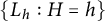 $\{L_h:H=h\}$
in closed connected components, called ovals of H, form continuous families of periodic orbits of the Hamiltonian system associated with H. The question is what is the maximum number of isolated zeros of the Abelian integrals
 $$\begin{align*}I(h)=\int_{L_h}\omega. \end{align*}$$
The Abelian integrals can be viewed in essence as the first-order Melnikov (or Poincaré–Pontryagin–Melnikov) function relevant to a near-Hamiltonian system, obtained by polynomial perturbations of a polynomial Hamiltonian system. The Poincaré–Pontryagin–Melnikov theorem shows that the number of simple isolated zeros of the Abelian integrals provides a lower bound on the maximum number of limit cycles of the near-Hamiltonian system. In this direction, there have appeared lots of published works (see, e.g., [Reference Binyamini, Novikov and Yakovenko5, Reference Chow, Li and Yi7, Reference Christopher and Li8, Reference Gavrilov15, Reference Gavrilov and Iliev16, Reference Grau, Mañosas and Villadelprat18, Reference Han21, Reference Horozov and Iliev28, Reference Li, Li, Llibre and Zhang33, Reference Liu36, Reference Liu and Xiao37, Reference Wang, Wang and Xiao50, Reference Zhang66] and the references therein). But in general, this problem is far to be solved.
As we know, the Abelian integrals strongly depend on the families of ovals
 $\{L_h\}$
. And the families can be limited in different regions. Here, we study a continuous family of ovals, formed by level curves of a Hamiltonian, which are limited in a unique region bounded by a nilpotent center and a homoclinic loop to a nilpotent singularity.
Consider an analytic differential system of the form:
 $$ \begin{align} \begin{cases} \dot{x}=\ \ H_{y}(x,y)+\varepsilon P_0(x,y,\varepsilon,\delta),\\ \dot{y}=-H_{x}(x,y)+\varepsilon Q_0(x,y,\varepsilon,\delta), \end{cases} \end{align} $$
with
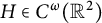 $H\in C^{\omega }(\mathbb R^{2})$
and
 $P_0, Q_0\in C^{\omega }(\mathbb R^{2}\times I\times D)$
, where
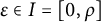 $\varepsilon \in I=[0,\rho ]$
with
 $\rho>0$
small and
 $\delta \in D\subset \mathbb R^{d}$
a compact subset in the real d-dimensional space. The origin is a nilpotent singularity of the unperturbed Hamiltonian system (1)
 $|_{\varepsilon =0}$
, if the Hamiltonian H satisfies
 $H_x(0,0)=H_y(0,0)=0$
and
 $$\begin{align*}\frac{\partial(H_y,-H_x)}{\partial(x,y)}(0,0)\neq0,\qquad \mathrm{det}\frac{\partial(H_y,-H_x)}{\partial(x,y)}(0,0)=0.\end{align*}$$
As it is well known, if a singularity of system (1) is nilpotent, there exists an invertible real linear change of variables under which system (1) is transformed to a new one, whose linear part has the matrix
 $$\begin{align*}\begin{pmatrix}0&2h_{00}\\0&0\end{pmatrix}, \end{align*}$$
with
 $h_{00}$
nonzero. Without loss of generality, we set the nilpotent singularity at the origin. And system (1) has its linear part in the above normal form. Then, the unperturbed Hamiltonian is of the form
 $H(x,y)=h_{00}y^2+\mathrm {h.o.t.}$
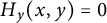
, where h.o.t. represents the higher-order terms. By [Reference Dumortier, Llibre and Artés11, Reference Zhang, Ding, Huang and Dong67], applying the implicit function theorem to
 $H_y(x,y)=0$
in a neighborhood of the origin yields a unique analytic solution
 $y=\phi (x)$
, defined in a neighborhood of
 $x=0$
. Therefore, the Hamiltonian H, without loss of generality, can be written in
 $$ \begin{align} H(x,y)=H_{0}(x)+y^{2}{\widetilde{H}}(x,y), \end{align} $$
where
 $$ \begin{align} H_0(x)=\sum_{j\geq k}h_{j}x^{j},\qquad \widetilde{H}(x,y)=\sum_{j\geq0}H^{\ast}_jy^j,\qquad H^{\ast}_j=\sum_{i\geq0}{h_{ij}x^{i}}, \end{align} $$
with
 $h_k$
(
 $k\in \mathbb N$
and
 $k\ge 3$
) and
 $h_{00}$
nonzero constants provided that the origin is a nilpotent singularity. For more information on nilpotent singularities, see, e.g., [Reference Dumortier, Llibre and Artés11, Reference Han21, Reference Perko40, Reference Zhang, Ding, Huang and Dong67]. Here, we list the ones that we need. We remark that in the next Proposition 1 and Lemmas 1–3, we use
 $h_{00}$
as a nonzero constant, but it was given by Han [Reference Han21] in its original statement taking
 $h_{00}=1/2$
. We must say that this is not essentially different. In the lemmas, the clockwise orientation of the homoclinic loop or periodic orbits near the nilpotent center implies
 $h_{00}>0$
.
Proposition 1 [Reference Han21]
Let the origin be a nilpotent singularity of the unperturbed system (1)
 $|_{\varepsilon =0}$
, and the corresponding Hamiltonian has the form (2) with (3). Then, the origin is a nilpotent center of order m for the unperturbed system (1)
 $|_{\varepsilon =0}$
if
 $k=2m+2$
and
 $h_kh_{00}>0$
. The origin is a nilpotent saddle of order m if
 $k=2m+2$
and
 $h_kh_{00}<0$
. The origin is a cusp of order m if
 $k=2m+1$
and
 $h_kh_{00}\neq 0$
.
Associated with the forms (2) and (3) via Proposition 1, one has
 $k\geq 3$
(i.e.
 $m\geq 1$
). When
 $k=2$
(i.e.,
 $m=0$
), the origin is a hyperbolic saddle if
 $h_kh_{00}<0$
, or else is an elementary center. As mentioned before, we suppose that the unperturbed system (1)
 $|_{\varepsilon =0}$
has the structure on the orbits:
-
(a) A continuous family of periodic orbits
 $\left \{L^1_h\right \}\subset \left \{(x,y):H(x,y)=h\right \}$
, which forms a period annulus, denoted by
$U_1$
.
-
(b) A homoclinic loop
$L_s$
to a nilpotent singularity S, which forms the outer boundary of the annulus
$U_1$
. -
(c) A nilpotent center C, which is the inner boundary of
$U_1$
.



These assumptions together with the expression of H in (2) imply that the Hamiltonian system (1)
 $|_{\varepsilon =0}$
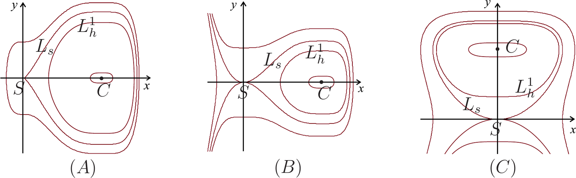
has the phase portrait as shown in Figure 1.
The phase portrait of the Hamiltonian system (1)
 $|_{\varepsilon =0}$
consisting of a nilpotent center C and a homoclinic loop to a nilpotent singularity S enclosing a period annulus. (A) The nilpotent singularity S is a cusp. (B) and (C) The nilpotent singularity S is a nilpotent saddle.

In this article, we study the limit cycle bifurcation for the first two cases in Figure 1. The third one will be handled in a separate article, because of the length of this article and some technical difference. Without loss of generality, we suppose that the nilpotent saddle is
 $S=(0,0)$
, and the nilpotent center is
 $C=(x_c,0)$
with
 $x_c{>}0$
, and that the homoclinic loop
 $L_s$
is oriented in clockwise in the positive sense. For
 $h_s:=H(0,0)=0$
and
 $h_c :=H(x_c,0)$
, one has
 $h_{c}{<}h{}_{s}$
.
Associated with the family of periodic orbits
 $\{L^1_h, h\in (h_c,h_s)\}$
of the unperturbed system (1)
 $|_{\varepsilon =0}$
, the first-order Melnikov function is
 $$ \begin{align} {}M(h,\delta)=\oint_{L{}^1{}_{h}}(Q_0{\text{d}}x-P_0{\text{d}}y)|_{\varepsilon=0},\qquad\qquad h\in(h{}_c,h{}_s). \end{align} $$
It is well known that the number of limit cycles of system (1) could be found partially through the first-order Melnikov function if it is not zero identically. The coefficients of the expansion of the Melnikov function in h play an essential role in determining the number of limit cycles.
The next three results exhibit the expressions of the expansions of the first-order Melnikov function near a homoclinic loop to a nilpotent singularity or near a nilpotent center. The first one is on the expansion near a homoclinic loop to a nilpotent saddle.
Lemma 1 [Reference Han, Yang and Xiao26, Reference Zang, Han and Xiao65]
For the analytic near-Hamiltonian system (1), whose Hamiltonian H has an oriented clockwise homoclinic loop and is of the form (2) with (3),
 $k\geq 4$
even and
 $h_{k}<0$
, the first-order Melnikov function near and inside the loop
 $L_s$
has the asymptotic expression
 $$ \begin{align} M(h,\delta)&=-\frac{1 }{2k}h\ln |h| I^*_{1,\frac{k}{2}-1}(h,\delta)\nonumber\\&\quad +|h|^{\frac{1}{2}}\sum^{k-1}_{r=1\atop r\neq\frac{k}{2}}A_{r-1}I^*_{1,r-1}(h,\delta)|h|^{\frac{r}{k}} +\psi(h,\delta),\qquad 0 < -h \ll 1, \end{align} $$
where
 $\psi (h,\delta ), I^{*}_{1r}(h,\delta ), r=0,1,\ldots ,k-2,$
are analytic functions in
 $(h,\delta )$
for
 $|h|$
small and
 $\delta \in D$
, and
 $A_{r}$
’s are constants for
 $0\leq r\leq k-2$
and
 $r\neq \frac {k}{2}-1$
.
We remark that, for concrete systems, we need to compute the coefficients in the asymptotic expansions in h of the analytic functions
 $\psi (h,\delta )$
and
 $I^{*}_{1r}(h,\delta )$
’s. Of course, these coefficients are in general analytic functions in
 $\delta $
. For more information on
 $I^{*}_{1r}(h,\delta )$
’s and
 $A_r$
’s, see page 7 of [Reference Han, Yang and Xiao26] or page 2731 of [Reference Wei and Zhang52].
The second one is on the expansion of the Melnikov function near a homoclinic loop to a cusp.
Lemma 2 [Reference Han, Zang and Yang27]
For the analytic near-Hamiltonian system (1), whose Hamiltonian H has an oriented clockwise homoclinic loop and is of the form (2) with (3),
 $k\geq 3$
odd and
 $h_k<0$
, the first-order Melnikov function near and inside the loop
 $L_s$
has the expansion
 $$ \begin{align} M(h,\delta)=|h|^{\frac{1}{2}}\sum^{k-1}_{r=1}\varphi_{r}(h,\delta)|h|^{\frac{r}{k}} +\varphi(h,\delta),\qquad 0<-h\ll1, \end{align} $$
where
 $\varphi (h,\delta ), \varphi _{r}(h,\delta ), r=1,2,\ldots ,k-1,$
are analytic functions in
 $(h,\delta )$
for
 $|h|$
small and
 $\delta \in D$
.
As remarked for Lemma 1, when applied to concrete systems, we need to further compute the coefficients of asymptotic expansions in h for
 $\varphi (h,\delta )$
and
 $\varphi _{r}(h,\delta )$
’s. In Lemmas 1 and 2, we have the condition
 $0<-h\ll 1$
. It is due to the fact that the assumption “
 $L_s$
is oriented in clockwise” implies
 $h<0$
.
The third one is on the expansion of the Melnikov function near a nilpotent center.
Lemma 3 [Reference Han, Jiang and Zhu23]
For the analytic differential system (1) with the Hamiltonian H being of the form (2) with (3),
 $k\geq 4$
even and
 $h_k>0$
, the first-order Melnikov function near a nilpotent center at the origin, with oriented clockwise periodic orbits nearby, has the expression
 $$ \begin{align*} M(h,\delta)=h^{\frac{2+k}{2k}}N(h^{\frac{2}{k}},\delta),\qquad\qquad 0<h\ll1, \end{align*} $$
where
 $N(u,\delta )\in C^\omega $
is of the form
 $$ \begin{align} N(h^{\frac{2}{k}},\delta)= \sum\limits_{r\geq0}C^0_{r}(\delta)h^{\frac{2r}{k}}, \end{align} $$
with
 $$ \begin{align} C^0_r(\delta)=\sum\limits_{i+\frac{k}{2}j=r}r_{ij}(\delta)\beta_{ij},\quad \beta_{ij}=\int^1_0u^{2i}(1-u^k)^{\frac{2j+1}{2}}\mathrm{d}u \end{align} $$
and
 $r_{ij}$
’s depending on
 $\delta $
are given in (2.26).
It is evident that the concrete coefficients in the expansion of the first-order Melnikov function play a central role in studying limit cycles bifurcating from periodic orbits near a homoclinic loop or a center. For the first-order Melnikov function (5) in Lemma 1, Han et al. [Reference Han, Yang and Xiao26] in 2012 came up with an algorithm to compute the coefficients of the first two terms in the expression (5) by virtue of the Maple program, and presented the expressions of the coefficients of
 $h^0$
and
 $h^1$
in the asymptotic expansion of
 $\psi (h,\delta )$
in (5) with
 $k=4$
. Yang et al. [Reference Yang, Yu and Han63] in 2019 indicated the form of the
 $(k+1)$
th coefficient in the expansion of the Melnikov function (5) for even
 $k\geq 4$
, and consequently the explicit expressions of the first
 $k+1$
coefficients can be theoretically obtained via the algorithm in [Reference Han, Yang and Xiao26] by using the Maple program. Wei and Zhang [Reference Wei and Zhang52] in 2020 further displayed the definite expressions of the first
 $k+1$
coefficients in the expansion of the Melnikov function (5) for even
 $k\geq 4$
. For the first-order Melnikov function (6) in Lemma 2, the authors in [Reference Atabaigi, Zangeneh and Kazemi3, Reference Han, Zang and Yang27] exhibited the coefficients of the terms with degree less than 2 in the asymptotic expansion of the function (6) for
 $k=3,5$
. Xiong [Reference Xiong56] in 2015 obtained the properties of the coefficients of the first two terms in the expansion of
 $\varphi (h,\delta )$
in the Melnikov function (6) for odd
 $k\geq 7$
, and pointed out that the coefficients of the other terms with degree less than
 $2$
, in the function (6), can be calculated using the deductive process in [Reference Han, Zang and Yang27]. Wei and Zhang [Reference Wei and Zhang52] in 2020 represented
 $\varphi _{r}(h,\delta )$
in (6) as
 $A_{r-1}I^*_{1,r-1}(h,\delta )$
to simplify the calculations (see Lemmas 4 and 8), and depicted the expressions of the first
 $k+1$
coefficients in the asymptotic expansion of the Melnikov function (6) for odd
 $k\geq 3$
.
All the results listed above are on the coefficients of the terms having lower degrees in the expansion of the first-order Melnikov functions. Wei and Zhang [Reference Wei and Zhang52] and Yang et al. [Reference Yang, Yu and Han64] characterized all coefficients in the asymptotic expansion of the Melnikov function (5) or (6) under some conditions, one of which is that the Hamiltonian system (1)
 $|_{\varepsilon =0}$
has an elementary center inside the loop. When the Hamiltonian system (1)
 $|_{\varepsilon =0}$
has a homoclinic loop enclosing a period annulus with its inner boundary a nilpotent center, the results in [Reference Wei and Zhang52, Reference Yang, Yu and Han64] do not hold. One of our main goals in this article is to tackle this problem. That is, when system (1)
 $|_{\varepsilon =0}$
has a homoclinic loop to a nilpotent singularity, which surrounds a nilpotent center, we develop the existed techniques to obtain the expressions of the coefficients of the terms with higher degrees in the expansion of the first-order Melnikov function near the homoclinic loop via the nilpotent center. To achieve this goal, we need to combine the coefficients of the terms in the expansion of the first-order Melnikov function near the nilpotent center.
Han et al. [Reference Han, Jiang and Zhu23] in 2008 provided an algorithm to compute the coefficients in the asymptotic expansion (7) of the first-order Melnikov function near the center and described the expressions of the first four coefficients with
 $k=4$
. However, for even
 $k\geq 6,$
there are no explicit expressions for the coefficients appearing in the function (7).
Our first result is on the first
 ${k}/{2}$
coefficients in the expansion of the first-order Melnikov function near a nilpotent center.
Theorem 1 For the asymptotic expansion of the first-order Melnikov function given in Lemma 3, the first
 ${k}/{2}$
coefficients
 $C_r^0$
,
 $r\in \{0,1, \ldots , {k}/{2}-1\}$
, have the general formula
 $$ \begin{align*} C^0_r=\frac{1}{k}\mathrm{ B}\left(\frac{2r+1}{k},\frac{3}{2}\right)\sum\limits_{l=0}^{2r}\frac{d_{rl}}{l!}\frac{\partial^l}{\partial x^l} \left.\left(\frac{\partial P_0}{\partial x}+\frac{\partial Q_0}{\partial y}\right)\right|_{(C,\delta)}, \end{align*} $$
where
 $\mathrm {B}(\cdot ,\cdot )$
stands for the
 ${Beta}$
function, and
 $d_{rl}$
’s,
 $l=0,1,\ldots ,2r$
, are given in Lemma 4 below.
On the appearance of the Beta function, see Proposition 2 and the remark under the proof of this proposition below. We must say that the expressions on the coefficients in Theorem 1 are the key point in the proofs of our main results in this article.
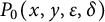
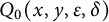
Next, we further investigate the coefficients of the terms with higher degrees in the asymptotic expansions of the first-order Melnikov functions near a homoclinic loop to a nilpotent singularity and near a nilpotent center presented in Lemmas 1–3. For the analytic near-Hamiltonian system (1), to convert the coefficients of the higher degree terms in the first-order Melnikov function into the coefficients of the lower degree terms for new near-Hamiltonian systems, replacing the perturbations
 $P_0(x,y,\varepsilon ,\delta )$
and
 $Q_0(x,y,\varepsilon ,\delta )$
by new ones, saying the analytic perturbations
 $P_i(x,y,\delta )$
and
 $Q_i(x,y,\delta )$
,
 $i\in \mathbb {N}$
, one gets a new near-Hamiltonian system for each
 $i\in \mathbb N,$
 $$ \begin{align} \begin{cases} \dot{x}=\ \ H_{y}(x,y)+\varepsilon P_i(x,y,\delta),\\ \dot{y}=-H_{x}(x,y)+\varepsilon Q_i(x,y,\delta). \end{cases} \end{align} $$
Under these notations, we expand the analytic function
 $I_{1r}^*$
’s,
 $\psi , \varphi $
and
 $\varphi _r$
’s in Lemmas 1 and 2 in Taylor series in h, we get the next asymptotic expressions of the first-order Melnikov function near and inside the homoclinic loop
 $L_s$
either as
 $$ \begin{align} M^i(h,\delta)=&B^i_0+|h|^{\frac{1}{2}}\sum\limits_{j\geq0}\sum^{k_1j+\frac{k_1}{2}-1}_{r=k_1j+1}B^i_r|h|^{\frac{r}{k_1}}+\sum\limits_{j\geq0}B^i_{k_1j+\frac{k_1}{2}}h^{j+1}\ln |h|\nonumber\\ & \qquad\qquad+|h|^{\frac{1}{2}}\sum\limits_{j\geq0}\sum\limits^{(j+1)k_1-1}_{r=k_1j+\frac{k_1}{2}}B^i_{r+1}|h|^{\frac{r}{k_1}},\qquad 0<-h\ll1, \end{align} $$
for
 $L_s$
to a nilpotent saddle S of order
 $[\frac {k_1-1}{2}]$
with even
 $k_1$
, or as
 $$ \begin{align} M^i(h,\delta)=&B^i_0+|h|^{\frac{1}{2}}\sum\limits_{j\geq0}\sum^{k_1j+\frac{k_1-1}{2}}_{r=k_1j+1}B^i_{r}|h|^{\frac{r}{k_1}}+\sum\limits_{j\geq0}B^i_{k_1j+\frac{k_1+1}{2}}h^{j+1} \nonumber\\ &\qquad\qquad +|h|^{\frac{1}{2}}\sum\limits_{j\geq0}\sum\limits^{(j+1)k_1-1}_{r=k_1j+\frac{k_1+1}{2}}B^i_{r+1}|h|^{\frac{r}{k_1}}, \qquad 0<-h\ll1, \end{align} $$
for
 $L_s$
to a nilpotent cusp S of order
 $[\frac {k_1-1}{2}]$
with odd
 $k_1$
. Recall that
 $[\cdot ]$
denotes the integer part function. In (10) and (11), the coefficients
 $B_j^i$
’s are functions of the parameters
 $\delta $
, which need to be computed. The first
 $k_1+1$
coefficients in the last two expressions had been got in [Reference Wei and Zhang52], and they will be presented in Section 3 for our application.
As mentioned before, the nilpotent center C is located on the x-axis, and the near-Hamiltonian system (1) has its unperturbed one having the Hamiltonian of the form (2) with (3). By Lemma 3, it follows that the first-order Melnikov function near the nilpotent center C, of order
 ${k_2}/{2}-1$
with even
 $k_2$
, can have the asymptotic expansion
 $$ \begin{align} M^i(h,\delta)=(h-h_c)^{\frac{2+k_2}{2k_2}}\sum\limits_{r\geq0}C^i_{r}(h-h_c)^{\frac{2r}{k_2}},\qquad 0\leq h-h_c\ll1. \end{align} $$
The coefficients
 $C^i_r$
’s for
 $r=0,1,\ldots ,\frac {k_2}{2}-1$
can be gained from Lemma 3 through a translation. It can be seen from the expressions of the coefficients
 $C^0_r$
’s in Theorem 1 that when the subscript r increases by
 $1$
, the number of terms in the summation in
 $C^0_r$
increases by
 $2$
. To obtain our main results, we come up with the next new symbols
 $$\begin{align*}C^i_{r1}:=\frac{1}{k}\mathrm{ B}\left(\frac{2r+1}{k},\frac{3}{2}\right)\sum\limits_{l=0}^{r}\frac{d_{r,2l}}{(2l)!}\frac{\partial^{2l}}{\partial x^{2l}} \left. \left(\frac{\partial P_i}{\partial x}+\frac{\partial Q_i}{\partial y}\right)\right|_{(C,\delta)}. \end{align*}$$
Set
 $$ \begin{align*} \Delta^i:=&\left\{\delta:B^i_r(\delta)=0, \quad r=1,2,\dots,\left[\frac{k_1}{2}\right],\left[\frac{k_1}{2}\right]+2,\dots,k_1,\right.\\ &\qquad \left.~C^i_0(\delta)=C^i_j(\delta)=C^i_{j1}(\delta)=0, \quad j=1,2,\dots,\frac{k_2}{2}-1\right\},\\ \overline{\Delta}^i:=&\bigcap_{s=0}^{i}\Delta^s. \end{align*} $$
Our second result is to characterize the coefficients of the terms with higher degrees in the asymptotic expansion of the first-order Melnikov function (4) near a homoclinic loop to a nilpotent singularity for the near-Hamiltonian system (1). It combines the asymptotic expansion of the first-order Melnikov function at the nilpotent center.
Theorem 2 For the analytic near-Hamiltonian system (1), whose unperturbed Hamiltonian is of the form (2) with (3), and has a nilpotent center of order
 $\frac {k_2}{2}-1$
and an oriented clockwise homoclinic loop to a nilpotent singularity of order
 $\left [\frac {k_1-1}{2}\right ]$
, assume that the following conditions hold:
-
(i) The first-order Melnikov function is of the form (10) or (11) with
$i=0$
near the loop, or of the form (12) with
$i=0$
near the center. -
(ii) There exist analytic functions
$P_i(x,y,\delta )$
and
$Q_i(x,y,\delta )$
for
$i=1,2,\ldots ,l,$
such that for
$\delta \in \overline {\Delta }^{i-1}$
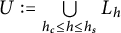
, the following equalities inductively hold: (13)over the period annulus
$$ \begin{align} \frac{\partial H(x,y)}{\partial x}P_i(x,y,\delta)+\frac{\partial H(x,y)}{\partial y}Q_i(x,y,\delta) = \left(\frac{\partial P_{i-1}}{\partial x}+\frac{\partial Q_{i-1}}{\partial y}\right)(x,y,\delta), \end{align} $$
$U:=\bigcup \limits _{h_c\leq h\leq h_s}L_h$
, where
$P_0(x,y,\delta )$
and
$Q_0(x,y,\delta )$
are just
$P_0(x,y,0,\delta )$
and
$Q_0(x,y,0,\delta )$
in system (1), respectively.







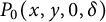
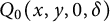
Then, the coefficients in the first-order Melnikov function, given in (10)–(12), of system (1) satisfy the following formulas for
 $\delta \in \overline {\Delta }^{i-1}$
, in which
 $B^i_j$
’s are given in (2.33) below.
-
(a) For
$r=1,2,\dots ,[\frac {k_1-1}{2}]$
,
$$ \begin{align*} B^0_{k_1i+r}=\frac{(-1)^i(2k_1)^i}{\prod\limits^i_{j=1}((2j+1)k_1+2r)}B^i_r. \end{align*} $$
-
(b) For
$r=[\frac {k_1+1}{2}]$
,
$$ \begin{align*} B^0_{k_1i+r}=\frac{1}{(i+1)!}B^i_r. \end{align*} $$
-
(c) For
$r=\frac {k_1}{2}+1 ($
in the case that
$k_1$
is odd, this statement is void
$)$
$$ \begin{align*} B^0_{k_1i+r}=\frac{(-1)^i}{(i+1)!}B^i_r+\frac{(-1)^i}{(i+1)!}\left(\sum\limits^{i+1}_{n=2}\frac{1}{n}\right)B^i_{r-1}. \end{align*} $$
-
(d) For
$r=[\frac {k_1}{2}]+2,\ldots ,k_1$
,
$$ \begin{align*} B^0_{k_1i+r}=\frac{(-1)^i(2k_1)^i}{\prod\limits^i_{j=1}((2j+1)k_1+2r-2)}B^i_r. \end{align*} $$
-
(e) For
$j=0,1,\dots , \frac {k_2}{2}-1$
,
$$ \begin{align*} C^0_{\frac{k_2}{2}i+j}=\frac{(2k_2)^i}{\prod\limits^i_{s=1}((2s+1)k_2+4j+2)}C^i_j. \end{align*} $$







We remark that the properties in the above theorem have been partly acquired by Tian and Han [Reference Tian and Han48] and Wei et al. [Reference Wei, Zhang and Zhang51] for
 $k_1=k_2=2$
, in which the center is an elementary one and the singularity that the homoclinic loop approaches is a hyperbolic saddle (see Page 2). And the properties have been presented by Wei and Zhang [Reference Wei and Zhang52] for
 $k_2=2, k_1\geq 3$
, in which the center in Theorem 2 is an elementary one and the loop is homoclinic to a nilpotent singularity of order
 $[\frac {k_1-1}{2}]$
.
The result in Theorem 2 characterizes parts of the coefficients in the asymptotic expansion of the first-order Melnikov function (4) near a homoclinic loop under some condition by utilizing the properties of the nilpotent center and also parts of the coefficients in the expansion near the nilpotent center. In other words, we could say that the result of the theorem indicates the properties on the coefficients in the expansion near a nilpotent center via a homocinic loop. Following this idea, we can think only about the properties of the coefficients in the Melnikov function near a nilpotent center without regard to a homoclinic loop.
The next result presents the properties near a nilpotent center. Its proof can be obtained in a similar way as that in the proof of Theorem 2 given in Section 3. The details are omitted.
Set
 $$ \begin{align*} \overline{\Lambda}^i:=\bigcap_{s=0}^{i}\Lambda^s \ \ \ \text{ with }\ \ \ \Lambda^i:=\left\{\delta: \ C^i_0(\delta)=C^i_j(\delta)=C^i_{j1}(\delta)=0, j=1,2,\dots,\frac{k_2}{2}-1\right\}. \end{align*} $$
Theorem 3 For the analytic near-Hamiltonian system (1) with its unperturbed one being of the form (2) with (3) and having a nilpotent center of order
 $\frac {k_2}{2}-1$
with oriented clockwise periodic orbits nearby, assume that the following conditions hold:
-
(i) The first-order Melnikov function has the expansion of the form (7) near the center.
-
(ii) There exist analytic functions
$P_i(x,y,\delta )$
and
$Q_i(x,y,\delta )$
for
$i=1,2,\ldots ,l,$
such that for
$\delta \in \overline {\Lambda }^{i-1}$
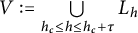
, the equations (13) hold over the period annulus
$V:=\bigcup \limits _{h_c\leq h\leq h_c+\tau }L_h$
with
$0<\tau \ll 1$
.





Then, the coefficients
 $C^0_j,j\geq {k_2}/{2}$
, in the expansion (12) of the first-order Melnikov function satisfy the following relations:
 $$ \begin{align*} \left.C^0_{\frac{k_2}{2}i+r}\right|_{\delta\in\overline{\Lambda}^{i-1}}=\frac{(2k_2)^i}{\prod\limits^i_{s=1}((2s+1)k_2+4r+2)}C^i_r, \end{align*} $$
for
 $r=0,1,\dots ,\frac {k_2}{2}-1$
, where
 $C^i_r$
’s are the coefficients in the expansion (12).
We remark that the conclusion in Theorem 3 is not different from that in (e) of Theorem 2. The differences are in the following aspects: Theorem 3 focuses on the coefficients in the asymptotic expansion of the first-order Melnikov function near a nilpotent center, so the restriction
 $\delta \in \overline {\Lambda }^{i-1}$
there is only for the coefficients of the terms with lower degrees in the expansion just near the nilpotent center. Whereas Theorem 2 handles the coefficients in the expansion of the Melnikov function near the homoclinic loop or near the nilpotent center, in which the restriction
 $\delta \in \overline {\Delta }^{i-1}$
is on both coefficients of the terms with lower degrees in the expansions near the loop and near the center. It leads to interdependent relationships among the coefficients in the expansions near the loop and near the center.
The last two theorems display the relative expressions of parts of the coefficients in the asymptotic expansion of the first-order Melnikov function under the prescribed conditions, which is crucial in finding more limit cycles of the system. The next result explains the realizability of the conditions in Theorem 2, especially the conditions (13) for
 $i\geq 1$
, for a certain kind of analytic near-Hamiltonian systems. We remark that the condition
 $\delta \in \overline {\Delta }^{i-1}$
under which equation (13) holds is different from that in Tian and Han [Reference Tian and Han48], where the realization is explained under the condition
 $H(x,y)=\int _{0}^{x}q(x)\mathrm {d}x+\int _{0}^{y}p(y)\mathrm {d}y$
. Here, we do not have this limitation for the Hamiltonian.
Theorem 4 Assume that the Hamiltonian
 $H(x,y)$
satisfies condition
 $(i)$
of Theorem 2, and
 $\frac {\partial H}{\partial y}(x,y)/y$
does not vanish in U defined in Theorem 2. For any analytic 1-form
 $\omega =P\mathrm {d}y-Q\mathrm {d}x$
, if its exterior derivative
 $\mathrm {d}\omega =f(x,y)\mathrm {d}x\wedge \mathrm {d}y$
satisfies
 $f(x,0)=x^{k_1-1}(x-x_c)^{k_2-1}\mu (x)$
with
 $\mu (x)$
analytic in U, then there exists an analytic 1-form
 $\eta =A\mathrm {d}y-B\mathrm {d}x$
such that
 $$\begin{align*}\mathrm{d}\omega=\mathrm{d}H\wedge\eta.\end{align*}$$
This result is an extension of Theorem 6 in [Reference Wei and Zhang52] from an elementary center to a nilpotent center. The proof is also similar to that in [Reference Wei and Zhang52], and will be omitted. Analogously, the conditions in Theorem 3 are also realizable for some near-Hamiltonian systems.
Finally, we apply our main results in Theorems 2 and 3 and the theories on limit cycle bifurcation to find more limit cycles via the number of simple isolated zeros of the Abelian integral (the first-order Melnikov function), related to the two classes of near–Hamiltonian systems. Givental [Reference Givental17] found some nonoscillation-type properties of Abelian integrals in the hyperelliptic Hamiltonian
 $H(x,y)=y^2+U_{n+1}(x)$
with a real polynomial
 $U_{n+1}(x)$
in x of degree
 $n+1$
. Here, our perturbed Hamiltonian systems are also defined by hyperelliptic Hamiltonians.
Hereafter, we use the notion
 $\mathrm {mod}(a,b)$
to denote the remainder of a divided by b.
Consider a generalized polynomial Liénard differential system of the form
 $$ \begin{align} \dot x=y,\qquad \dot y=-g_n(x)+\varepsilon yf_m(x), \end{align} $$
where
 $\varepsilon>0$
is sufficiently small, and
 $g_n$
and
 $f_m$
are real polynomials of degrees n and m, respectively. Denote by
 $Z(n,m)$
the maximum number of isolated zeros of the Abelian integral associated with the generalized Liénard system (14). On determination of
 $Z(n,m)$
, there are rich results for
 $n=1,2,3,4$
(see, e.g., [Reference Bogdanov6, Reference Dadfar, Geer and Andersen9, Reference Dumortier and Li10, Reference Dumortier, Roussarie and Sotomayor12, Reference Gavrilov and Iliev16, Reference Han22, Reference Itikawa, Oliveira and Torregrosa30, Reference Llibre, Mereu and Teixeira38, Reference Petrov41, Reference Sun and Yu46, Reference Wang and Xiao49, Reference Wang, Wang and Xiao50, Reference Wei and Zhang53, Reference Wei, Zhang and Zhu54, Reference Xiong57] and the references therein).
For
 $n=5$
, Xu and Li [Reference Xu and Li59] in 2012 got
 $Z(5,m)\geq m+1$
for
 $m=2,4$
and
 $Z(5,m)\geq 10$
for
 $m=6,8$
, where the unperturbed Hamiltonian system includes two elementary centers and a double homoclinic loop surrounded by a heteroclinic to two hyperbolic saddles. Xu and Li [Reference Xu and Li60] in 2013 gained
 $Z(5,m)\geq m+\mathrm {mod}(m/2,2)$
for
 $m=4,6,10,$
when the period annulus is bounded by a compound loop consisting of a heteroclinic loop and two homoclinic loops. Han and Romanovski [Reference Han and Romanovski24] in 2013 achieved
 $Z(5,m)\geq 2[\frac {m-1}{3}]+[\frac {m-1}{2}]$
using a different approach for
 $m\geq 5$
. Sun et al. [Reference Sun, Xi, Zangeneh and Kazemi45, Reference Sun and Yu47] presented
 $Z(5,4)\geq 3$
in the case that the period annulus is limited by an elementary center and a heteroclinic loop to a hyperbolic saddle and a nilpotent saddle, respectively. Xiong [Reference Xiong55] in 2014 showed
 $Z(5,m)\geq 2m+1$
for
 $m=2,3,4,$
and
 $Z(5,m)\geq m+5$
for
 $5\leq m\leq 8$
in the case that the period annulus is limited by two elementary centers and a compound loop consisting of a cuspidal loop and a heteroclinic loop with a cusp and a hyperbolic saddle. In the same year, Xiong and Han [Reference Xiong and Han58] further got
 $Z(5,m)\geq 2[\frac {m-1}{3}]+[\frac {m}{2}]+2$
for
 $m\geq 5$
. Li and Yang [Reference Li and Yang35] in 2019 provided also the lower bounds of
 $Z(5,m)$
in the case that the unperturbed Hamiltonian system is the same as that of [Reference Xiong55] for
 $10\leq m\leq 20$
. Yang et al. [Reference Yang, Yu and Han64] in 2021 achieved that for
 $22\leq m\leq 46$
even,
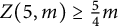 $Z(5,m)\geq \frac {5}{4}m$
if
 $4|m$
and
 $Z(5,m)\geq \frac {5}{4}m-\frac {1}{2}+[\frac {\mathrm {mod}(m/2,4)}{2}]$
if
 $4\nmid m$
, under the conditions that the corresponding Liénard system (14) is centrally symmetric and has two centers and a double homoclinic loop with a nilpotent saddle, and that for
 $22\leq m\leq 46$
odd,
 $Z(5,m)\geq Z(5,m-1)$
. Yang and Han [Reference Yang and Han62] in 2024 gave further in the case of an elementary center and a cuspidal loop passing a cusp of order 2 that, for
 $15\leq m\leq 25,$
a lower bound is
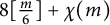 $8[\frac {m}{6}]+\chi (m)$
with
 $\chi (m)=2\ \mathrm {mod}(m,6)+1$
if
 $\mathrm {mod}(m,6)\leq 3$
and
 $\chi (m)=8$
if
 $\mathrm {mod}(m,6)\geq 4$
. For
 $n\geq 6$
, there are also some works on the lower bound of the number of isolated zeros (see, e.g., [Reference Bakhshalizadeh, Asheghi, Zangeneh and Ezatpanah Gashti4, Reference Han and Romanovski24, Reference Han and Yang25, Reference Sun44, Reference Xiong56, Reference Xiong and Han58] and the references therein).
Next, we apply our results on the expressions of the first-order Melnikov functions to study the Liénard system (14) with
 $g_5=x^2(x-1)^3$
for obtaining a better low bound on
 $Z(5,m)$
.
Theorem 5 There exists a generalized Liénard system of the form (14) with
 $n=5$
and
 $g_5=x^2(x-1)^3$
, which has at least
 $7\cdot [\frac {m-1}{6}]+2r-\left [\frac {r}{4}\right ]\cdot (2\ \mathrm {mod}(r,3)-1)-1$
limit cycles with
 $r=\mathrm {mod}(m-1,6)$
and
 $4\leq m\leq 300$
.
Recall that
 $\mathrm {mod}(a,b)$
denotes the remainder of a divided by b. This theorem provides a larger lower bound on
 $Z(5,m)$
than those in [Reference Han and Romanovski24] with
 $Z(5,m)\geq 2[\frac {m-1}{3}]+[\frac {m-1}{2}]$
.
For the Hamiltonian system having a nilpotent center, Llibre and Zhang [Reference Llibre and Zhang39] in 2001 considered the degree m polynomial perturbation of the Hamiltonian center with the Hamiltonian
 $H(x,y)=\frac {1}{2n}x^{2n}+\frac {1}{2l}y^{2l}$
, and gained the number s if
 $n=l$
;
 $\frac {s(s+3)}{2}$
if
 $s<k$
and
 $n\neq l$
; and
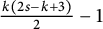 $\frac {k(2s-k+3)}{2}-1$
if
 $s\geq k$
and
 $n\neq l$
, of isolated zeros of the Abelian integrals, where
 $s=[\frac {m-1}{2}]$
and
 $k=\max \{n/\gcd (n,l),l/\gcd (n,l)\}$
with the greatest common divisor
 $\gcd (n,l)$
. Jiang et al. [Reference Jiang, Zhang and Han32] in 2009 studied the same problem in a centrally symmetric case with
 $n=2,l=1, m=5$
, and got ten isolated zeros by blowing up a nilpotent center of order 1 to a double homoclinic loop. Su et al. [Reference Su, Yang and Han43] in 2012 showed that a generalized Liénard system of degree m can have 1, 3, 5 limit cycles near a nilpotent center of order 1 for
 $m=3,4,5$
. In the same year, Yang and Han [Reference Yang and Han61] figured out that a generalized Liénard system of degree m with the Hamiltonian
 $H(x,y)=\frac {1}{2}y^{2}+\frac {1}{5}x^5-\frac {3}{4}x^{4}+x^3-\frac {1}{2}x^2$
can have
 $m-1-[\frac {m}{5}]$
limit cycles for
 $2\leq m\leq 13$
, which include
 $m-2-[\frac {m}{5}]$
limit cycles near a nilpotent center of order 1. Gasull et al. [Reference Gasull, Yu and Zhang14] in 2015 focused on an
 $\frac {n-1}{2}$
order nilpotent center with the perturbations, linear term plus homogeneous polynomials of odd degree n, whose Abelian integrals can have
 $\frac {n+1}{2}$
isolated zeros around the center with their proof using the generalized Lyapunov polar coordinate change of variables. As far as we know, the limit cycle bifurcation near a nilpotent center was rarely studied.
As a second application, we consider a near-Hamiltonian system (1) with the unperturbed Hamiltonian
 $$ \begin{align} H(x,y)=\frac{1}{2}y^{2}+\frac{1}{4}x^{4}-\frac{1}{5}x^5-\frac{1}{6}x^6, \end{align} $$
and the perturbed polynomials
 $P_0(x,y)$
and
 $Q_0(x,y)$
being of degree m. The unperturbed system has exactly three singularities: a nilpotent center at the origin together with two hyperbolic saddles on its two sides.
Theorem 6 There exists a near-Hamiltonian system (1) with the Hamiltonian (15), which has at least
 $2\cdot [\frac {m+1}{2}]+2\cdot \left [\frac {2\cdot [\frac {m}{2}]-1}{3}\right ]+\mathrm {mod}(2\cdot [\frac {m}{2}]-1,3)-3$
small-amplitude limit cycles near the nilpotent center for
 $3\leq m\leq 22$
.
We remark that there is no published paper which studied this near-Hamiltonian system. The related work is the book [Reference Dumortier, Roussarie, Sotomayor and Żoładek13], in which a generic
 $3$
-parameter unfolding was investigated for planar vector fields with a nilpotent singularity.
The article is organized as follows. In Section 2, we study the first-order Melnikov function near a nilpotent center and a homoclinic loop to a nilpotent singularity, and obtain the exact expressions and the properties of the coefficients in the corresponding asymptotic expansions. The proofs of Theorems 1–3 are also presented in this section. Section 3 studies the relation between the limit cycle bifurcation and the independence of the coefficients obtained in Theorems 1–3. The proofs of Theorems 5 and 6 are given in Section 4.
2 The first-order Melnikov functions near a center and a homoclinic loop
Han et al. [Reference Han, Jiang and Zhu23, Reference Jiang and Han31, Reference Yang and Han61] presented the asymptotic expansions of the first-order Melnikov functions near a nilpotent center, and established an algorithm to compute the coefficients of the Melnikov functions by the Maple program. In this section, we further study the coefficients and optimize their algorithm to simplify the calculations.
Yang and Han [Reference Yang and Han61] in 2012 provided an algorithm to compute the coefficients in the expansion of the first-order Melnikov function near a nilpotent center of order
 $\frac {k}{2}-1$
with the help of the Maple program. There, they need to require a fixed integer k in the process of the Maple program, and it is hard to figure out the explicit expressions of the coefficients with higher degrees due to computer performance limitations. In the present article, for any
 $k\geq 4,$
even the expressions and properties of the first coefficients in the first-order Melnikov function near a nilpotent center are provided and they will play key roles in understanding the coefficients of the terms with higher degrees in the Melnikov function established near a nilpotent center or near a homoclinic loop to a nilpotent singularity. This will provide a nice tool to handle the limit cycles bifurcating from the periodic orbits near the nilpotent center or near the homoclinic loop.
For simplicity to notations, we take
 $x_c=0$
in the first section below, and suppose that the Hamiltonian of the unperturbed system (1)
 $|_{\varepsilon =0}$
is of the form (2) with (3) and
 $h_{00}>0$
. To study the asymptotic expression of the first-order Melnikov functions, without loss of generality, we set the perturbation functions being of the form
 $$ \begin{align} P_0(x,y,0,\delta)=\sum_{i+j\geq0}a_{ij}x^{i}y^{j},\quad Q_0(x,y,0,\delta)=\sum_{i+j\geq0}b_{ij}x^{i}y^{j}, \end{align} $$
where
 $a_{ij}$
and
 $b_{ij}$
are analytic functions in the parameters
 $\delta \in D\subset \mathbb R^d$
.
2.1 The coefficients of the terms with lower degrees
By the classical results [Reference Guckenheimer and Holmes19, Reference Roussarie42] on Melnikov functions for computing limit cycles bifurcating from period annulus, we get from Green’s formula together with some manipulations that the first-order Melnikov function (4) can be rewritten as
 $$ \begin{align} M(h,\delta)=\displaystyle\oint_{H(x,y)=h}\overline{q}(x,y,\delta)\mathrm{d}x, \end{align} $$
where
 $$ \begin{align*} \begin{aligned} \overline{q}(x,y,\delta)&=\displaystyle\int_{0}^{y}\left(\frac{\partial P_0}{\partial x}(x,v,0,\delta)+\frac{\partial Q_0}{\partial y}(x,v,0,\delta)\right)\mathrm{d}v\\ &=Q_0(x,y,0,\delta)-Q_0(x,0,0,\delta)+\displaystyle\int_{0}^{y}\frac{\partial P_0}{\partial x}(x,v,0,\delta)\mathrm{d}v\\ &=\sum\limits_{j\geq1}q_j(x)y^j \end{aligned} \end{align*} $$
with
 $$ \begin{align} q_j(x)=\sum\limits_{i\geq0}\overline{b}_{ij}x^i, \end{align} $$
whose coefficients satisfy
 $$ \begin{align} \overline{b}_{ij}=b_{ij}+\frac{i+1}{j}a_{i+1,j-1}. \end{align} $$
Following [Reference Han, Jiang and Zhu23], we know that the Hamiltonian (2) contains the component
 $\widetilde {H}(x,y)=h_{00}+O(|x,y|)$
. Then,
 $H(x,y)=h$
is equivalent to
 $\omega =|y|(\widetilde {H}(x,y))^{\frac {1}{2}}$
, where
 $\omega =\sqrt {h-H_{0}(x)}$
. Applying the implicit function theorem to it, one gets two locally analytic solutions of
 $H(x,y)=h$
, saying
 $y_{1}(x,\omega )$
and
 $y_{2}(x,\omega )$
, which satisfy
 $y_{1}(x,\omega )=(h_{00})^{-\frac {1}{2}}\omega (1+O(|x,\omega |))=y_{2}(x,-\omega )$
near
 $(x,\omega )=(0,0)$
, and
 $y_1(x,\omega )$
can be expanded in
 $\omega $
as follows:
 $$ \begin{align} y_{1}(x,\omega)=\sum_{i\geq1}a_i(x)\omega^i, \end{align} $$
where
 $$ \begin{align*} a_{1}(x)&= \frac{1}{\sqrt{H^*_1}},\\ a_{i+1}(x)&=-\frac{1}{2\sqrt{H^*_1}}\left(H^*_1\sum\limits_{\substack{t_1+t_2=i+2,\\t_1,t_2\geq2}}a_{t_1}a_{t_2}+\sum\limits^i_{j=1}H^*_{j+1}b^{j+2}_{i+2}\right),\quad \text{for}\quad i\geq 1, \end{align*} $$
with
 $b^j_i=\sum \limits _{t_1+t_2+\cdots +t_j=i}a_{t_1}a_{t_2}\dots a_{t_j}$
, and
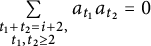 $\sum \limits _{\substack {t_1+t_2=i+2,\\t_1,t_2\geq 2}}a_{t_1}a_{t_2}=0$
if
 $i=1$
.
Under these notations, the integral
 $M(h,\delta )$
in (2.17) can be written in
 $$ \begin{align*} \nonumber M(h,\delta)&=\displaystyle\int^{a(h)}_{b(h)}\left(\overline{q}(x,y_{1}(x,\omega),\delta)-\overline{q}(x,y_{2}(x,\omega),\delta)\right)\mathrm{d}x\\\nonumber &=\displaystyle\int^{a(h)}_{b(h)}\sum_{j\geq1}q_j(x)(y_1^j-y_2^j)\mathrm{d}x, \end{align*} $$
where
 $a(h)$
and
 $b(h)$
are two solutions of the equation
 $H_0(x)=h$
in a neighborhood of
 $x=0$
. The symmetry of
 $y_1$
and
 $y_2$
with respect to the y-axis further simplifies the Melnikov function to
 $$ \begin{align} M(h,\delta)=\displaystyle\int^{a(h)}_{b(h)}\sum_{j\geq0}\overline{q}_j(x)(h-H_{0}(x))^{\frac{2j+1}{2}}\mathrm{d}x, \end{align} $$
where
 $$ \begin{align} \overline{q}_j(x)&=2\sum\limits^{2j}_{i=0}q_{i+1}b^{i+1}_{2j+1}. \end{align} $$
We note that the details about the derivations of (2.20) and (2.21), together with the expressions of
 $ a_1,a_2,a_3$
in (2.20) and
 $\overline {q}_0,\overline {q}_1$
in (2.22), can be found on page 191 or on page 193 of book [Reference Han21].
Introducing a new variable
 $$ \begin{align} u=\mathrm{sgn}(x)\cdot|H_0(x)|^{\frac{1}{k}}:=\Phi(x), \end{align} $$
the Melnikov function can be expressed as
 $$ \begin{align} M(h,\delta)&=\sum_{j\geq0}\displaystyle\int^{h^{\frac{1}{k}}}_{-h^{\frac{1}{k}}}\widetilde{q}_j(u)(h-u^k)^{\frac{2j+1}{2}}\mathrm{d}u\nonumber\\ &=\sum_{j\geq0}\displaystyle\int^{h^{\frac{1}{k}}}_{0}(\widetilde{q}_j(u)+\widetilde{q}_j(-u))(h-u^k)^{\frac{2j+1}{2}}\mathrm{d}u, \end{align} $$
where
 $$ \begin{align} \widetilde{q}_j(u)=\frac{\overline{q}_j(x)}{\Phi'(x)}\Big{|}_{x=\Phi^{-1}(u)} \end{align} $$
can be expanded as a power series in u in a neighborhood of
 $u=0$
, and then
 $$ \begin{align} \widetilde{q}_j(u)+\widetilde{q}_j(-u)=\sum\limits_{i\geq0} r_{ij}u^{2i}, \end{align} $$
with the constants
 $r_{ij}$
’s,
 $i,j\geq 0$
, depending on the coefficients of the perturbations
 $P_0$
and
 $Q_0$
of the analytic near-Hamiltonian system (1). As in [Reference Yang and Han61], substituting (2.26) into (2.24) yields the asymptotic expression in h as in Lemma 3, of the first-order Melnikov function (4) near the nilpotent center.
The next result characterizes the coefficients appearing in Lemma 3.
Proposition 2 The constants
 $\beta _{ij}$
’s given in Lemma 3 have the next expressions
 $$\begin{align*}\beta_{ij}=\frac{1}{k}\mathrm{B}\left(\frac{2i+1}{k},j+\frac{3}{2}\right). \end{align*}$$
Proof The expression
 $\beta _{ij}$
in (8) can be deformed as
 $$ \begin{align*} \beta_{ij}=\int\limits^1_0(u^k)^{\frac{2i}{k}}(1-u^k)^{\frac{2j+1}{2}}\mathrm{d}u. \end{align*} $$
Then, one has
 $$ \begin{align*} \beta_{ij}=\frac{1}{k}\int\limits^1_0t^{\frac{2i+1}{k}-1}(1-t)^{j+\frac{1}{2}}\mathrm{d}t. \end{align*} $$
The proof completes via the definition of the Beta function.
We remark that
 $\beta _{00},\beta _{10},\beta _{20},\beta _{30},\beta _{01},\beta _{11}$
can be obtained from page 198 of [Reference Han21] when
 $k=4$
. Although the expressions are different from those of Proposition 2, they coincide by some calculations. From Lemma 3, one needs to calculate the coefficients
 $C^0_r$
of the first-order Melnikov function, which is the key element in the expressions of
 $r_{ij}$
’s.
Lemma 4 For formula (8) given in Lemma 3, there exist constants
 $d_{il}$
’s,
 $l=0,1,\ldots ,2i$
, depending on the coefficients of the unperturbed Hamiltonian one of system (1), such that for all nonnegative integers i’s,
 $$ \begin{align*} r_{i0}=\sum\limits_{l=0}^{2i}d_{il}\left((l+1)a_{l+1,0}+b_{l1}\right) =\sum\limits_{l=0}^{2i}\frac{d_{il}}{l!}\frac{\partial^l}{\partial x^l} \left.\left(\frac{\partial P_0}{\partial x}+\frac{\partial Q_0}{\partial y}\right)\right|_{(C,\delta)}. \end{align*} $$
In particular,
 $d_{i,2i}=4|h_k|^{-\frac {2i+1}{k}}(h_{00})^{-\frac {1}{2}}$
,
 $d_{i,2i-1}=-\frac {2}{k}((4i+2)h_{k+1}+kh_kh_{10})|h_k|^{-\frac {2i+3}{k}}(h_{00})^{-\frac {1}{2}}$
.
Proof In order to get the expression of
 $r_{i0}$
, we have to know the expansions of the level curves defining the ovals. According to the expression of
 $H_0(x)$
in (3) and the definition of
 $\Phi (x)$
in (2.23), one has
 $$ \begin{align} u=\Phi(x)=|h_k|^{\frac{1}{k}}\sum\limits_{i\geq1}\mu_ix^i, \end{align} $$
whose coefficients
 $\mu _i$
’s,
 $i\geq 2$
depend on
 $h_{j+k}, j=1,\ldots ,i-1$
, and have the expressions
 $$ \begin{align} \mu_i= \begin{cases} 1,&\quad i=1,\\ \sum\limits_{m=1}^{i-1}\frac{(-1)^{m}}{m!(kh_k)^m}\prod\limits^{m-1}_{j=0}(jk-1)\sum\limits_{j_1+\cdots+j_m=i-1}h_{j_1+k}\times\cdots\times h_{j_m+k},&\quad i\geq2. \end{cases} \end{align} $$
Then, it follows from (2.27) that
 $$ \begin{align} \frac{1}{\Phi'(x)} =|h_{k}|^{-\frac{1}{k}}\left(1+\sum\limits_{i\geq1}(i+1)\mu_{i+1}x^i\right)^{-1} =|h_{k}|^{-\frac{1}{k}}\sum\limits_{i\geq0}n_ix^i, \end{align} $$
where
 $n_i, i\geq 1$
, are functions in
 $\mu _2,\ldots ,\mu _{i+1}$
, and have the expressions
 $$ \begin{align*} n_i= \begin{cases} 1,& i=0,\\ \sum\limits_{m=1}^{i}(-1)^m\sum\limits_{j_1+\cdots+j_m=i}(j_1+1)\times\cdots\times(j_m+1)\times\mu_{j_1+1}\times\cdots\times \mu_{j_m+1},& i\geq1, \end{cases} \end{align*} $$
with the positive integers
 $j_l$
’s.
Let
 $x=\Phi ^{-1}(u)$
in (2.25) have the power series in a neighborhood of
 $u=0$
 $$ \begin{align} x=\Phi^{-1}(u)=:\sum\limits_{i\geq1}\overline{\mu}_iu^i. \end{align} $$
By the expression
 $u=\Phi (x)$
in (2.27), equating the next equality
 $$ \begin{align*} u =\Phi(\Phi^{-1}(u)) =|h_k|^{\frac{1}{k}}\sum\limits_{i\geq1}u^i\sum\limits_{m=1}^i\mu_m\sum\limits_{j_1+\cdots+j_m=i}\overline{\mu}_{j_1}\times\cdots\times\overline{\mu}_{j_m} \end{align*} $$
yields
 $$ \begin{align} \overline{\mu}_i= \begin{cases} |h_k|^{-\frac{1}{k}}\mu_1^{-1}=|h_k|^{-\frac{1}{k}},& i=1,\\ -\sum\limits_{m=2}^{i}\mu_m\sum\limits_{j_1+\cdots+j_m=i}\overline{\mu}_{j_1}\times\cdots\times \overline{\mu}_{j_m},& i\geq2, \end{cases} \end{align} $$
with
 $\mu _m$
’s given in (2.28). Now
 $a_1(x)$
, as the first coefficient of
 $y_1(x,\omega )$
in (2.20), via the expression of
 $H^*_0$
in (3), has the asymptotic expansion
 $$ \begin{align} a_{1}(x) &=(h_{00})^{-\frac{1}{2}}\left(1+\sum\limits_{i\geq1}\frac{-\frac{1}{2}(-\frac{1}{2}-1)\dots(-\frac{1}{2}-i+1)}{i!(h_{00})^i}\left(\sum\limits_{j\geq1}h_{j0}x^j\right)^i\right)\nonumber\\ &=(h_{00})^{-\frac{1}{2}}\sum\limits_{i\geq0}x^im_i, \end{align} $$
where
 $m_i$
’s have the expressions
 $$ \begin{align*} m_i= \begin{cases} 1,& i=0,\\ \sum\limits_{l=1}^{i}\frac{-\frac{1}{2}(-\frac{1}{2}-1)\dots(-\frac{1}{2}-l+1)}{l!}\sum\limits_{j_1+\cdots+j_l=i}h_{j_1,0}\times\cdots\times h_{j_l,0},& i\geq1. \end{cases} \end{align*} $$
Substituting (2.18), (2.22), (2.29), and (2.32) into (2.25), we get
 $$ \begin{align*} \widetilde{q}_0(\Phi(x)) &=2|h_k|^{-\frac{1}{k}}(h_{00})^{-\frac{1}{2}}\left(\sum\limits_{i\geq0}\overline{b}_{i1}x^i\right) \left(\sum\limits_{i\geq0}n_{i}x^i\right)\left(\sum\limits_{i\geq0}m_{i}x^i\right)\nonumber\\ &=2|h_k|^{-\frac{1}{k}}(h_{00})^{-\frac{1}{2}}\sum\limits_{i\geq0}x^it_i, \end{align*} $$
where
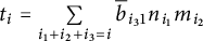 $t_i=\sum \limits _{i_1+i_2+i_3=i}\overline {b}_{i_3 1}n_{i_1}m_{i_2}$
,
 $i_1,i_2,i_3\geq 0$
with
 $\overline b_{j1}$
,
 $n_{j}$
, and
 $m_{j}$
appearing, respectively, in (2.19), (2.29), and (2.21). In particular,
 $t_0=\overline {b}_{01}$
. Substituting (2.30) into the above expression gives
 $$ \begin{align*} \widetilde{q}_0(u) =2|h_k|^{-\frac{1}{k}}(h_{00})^{-\frac{1}{2}}\left(t_0+\sum\limits_{i\geq1}u^i\sum\limits_{m\geq1}^it_m\sum\limits_{j_1+\cdots+j_m=i} \overline{\mu}_{j_1}\times\cdots\times\overline{\mu}_{j_m}\right).\nonumber \end{align*} $$
Combining this expression with (2.26) yields
 $$ \begin{align*} r_{00}&=4|h_k|^{-\frac{1}{k}}(h_{00})^{-\frac{1}{2}}t_0=d_{00}\overline{b}_{01},\nonumber\\ r_{i0}&=4|h_k|^{-\frac{1}{k}}(h_{00})^{-\frac{1}{2}}\sum\limits_{m\geq1}^{2i}\sum\limits_{l=0}^m\overline{b}_{l1}(\sum\limits_{i_1+i_2=m-l} n_{i_1}m_{i_2})\sum\limits_{j_1+\cdots+j_m={2i}} \overline{\mu}_{j_1}\times\cdots\times\overline{\mu}_{j_m}\nonumber\\ &=\sum\limits_{l\geq0}^{2i}d_{il}\overline{b}_{l1}, \qquad i\geq1, \end{align*} $$
where
 $$ \begin{align*} \begin{aligned} d_{00}&=4|h_k|^{-\frac{1}{k}}(h_{00})^{-\frac{1}{2}},\\ d_{i0}&=4|h_k|^{-\frac{1}{k}}(h_{00})^{-\frac{1}{2}}\sum\limits_{m=1}^{2i}\left(\sum\limits_{i_1+i_2=m} n_{i_1}m_{i_2}\right)\sum\limits_{j_1+\cdots+j_m={2i}} \overline{\mu}_{j_1}\times\cdots\times\overline{\mu}_{j_m},\\ d_{il}&=4|h_k|^{-\frac{1}{k}}(h_{00})^{-\frac{1}{2}}\!\sum\limits_{m=l}^{2i}\left(\!\sum\limits_{i_1+i_2=m-l} n_{i_1}m_{i_2}\!\right)\sum\limits_{j_1+\cdots+j_m={2i}} \overline{\mu}_{j_1}\times\cdots\times\overline{\mu}_{j_m},l=1,\ldots,{2i}, \end{aligned} \end{align*} $$
for
 $i\geq 1$
, where
 $\overline {\mu }_j$
’s are given in (2.31) through (2.28). Note that
 $d_{il}$
’s,
 $l=0,1,\ldots ,2i,$
depend only on the coefficients of the Hamiltonian
 $H(x,y)$
given in (2). The precise expressions of
 $d_{i,2i-1}$
and
 $d_{i,2i}$
are presented in Lemma 4.
This proves the lemma using the notations in (2.16) and (2.19).
2.2 The coefficients of the terms with higher degree
For the analytic near-Hamiltonian system (1), the authors in [Reference Wei and Zhang52] showed that the first
 $k_1$
coefficients in the asymptotic expansion of the first-order Melnikov function (10) or (11) satisfy the following expressions:
 $$ \begin{align} &B^i_0=\oint_{L_s}Q_i\mathrm{d}x-P_i\mathrm{d}y|_{\varepsilon=0},\\ &B^i_{r}=A_{r-1}\sum\limits_{l=0}^{r-1}\frac{\tilde{d}_{r-1,l}}{l!}\frac{\partial^l}{\partial x^l}\left(\frac{\partial P_i}{\partial x}+\frac{\partial Q_i}{\partial y}\right)(S,\delta), \qquad r=1,\dots,\left[\frac{k_1-1}{2}\right],\nonumber\\ &B^i_{\frac{k_1}{2}}=-\frac{1}{2k_1}\sum\limits_{l=0}^{\frac{k_1}{2}-1}\frac{\tilde{d}_{\frac{k_1}{2}-1,l}}{l!}\frac{\partial^l}{\partial x^l}\left(\frac{\partial P_i}{\partial x}+\frac{\partial Q_i}{\partial y}\right)(S,\delta), \nonumber\\ & B^i_{r}=A_{r-2}\sum\limits_{l=0}^{r-2}\frac{\tilde{d}_{r-2,l}}{l!}\frac{\partial^l}{\partial x^l}\left(\frac{\partial P_i}{\partial x}+\frac{\partial Q_i}{\partial y}\right)(S,\delta),\qquad r=\left[\frac{k_1}{2}\right]+2,\ldots,k_1,\nonumber \end{align} $$
and

where the concrete expressions of the coefficients
 $A_i$
’s and
 $\tilde {d}_{ij}$
can be obtained from Lemmas 8 and 9 in [Reference Wei and Zhang52]. Set
 $$\begin{align*}\Omega^i:=\!\left\{\!\delta\!:\!B^i_r(\delta)=0, r=1,2,\ldots,\left[\!\frac{k_1}{2}\!\right],\left[\!\frac{k_1}{2}\!\right]+2,\ldots,k_1,C^i_j(\delta)=0, j=0,1,\dots,\frac{k_2}{2}-1\!\right\} \end{align*}$$
and
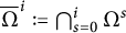 $\overline {\Omega }^i:=\bigcap _{s=0}^{i}\Omega ^s$
, where
 $C^i_j$
’s are given in (12). We mention the difference of
 $\Omega ^i$
with
 $\Delta ^i$
in Theorem 2.
Lemma 5 Let the basic conditions on the system and the homoclinic loop and the assumption
 $(i)$
in Theorem 2 hold. Assume that there exist analytic functions
 $P_i(x,y,\delta )$
and
 $Q_i(x,y,\delta )$
for
 $i=1,2,\ldots ,l,$
such that for
 $\delta \in \overline {\Omega }^{i-1}$
, the equalities (13) hold over U. Then, for
 $\delta \in \overline {\Omega }^{i-1}$
, the conclusions
 $(a)$
–
 $(e)$
of Theorem 2 hold.
Proof Here, we just prove this lemma in the case that the unperturbed system (1)
 $|_{\varepsilon =0}$
has a nilpotent center and a homoclinic loop to a nilpotent cusp. The proof as the homoclinic loop to a nilpotent saddle can be handled in a similar way as that in the proof for the nilpotent cusp.
We first prove the result for
 $l=1$
. Differentiating
 $M^0(h,\delta )$
in the expansions (11) and (12) with respect to h, together with the condition
 $\delta \in \overline {\Omega }^0$
, one has for
 $0<-h\ll 1$
,
 $$ \begin{align} \frac{\partial M^0(h,\delta)}{\partial h}&=B^0_{\frac{k_1+1}{2}}-|h|^{\frac{1}{2}}\sum\limits_{j\geq0}\sum^{k_1j+\frac{k_1-1}{2}}_{r=k_1j+1}\left(\frac{r}{k_1}+\frac{3}{2}\right)B^0_{k_1+r}|h|^{\frac{r}{k_1}}\nonumber\\ &\quad+\sum\limits_{j\geq0}(j+2)B^0_{k_1(j+1)+\frac{k_1+1}{2}}(h-h_s)^{j+1} \nonumber\\ &\quad\quad -|h|^{\frac{1}{2}}\sum\limits_{j\geq0}\sum\limits^{(j+1)k_1-1}_{r=k_1j+\frac{k_1+1}{2}}\left(\frac{r}{k_1}+\frac{3}{2}\right)B^0_{k_1+r+1}|h|^{\frac{r}{k_1}}, \end{align} $$
and for
 $0\leq h-h_c\ll 1$
,
 $$ \begin{align} \frac{\partial M^0(h,\delta)}{\partial h}=(h-h_c)^{\frac{2+k_2}{2k_2}}\sum\limits_{r\geq0}\frac{2+3k_2+4r}{2k_2}C^0_{r+\frac{k_2}{2}}(h-h_c)^{\frac{2r}{k_2}}. \end{align} $$
Set
 $C^1_{r}:=\frac {2+3k_2+4r}{2k_2}C^0_{r+\frac {k_2}{2}}, r\geq 0$
. Recall that the derivative of the first-order Melnikov function
 $M(h,\delta )$
defined by (4) in h has the following expression (see [Reference Han20]):
 $$ \begin{align*} \frac{\partial M(h,\delta)}{\partial h}=\displaystyle\oint_{L^1_h}\left.\left(\frac{\partial P_0}{\partial x}+\frac{\partial Q_0}{\partial y}\right)\right|_{\varepsilon=0}\mathrm{d}t. \end{align*} $$
Substituting equation (13) with
 $i=1$
into the above derivative, a simple computation shows
 $$ \begin{align} \frac{\partial M^0(h,\delta)}{\partial h}=\oint_{L^1_h}Q_1\mathrm{d}x-P_1\mathrm{d}y=:M^1(h,\delta), \end{align} $$
which has the same integral form as the first-order Melnikov function (4). Then, it can be viewed as the first-order Melnikov function
 $M^1(h,\delta )$
of a new near-Hamiltonian system (9) with
 $i=1$
, and it has the expansion (11) near the homoclinic loop and the expansion (12) near the nilpotent center. It follows from equation (2.36) that the expression (2.34) and the expansion (11) with
 $i=1$
are the same near the loop
 $L_s$
, and that the expression (2.35) is consistent with the expansion (12) with
 $i=1$
near the center.
Comparing the coefficients in the expression (2.34) and in the expansion (11) with
 $i=1$
, as well as the coefficients in the expression (2.35) and in (12) with
 $i=1$
, one has for
 $\delta \in \overline {\Omega }^0$
-
(a) when
$r=1,2,\dots ,[\frac {k_1-1}{2}]$
,
$$ \begin{align*} B^1_{k_1j+r}=-\left(\frac{r}{k_1}+\frac{3}{2}+j\right)B^0_{k_1(j+1)+r}, \end{align*} $$
-
(b) when
$r=[\frac {k_1+1}{2}]$
,
$$ \begin{align*} B^1_{k_1j+r}=\left(j+2\right)B^0_{k_1(j+1)+r}, \end{align*} $$
-
(c) when
$r=[\frac {k_1}{2}]+2,\ldots ,k_1$
,
$$ \begin{align*} B^1_{k_1j+r}=-\left(\frac{r-1}{k_1}+\frac{3}{2}+j\right)B^0_{k_1(j+1)+r}, \end{align*} $$
-
(d)
$$ \begin{align*} C^1_j=-\left(\frac{2r+1}{k_2}+\frac{3}{2}\right)C^0_{\frac{k_2}{2}+j}, \end{align*} $$






for all nonnegative integers j. Obviously, the conclusion
 $(e)$
in Theorem 2 holds, which can be obtained from
 $(d)$
above. Taking
 $j=0$
for
 $(a)$
–
 $(c)$
above, one gets the proof of
 $(a)$
,
 $(b),$
and
 $(d)$
in Theorem 2 for
 $l=1$
.
For
 $l>1$
, according to the foregoing proof and the conditions of Lemma 5, for
 $\delta \in \overline {\Omega }^{i-1}$
, the conclusions
 $(a)$
–
 $(d)$
hold with the superscripts i and
 $i-1$
instead of the superscripts
 $1$
and
 $0$
, respectively.
By induction, one can further prove that for
 $\delta \in \overline {\Omega }^{i-1}$
,
-
(a) when
$r=1,2,\dots ,[\frac {k_1-1}{2}]$
,
$$ \begin{align*} B^0_{k_1(i+j)+r}=\frac{(-1)^i(2k_1)^i}{\prod\limits_{s=j+1}^{i+j}\left(k_1+2(k_1s+r)\right)}B^i_{k_1j+r}, \end{align*} $$
-
(b) when
$r=[\frac {k_1+1}{2}]$
,
$$ \begin{align*} B^0_{k_1(i+j)+r}=\frac{1}{\prod\limits_{s=j+2}^{i+j+1}s}B^i_{k_1j+r}, \end{align*} $$
-
(c) when
$r=[\frac {k_1}{2}]+2,\ldots ,k_1$
,
$$ \begin{align*} B^0_{k_1(i+j)+r}=\frac{(-1)^i(2k_1)^i}{\prod\limits_{s=j+1}^{i+j}\left(k_1+2(k_1s+r-1)\right)}B^i_{k_1j+r}, \end{align*} $$
-
(d)
$$ \begin{align*} C^0_{\frac{k_2}{2}i+j}=\frac{(2k_2)^i}{\prod\limits^i_{s=1}((2s+1)k_2+4j+2)}C^i_{j}, \end{align*} $$






with nonnegative integers j.
Statement
 $(d)$
above implies the conclusion
 $(e)$
in Theorem 2. Taking
 $j=0$
in the above conclusions
 $(a)$
–
 $(c)$
, it follows the conclusions
 $(a)$
,
 $(b),$
and
 $(d)$
in Theorem 2. The proof is completed.
Proof of Theorem 2
It follows from Lemma 5, together with the fact
 $\overline {\Delta }^{i-1}\subseteq \overline {\Omega }^{i-1}$
for
 $i=1,2,\ldots ,l$
.
Next, we turn to think about the coefficients of the terms with higher degrees in the expansion of the first-order Melnikov function near the homoclinic loop to the nilpotent cusp, called a cuspidal loop. Han et al. [Reference Han, Zang and Yang27] first depicted the expansions of the first-order Melnikov function near this kind of loop, and the first coefficients in the expansions for
 $k=3$
. In [Reference Atabaigi, Zangeneh and Kazemi3, Reference Wei and Zhang52, Reference Xiong56] the authors further studied the coefficients with lower degrees of the expansions for
 $k\geq 5$
. The results are summarized as follows.
Lemma 6 For the analytic near-Hamiltonian system (9), assume that the unperturbed Hamiltonian has an oriented clockwise homoclinic loop to a nilpotent cusp at the origin, and satisfies (2) with
 $h_k<0$
, then the first-order Melnikov function near and inside the cuspidal loop is given in (11), and it near and outside the loop
 $($
see Figure 1
 $(A))$
can be written in the form
 $$ \begin{align} M^i(h,\delta)&=b^i_0+\sum\limits_{j\geq0}\sum^{kj+\frac{k-1}{2}}_{r=kj+1}b^i_{r}h^{\frac{r}{k}+\frac{1}{2}}+\sum\limits_{j\geq0}b^i_{kj+\frac{k+1}{2}}h^{j+1} \nonumber\\ &\qquad\qquad +\sum\limits_{j\geq0}\sum\limits^{(j+1)k-1}_{r=kj+\frac{k+1}{2}}b^i_{r+1}h^{\frac{r}{k}+\frac{1}{2}}. \qquad 0<h\ll1, \end{align} $$
where
 $$ \begin{align} \begin{aligned} &b^i_0=B^i_0,\qquad\qquad\qquad\qquad\ \ b^i_{r}=\frac{A^*_{r-1}}{A_{r-1}}B^i_r,\quad r=1,\dots,\left[\frac{k}{2}\right], \\ &b^i_{[\frac{k}{2}]+1}=B^i_{[\frac{k}{2}]+1}+\sum\limits_{l=1}^{\left[\frac{k}{2}\right]}T^*_lB^i_l,\quad b^i_{r}=\frac{A^*_{r-2}}{A_{r-2}}B^i_r,\quad r=\left[\frac{k}{2}\right]+2,\ldots,k, \end{aligned} \end{align} $$
with the constants
 $T^*_l$
,
 $A^*_r>0$
for
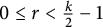 $0\leq r<\frac {k}{2}-1$
and
 $A^*_r<0$
, for
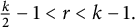 $\frac {k}{2}-1<r<k-1.$
Yang and Han [Reference Yang and Han62] in 2024 provided further the relation between the coefficients of the terms with the same order in the asymptotic expansions of the first-order Melnikov functions inside or outside the cuspidal loop. Moreover, the constants
 $T^*_l$
’s are zeros in Lemma 6.
This lemma implies the information
 $$\begin{align*}\left\{\delta: B^i_r(\delta)=0, 1\leq r\leq k, r\neq \left[\frac{k}{2}\right]+1\right\}=\left\{\delta: b^i_r(\delta)=0, 1\leq r\leq k, r\neq \left[\frac{k}{2}\right]+1\right\}. \end{align*}$$
In the light of the idea in Theorem 2 and its proof, together with this last lemma, we can characterize the coefficients of the expansions (11) and (2.37) of the first-order Melnikov functions near the cuspidal loop, as shown in the next results. Their proofs will be omitted.
Theorem 7 For the analytic near-Hamiltonian system (1), the following assumptions hold:
-
(i) The unperturbed Hamiltonian one of system (1) has a nilpotent center of order
$\left [\frac {k_2}{2}\right ]-1$
and an oriented clockwise homoclinic loop to a nilpotent cusp of order
$\left [\frac {k_1-1}{2}\right ]$
. -
(ii) The first-order Melnikov function is of the form (11) with
$i=0$
near the loop, and is of the form (12) with
$i=0$
near the center. -
(iii) There exist analytic functions
$P_i(x,y,\delta )$
and
$Q_i(x,y,\delta )$
for
$i=1,2,\ldots ,l,$
such that for
$\delta \in \overline {\Delta }^{i-1}$
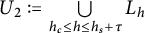
, the equations (13) hold over
$U_2:=\bigcup \limits _{h_c\leq h\leq h_s+\tau }L_h$
with a positive number
$\tau \ll 1$
.





Then, the statements
 $(a)$
,
 $(b)$
,
 $(d),$
and
 $(e)$
in Theorem 2 hold, and the coefficients of the expansions have the next relations.
-
(a) For
$r=1,2,\dots ,\frac {k_1-1}{2}$
,
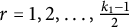
$$ \begin{align*} b^0_{k_1i+r}\Big|_{\overline{\Delta}^{i-1}}=\frac{(2k_1)^i}{\prod\limits^i_{j=1}((2j+1)k_1+2r)}b^i_r. \end{align*} $$
-
(b) For
$r=\frac {k_1+1}{2}$
,
$$ \begin{align*} b^0_{k_1i+r}\Big|_{\overline{\Delta}^{i-1}}=\frac{1}{(i+1)!}b^i_r. \end{align*} $$
-
(c) For
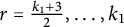
$r=\frac {k_1+3}{2},\ldots ,k_1$
,
$$ \begin{align*} b^0_{k_1i+r}\Big|_{\overline{\Delta}^{i-1}}=\frac{(2k_1)^i}{\prod\limits^i_{j=1}((2j+1)k_1+2r-2)}b^i_r. \end{align*} $$



3 Limit cycle bifurcations near a homoclinic loop and a center
This section considers the limit cycle bifurcations of the families of periodic orbits near a center and a homoclinic loop with a nilpotent singularity. If the singularity is a nilpotent saddle, the Hamiltonian system (1)
 $|_{\varepsilon =0}$
could have a family of periodic orbits either inside or outside the homoclinic loop. If the singularity is a nilpotent cusp, there could have two families of periodic orbits locating at both sides of the cuspidal loop (see Figure 1(A)). In this last case, we study limit cycle bifurcations in both sides of the cuspidal loop and near the center for the near-Hamiltonian system (1), utilizing the properties of the coefficients of the first-order Melnikov functions estabilished in Theorems 2 and 3 and Lemma 7. On the limit cycle bifurcation in a single side of a homoclinic loop and near a nilpotent center will be directly demonstrated without a proof, since they can be obtained in a similar way as that in the case of the cuspidal loop.
Set
 $B_0:=B^0_0$
. For
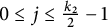 $0\leq j\leq \frac {k_2}{2}-1$
,
 $1\leq r\leq k_1$
and
 $r\neq [\frac {k_1}{2}]+1$
, set
 $$ \begin{align} C_{\frac{k_2}{2}i+j}:= \begin{cases} C^0_j,&\quad i=0,\\ C^0_{\frac{k_2}{2}i+j}\big|_{\overline{\Delta}^{i-1}},&\quad i>0, \end{cases}\qquad B_{k_1i+r}:= \begin{cases} B^0_{r},&\quad i=0,\\ B^0_{k_1i+r}|_{\overline{\Delta}^{i-1}},&\quad i>0. \end{cases} \end{align} $$
For
 $r=[\frac {k_1}{2}]+1$
, set

Denote
 $$ \begin{align*} &\mathbf{F}^i:=\left(C^i_{11},C^i_{21},\ldots,C^i_{\frac{k_2}{2}-1,1}\right),\qquad \mathbf{F}_i:=(\mathbf{F}^0,\mathbf{F}^1,\ldots,\mathbf{F}^i),\qquad \mathbf{F}_{-1}:=\varnothing,\\ &\mathbf{A}^i:=\left(B^i_{1},B^i_{2},\ldots,B^i_{[\frac{k_1}{2}]},B^i_{[\frac{k_1}{2}]+2},\ldots,B^i_{k_1},C^i_0,C^i_1,\ldots,C^i_{\frac{k_2}{2}-1}\right),\\ &\mathbf{A}_i:=\left(B_{k_1i+1},B_{k_1i+2},\ldots,B_{k_1i+[\frac{k_1}{2}]},B_{k_1i+[\frac{k_1}{2}]+2},\ldots,B_{k_1i+k_1},C_{\frac{k_2}{2}i},\ldots,C_{\frac{k_2}{2}(i+1)-1}\right),\\ &O_i:=O\left(\big|B_{k_1i+1},B_{k_1i+2},\ldots,B_{k_1i+[\frac{k_1}{2}]}\big|\right), \end{align*} $$
and
 $$ \begin{align*} &O^j:=\begin{cases} O(|\mathbf{A}_0,\mathbf{A}_1,\ldots,\mathbf{A}_{j-1},\mathbf{F}_{j-1}|),&j>0,\\ 0,&j=0. \end{cases} \end{align*} $$
Theorem 8 Let assumptions
 $(i)$
and
 $(ii)$
in Theorem 7 hold. If there exist nonnegative integers
 $n(\leq m)$
,
 $r_1\in [1,k_1], r_2\in [0,\frac {k_2}{2}-1]$
and
 $\delta _0\in \mathbb {R}^{d}$
, such that for
 $B_j$
and
 $C_j$
defined in (39) and (40),
 $$ \begin{align*} & B_{k_1n+r_1}(\delta_{0})C_{\frac{k_2}{2}n+r_2}(\delta_{0})\neq 0,\qquad\qquad \mathbf{F}_{n-1}(\delta_0)= \mathbf{0},\\ & B_i(\delta_{0} )=C_j(\delta_{0} )=0,\quad i=0,1,\ldots,k_1n+r_1-1,~j=0,1,\dots,\frac{k_2}{2}n+r_2-1, \\ & \mathrm{Rank} \frac{\partial\left(B_{0},B_1,\ldots,B_{k_1n+r_1-1},C_{0},\ldots,C_{\frac{k_2}{2}n+r_2-1},\mathbf{F}_{n-1}\right)}{\partial(\delta_{1},\ldots,\delta_{s})}(\delta_{0} )=(k_1+k_2-1)n+r_1+r_2. \end{align*} $$
Then, system (1) can have
 $(2k_1+\frac {k_2}{2}-1)n+2r_1+r_2-1$
limit cycles near either the center or the cuspidal loop for some
 $(\varepsilon ,\delta )$
near
 $(0,\delta _0)$
, being composed of
 $(2k_1-1)n+2r_1-1$
limit cycles near the cuspidal loop and
 $\frac {k_2}{2}n+r_2$
limit cycles near the center.
Proof Without loss of generality, we assume that
 $(-1)^{k_1n+r_1} B_{k_1n+r_1}(\delta _0)>0$
for
 $r_1<\frac {k_1+3}{2}$
and
 $(-1)^{\frac {k_2}{2}n+r_2}C_{\frac {k_2}{2}n+r_2}(\delta _0)>0$
. For unifying the notations, we denote by
 $B^i_{jl}:=B^i_j$
for
 $l=1$
and
 $B^i_{jl}:=b^i_j$
for
 $l=2$
. It follows from the expansion (11) and Lemma 6 that the asymptotic expansions of the first-order Melnikov function near the cuspidal loop can be uniformly written in
 $$ \begin{align} M_l^0(h,\delta)=&B^0_{0l}+|h|^{\frac{1}{2}}\sum\limits_{j\geq0}\sum^{k_1j+\frac{k_1-1}{2}}_{r=k_1j+1}B^0_{rl}|h|^{\frac{r}{k_1}}+\sum\limits_{j\geq0}B^0_{k_1j+\frac{k_1+1}{2},l}h^{j+1} \nonumber\\ &\qquad +|h|^{\frac{1}{2}}\sum\limits_{j\geq0}\sum\limits^{(j+1)k_1-1}_{r=k_1j+\frac{k_1+1}{2}}B^0_{r+1,l}|h|^{\frac{r}{k_1}} \end{align} $$
for
 $0<(-1)^lh\ll 1$
with
 $l\in \{1,2\}$
, and that the asymptotic expansion near the center is given in (12) with
 $i=0$
.
To study the number of isolated zeros of the first-order Melnikov function, treating
 $B_i, C_{j}$
and
 $\mathbf {F}_{n-1}$
with
 $i=0,1,\ldots ,k_1n+r_1-1, j=0,1,\dots ,\frac {k_2}{2}n+r_2-1$
as free parameters, and write
 $B^0_{il}$
’s and
 $C^0_i$
’s in terms of
 $B_i$
’s and
 $C_i$
’s. Then,
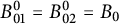 $B^0_{01}=B^0_{02}=B_{0}$
,
 $C^0_0=C_0$
, and
 $$ \begin{align*} B^0_{k_1j+r,l}&=\left.B^0_{k_1j+r,l}\right|_{\overline{\Delta}^{j-1}}+O\left(|\mathbf{A}^0,\mathbf{A}^1,\ldots,\mathbf{A}^{j-1},\mathbf{F}^0,\mathbf{F}^1,\ldots,\mathbf{F}^{j-1}|\right)\\&=\left.B^0_{k_1j+r,l}\right|_{\overline{\Delta}^{j-1}}+O^j,\\ C^0_{\frac{k_2}{2}j+t}&=\left. C^0_{\frac{k_2}{2}j+t}\right|_{\overline{\Delta}^{j-1}}+O^j. \end{align*} $$
Together with the properties in Theorem 7 and the relations (2.38), one further has
 $$ \begin{align*} B^0_{k_1j+r,l}= \begin{cases} B_{k_1j+r}+O^j,&l=1,\\ (-1)^{j}\frac{A^*_{r-1}}{A_{r-1}}B_{k_1j+r}+O^j,&l=2 \end{cases} \end{align*} $$
for
 $1\leq r\leq [\frac {k_1}{2}]$
,
 $$ \begin{align*} B^0_{k_1j+r,l}=B_{k_1j+r}+O_j+O^j \end{align*} $$
for
 $r=[\frac {k_1}{2}]+1$
,
 $$ \begin{align*} B^0_{k_1j+r,l}= \begin{cases} B_{k_1j+r}+O^j,&l=1,\\ (-1)^{j}\frac{A^*_{r-2}}{A_{r-2}}B_{k_1j+r}+O^j,&l=2 \end{cases} \end{align*} $$
for
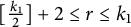 $[\frac {k_1}{2}]+2\leq r\leq k_1$
, and
 $$ \begin{align*} C^0_{\frac{k_2}{2}j+t}=C_{\frac{k_2}{2}j+t}+O^j \end{align*} $$
for
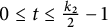 $0\leq t\leq \frac {k_2}{2}-1$
.
Therefore, the expansions (41) of the first-order Melnikov function can be, respectively, written in
 $$ \begin{align*} M_1^0(h,\delta)&=B_0+\sum\limits_{j=0}^{n-1}\sum^{k_1j+\frac{k_1-1}{2}}_{r=k_1j+1}\left(B_r+O^j\right)|h|^{\frac{r}{k_1}+\frac{1}{2}}+ \sum\limits^{n-1}_{j=0}\left((-1)^{j+1}B_{k_1j+\frac{k_1+1}{2}}+O_j+O^j\right)\notag\\ & \qquad\cdot|h|^{j+1}+\sum\limits_{j=0}^{n-1}\sum\limits^{(j+1)k_1-1}_{r=k_1j+\frac{k_1+1}{2}}\left(B_{r+1}+O_j\right)|h|^{\frac{r}{k_1}+\frac{1}{2}} +\sum\limits^{k_1n+r_1-1}_{r=k_1n+1}\left(B_{r}+O^n\right)\\ & \qquad\quad\cdot|h|^{\frac{r}{k_1}+\frac{1}{2}}+B^0_{k_1n+r_1}|h|^{n+\frac{r_1}{k_1}+\frac{1}{2}}+o\left(|h|^{n+\frac{r_1}{k_1}+\frac{1}{2}}\right)\notag \end{align*} $$
near and inside the loop
 $L_s$
,
 $$ \begin{align*} M^0_2(h,\delta)&=B_0+\sum\limits_{j=0}^{n-1}\sum^{k_1j+\frac{k_1-1}{2}}_{r=k_1j+1}\left((-1)^{j+1}\left|\frac{A^*_{r-1}}{A_{r-1}}\right|B_r+O^j\right)h^{\frac{r}{k_1}+\frac{1}{2}}+\sum\limits^{n-1}_{j=0}\left(B_{k_1j+\frac{k_1+1}{2}}\right.\notag\\ & \qquad\left.+O_j+O^j\right)h^{j+1}+\sum\limits_{j=0}^{n-1}\sum\limits^{(j+1)k_1-1}_{r=k_1j+\frac{k_1+1}{2}}\left((-1)^{j+1}\left|\frac{A^*_{r-1}}{A_{r-1}}\right|B_{r+1}+O^j\right)\cdot h^{\frac{r}{k_1}+\frac{1}{2}}\\ & \qquad\qquad +\sum\limits^{k_1n+r_1-1}_{r=k_1n+1}\left((-1)^{n+1}\left|\frac{A^*_{r-1}}{A_{r-1}}\right|B_{r}+O^n\right)h^{\frac{r}{k_1}+\frac{1}{2}}\notag\\ & \qquad\qquad\qquad+b^0_{k_1n+r_1}h^{n+\frac{r_1}{k_1}+\frac{1}{2}}+o\left(h^{n+\frac{r_1}{k_1}+\frac{1}{2}}\right) \notag \end{align*} $$
near and outside the loop, and
 $$ \begin{align*} M^0(h,\delta)&=(h-h_c)^{\frac{k_2+2}{2k_2}}\left(\sum\limits^{n-1}_{j=0}\sum\limits^{\frac{k_2}{2}(j+1)-1}_{r=\frac{k_2}{2}j}\left(C_r+O^j\right) (h-h_c)^{\frac{2r}{k_2}}+\sum\limits^{\frac{k_2}{2}n+r_2-1}_{r=\frac{k_2}{2}n}\left(C_r+O^n\right) \right.\notag\\ &\quad\left. \phantom{\sum\limits^{n-1}_{j=0}}(h-h_c)^{\frac{2r}{k_2}}+C^0_{\frac{k_2}{2}n+r_2}(h-h_c)^{1+\frac{2n+r_2}{k_2}}+o\left(|h-h_c|^{1+\frac{2n+r_2}{k_2}}\right)\right) \end{align*} $$
near the nilpotent center for
 $0<h-h_c\ll 1,$
where
 $B^0_{k_1n+r_1}=B_{k_1n+r_1}(\delta _0)+\overline {O},~b^0_{k_1n+r_1}=(-1)^n\frac {A^*_{k_1n+r_1-2}}{A_{k_1n+r_1-2}}B_{k_1n+r_1}(\delta _0)+\overline {O}$
, and
 $C^0_{\frac {k_2}{2}n+r_2}=C_{\frac {k_2}{2}n+r_2}(\delta _0)+\overline {O}$
with
 $\overline {O}=O(|B_{0},B_{1},\ldots , B_{k_1n+r_1-1},C_0,C_1,\ldots ,C_{\frac {k_2}{2}n+r_2-1},\mathbf {F}_{n-1}|)$
. Take the free parameters
 $B_i$
’s and
 $C_i$
’s such that
 $$ \begin{align*} 0<&(-1)^{k_1j}B_{k_1j}\ll (-1)^{k_1j+1}B_{k_1j+1}\ll\cdots\ll(-1)^{k_1j+\frac{k_1-1}{2}}B_{k_1j+\frac{k_1-1}{2}}\ll\\ & (-1)^{k_1j+\frac{k_1-1}{2}+j}B_{k_1j+\frac{k_1+1}{2}}\ll (-1)^{k_1j+\frac{k_1+3}{2}}B_{k_1j+\frac{k_1+3}{2}}\ll \cdots\ll (-1)^{k_1j+k_1}B_{k_1j+k_1}\\ &\ll(-1)^{k_1n+1}B_{k_1n+1}\ll\cdots\ll(-1)^{k_1n+r_1-1}B_{k_1n+r_1-1}\ll(-1)^{k_1n+r_1}B_{k_1n+r_1}(\delta_0),\\ 0<&(-1)^{r-1}C_{r-1}\ll (-1)^{r}C_{r}\ll(-1)^{\frac{k_2}{2}n+r_2}C_{\frac{k_2}{2}n+r_2}(\delta_0) \end{align*} $$
satisfying
 $\mathrm {max}\left \{|B_{k_1(j+1)}|,|C_{\frac {k_2}{2}j+\frac {k_2}{2}-1}|\right \}\ll \mathrm {min}\left \{|B_{k_1(j+1)+1}|,|C_{\frac {k_2}{2}(j+1)}|\right \}$
with
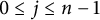 $0\leq j\leq n-1$
and
 $1\leq r\leq \frac {k_2}{2}n+r_2-1$
. Then, the first-order Melnikov function
 $M(h,\delta )$
can have
 $k_1n+r_1$
simple zeros in a right neighborhood of
 $h=0$
and
 $(k_1-1)n+r_1-1$
simple zeros in a left neighborhood of
 $h=0$
, and
 $\frac {k_2}{2}n+r_2$
simple zeros near
 $h=h_c$
. Hence, the near-Hamiltonian system (1) can have
 $(2k_1+\frac {k_2}{2}-1)n+2r_1+r_2-1$
limit cycles near either the cuspidal loop or the nilpotent center, obtained by applying the implicit function theorem to the Poincaré map.
The proofs of the other cases are similar as those given above, and so are omitted. We finish the proof of the theorem.
We remark that in practice, it is quite troublesome to find
 $\delta _0$
that meets the conditions in Theorem 8. If the perturbations
 $P_0$
and
 $Q_0$
in system (1) are linear in the parameter
 $\delta $
, the Jacobian matrix in the theorem is independent of the parameter
 $\delta $
. Then, we can simplify the conditions in Theorem 8 even further.
Corollary 1 Let assumptions
 $(i)$
and
 $(ii)$
in Theorem 7 hold. Suppose that there exist nonnegative integers
 $n(\leq m)$
,
 $r_1\in [1,k_1]$
and
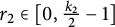 $r_2\in [0,\frac {k_2}{2}-1]$
, such that the Jacobian matrix
 $$\begin{align*}\frac{\partial\left(B_{0},B_1,\ldots,B_{k_1n+r_1-1},C_{0},\ldots,C_{\frac{k_2}{2}n+r_2-1},\mathbf{F}_{n-1},b\right)}{\partial(\delta_{1},\ldots,\delta_{s})} \end{align*}$$
with
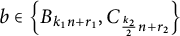 $b\in \left \{B_{k_1n+r_1},C_{\frac {k_2}{2}n+r_2}\right \}$
is of full rank. Then, system (1) can have
 $(2k_1+\frac {k_2}{2}-1)n+2r_1+r_2-1$
limit cycles near either the nilpotent center or the cuspidal loop for suitable choices of the values of
 $(\varepsilon ,\delta )$
.
Based on the ideas in the proof of Theorem 8, one can establish similar results on limit cycle bifurcations near and inside a homoclinic loop to a nilpotent singularity and near a nilpotent center. We present them here without a proof, because of the similarity and cumbersome.
Theorem 9 Let assumptions
 $(i)$
and
 $(ii)$
in Theorem 2 hold. Suppose that there exist nonnegative integers
 $n(\leq m)$
,
 $r_1\in [1,k_1], r_2\in [0,\frac {k_2}{2}-1]$
and
 $\delta _0\in \mathbb {R}^{s}$
, such that the
 $B_j$
’s and
 $C_j$
’s defined in (39) and (40) satisfy the following conditions:
 $$ \begin{align*} & B_{k_1n+r_1}(\delta_{0})C_{\frac{k_2}{2}n+r_2}(\delta_{0})\neq 0,\qquad\qquad \mathbf{F}_{n-1}(\delta_0)= \mathbf{0},\\ & B_i(\delta_{0} )=C_{j}(\delta_{0} )=0,\quad i=0,1,\ldots,k_1n+r_1-1,~j=0,1,\dots,\frac{k_2}{2}n+r_2-1, \\ & \mathrm{Rank} \frac{\partial\left(B_{0},B_1,\ldots,B_{k_1n+r_1-1},C_{0},\ldots,C_{\frac{k_2}{2}n+r_2-1},\mathbf{F}_{n-1}\right)}{\partial(\delta_{1},\ldots,\delta_{s})}(\delta_{0} )=(k_1+k_2-1)n+r_1+r_2. \end{align*} $$
Then, system (1) can have
 $(k_1+\frac {k_2}{2})n+r_1+r_2$
limit cycles near either the center or the homoclinic loop for suitable choices of the values of
 $(\varepsilon ,\delta )$
near
 $(0,\delta _0)$
.
Corollary 2 Let assumptions
 $(i)$
and
 $(ii)$
in Theorem 2 hold. If there exist nonnegative integers
 $n(\leq m)$
,
 $r_1\in [1,k_1],$
and
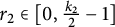 $r_2\in [0,\frac {k_2}{2}-1]$
, such that the Jacobian matrix
 $$\begin{align*}\frac{\partial\left(B_{0},B_1,\ldots,B_{k_1n+r_1-1},C_{0},\ldots,C_{\frac{k_2}{2}n+r_2-1},\mathbf{F}_{n-1},b\right)}{\partial(\delta_{1},\ldots,\delta_{s})} \end{align*}$$
with
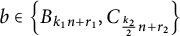 $b\in \left \{B_{k_1n+r_1},C_{\frac {k_2}{2}n+r_2}\right \}$
is of full rank. Then, system (1) can have
 $(k_1+\frac {k_2}{2})n+r_1+r_2$
limit cycles near either the center or the homoclinic loop for suitable choices of the values of
 $(\varepsilon ,\delta )$
near
 $(0,\delta _0)$
.
For
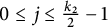 $0\leq j\leq \frac {k_2}{2}-1$
, set
 $$ \begin{align} C_{\frac{k_2}{2}i+j}:= \begin{cases} C^0_j,&\quad i=0,\\ C^0_{\frac{k_2}{2}i+j}|_{\overline{\Lambda}^{i-1}},&\quad i>0. \end{cases} \end{align} $$
Theorem 10 Let assumptions
 $(i)$
and
 $(ii)$
in Theorem 3 hold. Suppose that there exist nonnegative integers
 $n(\leq m)$
,
 $r(\leq \frac {k_2}{2}-1),$
and
 $\delta _0\in \mathbb {R}^{s}$
, such that the
 $C_j$
’s defined in (40) satisfy
 $$ \begin{align*} & C_{\frac{k_2}{2}n+r}(\delta_{0})\neq 0,\qquad\qquad \mathbf{F}_{n-1}(\delta_0)= \mathbf{0},\\ & C_{l}(\delta_{0} )=0,\quad l=0,1,\dots,\frac{k_2}{2}n+r-1, \\ & \mathrm{Rank} \frac{\partial\left(C_{0},\ldots,C_{\frac{k_2}{2}n+r-1},\mathbf{F}_{n-1}\right)}{\partial(\delta_{1},\ldots,\delta_{s})}(\delta_{0} )=(k_2-1)n+r. \end{align*} $$
Then, system (1) can have
 $\frac {k_2}{2}n+r$
limit cycles near the center for suitable choices of the values of
 $(\varepsilon ,\delta )$
near
 $(0,\delta _0)$
.
Corollary 3 Let assumptions
 $(i)$
and
 $(ii)$
in Theorem 3 hold. If there exist nonnegative integers
 $n(\leq m)$
and
 $r(\leq \frac {k_2}{2}-1)$
, such that the Jacobian matrix
 $$\begin{align*}\frac{\partial\left(C_{0},\ldots,C_{\frac{k_2}{2}n+r-1},\mathbf{F}_{n-1},C_{\frac{k_2}{2}n+r}\right)}{\partial(\delta_{1},\ldots,\delta_{s})} \end{align*}$$
is of full rank, then system (1) can have
 $\frac {k_2}{2}n+r$
limit cycles near the center for some
 $(\varepsilon ,\delta )$
.
Denoted by
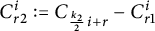 $C^i_{r2}:=C_{\frac {k_2}{2}i+r}-C^i_{r1}$
,
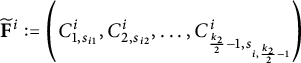 $\widetilde {\mathbf {F}}^i:=\left (C^i_{1,s_{i1}},C^i_{2,s_{i2}},\ldots , C^i_{\frac {k_2}{2}-1,s_{i,\frac {k_2}{2}-1}}\right )$
,
 $\widetilde {\mathbf {F}}_i:=\left (\widetilde {\mathbf {F}}^0, \right. \left. \widetilde {\mathbf {F}}^1,\ldots , \widetilde {\mathbf {F}}^i\right )$
for
 $i\geq 0$
and
 $\widetilde {\mathbf {F}}_{-1}=\varnothing $
.
We remark that if there exists a maximal linearly independent group
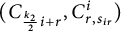 $(C_{\frac {k_2}{2}i+r},C^i_{r,s_{ir}})$
with
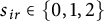 $s_{ir}\in \{0,1,2\}$
, where
 $C^i_{r0}=\varnothing $
, then Theorems 8–10 and Corollaries 1–3 still hold with the symbol
 $\widetilde {\mathbf {F}}$
instead of the symbol
 $\mathbf {F}$
.
4 Applications
This section is a proof of Theorems 5 and 6, which are the applications of our results obtained in the previous sections to two concrete systems.
4.1 Proof of Theorem 5
Consider the generalized Liénard system of the form:
 $$ \begin{align} \dot x=y,\qquad \dot y=-x^2(x-1)^3+\varepsilon yf_m(x). \end{align} $$
with a polynomial
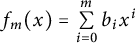 $f_m(x)=\sum \limits ^m_{i=0}b_{i}x^i$
. Obviously, the Hamiltonian of the unperturbed system (43)
 $|_{\varepsilon =0}$
is
 $H(x,y)=\frac {1}{2}y^{2}-\frac {1}{3}x^{3}+\frac {3}{4}x^{4}-\frac {3}{5}x^5+\frac {1}{6}x^6$
, and its associated system has a nilpotent center of order 1 at the point
 $(1,0)$
and a cuspidal loop
 $L_s$
, which is contained in the level set
 $H(x,y)=0$
and is homoclinic to the cusp of order 1 at the origin. By Theorem 1, the coefficients of the first-order Melnikov function (11) with
 $i=0$
and (2.33) satisfy
 $$ \begin{align} B_{0}&=\sum\limits^m_{i=0}b_iI_i,&C_{0}&=2\mathrm{B}\left(\frac{1}{4},\frac{3}{2}\right)\sum\limits^m_{i=0}b_{i},&\nonumber\\ B_{1}&=2^{\frac{3}{2}}3^{\frac{1}{3}}A_0b_{0},&C_{1}&=2\mathrm{B}\left(\frac{3}{4},\frac{3}{2}\right)\sum\limits^m_{i=0}\left(i^2+\frac{1}{5}i+\frac{41}{25}\right)b_{i},&\\ B_{2}&=\sum\limits^m_{i=1}b_iJ_i,& C^0_{11}&=2\mathrm{B}\left(\frac{3}{4},\frac{3}{2}\right)\sum\limits^m_{i=0}\left(i(i-1)+\frac{41}{25}\right)b_{i},& \nonumber\\ B_{3}&=2^{\frac{1}{2}}3^{\frac{2}{3}}A_1(3b_{0}+2b_{1}),& & \nonumber \end{align} $$
where the constants
 $A_0, A_1$
are given in Lemma 2, and
 $$ \begin{align*} &I_i=\oint_{L_s}yx^i\mathrm{d}x=2\sqrt{2}\int\limits_0^{x_0}x^{i+1}\sqrt{\frac{1}{3}x-\frac{3}{4}x^2+\frac{3}{5}x^3-\frac{1}{6}x^4}\mathrm{d}x,&\quad& i=0,1,\ldots,m,\\ & J_i=\oint_{L_s}x^i\mathrm{d}t=\sqrt{2}\int\limits_0^{x_0}\frac{x^{i-1}}{\sqrt{\frac{1}{3}x-\frac{3}{4}x^2+\frac{3}{5}x^3-\frac{1}{6}x^4}}\mathrm{d}x,&\quad& i=1,2,\ldots,m,\nonumber \end{align*} $$
with
 $x_0=\frac {(28+10\sqrt {10})^{\frac {1}{3}}}{10}-\frac {3}{5(28+10\sqrt {10})^{\frac {1}{3}}}+\frac {6}{5}$
. Write the expressions (44) in the compact form
 $$ \begin{align} (B_0,B_1,B_2,B_3,C_0,C_1,C^0_{11})^T=R_0(b_{0},b_{1},\ldots,b_{m})^T, \end{align} $$
with
 $R_0$
a
 $7\times (m+1)$
matrix of the form
 $$ \begin{align*} R_0= \begin{pmatrix} I_0 & I_1 & I_2 & \cdots & I_m \\ 2^{\frac{3}{2}}3^{\frac{1}{3}}A_0 & 0 & 0 & \cdots & 0 \\ 0 & J_1 & J_2 & \cdots & J_m \\ 2^{\frac{1}{2}}3^{\frac{5}{3}}A_1 & 2^{\frac{3}{2}}3^{\frac{2}{3}}A_1 & 0 & \cdots & 0 \\ 2\mathrm{B}(\frac{1}{4},\frac{3}{2}) & 2\mathrm{B}(\frac{1}{4},\frac{3}{2}) & 2\mathrm{B}(\frac{1}{4},\frac{3}{2}) & \cdots &2\mathrm{B}(\frac{1}{4},\frac{3}{2})\\ 2\mathrm{B}(\frac{3}{4},\frac{3}{2})\cdot\frac{41}{25} & 2\mathrm{B}(\frac{3}{4},\frac{3}{2})\cdot\frac{71}{25} & 2\mathrm{B}(\frac{3}{4},\frac{3}{2})\cdot\frac{151}{25}& \cdots &2\mathrm{B}(\frac{3}{4},\frac{3}{2})\cdot\left(m^2+\frac{1}{5}m+\frac{41}{25}\right)\\ 2\mathrm{B}(\frac{3}{4},\frac{3}{2})\cdot\frac{41}{25} & 2\mathrm{B}(\frac{3}{4},\frac{3}{2})\cdot\frac{41}{25} & 2\mathrm{B}(\frac{3}{4},\frac{3}{2})\cdot\frac{91}{25}& \cdots &2\mathrm{B}(\frac{3}{4},\frac{3}{2})\cdot\left(m(m-1)+\frac{41}{25}\right) \end{pmatrix}. \end{align*} $$
The condition
 $\overline {\Delta }^0=\Delta ^0$
in Theorem 2 yields
 $x^2|f_m(x)$
and
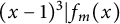 $(x-1)^3|f_m(x)$
. It follows from
 $$\begin{align*}P_0=0\quad \text{and}\quad Q_0=yf_m(x) \end{align*}$$
that equation (13) with
 $i=1$
holds by ordering
 $$ \begin{align*}P_1=\frac{f_m(x)|_{\overline{\Delta}^0}}{x^2(x-1)^3},\end{align*} $$
which implies the expression
 $$ \begin{align*}P_1=\sum\limits^{m-5}_{j=0}b^1_jx^j,\end{align*} $$
where
 $$ \begin{align*}b^1_j=\sum\limits^{m-j}_{l=5}\frac{(l-3)(l-4)}{2}b_{l+j}\quad \text{for}\quad j=0,1,2,\ldots,m-5.\end{align*} $$
Set
 $$ \begin{align*}P_{i-1}:=\sum\limits^{n_{i-1}}_{j=0}b^{i-1}_jx^j \quad\text{and}\quad Q_{i-1}:=0,\end{align*} $$
with
 $n_{i-1}=m+1-6(i-1)$
for
 $i\geq 2.$
Manipulating as the above paragraph, it follows from the condition
 $\overline {\Delta }^i$
and the equality (13) that
 $$ \begin{align*}P_i=\sum\limits^{n_i}_{j=0}b^i_jx^j\quad \text{and}\quad Q_i=0,\end{align*} $$
where
 $$ \begin{align*}b^i_j=\sum\limits^{n_i-j+6}_{l=6}\frac{(l-4)(l-5)}{2}(l+j)b^{i-1}_{l+j}\end{align*} $$
for
 $j=0,1,2,\ldots ,n_i$
and
 $n_i=n_{i-1}-6=m+1-6i$
.
Moreover, one has the next relations on the coefficients
 $$ \begin{align} (b^i_{1},b^i_{2},\ldots,b^i_{m-6i+1})^T=\prod\limits^{i}_{j=1}A^i_j(b_{6i},b_{6i+1},\ldots,b_{m})^T, \quad i=1,2,\dots,\left[\frac{m-1}{6}\right] \end{align} $$
with
 $A^i_j$
being the upper triangular matrices of order
 $m-6i+1$
 $$ \begin{align*} A^i_j&=\begin{pmatrix} 1\cdot(6j+1) & 3\cdot(6j+2) & \cdots & (m-6(i-j)+1)\cdot\frac{(m-6i+2)(m-6i+1)}{2} \\ 0 & 1\cdot(6j+1) & \cdots & (m-6(i-j)+1)\cdot\frac{(m-6i+1)(m-6i)}{2} \\ \vdots & \vdots & \ddots & \vdots \\ 0 & 0 & \cdots & (m-6(i-j)+1) \end{pmatrix} \end{align*} $$
for
 $1\leq j\leq i-1$
, and
 $$ \begin{align*} A^i_i&=\begin{pmatrix} 1 & 3 & 6& \cdots & \frac{1}{2}(m-6i+2)(m-6i+1) \\ 0 & 1 &3& \cdots & \frac{1}{2}(m-6i+1)(m-6i) \\ \vdots & \vdots& \vdots & \ddots & \vdots \\ 0 & 0 &0 & \cdots & 1 \end{pmatrix}. \end{align*} $$
On the other hand, we get from (12) and (2.33) that for
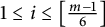 $1\leq i\leq \left [\frac {m-1}{6}\right ]$
,
 $$ \begin{align*} &B^i_1=2^{\frac{3}{2}}3^{\frac{1}{3}}A_0b^i_{1},&C^i_0&=2\mathrm{B}\left(\frac{1}{4},\frac{3}{2}\right)\sum\limits^{m-6i+1}_{j=1}jb^i_j,\\ &B^i_2|_{B^i_1=0}=\sum\limits^{m-6i+1}_{j=2}jJ_{j-1}b^i_j,&C^i_1&=2\mathrm{B}\left(\frac{3}{4},\frac{3}{2}\right)\sum\limits^{m-6i+1}_{j=1}j\left(j^2-\frac{9}{5}j+\frac{61}{25}\right)b^i_j,\\ &B^i_3=2^{\frac{1}{2}}3^{\frac{2}{3}}A_1(3b^i_{1}+4b^i_{2}),&C^i_{11}&=2\mathrm{B}\left(\frac{3}{4},\frac{3}{2}\right)\sum\limits^{m-6i+1}_{j=1}j\left(j^2-3j+\frac{91}{25}\right)b^i_j.\nonumber \end{align*} $$
Namely, for
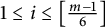 $1\leq i\leq \left [\frac {m-1}{6}\right ]$
,
 $$ \begin{align} (B^i_1,B^i_2|_{B^i_1=0},B^i_3,C^i_0,C^i_1,C^i_{11})^T=V^i(b^i_{1},b^i_{2},\ldots,b^i_{m-6i+1})^T, \end{align} $$
with the
 $6\times (m-6i+1)$
matrices
 $$ \begin{align*} V^i=\begin{pmatrix} 2^{\frac{3}{2}}3^{\frac{1}{3}}A_0 & 0 & 0 & \cdots & 0 \\ 0 & 2J_1 & 3J_2 & \cdots & n_iJ_{m-6i} \\ 2^{\frac{1}{2}}3^{\frac{5}{3}}A_1 & 2^{\frac{5}{2}}3^{\frac{2}{3}}A_1 & 0 & \cdots & 0 \\ 2\mathrm{B}\left(\frac{1}{4},\frac{3}{2}\right) & 4\mathrm{B}\left(\frac{1}{4},\frac{3}{2}\right) & 6\mathrm{B}\left(\frac{1}{4},\frac{3}{2}\right) & \cdots & 2n_i\mathrm{B}\left(\frac{1}{4},\frac{3}{2}\right)\\ \frac{82}{25}\mathrm{B}\left(\frac{3}{4},\frac{3}{2}\right) & \frac{284}{25}\mathrm{B}\left(\frac{3}{4},\frac{3}{2}\right) & \frac{906}{25}\mathrm{B}\left(\frac{3}{4},\frac{3}{2}\right) & \cdots & 2n_i(n_i^2-\frac{9}{5}n_i+\frac{61}{25})\mathrm{B}\left(\frac{3}{4},\frac{3}{2}\right)\\ \frac{82}{25}\mathrm{B}\left(\frac{3}{4},\frac{3}{2}\right) & \frac{164}{25}\mathrm{B}\left(\frac{3}{4},\frac{3}{2}\right) & \frac{546}{25}\mathrm{B}\left(\frac{3}{4},\frac{3}{2}\right) & \cdots & 2n_i(n_i^2-3n_i+\frac{91}{25})\mathrm{B}\left(\frac{3}{4},\frac{3}{2}\right) \end{pmatrix}. \end{align*} $$
According to Theorem 2, together with the definitions of
 $B_{3i+r}$
and
 $C_i$
in (39) and (40), one gets for
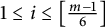 $1\leq i\leq \left [\frac {m-1}{6}\right ]$
,
 $$ \begin{align} (B_{3i+1},B_{3i+2},B_{3i+3},C_{2i},C_{2i+1},C^i_{11})^T=U^i(B^i_1,B^i_2|_{B^i_1=0},B^i_3,C^i_0,C^i_1,C^i_{11})^T, \end{align} $$
with the diagonal matrices of order 6
 $$ \begin{align*} U^i=\mathrm{ diag}\left(\frac{(-6)^i}{\prod\limits^i_{j=1}(6j+5)},\frac{1}{(i+1)!},\frac{(-6)^i}{\prod\limits^i_{j=1}(6j+7)},\frac{4^i}{\prod\limits^i_{j=1}(4j+3)},\frac{4^i}{\prod\limits^i_{j=1}(4j+5)},1\right). \end{align*} $$
Substituting (46) and (47) into (48) gives for
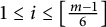 $1\leq i\leq \left [\frac {m-1}{6}\right ]$
,
 $$ \begin{align} (B_{3i+1},B_{3i+2},B_{3i+3},C_{2i},C_{2i+1},C^i_{11})^T=U^iV^i\prod\limits^{i}_{j=1}A^i_j(b_{6i},b_{6i+1},\ldots,b_{m})^T. \end{align} $$
Set
 $m-1=6n+r$
with
 $r\leq 6$
and n nonnegative integers. According to (45) and (49), one gets by means of a Python program that all Jacobian matrices
 $\frac {\partial G}{\partial (b_0,b_1,\ldots ,b_m)}$
are of full rank with
 $m\leq 300$
, where
-
• for
$1\leq r\leq 3$
,
$G=(B_0,B_1,\ldots ,B_{3n+r-1},C^0_{11},C^1_{11},\ldots ,C^{n-1}_{11},C_0,C_1,\ldots ,C_{2n-1},b)$
with
$b\in \{B_{3n+r},C_{2n}\}$
; -
• for
$4\leq r\leq 6$
,
$G=(B_0,B_1,\ldots ,B_{3n+2},C^0_{11},C^1_{11},\ldots ,C^{n-1}_{11},C_0,C_1,\ldots ,C_{2n},b)$
with
$b\in \{B_{3n+3},C_{2n+1}\}$
.






In light of Theorem 8 or Corollary 1, the Liénard differential system (43) can have
-
•
$7n+2r-1$
limit cycles for
$1\leq r\leq 3$
, obtained by taking
$r_1=r$
and
$r_2=0$
in Theorem 8; -
•
$7n+6$
limit cycles for
$4\leq r\leq 6$
, obtained by taking
$r_1=3$
and
$r_2=1$
in Theorem 8.


The proof is completed.
4.2 Proof of Theorem 6
Consider the near-Hamiltonian system of the form:
 $$ \begin{align} \dot x=y+\varepsilon P_0(x,y),\qquad \dot y=-x^3(1-x-x^2)+\varepsilon Q_0(x,y). \end{align} $$
with the perturbed polynomials
 $P_0(x,y)$
and
 $Q_0(x,y)$
of degree m. The corresponding Hamiltonian function is
 $H(x,y)=\frac {1}{2}y^{2}+\frac {1}{4}x^{4}-\frac {1}{5}x^5-\frac {1}{6}x^6$
, whose associated system has a nilpotent center of order 1 at the origin.
Set
 $G^0(x,y):=\frac {\partial P_0}{\partial x}+\frac {\partial Q_0}{\partial y}=\sum \limits _{i+j=0}^{m-1}c_{ij}x^iy^j$
. It follows from Theorem 1 and (39) that
 $$ \begin{align*} C_{0}&=2\mathrm{B}\left(\frac{1}{4},\frac{3}{2}\right)c_{00},& C_{1}&=2\mathrm{B}\left(\frac{3}{4},\frac{3}{2}\right)\left(\frac{46}{25}c_{00}-\frac{3}{5}c_{10}+2c_{20}\right),\\ C^0_{11}&=2\mathrm{B}\left(\frac{3}{4},\frac{3}{2}\right)\left(\frac{46}{25}c_{00}+2c_{20}\right),& & \nonumber \end{align*} $$
which give
 $$ \begin{align} (C_0,C_1,C^0_{11})^T=R_0(c_{00},c_{10},c_{20})^T, \end{align} $$
with
 $R_0$
a
 $3\times 3$
matrix of the form
 $$ \begin{align} R_0= \begin{pmatrix} 2\mathrm{B}\left(\frac{1}{4},\frac{3}{2}\right) & 0 & 0\\ \frac{92}{25}\mathrm{B}\left(\frac{3}{4},\frac{3}{2}\right) &-\frac{6}{5}\mathrm{B}\left(\frac{3}{4},\frac{3}{2}\right) & 4\mathrm{B}\left(\frac{3}{4},\frac{3}{2}\right) \\ \frac{92}{25}\mathrm{B}\left(\frac{3}{4},\frac{3}{2}\right) & 0 & 4\mathrm{B}\left(\frac{3}{4},\frac{3}{2}\right) \end{pmatrix}. \end{align} $$
The condition
 $\overline {\Lambda }^0=\Lambda ^0$
of Theorem 3 implies
 $\frac {\partial ^l}{\partial x^l}G^0(0,0)=l!c_{l0}=0$
for
 $l=0,1,2$
. It follows from the expression of
 $G^0$
that the equality (13) with
 $i=1$
holds by ordering
 $$ \begin{align*}P_1=\frac{G^0(x,y)|_{\overline{\Lambda}^0}}{x^3(1-x-x^2)}\quad \text{and}\quad Q_1=\frac{1}{y}(G^0(x,y)-G^0(x,0)),\end{align*} $$
which implies the expressions
 $$ \begin{align*}P_1=\sum\limits^{\infty}_{i=0}a^1_{i0}x^i\quad \text{and} \quad Q_1=\sum\limits^{m-2}_{i+j=0}b^1_{ij}x^iy^j,\end{align*} $$
with
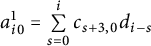 $a^1_{i0}=\sum \limits ^{i}_{s=0}c_{s+3,0}d_{i-s}$
for
 $s\leq m-4$
,
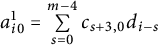 $a^1_{i0}=\sum \limits ^{m-4}_{s=0}c_{s+3,0}d_{i-s}$
for
 $s\geq m-3$
, and
 $b^1_{ij}=c_{i,j+1}$
for
 $0\leq i+j\leq m-2$
, where we have used the expansion
 $$ \begin{align} \frac{1}{1-x-x^2}=\sum\limits_{i=0}^{\infty}x^id_i, \quad d_i=\sum\limits_{j=[\frac{i+1}{2}]}^{i}\frac{j!}{(i-j)!(2j-i)!}. \end{align} $$
Set
 $$ \begin{align*}P_{l-1}:=\sum\limits^{\infty}_{i=0}a^{l-1}_{i0}x^i\quad \text{and} \quad Q_{l-1}:=\sum\limits^{n_{l-1}}_{i+j=0}b^{l-1}_{ij}x^iy^j\end{align*} $$
with
 $n_{l-1}=m-2l+2$
for
 $l\geq 2$
. Simple calculations show that
 $$ \begin{align*} G^{l-1}(x,y):=\frac{\partial P_{l-1}}{\partial x}+\frac{\partial Q_{l-1}}{\partial y}=\sum\limits_{i+j=0}^{n_{l-1}-1}c^{l-1}_{ij}x^iy^j+\sum\limits_{i=n_{l-1}}^{\infty}c^{l-1}_{i0}x^i, \end{align*} $$
where
 $$ \begin{align*} c^{l-1}_{ij}= \begin{cases} (i+1)a^{l-1}_{i+1,0}+\bar{b}^{l-1}_{i1},&j=0, \\ (j+1)b^{l-1}_{i,j+1},&j\geq1,\ 1\leq i+j\leq n_{l-1}-1, \end{cases} \end{align*} $$
with
 $\bar {b}^{l-1}_{i1}=b^{l-1}_{i1}$
for
 $0\leq i\leq n_{l-1}-1$
and
 $\bar {b}^{l-1}_{i1}=0$
for
 $i\geq n_{l-1}$
.
Recursive manipulation as above applies to the condition
 $\overline {\Lambda }^l$
and the equality (13), one gets
 $$ \begin{align*}P_l=\sum\limits^{\infty}_{i=0}a^l_{i0}x^i\quad \text{and} \quad Q_l=\sum\limits^{n_l}_{i+j=0}b^l_{ij}x^iy^j,\end{align*} $$
where
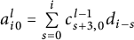 $a^l_{i0}=\sum \limits ^{i}_{s=0}c^{l-1}_{s+3,0}d_{i-s}$
with
 $d_{i}$
given in (53) for all i’s and
 $b^l_{ij}=(j+2)b^{l-1}_{i,j+2}$
for
 $0\leq i+j\leq n_l$
. Further calculations via induction yield
 $$ \begin{align} (c^1_{00},c^1_{10},c^1_{20})^T= \begin{cases} (c_{02},c_{12},c_{22})^T, & m=3,\\ a_1(c_{30},c_{40},\ldots,c_{m-1,0})^T+(c_{02},c_{12},c_{22})^T, & 4\leq m\leq6,\\ A_1(c_{30},c_{40},c_{50},c_{60})^T+(c_{02},c_{12},c_{22})^T, & m\geq7, \end{cases} \end{align} $$
and for
 $l=2,3,\dots ,\left [\frac {2[\frac {m}{2}]-2}{3}\right ]+\left [\frac {m+1}{2}\right ]-1$
,
 $$ \begin{align} (c^l_{00},c^l_{10},c^l_{20})^T=&\sum\limits^{l-1}_{i=1}(2i-1)!!\prod\limits^{l-i}_{j=0}A_j(c_{3,2i},c_{4,2i},\ldots,c_{4(l-i)+2,2i})^T\\ &\quad+(2i-1)!!(c_{0,2l},c_{1,2l},c_{2,2l})^T\nonumber\\ &\qquad+\begin{cases} \prod\limits^{l}_{j=0} A_j(c_{30},c_{40},\ldots,c_{4l+2,0})^T, & 4l\leq m-3,\\ \prod\limits^{l-1}_{j=0} A_ja_l(c_{30},c_{40},\ldots,c_{m-1,0})^T, & 4l\geq m-2, \end{cases}\nonumber \end{align} $$
where
 $A_0$
is the identity matrix of order 3,
 $A_1$
is the
 $3\times 4$
matrix
 $$ \begin{align*} &A_1= \begin{pmatrix} d_1 & d_0 & 0& 0\\ 2d_2 & 2d_1 & 2d_0& 0 \\ 3d_3& 3d_2 & 3d_1 & 3d_0& \end{pmatrix}, \end{align*} $$
 $A_j$
’s are the
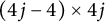 $(4j-4)\times 4j$
matrices
 $$ \begin{align*} &A_j= \begin{pmatrix} 4d_4 & 4d_3 & 4d_2&\cdots& 0\\ 5d_5 & 5d_4 & 5d_3 & \cdots& 0\\ \vdots & \vdots& \vdots & \ddots & \vdots \\ (4j-1)d_{4j-1}& (4j-1)d_{4j-2} & (4j-1)d_{4j-3} & \cdots& (4j-1)d_0 \end{pmatrix} \end{align*} $$
for
 $2\leq j\leq l$
, and
 $a_l$
’s are the
 $(4l-4)\times (m-3)$
matrices
 $$ \begin{align*} &a_l= \begin{pmatrix} 4d_4 & 4d_3 & 4d_2&\cdots& 0\\ \vdots & \vdots& \vdots & \ddots & \vdots \\ (m-4)d_{m-4} & (m-4)d_{m-5} & (m-4)d_{m-6} & \cdots& (m-4)d_0\\ (m-3)d_{m-3} & (m-3)d_{m-4} & (m-3)d_{m-5} & \cdots& (m-3)d_1\\ \vdots & \vdots& \vdots & \ddots & \vdots \\ (4l-1)d_{4l-1}& (4l-1)d_{4l-2} & (4l-1)d_{4l-3} & \cdots& (4l-1)d_{4l-m+3} \end{pmatrix} \end{align*} $$
for
 $l\geq 2$
, and
 $a_1=(a^1_{ij})$
is the
 $3\times (m-3)$
matrix with
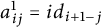 $a^1_{ij}=id_{i+1-j}$
for
 $i+1\geq j$
, and
 $a^1_{ij}=0$
for
 $i+1< j$
. We remark that for compactness to notations, we have introduced
 $c_{ij}=0$
for
 $i+j\geq m$
in (54) and (55).
By Theorem 1 and (12), one has for
 $l=1,2,\dots ,\left [\frac {2[\frac {m}{2}]-2}{3}\right ]+\left [\frac {m+1}{2}\right ]-1$
,
 $$ \begin{align} (C^l_0,C^l_1,C^l_{11})^T=R_0(c^l_{00},c^l_{10},c^l_{20})^T \end{align} $$
with the matrix
 $R_0$
given in (52). According to Theorem 3 and the definitions of
 $C_{2i+j}$
’s in (42), one further has for
 $1\leq l\leq \left [\frac {2[\frac {m}{2}]-2}{3}\right ]+\left [\frac {m+1}{2}\right ]-1$
,
 $$ \begin{align} (C_{2l},C_{2l+1},C^l_{11})^T=U_l(C^l_0,C^l_1,C^l_{11})^T \end{align} $$
with the diagonal matrices of order 3
 $$ \begin{align*} U_l=\mathrm{diag}\left(\frac{4^i}{\prod\limits^i_{j=1}(4j+3)},\frac{4^i}{\prod\limits^i_{j=1}(4j+5)},1\right). \end{align*} $$
Substituting (54) and (55) into (56) and (57) gives
 $$ \begin{align} (C_{2},C_{3},C^1_{11})^T = U_1R_0(c_{02},0,0)^T \end{align} $$
for
 $m=3$
, and
 $$ \begin{align}(C_{2l},C_{2l+1},C^l_{11})^T=&\sum\limits^{l-1}_{i=1}(2i-1)!!U_lR_0\prod\limits^{l-i}_{j=0}A_j(c_{3,2i},c_{4,2i},\ldots,c_{4(l-i)+2,2i})^T\nonumber\\ &\quad+(2i-1)!!U_lR_0(c_{0,2l},c_{1,2l},c_{2,2l})^T\nonumber\\ &\qquad+\begin{cases} U_lR_0\prod\limits^{l}_{j=0} A_j(c_{30},c_{40},\ldots,c_{4l+2,0})^T, & 4l\leq m-3,\\ U_lR_0\prod\limits^{l-1}_{j=0} A_ja_l(c_{30},c_{40},\ldots,c_{m-1,0})^T, & 4l\geq m-2 \end{cases} \end{align} $$
for
 $m\geq 4$
and
 $1\leq l\leq \left [\frac {2[\frac {m}{2}]-2}{3}\right ]+\left [\frac {m+1}{2}\right ]-1$
, where the summation
 $\sum \limits ^{l-1}_{i=1}$
is null if
 $l=1$
, and
 $c_{ij}=0$
if
 $i+j\geq m$
.
One can check easily from formulas (51), (58), and (59) that
 $C_l$
’s and
 $C^l_{11}$
’s depend merely on the parameters
 $c_{i,2j}$
with
 $i+2j\leq m-1$
. Set
 $E_m:=\{c_{i,2j}:i+2j\leq m-1\}$
. Observe that
 $E_m$
contains
 $[\frac {m+1}{2}][\frac {m+2}{2}]$
elements. Set
 $3[\frac {m+1}{2}]+2[\frac {m}{2}]-4 =3n+r$
with
 $r\leq 2$
and n nonnegative integers.
For
 $m=1,2$
, it follows from (51) that the Jacobian matrices
 $\frac {\partial (C_0,\ldots ,C_m)}{\partial E_m}$
are of full rank.
For
 $m\geq 3$
, it follows from (51) and (57), together with a Python program that all Jacobian matrices
 $\frac {\partial G}{\partial E_m}$
are of full rank with
 $m\leq 22$
, where
 $G=(C_0,C_1,\ldots ,C_{2n+r-1},C^0_{11},C^1_{11},\ldots ,C^{n-1}_{11})$
. These together with Theorem 10 or Corollary 3 prove that the near-Hamiltonian system (50) can have
 $2n+r-1$
limit cycles.
This proves the theorem.
We remark that Theorems 5 and 6 both have limitations on the degree m of the perturbed polynomials. These have been used in calculations of the ranks of the Jacobian matrices, supported by two Python programs available in our GitHub repository: https://github.com/grass2sturdy/Rank. Theoretically, these calculations work by Python programs for any m. But in practice, it depends on memory of computers.
5 Conclusions
A lot of papers studied the coefficients in the expansion of the first-order Melnikov function near a homoclinic loop with a nilpotent singularity in a near-Hamiltonian system. Based on the existing results, Yang et al. [Reference Yang, Yu and Han63] and Wei and Zhang [Reference Wei and Zhang52] presented the coefficients of the terms with degree less than 2 in the case of a nilpotent singularity of arbitrary order. Moreover, Yang and Han [Reference Yang and Han62] pushed further the relation between the coefficients of the terms with the same order in the expansions inside or outside a cuspidal loop. The characteristics of the coefficients, of the terms with degree greater than or equal to 2, were developed further and exhibited in [Reference Wei and Zhang52, Reference Yang, Yu and Han64] provided that the center is elementary. If the center of the unperturbed Hamiltonian system is nilpotent, as well as the homoclinic loop approaches also to a nilpotent singularity, the problem remains open. This article tackles this problem.
The work in this article presents the accurate expressions of the first
 $\frac {k}{2}$
coefficients in the asymptotic expansion of the first-order Melnikov function near a nilpotent center of order k, and characterizes its higher-order coefficients, which are given in Theorems 1 and 3, respectively. Based on these results, our primary motivation is to depict the features of the higher-order coefficients in the first-order Melnikov function near a homoclinic loop to a nilpotent singularity of arbitrary order, in virtual of the nilpotent center of arbitrary order inside the loop that the unperturbed Hamiltonian system has. The related results are given in Theorem 2. On account of these established results, we further investigate the limit cycle bifurcations near either a nilpotent center or a homoclinic loop to a nilpotent singularity.
At last, we apply our results to two concrete systems, an
 $(m+1)$
th-order Liénard differential system and an mth-order near-Hamiltonian differential system with a hyperelliptic Hamiltonian, for achieving more number of limit cycles, which are bifurcated from periodic orbits either near a nilpotent center or near a homoclinic loop to a nilpotent singularity.