

Motivation
Our planet has experienced a rapid change of the global climate within the last 100 years, and this has had a pronounced impact on the Arctic and Antarctic environment. The rise of sea level due to global warming is considered one of the main natural threats for human society. The melting of polar ice masses causes the main portion of this sea level rise. Taken together, the present global cryosphere (glaciers and ice sheets) contains sufficient water to raise sea level by almost 70m. Thus, a small fraction of change in their volume would have a significant effect on sea level (Rack and others Reference Rack, Nixdorf, Miller and Runge2004). To evaluate the contribution of polar ice caps to the observed changes, regular observation of large polar areas is necessary. Because of the remoteness and the harsh climatic conditions of polar regions satellite based SAR sensors are best suited for their observation.
The capability of SAR interferometry (InSAR) in terms of deformation monitoring and topographic mapping has been proved by various case studies during the last decades. The first InSAR based analysis of the flow of an ice stream was published in 1993 by Goldstein and others (Reference Goldstein, Engelhardt, Kamb and Frolich1993). In recent years, the focus of investigation has changed towards a detailed analysis of potential error sources, such as temporal and geometrical decorrelation, atmospheric path delay, surface penetration, and orbit uncertainties. The analysis of stable targets, so called permanent scatterers, identified from a number of interferograms enables us to minimise the effect of temporal and geometrical decorrelation and to mitigate large parts of the atmospheric path delay. However, due to the lack of stable targets, this method cannot be applied for the analysis of glaciers and ice sheets, which is a well-known application of InSAR. Thus, the evaluation of possible error sources is still a challenging problem in glacier monitoring.
This paper presents an estimation method to determine the topography and motion of polar ice masses from SAR interferograms. The approach is focused on a systematic modelling of all processing steps and their particular stochastic properties. The functional and stochastic description of all influences on the interferometric phase signal serves as the basis for a detailed analysis of accuracy, robustness and gross errors of the estimated results. Special emphasis is put on the investigation of influences from topography and motion, as well as the effects of orbit errors, atmospheric path delays, and the penetration depth of the signal into the surface.
Method
The goal of this work is to use the information inherent in a set of temporarily and spatially diverse SAR interferograms for an accurate and robust estimation of parameters of interest. For this, a framework is necessary that allows combining diverse data sets in a systematic and consistent manner. The theory of least-squares adjustment, which is widely used in engineering applications, is perfectly suited for this purpose.
Adjustment model
The aim of all adjustment methods is to map a number of n uncertain observations b on a number of u<n unknown parameters x. This step requires the formulation of functional relations between observations and unknowns. The functional model of a least-squares adjustment based on erroneous observations is defined by:

with  being the estimated values of residuals and the estimated unknowns . If accuracy measures for the observations are available, weighting of the observations may be performed. Observations with high accuracy will receive high weights and will therefore have strong influence on the estimated parameters and vice versa. The a priori information about the accuracy of the observations is called stochastic model and is arranged in the so called covariance matrix Kbb.
Following the Gauss-Markov theory, the optimal solution of an over-determined equation system such as that shown in equation (1) is derived by minimising the objective function:

with . Solving this minimisation problem yields the adjusted unknowns as well as their theoretical accuracies relations expressed by the matrix:

with A comprising the functional relations and containing approximate values for the unknowns (Mikhail Reference Mikhail1976).
Observations and unknowns
Based on observations derived from SAR data the unknown topography and motion of polar glaciers are estimated. As SAR is only sensitive to the surface motion component lying in the line of sight of the sensor this component of a three dimensional surface motion can be determined only within the adjustment. Thus, v is defined as a change of the line of sight position of a surface element per time and always corresponds only to the line of sight component of surface motion.
SAR SLCs of the ERS C-band SAR serve as the primary data source. From this data set, SAR interferograms are formed. Unfortunately, the temporal baseline of the interferograms cannot be arbitrarily chosen. is above all limited by temporal decorrelation. Especially in snow-covered polar regions changing wind conditions, temperature variation, and precipitation result in a strong decrease of correlation over time. To guarantee interferograms with sufficient quality, interferograms originating from the ERS tandem mission comprising a temporal baseline of only a single day should be preferred. Before implementing the data into the adjustment, two preparatory steps are necessary. The first of these is that the ambiguous interferometric phase values are unwrapped based on a minimum cost flow approach. For a detailed description of the unwrapping algorithm used reference should be made to Costantini (Reference Costantini1998). The second preparatory step is that a reference phase screen is subtracted from the interferograms beforehand using ERS D-PAF precise orbit information.
Functional model
As described above, the functional model comprises the deterministic relations between observations and unknowns. For solving the proposed problem, the functional model consists of three different sub-models. The formulation of the sub-models and their particular characteristics are derived in the following.
Interferometric model
Although the phase ɸ of an interferogram acquired over glaciated terrain is influenced by many parameters, ɸ is dominated by influences from surface topography h, coherent motion v in line-of-sight of the sensor, the difference of the slant-atmospheric delay Δsd between the two acquisitions, and the penetration depth d of the RADAR signal into the glacier surface. The unwrapped interferometric phase at position (i, j) of an interferogram may be written as:
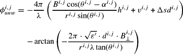
The notation used in the equation is in accordance with Hanssen (Reference Hanssen2001). The four different parts of equation (4) show the mathematical description of the above mentioned influences onto the interferometric phase. The geometric reference phase is already corrected in this representation. According to equation (4) each interferometric phase observation induces four unknown parameters (h, ν, Δsd, d) per pixel. Thus, the inversion of the model is a highly underdetermined problem. A solution can be found if i) additional observations are incorporated on a pixel by pixel basis, or if ii) prior information is integrated into the equation system. The second strategy might be employed if one or more parameters of the equation system are known (for example external DEMs, or knowledge about surface deformation). Such information is mostly not available in the arctic environment. Thus, a solution has to be found by a combination of a series of interferograms in consideration of additional assumptions about the temporal evolution of some parameters.
Temporal model
In order to guarantee a successful separation of the phase components in equation (4), functional relations describing the connection between unknowns in different data sets have to be established. Such models are only found for deterministic processes, that is signals that do not arise from a stochastic process. In principle, this only holds for the evolution of topography and surface displacement. As topographical changes are usually slow, and because of the limited sensitivity of the interferometric phase to such variations, a time independent description of surface topography h has been chosen. Introducing this model reduces the number of topography-related unknowns from N · i · j unknowns to i · j unknowns.
As described in Fatland and Lingle (Reference Fatland and Lingle1998) and Frolich and Doake (Reference Frolich and Doake1998) the assumption of constant glacier flow is doubtful and only holds for glaciers that are frozen to the bedrock (so called cold glaciers) and therefore show a purely laminar flow. Temperate glaciers however usually show significant temporal changes of their flow on a variety of time scales. Here the percentage change of velocity usually increases with decreasing length of the observation interval. Thus, if polar glaciers are observed by SAR interferometry, which is characterised by short observation intervals of a single day or only a few days, short term flow variations cannot be neglected. To allow for a time-variant flow v(t) a mathematical model is employed. We refrain from using physical flow models, because of their high complexity, significant non-linearity, and limited quality. As least-squares adjustments are better suited for solving linear problems, linear models for describing the glacier flow are favoured. Considering the usually uneven distribution of the data sets over time a piecewise Lagrange polynomial is selected. The maximum polynomial order equals , where uv is the number of parameters not related to surface motion. The term −1 warrants a redundant equation system. Thus, the surface motion v(t) is modelled by
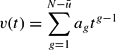
Spatial model
The unknown parameters are not solved in each pixel but rather in the nodes of a regular spatial grid. This step is allowed if the sampling rate of the digital data sets is higher than necessary for the representation of their information content. The restriction of calculating the desired parameters only in a coarser grid entails several advantages. On one hand, it reduces processing time, while on the other hand, it increases redundancy and, by this, the ability of the adjustment to detect gross errors in the observations. The mesh size has to be chosen properly to avoid under-sampling. Bilinear planes have been selected for approximating the spatial correlation of topography and motion. The functional relation between an observed phase value in an arbitrary position ɸi,j and an unknown value in a node of the corresponding bilinear raster ɸk,l is given by:

where .
Although using the proposed models allows reducing the number of unknowns, the equation system is still underdetermined. This is due to the unmodelled atmospheric artefacts and the unknown penetration depth. In Hanssen (Reference Hanssen2001) a stochastic model for approximating the influence of the atmosphere on SAR interferograms is proposed, which is based on the spatial correlation of the atmospheric signal. As the atmosphere in the arctic area cannot hold much water vapour and is usually characterised by a stable stratification, and as the region of interest in the presented example is of small extent, atmospheric effects are neglected in this study. The penetration depth of C-band SAR signals into firn and ice was studied in detail by Hoen (Reference Hoen2001). Maximal penetration depth into dry snow is shown to be up to 30m. In this paper penetration depth is considered constant in time. Influences by constant penetration depth are considered as part of the topography component.
Stochastic model
Weighting of observations is done based on the coherency of the interferometric phase values. From the coherency the probability density function (PDF) of the interferometric phase for each resolution cell is derived using the theory described by Bamler and Hartl (Reference Bamler and Hartl1998) and by Lee and others (Reference Lee, Hoppel and Mango1994). Finally, the standard deviations σφ of the observed phase values are derived from the PDF function via:
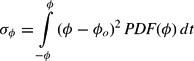
where ɸ0 is the expectation value of the interferometric phase. From the standard deviations, the weight matrix is deduced assuming uncorrelated observations. The stochastic model derived in this way implicitly accounts for noise introduced by temporal, thermal and geometric decorrelation as well as errors originating from imperfect interpolation and co-registration procedures.
Additional variance and covariance values are usually introduced by orbit errors and atmospheric effects. These additional error sources are neglected in this study for the following two reasons: i) Orbit errors have been significantly reduced using precise orbit information in combination with control points. ii) Atmospheric effects showed to be small in polar regions as their cold atmosphere appears to be very stable and cannot hold much water vapour. The impact of neglecting atmospheric effects on the estimated unknowns is analysed in more detail in the following section. This analysis takes in account the peculiarities of the polar atmosphere.
Analysis of the approach
Accuracy analysis
The diagonal of (see equation (3)), which contains information about the variances of the adjusted parameters, is used to derive theoretical standard deviations of topography and surface motion. For analysing the accuracy of the approach, simulated data sets have been generated based on existing DEM and velocity maps. The coherency estimates of each simulated interferogram account for the local surface slope. The simulated data sets are implemented into the adjustment and the resulting matrices are analysed.
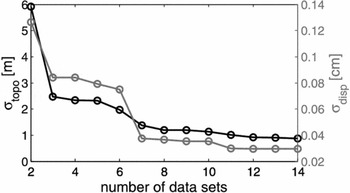
In a first step, the dependency of σtopo and σdisp on the number of independent data sets is investigated by changing the number of input interferograms. The results of this analysis are presented in Fig. 1. The improvement attained by adding more interferograms to the adjustment is clearly visible. For a high number of data sets, both topography and glacier flow can be estimated with high accuracy.
Theoretical standard deviations σtopo σ topo (black) and σdisp σ disp (grey) dependent on the number of data sets.

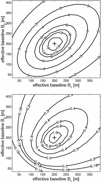
Fig. 2 shows how the standard deviations of the estimated topography and displacement parameters depend on the observation geometry, which is mainly a function of the interferometric baseline B. The presented results are calculated based on three simulated interferograms. In 256 simulation runs, the baselines of the interferograms 1 and 2 are varied from 0m to 400m each. The baseline of the third interferogram is fixed at 200m. In general, the standard deviations of both topography and motion show distinct dependency on the baseline ratio of the involved interferograms.
a) Mean standard deviation of topography (m) and b) mean standard deviation of displacement parameters (mm/day) as a function of baseline constellation. The effective baseline length of B3 is set to 200m.

Baselines of similar length result in a weak configuration of the adjustment model and finally, in increased values for σtopo, and σdisp. In case of identical baselines, the adjustment becomes singular (this case is indicated by the cross in Fig. 2). If the baselines of the three interferograms are well distributed, the topographic height may be estimated with an accuracy of σtopo ≈ 3m and the surface motion with a standard deviation of σdisp ≈ 1 – 2mm/day. A more detailed inspection of Fig. 2 shows, however, that topography and displacement uncertainties are not minimised by the same measurement setup. σtopo is decreasing for well distributed long baselines; optimal accuracies of surface motion arise if all baselines are short.
Sensitivity to model errors
The interferometric model presented in equation (4) has been simplified by neglecting the influences of atmospheric effects and penetration depth. If these non-modelled influences are significant, model errors are introduced resulting in a systematic falsification of the estimated unknowns.
Atmospheric effects
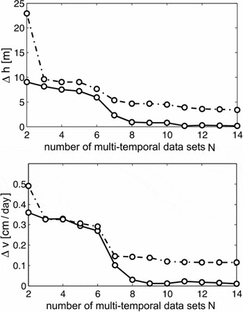
As interferograms infer purely relative measurements, the theoretical expectation value of atmospheric effects will be zero for an arbitrary pixel. However, the variance of the signal might be significant depending on the respective weather conditions. If sufficient observations are combined, the empirical expectation value, which is estimated from the data, approaches the theoretical value. Thus, for large number of observations, atmospheric effects will cancel out more and more. The effect of non-modelled atmospheric influences on the estimated unknowns has been calculated for varying observation configurations. Atmospheric phase screens have been simulated based on a method presented by Hanssen (Reference Hanssen2001) considering the effect of the polar atmosphere on the interferometric phase as described in Gray and others (Reference Gray, Mattar, Geudtner and Vachon1997). Fig. 3 shows the effect of the polar atmosphere on the unknown topography h and motion v as a function of the number of multi-temporal data sets. The solid lines in Fig. 3 show the systematic error of the estimated topography (Fig. 3a)) and motion (Fig. 3b)). For a low number of data sets, topography may be falsified up to Δh = 10 m, the estimated motion up to Δν = 0.4cm/day. With increasing number of data sets Δh and Δν approach zero as expected. For investigating whether Δh and/or Δν differ significantly from zero, a significance test is performed. The dashed lines in Fig. 3 represent the upper acceptance limit for the null hypothesis. Values above the dashed line are significant. Values below are insignificant. Fig. 3 shows that in Arctic regions systematic errors of the adjusted unknowns due to atmospheric effects are insignificant for all tested configurations.
a) Effect of non-modelled atmospheric effects on the estimated unknowns topography (a)) and motion (b)) for polar regions.

Penetration depth
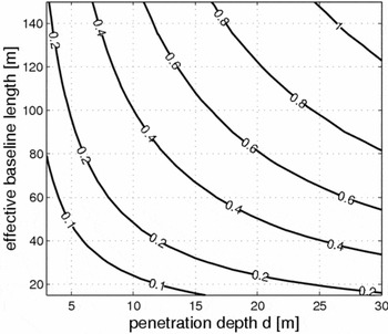
The penetration depth d of a radar signal into the glacier surface depends mainly on the wavelength of the transmitted signal and the physical properties of the upper surface layers. As presented in Hoen (Reference Hoen2001), C-band signals penetrate up to 27±5m into cold firn. The impact φ pd on the interferometric phase increases with the interferometric baseline. Fig. 4 shows the dependence of φ pd on d and B for C-band SARs.
Effect of penetration depth on the interferometric phase [rad].

A temporarily constant penetration d results in a systematic under-estimation of the glacier topography. This topographic height error is given by
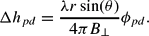
Considering a typical baseline of B = 100m and the sensor parameters of the ERS satellite the true glacier surface might be under-estimated by up to 100m.
Improperly chosen temporal model
An improperly chosen temporal model may also introduce systematic errors. In common d-InSAR approaches the flow of a glacier is usually considered to be constant in amplitude and flow direction throughout the whole observation period. An analysis based on simulated data sets should answer the question about the estimation errors occurring due to violations to this simplified flow model. The topography related phase is simulated based on an available DEM of a test glacier (Sonklar glacier, Ostrov Gallya [Hall Island], Zemlya Frantsa-Iosifa [Franz Josef Land]). The motion part of the phase is derived from the real glacier flow field and multiplied by a linear time dependent factor (see equation (5)) yielding a linearly accelerating flow field. Tests with varying acceleration rates showed that the resulting systematic errors are significant for all test scenarios and for both topography and motion. Increasing the number of data sets permits a significant reduction in the topography error Δh, but motion errors appear nearly unchanged.
Validation
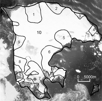
In this section the presented estimation method is validated based on multi-temporal data sets of a test area in the Russian high arctic. Ostrov Gallya is one of the largest islands of the Russian archipelago Zemlya Frantsa-Iosifa. Situated approximately at 80°10′ N and 58°05′ E, its variety of topographical and glaciological forms as well as drastic changes of its environment attracts the attention of glaciologists. An impression of Ostrov Gallya is given in Fig. 5.
KATE-200 image of Ostrov Gallya [Hall Island], Zemlya Frantsa-Iosifa [Franz Josef Land] superimposed by coarse information about its coastline (bold) and glacier margins (thin) taken from (Vinogradov and Psaryova Reference Vinogradov and Psaryova1965).

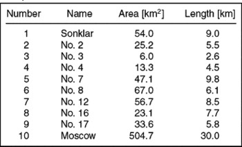
Approximately 90% of the island is covered by the so-called Moscow Ice Dome the ice masses of which flow into the sea along several large outlet glaciers. Ice free areas appear mainly in the north of the island and on the two headlands in the south-east (hatched areas in Fig. 5). Nearly 50% of the shoreline is dominated by the calving ice fronts of the large outlet glaciers. Some information about the most important outlet glaciers on Hall Island is included in Table 1. The numbers in the first column of Table 1 correspond to the numbering in Fig. 5.
Information about the largest outlet glacier on Ostrov Gallya according to (Vinogradov and Psaryova, Reference Vinogradov and Psaryova1965).

Data sets
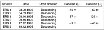
During the tandem- and ice-phase mission of the ERS1/2 satellite system several data sets were acquired over the area of interest. Six ERS SAR SLCs recorded during the ERS1/2 tandem mission were chosen for further processing. Meteorological data was consulted for the selection of suitable SAR scenes to warrant comparable atmospheric conditions for all observations. All images were acquired in 1995 and cover the period from summer to winter. The properties of the data sets are shown in Table 2. The interferometric processing of the complex SAR images has been accomplished with the Doris v3.6 software developed at the Delft Institute for Earth-Oriented Space Research of the Technical University Delft, in the Netherlands.
Properties of used SAR data.

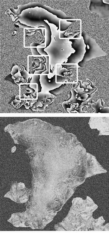
The phase and coherency image of a subset of the interferogram acquired in September 1995 that covers Ostrov Gallya, are shown in Fig. 6. For presentation purposes the phase of the interferogram in Fig. 6a was smoothed using a Goldstein-filter. Areas with large displacement related phase components are marked by white frames. The framed regions correspond to the catchment areas of the outlet glaciers Sonklar, No. 7, No. 8, No. 12 and No. 17 (see Table 1 and Fig. 5). Before inserting the data sets into the parameter estimator, some pre-processing steps are necessary. The most important step is the unwrapping of the initially ambiguous interferometric phase values. In addition the data sets are co-registered and phase ramps originating from orbit errors are removed based on control point information.
Phase image (a) and coherency image (b) of the September interferogram of Ostrov Gallya. The baseline of the interferogram is ≈50m. The phase image has been smoothed for presentation purposes.

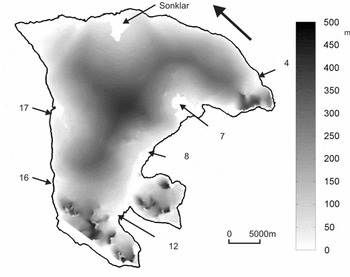
DSM of Ostrov Gallya derived from the interferometric phase. The black arrow indicates the viewing direction of the sensor. The positions of the largest outlet glaciers are indicated.

Estimation results
The pre-processed data sets form the vector of observations b in the estimation approach. Within the adjustment the unknown topography and motion parameters are estimated in the nodes of the chosen spatial model. To reduce the computational load the area of interest is separated into tiles, which are evaluated separately and re-merged afterwards. Finally, topography and motion values in all resolution cells (i; j) are interpolated from the estimated unknowns in the bilinear grid based on the mapping function of the spatial model. Thus, an area-wide DSM and velocity field is available after the process.
Digital surface model of Ostrov Gallya
Fig. 7 shows the DSM of Ostrov Gallya derived from the interferometric phase using the proposed method. The topographic height values shown in Fig. 7 are referenced to the WGS84 ellipsoid and vary within 0m–500m. The topography gradient is small in the glaciated terrain. Rough terrain only appears in the mountainous regions in the southwestern and eastern parts of the island.
Standard deviations for the height values are extracted from the covariance matrix , which is estimated within the adjustment. is defined by
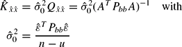
Equation (9) shows that the standard deviations of the adjusted unknowns are a function of the a priori defined functional and stochastic model as well as of the variance factor , which is estimated within the adjustment. may be interpreted as a link between the implemented models and the real data. Its values indicate to what extent the chosen functional and stochastic model fit the measured data sets. The a priori value of is set to unity before the adjustment is run. Significant deviations of the estimated a posteriori value from (1) indicate errors in the models or gross errors in the data. A separate a posteriori variance factor is estimated for each of the tiles.
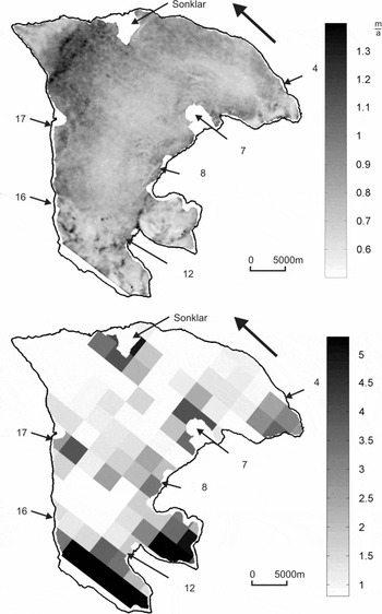
The standard deviations of the adjusted topographic heights are presented in Fig. 8, split into the theoretical standard deviations (diagonal elements of matrix ) and the estimated variance factors for each of the tiles. The black arrow indicates the viewing direction of the sensor during acquisition. The parted representation entails several advantages. The theoretical standard deviations offer an insight into the properties of the adjustment's configuration (see Fig. 8a). They illustrate the spatial distribution of the achievable height accuracy assuming a precise functional and stochastic model. Fig. 8a shows that the design of the adjustment allows estimating topography with high accuracy all over the island. The estimated variance factors presented in Fig. 8b indicate in which parts of the island the measured data sets are sufficiently described by the implemented models. Low values for appearing in large parts of the Moscow Ice Dome depict good agreement between model and data. Large values, which are visible in mountainous areas and in the catchments of the glaciers Sonklar No. 7 and No. 8, indicate model errors. In the mountainous areas these errors are due to phase unwrapping problems. In the glacier catchments this errors are caused by an insufficient flow model.
a) Theoretical standard deviations of the estimated DSM [m]. b) Adjusted variance factors for Hall Island. One variance factor is estimated for each of the tile.

The real standard deviations of the estimated topographic heights (diagonal of ) reach to in the glaciated terrain and lie between and in mountainous areas. In glaciated regions the standard deviations are in the range of the theoretical values estimated earlier on the basis of theoretical data. Due to model errors the standard deviations in mountainous terrain are larger than the simulated ones.
Velocity field of Moscow Ice Dome
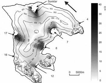
To the best of the author's knowledge no detailed velocity map of the glaciers on Ostrov Gallya has been published. Thus, the results of this study provide a new insight into the rheology and the physical properties of the ice masses on Ostrov Gallya. The estimates for the line-of-sight velocity components of the Moscow Ice Dome are presented in Fig. 9 in m/a.
Velocity field of Ostrov Gallya derived from the interferometric phase. The black arrow indicates the viewing direction of the sensor. The positions of the largest outlet glaciers are indicated.

As expected, it is mainly the glaciers Sonklar, No. 7, No. 8, No. 12, No. 16 and No. 17 that are reflected in the interferometric phase. This is because the flow direction of these glaciers is approximately directed in the sensor's line-of-sight. Besides those glaciers, the motion of glacier No. 4 is visible. The transition from stable to moving ice is smooth for all glaciers. The absolute value of the line-of-sight velocities of the Moscow Ice Dome varies from 0 m/a in ice-free areas and in the centre of the island, to 43 m/a near the front of some of the outlet glaciers. The velocity of all glaciers increases from the centre of the island towards the glacier terminus. The tongue of the largest outlet glaciers suffers from strong temporal decorrelation. Thus, the processing of glacier velocities in the frontal parts of some glaciers was not possible.
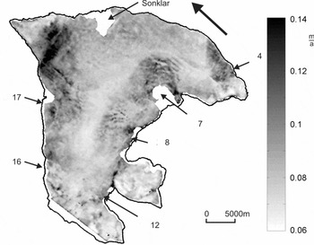
The theoretical standard deviation of the line-of-sight velocity field is shown in Fig. 10. The a posteriori variance factors for the velocity field are identical to the respective values for the estimated topography. Thus, refer to Fig. 8b to receive an impression of their spatial variation. The spatial distribution of theoretical standard deviations of the estimated velocities differs from the structure of the topography values. This is due to the fact that velocity estimates are mainly defined by interferograms with short baselines, whereas topography is especially influenced by interferograms with long baselines. In glaciated regions the real standard deviations (diagonal of ) of the velocity estimates vary between 0.1 m/a and 0.7 m/a and are in the range of the theoretical values estimated earlier in this paper. Due to model errors, the standard deviations in mountainous terrain are larger than the simulated ones.
Theoretical standard deviations of the estimated velocity field [m/a]. The respective adjusted variances factors for Ostrov Gallya can be found in Fig. 8b).

Interpretation of the residuals
During the estimation process several gross errors and model errors may occur that affect correctness and reliability of the adjusted results. These errors differ in their origin and in the structure and magnitude of their effects. They include errors during SAR data acquisition, data processing and phase unwrapping, wrongly determined stochastic properties, and insufficient functional relations. Hence, the development of a reliable estimation method that allows revealing gross errors in the data is one of the most important goals of system design.
Within the presented adjustment framework several indicators are available that allow the analysis of the robustness and reliability of the estimation setup. All of them are deduced from the following equation:

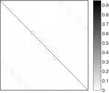
This describes how gross errors Δb in the observations and model errors are reflected in the vector of adjusted residuals . The matrix Ψ that maps Δb onto the vector of adjusted residuals is presented in Fig. 11. The structure of matrix Ψ entails some convenient properties. The diagonal elements of Ψ are close to unity, thus gross errors have a strong impact on and are therefore easily detectable. The off-diagonal elements are small. Hence, an error in observation i only affects its associated residual and a dispersion of errors does not occur.
Structure of matrix Ψ for a subset of the area of interest consisting of 10×10 pixel size.

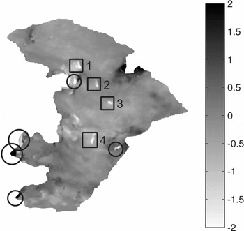
Because of these properties of the approach, the vector of residuals can be consulted for analysing gross errors in the data and the models. For the given example, an analysis of has been performed. Fig. 12 shows the phase residuals for the third interferogram acquired in December 1995. The residuals after the adjustment process are small for large areas of the island (grey coloured areas). Still there are distinct isolated regions in which the residuals are high. These regions are marked by black circles or rectangles in Fig. 12. A thorough analysis of the phase residuals together with information about the phase unwrapping process shows that the high values indicated by circles are caused by errors during the phase unwrapping procedure. The combined occurrence of high phase noise and steep slopes prevents the correct reconstruction of the absolute phase in these regions.
Adjusted residuals of the December interferogram.

A comparison of the residual maps with the interferograms proofs that the residuals in rectangle 1 (see Fig. 12) are most probably caused by an opening crack in the glacier surface. The surface below the crack moved between 4 and 5 September 1995 about 20cm relative to its surrounding and caused an un-modelled non-linear displacement component. The anomalies marked by rectangles 2–4 are similar in shape and geographic location. All of them are located along the crest of the ice cap. After an inspection of all available information the most probable explanation for the phase residuals is a local lowering of the glacier surface by about 2.5cm to 3cm in September 1995.
Summary
The approach presented in this paper allows for an improved separation of topography and displacement-related contributions to the interferometric phase by combining multi-temporal SAR interferograms in a least-squares adjustment. The interpretability of the adjusted parameters is significantly increased by a systematic model-based quantification of all influences on the interferometric signal. The capability of the method to improve the accuracy of topography and displacement estimates, as well as the possibility of revealing gross errors in the observations has been demonstrated. A brief analysis of possible error sources has been presented. A validation using real data from an island in the Russian Arctic confirms the approach.
The presented method requires phase unwrapping in the given formulation. However, if a sufficient amount of data is available, phase unwrapping can be included in both the functional and stochastic model. The impact of the integration of phase unwrapping on the performance of the approach has yet to be studied.