1. Introduction
Internal waves play an important role in the Earth's climate system because these waves contribute to the global ocean transport and dissipation, which are vital to maintaining oceanic flows such as the meridional overturning circulation (Wunsch & Ferrari Reference Wunsch and Ferrari2004). In addition, these waves, especially large-amplitude internal solitary waves, usually induce turbulence at wave breaking and strong shear currents in areas they pass through and thus impact the marine ecosystem, offshore engineering and military applications like submarine navigation and detection. Internal waves have been observed in numerous sites around the world's coastal ocean. It is generally accepted that one of the significant generation mechanisms of these waves arises from barotropic tidal or other currents flowing over topography in the stratified ocean. From the place of generation, internal waves can propagate several hundred kilometres towards the continental shelf. During these long-distance travels, various factors, including (among others) variable topography, background currents and the Earth's rotation, can modulate the waveform leading to distinct wave patterns.
Theoretical analysis is one of the most important means of investigating internal solitary waves. However, most theoretical studies are based on horizontally one-dimensional models, such as the celebrated Korteweg–de Vries (KdV) equation and its numerous variants, the Benjamin–Ono (BO) equation, and the Miyata–Choi–Camassa (MCC) equation (the interested readers are referred to Helfrich & Melville (Reference Helfrich and Melville2006), Choi & Camassa (Reference Choi and Camassa1996, Reference Choi and Camassa1999), Camassa et al. (Reference Camassa, Choi, Michallet, Rusås and Sveen2006) for more details). These models are reasonable, at least when the attention is focussed on a section plane that is generally far from the boundary or insensitive to the input from the boundary. Nevertheless, this is not appropriate for some general cases, for instance, when the interested region is too large to ignore three-dimensional effects.
For the study of horizontally two-dimensional internal waves, the Kadomtsev– Petviashvili (KP) equation (Kadomtsev & Petviashvili Reference Kadomtsev and Petviashvili1970), which is a generalisation of the KdV equation featuring uni-directional wave propagation with slight inhomogeneity in the transverse direction, has mostly been implemented (see, for example, Grimshaw & Melville Reference Grimshaw and Melville1989; Pierini Reference Pierini1989; Chen & Philip Reference Chen and Philip1995; Yuan et al. Reference Yuan, Grimshaw, Johnson and Wang2018a,Reference Yuan, Grimshaw, Johnson and Chenb). In addition, the KP equation, generally in a succinct form, has been extensively investigated from a rigorous mathematical point of view (see Biondini & Pelinovsky (Reference Biondini and Pelinovsky2008) and references therein), which facilitates the understanding of the dynamics of weakly nonlinear free-surface/internal waves in the long-wave approximation. While anisotropic uni-directional models have been successful in many aspects of the water wave problems, there are still some limitations. They cannot correctly describe the two-way propagation of water waves, such as wave reflection/transmission at seamounts and head-on collisions of solitary waves. Additionally, it is not suitable to use an anisotropic model to study wave phenomena whose transverse variations are similar to those in the primary direction of propagation. To overcome these shortcomings as well as afford a significant simplification over the primitive equations, Yuan, Wang & Chen (Reference Yuan, Wang and Chen2020) recently modified the classic Benney–Luke equation that is both isotropic and bi-directional (Benney & Luke Reference Benney and Luke1964) to make it applicable to internal waves. In their paper, however, the derived equation can only model the wave generation process and not the effects of topography on the propagation of internal waves, which is the primary concern of the present paper.
On the ocean surface, a striking feature of two-space-dimensional nonlinear waves is the oblique interactions of line solitons in the shallow water regime that form X, Y and more complex wave patterns, as shown, for instance, in photos taken by Ablowitz & Baldwin (Reference Ablowitz and Baldwin2012) and in laboratory experiments conducted by Li, Yeh & Kodama (Reference Li, Yeh and Kodama2011) and Yeh & Li (Reference Yeh and Li2014). These distinctive wave patterns are persistent in nature and can be qualitatively understood by solving the KP equation for interacting line solitons (Ablowitz & Baldwin Reference Ablowitz and Baldwin2012). By applying an inverse scattering method, Zakharov & Shabat (Reference Zakharov and Shabat1974) first found an exact  $N$-soliton solution to the KP equation describing multiple collisions of solitons with different propagation directions. Inspired by the experimental reflection patterns of surface solitary waves with oblique incidence along a vertical wall reported by Perroud (Reference Perroud1957), Miles (Reference Miles1977a,Reference Milesb) originally linked the Y-shaped interaction with the KP equation as well as with the Mach stem phenomenon in gas dynamics. Both water tank experiments (Melville Reference Melville1980) and numerical simulations (Funakoshi Reference Funakoshi1980) were conducted to validate Miles’ theory. With the aid of more advanced instruments and techniques, Li et al. (Reference Li, Yeh and Kodama2011) found that the evolution of stem-wave amplification is in good agreement with the KP theory, and the asymptotic characteristics and behaviours agree well with the theory of Miles (Reference Miles1977b) in the region away from the transition between regular reflection and Mach reflection. Based on a high-order spectral model, Tanaka (Reference Tanaka1993) illustrated that the effect of large amplitude tends to suppress the Mach reflection, and the theoretical predictions of Johnson (Reference Johnson1982) exhibit better agreement than those of Miles for sufficiently small angles. In Tanaka's simulations, the ‘four-fold amplification’ was not observed, and this point was underscored by a recent work of Nakayama, Kakinuma & Tsuji (Reference Nakayama, Kakinuma and Tsuji2019) using a fully nonlinear, strongly dispersive internal wave model. These research findings naturally lead us to contemplate the oblique interactions of internal solitary waves, which have been recorded by satellite images in Xue et al. (Reference Xue, Graber, Romeiser and Lund2014). Nonetheless, studies concentrated on this topic are still rare, although Yuan et al. (Reference Yuan, Grimshaw, Johnson and Wang2018a) investigated one scenario where the initial wave was composed of two interacting internal solitons forming a V-shaped pattern.
In the current work, we focus on oblique interactions of internal solitary waves based on an isotropic bi-directional model, namely the modified Benney–Luke (mBL) equation. The problem is idealised as the wave propagation on the sharp density discontinuity between immiscible fluids in a two-layer system with the ‘rigid lid’ approximation and uneven bottom topography. In the long-wave approximation (the thickness of both layers are small compared with the characteristic wavelength), a Benney–Luke-type equation can be derived from the primitive equations in the Hamiltonian framework with the aid of the Dirichlet–Neumann operators and their asymptotic expansions (see § 2). Because a general analytical solution is difficult to obtain for the mBL equation, numerical simulations are implemented in § 3 via a Fourier pseudo-spectral scheme together with the method of integrating factors. In addition, a special windowing method for tackling the boundary conditions is also introduced. Although, in theory, the mBL equation possesses an advantage over the KP equation in some scenarios, the evidence has rarely been shown in previous works. Thus, we illustrate in § 4 disparities between these two equations with examples of the diffraction of a truncated solitary wave and the evolution of a partially bent solitary wave. More importantly, in these two examples, numerical results of the mBL equation show good agreement with direct numerical simulations of the primitive equations, further confirming the validity of the mBL equation. Then, oblique interactions between internal line solitary waves are thoroughly investigated by taking the X-shaped wave pattern as the initial condition, where the topographic effects are also considered. Finally, concluding remarks are given in § 5.
2. Derivation
2.1. Model set-up
Consider a three-dimensional incompressible and inviscid fluid system composed of two immiscible and homogeneous layers on top of each other. We denote by  $\rho ^{\pm }$ the density in each layer, where the superscripts ‘
 $+$’ and ‘
 $-$’ refer to fluid properties associated with the upper and lower fluid layers, respectively. Two fluids are separated by a sharp interface
 $z=\eta (x,y,t)$, where
 $x$ and
 $y$ are horizontal coordinates, and the
 $z$-axis points upwards with
 $z=0$ the undisturbed interface. The upper layer is bounded above by a rigid lid at
 $z=h^{+}$, and the lower layer is bounded below by a variable bottom
 $z=-h^{-}+b(x,y)$ where
 $b(x,y)$ is a prescribed function (see figure 1 for the coordinate system and layering). The system is in a stable density configuration, i.e.
 $\rho ^{+}<\rho ^{-}$, and, given the length scale of internal oceanic waves, the effect of the interfacial tension can be neglected. The flow in each layer is supposed to be irrotational so that velocity potentials
 $\phi ^{\pm }$ can be introduced, satisfying the Laplace equation in respective domains, namely
 \begin{equation} \left.\begin{gathered} \Delta\phi^{-}+\phi_{zz}^{-}=0\quad\text{for ${-}h^{-}+b(x,y)< z<\eta(x,y,t)$},\\ \Delta\phi^{+}+\phi_{zz}^{+}=0\quad\text{for $\eta(x,y,t)< z< h^{+}$}, \end{gathered}\right\} \end{equation}
where  $\varDelta$ is the horizontal Laplace operator. At the interface
 $z=\eta (x,y,t)$, the nonlinear kinematic and dynamic boundary conditions read
 \begin{equation} \eta_t=\phi_z^{-}-\boldsymbol{\nabla}\phi^{-}\boldsymbol{\cdot}\boldsymbol{\nabla}\eta=\phi^{+}_z- \boldsymbol{\nabla}\phi^{+}\boldsymbol{\cdot}\boldsymbol{\nabla}\eta\end{equation}
and
 \begin{align} \rho^{-}\left[\phi^{-}_t+\tfrac 12\left|\boldsymbol{\nabla}\phi^{-}\right|^{2}+\tfrac 12\left(\phi^{-}_z\right)^{2}+g\eta\right] =\rho^{+}\left[\phi^{+}_t+\tfrac 12\left|\boldsymbol{\nabla}\phi^{+}\right|^{2}+\tfrac 12\left(\phi^{+}_z\right)^{2}+g\eta\right],\end{align}
where  $\boldsymbol {\nabla }$ and
 $\boldsymbol {\nabla }\boldsymbol {\cdot }$ are the horizontal gradient and divergent operators, respectively, and
 $g$ is the acceleration owing to gravity. The kinematic boundary condition (2.2) implies that the normal velocity is continuous across the interface
 \begin{equation} \left(\phi^{-}_x,\phi_y^{-},\phi_z^{-}\right)\boldsymbol{\cdot}\boldsymbol{n}=\left(\phi^{+}_x,\phi^{+}_y,\phi^{+}_z\right) \boldsymbol{\cdot}\boldsymbol{n}, \end{equation}
where  $\boldsymbol {n}=(-\eta _x,-\eta _y,1)\big /\sqrt {1+|\boldsymbol {\nabla }\eta |^{2}}$ is the unit normal vector on the interface pointing upwards. Finally, the impermeability boundary conditions,
 \begin{equation} \left.\begin{gathered} \phi^{+}_z=0\quad \text{ at }z=h^{+},\\ \phi^{-}_z-\boldsymbol{\nabla} b\boldsymbol{\cdot}\boldsymbol{\nabla}\phi^{-}=0\quad \text{at }z={-}h^{-}+b(x,y), \end{gathered}\right\} \end{equation}
complete the whole system.
(a) Coordinate system and schematic of a two-fluid system characterized by densities  $\rho ^{\pm }$, thicknesses
 $h^{\pm }$ and bottom topography
 $b(x,y)$. (b) A continuous stratification with the density
 $\rho _0(z)$ (solid blue line), buoyancy frequency
 $N(z)$ (dash-dotted red line), normalised mode
 $\varPhi$ (dashed cyan line) and its kinematically equivalent two-layer division obtained by implementing the layering scheme proposed in § 4.1 to the continuous stratification. The densities
 $\rho ^{\pm }$ and depths
 $h^{\pm }$ for the two-layer system are chosen rationally, namely via matching the primary parameters of the KP equation derived based on the density-discontinuity system with those of the KP equation associated with the known continuous stratification (see details in § 4.1).

2.2. Hamiltonian and truncation
It is well known that the two-layer interfacial wave problem has a Hamiltonian structure (Benjamin & Bridges Reference Benjamin and Bridges1997), and the Hamiltonian functional is the total energy:
 \begin{align} \mathcal{H}\left[\phi^{{\pm}},\eta\right]&= \frac{1}{2}\int_{\mathbb{R}^{2}}\int_{{-}h^{-}+b}^{\eta}\left[\left|\boldsymbol{\nabla}\phi^{-}\right|^{2}+\left( \phi_z^{-}\right)^{2}\right]\mathrm{d}z\,\mathrm{d} x\,\mathrm{d} y\nonumber\\ &\quad +\frac{R}{2}\int_{\mathbb{R}^{2}}\int_\eta^{h^{+}}\left[\left|\boldsymbol{\nabla}\phi^{+} \right|^{2}+\left(\phi_z^{+}\right)^{2}\right]\mathrm{d}z\,\mathrm{d} x\,\mathrm{d} y+ \frac{1-R}{2}\int_{\mathbb{R}^{2}}g\eta^{2}\,\mathrm{d} x\,\mathrm{d} y, \end{align}
where  $R=\rho ^{+}/\rho ^{-}$ is the ratio of the upper to lower density. The most important term in the Hamiltonian formulation is the Dirichlet–Neumann operator which maps the Dirichlet boundary condition to normal derivatives by solving the Laplace equation. If we denote by
 $\xi ^{\pm }(x,y,t)=\phi ^{\pm }(x,y,\eta (x,y,t),t)$ the velocity potentials at the interface, then the Dirichlet–Neumann operators,
 $G^{\pm }$, which are associated with kinematic boundary conditions, can be defined as
 \begin{gather} \eta_t=G^{-}(\eta,h^{-},b)\xi^{-}=\left(\phi^{-}_x,\phi^{-}_y,\phi^{-}_z\right) \boldsymbol{\cdot}\boldsymbol{n}\,\sqrt{1+|\boldsymbol{\nabla}\eta|^{2}}, \end{gather}
 \begin{gather}\eta_t={-}G^{+}(\eta,h^{+})\xi^{+}={-}\left(\phi^{+}_x,\phi^{+}_y,\phi^{+}_z\right) \boldsymbol{\cdot}(-\boldsymbol{n})\sqrt{1+|\boldsymbol{\nabla}\eta|^{2}}. \end{gather}
Introducing a new variable  $\xi =\xi ^{-}-R\xi ^{+}$, it follows from (2.7)–(2.8) that
 \begin{equation} \xi^{+}={-}\left(G^{+}+RG^{-}\right)^{{-}1}G^{-}\xi,\quad\xi^{-}=\left(G^{+}+RG^{-}\right)^{{-}1}G^{+}\xi,\end{equation}
where we suppress the dependence of  $G^{\pm }$ on
 $\eta$,
 $h^{\pm }$ and
 $b$ for simplicity of notations. Using the divergence theorem and (2.9a,b), one can rewrite the Hamiltonian (2.6) in terms of
 $\xi$ and
 $\eta$ as
 \begin{equation} \mathcal{H}\left[\xi,\eta\right]=\frac{1}{2}\int_{\mathbb{R}^{2}}\,\xi G^{-}\left(G^{+}+RG^{-}\right)^{{-}1}G^{+}\xi\,\mathrm{d}x\,\mathrm{d} y+\frac{1-R}{2}\int_{\mathbb{R}^{2}}g\eta^{2}\,\mathrm{d}x\,\mathrm{d} y.\end{equation}
It was first proved by Benjamin & Bridges (Reference Benjamin and Bridges1997) that  $\eta$ and
 $\xi$ constitute a pair of canonically conjugate variables, namely
 \begin{equation} \eta_t=\frac{\delta\mathcal{H}}{\delta\xi},\quad\xi_t={-}\frac{\delta\mathcal{H}}{\delta\eta}.\end{equation}
It is well known that for the case of a flat bottom, if the  $C^{1}$-norm of
 $\eta$ is smaller than a certain constant, then
 $G^{\pm }$ are analytic functions of
 $\eta$ (see, for example Craig, Schanz & Sulem Reference Craig, Schanz and Sulem1997). It directly follows that
 $G^{\pm }$ can be naturally written in the form of convergent Taylor series expansions
 $G^{\pm }=\sum _{n=0}^{\infty } G^{\pm }_n$ with the recursion formulae
 $G^{\pm }_n$ being homogeneous of order
 $n$ in
 $\eta$. While for an uneven bottom, the expansion was extended by Craig et al. (Reference Craig, Guyenne, Nicholls and Sulem2005) and Guyenne & Nicholls (Reference Guyenne and Nicholls2008), who showed that it was in the form of a double series in
 $b(x,y)$ and
 $\eta (x,y,t)$. We list below the first several terms of the Taylor series, which are sufficient for our derivation, and the interested readers are referred to the aforementioned references for the complete recursive formulae. For the lower half-plane, the first three terms of the Taylor series are given by
 \begin{equation} \left.\begin{gathered} G_0^{-}=|D|\tanh\left(h^{-}|D|\right)+\text{sech}\left(h^{-}|D|\right)\sum_{j=1}^{\infty}|D|\mathcal{L}_j(h^{-},b),\\ G_1^{-}={-}G_0^{-}\eta G_0^{-}-\boldsymbol{\nabla}\boldsymbol{\cdot}\eta\boldsymbol{\nabla},\\ G_2^{-}=\tfrac{1}{2}\Delta\eta^{2}G_0^{-}+\tfrac{1}{2}G_0^{-}\eta^{2}\varDelta+G_0^{-}\eta G_0^{-}\eta G_0^{-}, \end{gathered}\right\} \end{equation}
where  $D=-\textrm {i}\boldsymbol {\nabla }$ and the pseudo-differential operator
 $|D|\mathcal {L}_j(h^{-},b)$ for
 $j=1,2$ can be expressed as
 \begin{equation} \left.\begin{gathered} |D|\mathcal{L}_1={-}D\boldsymbol{\cdot} b\operatorname{sech}\left(h^{-}|D|\right)D,\\ |D|\mathcal{L}_2=D\cdot b\tanh\left(h^{-}|D|\right)|D|^{{-}1}DD\cdot b\operatorname{sech}\left(h^{-}|D|\right)D. \end{gathered}\right\} \end{equation}
For the upper layer, the first three terms in the Taylor series are given by
 \begin{equation} \left.\begin{gathered} G_0^{+}=|D|\tanh\left(h^{+}|D|\right),\\ G_1^{+}=G_0^{+}\eta G_0^{+}+\boldsymbol{\nabla}\boldsymbol{\cdot}\eta\boldsymbol{\nabla},\\ G_2^{+}=\tfrac{1}{2}\Delta\eta^{2}G_0^{+}+\tfrac{1}{2}G_0^{+}\eta^{2}\varDelta+G_0^{+}\eta G_0^{+}\eta G_0^{+}. \end{gathered}\right\} \end{equation}
The key point for deriving reduced model equations is to expand the pseudo-differential operator closely related to the kinetic energy in the Hamiltonian (2.10) in terms of some small parameters. In the subsequent analyses, we derive weakly nonlinear models in a classical long-wave scaling regime, namely the Boussinesq scaling. Suppose  $h^{-}$ and
 $h^{+}$ are of the same order. In that case, the long-wave regime is characterised by
 ${a}/{h^{\pm }}$ and
 ${h^{\pm }}/{\lambda }$, two parameters measuring nonlinearity and dispersion, respectively, where
 $a$ is a typical wave amplitude and
 $\lambda$ is a characteristic wavelength. The Boussinesq scaling enforces a balance between nonlinearity and dispersion by specifying
 ${a}/{h^{\pm }}=O(\epsilon ^{2})$ and
 ${h^{\pm }}/{\lambda }=O(\epsilon )$, where
 $\epsilon$ is taken to be a small parameter. To continue the derivation, we introduce new independent and dependent variables:
 \begin{equation} \tilde{x}=\epsilon x,\quad\tilde{y}=\epsilon y,\quad\tilde{t}=\epsilon t,\quad\tilde{\xi}=\frac{\xi}{\epsilon}, \quad\tilde{\eta}=\frac{\eta}{\epsilon^{2}},\quad\tilde{b}=\frac{b}{\epsilon^{2}}. \end{equation}
A straightforward calculation yields
 \begin{gather} G^{-}={-}\epsilon^{2}h^{-}\tilde{\varDelta}-\epsilon^{4}\frac{(h^{-})^{3}}{3}\tilde{\varDelta}^{2}+\epsilon^{4}\tilde{\boldsymbol{\nabla}} \boldsymbol{\cdot} \tilde{b}\tilde{\boldsymbol{\nabla}}-\epsilon^{4}\tilde{\boldsymbol{\nabla}} \boldsymbol{\cdot}\tilde{\eta}\tilde{\boldsymbol{\nabla}}+O\left(\epsilon^{6}\right), \end{gather}
 \begin{gather}G^{+}={-}\epsilon^{2}h^{+}\tilde{\varDelta}-\epsilon^{4}\frac{(h^{+})^{3}}{3}\tilde{\varDelta}^{2}+\epsilon^{4}\tilde{\boldsymbol{\nabla}} \boldsymbol{\cdot}\tilde{\eta}\tilde{\boldsymbol{\nabla}}+O\left(\epsilon^{6}\right), \end{gather}
where  $\tilde {\boldsymbol {\nabla }}=(\partial _{\tilde {x}},\partial _{\tilde {y}})$ and
 $\tilde {\varDelta }=\tilde {\boldsymbol {\nabla }}\boldsymbol {\cdot }\tilde {\boldsymbol {\nabla }}$. It then follows that
 \begin{align} &G^{-}\left(G^{+}+RG^{-}\right)^{{-}1}G^{+}\nonumber\\ &\quad =\epsilon^{2}\frac{h^{-}h^{+}}{h^{+}+Rh^{-}}\tilde{\varDelta}-\epsilon^{4}\frac{\left(h^{-}h^{+}\right)^{2}\left(h^{-}+Rh^{+}\right)}{3 \left(h^{+}+Rh^{-}\right)^{2}}\tilde{\varDelta}^{2}\nonumber\\ &\quad +\epsilon^{4}\frac{R\left(h^{-}\right)^{2}-\left(h^{+}\right)^{2}}{\left(h^{+}+Rh^{-}\right)^{2}} \tilde{\boldsymbol{\nabla}}\boldsymbol{\cdot}\tilde{\eta}\tilde{\boldsymbol{\nabla}}+ \epsilon^{4}\frac{\left(h^{+}\right)^{2}}{\left(h^{+}+Rh^{-}\right)^{2}}\tilde{\boldsymbol{\nabla}}\boldsymbol{\cdot} \tilde{b}\tilde{\boldsymbol{\nabla}}+O\left(\epsilon^{6}\right). \end{align}
Substituting (2.18) into (2.10), taking the variational derivatives as given in (2.11a,b), and retaining terms valid up to  $O(\epsilon ^{2})$, one obtains
 \begin{align} \tilde{\eta}_{\tilde{t}}&={-}\frac{h^{-}h^{+}}{h^{+}+Rh^{-}}\tilde{\varDelta}\tilde{\xi}- \epsilon^{2}\frac{\left(h^{-}h^{+}\right)^{2}\left(h^{-}+Rh^{+}\right)}{3\left(h^{+}+Rh^{-}\right)^{2}}\tilde{\varDelta}^{2}\tilde{\xi}\nonumber\\ &\quad+\epsilon^{2}\frac{R\left(h^{-}\right)^{2}-\left(h^{+}\right)^{2}}{\left(h^{+}+Rh^{-}\right)^{2}} \tilde{\boldsymbol{\nabla}}\boldsymbol{\cdot}\tilde{\eta}\tilde{\boldsymbol{\nabla}} \tilde{\xi}+\epsilon^{2}\frac{\left(h^{+}\right)^{2}}{\left(h^{+}+Rh^{-}\right)^{2}}\tilde{ \boldsymbol{\nabla}}\boldsymbol{\cdot} \tilde{b}\tilde{\boldsymbol{\nabla}}\tilde{\xi}, \end{align}
 \begin{equation} \tilde{\xi}_{\tilde{t}}={-}(1-R)g\tilde{\eta}+\epsilon^{2}\frac{R\left(h^{-}\right)^{2}-\left(h^{+}\right)^{2}}{2 \left(h^{+}+Rh^{-}\right)^{2}}\left|\tilde{\boldsymbol{\nabla}}\tilde{\xi}\right|^{2},\end{equation}
a Boussinesq-type system for interfacial waves propagating on a variable topography. We next recast the system (2.19)–(2.20) to a single evolution equation describing bi-directional waves. Differentiating (2.20) with respect to the rescaled time  $\tilde {t}$ yields
 \begin{equation} \tilde{\xi}_{\tilde{t}\tilde{t}}={-}(1-R)g\tilde{\eta}_{\tilde{t}}+\epsilon^{2}\frac{R\left(h^{-}\right)^{2}-\left(h^{+}\right)^{2}}{2\left(h^{+}+Rh^{-}\right)^{2}}\left(\left|\tilde{\boldsymbol{\nabla}}\tilde{\xi}\right|^{2}\right)_{\tilde{t}}.\end{equation}
Substituting (2.19) into (2.21), eliminating  $\tilde {\eta }$ by using the relation
 $\tilde {\xi }_{\tilde {t}}=-(1-R)g\tilde {\eta }+O(\epsilon ^{2})$ and retaining terms valid up to
 $O(\epsilon ^{2})$, one arrives at
 \begin{align} \tilde{\xi}_{\tilde{t}\tilde{t}}-c^{2}\tilde{\varDelta}\tilde{\xi}&= \epsilon^{2}\frac{(1-R)g\left(h^{-}h^{+}\right)^{2}\left(h^{-}+Rh^{+}\right)}{3\left(h^{+}+Rh^{-}\right)^{2}}\tilde{\varDelta}^{2} \tilde{\xi}-\epsilon^{2}\frac{(1-R)g\left(h^{+}\right)^{2}}{\left(h^{+}+Rh^{-}\right)^{2}}\tilde{\boldsymbol{\nabla}}\boldsymbol{\cdot} \tilde{b}\tilde{\boldsymbol{\nabla}}\tilde{\xi}\nonumber\\ &\quad +\epsilon^{2}\frac{R\left(h^{-}\right)^{2}-\left(h^{+}\right)^{2}}{\left(h^{+}+Rh^{-}\right)^{2}} \left[\left(\left|\tilde{\boldsymbol{\nabla}}\tilde{\xi}\right|^{2}\right)_{\tilde{t}}+\tilde{\xi}_{\tilde{t}}\tilde{ \varDelta}\tilde{\xi}\right], \end{align}
where the leading-order wave speed  $c$ is given by
 \begin{equation} c^{2}=\frac{(1-R)gh^{-}h^{+}}{h^{+}+Rh^{-}}.\end{equation}
As pointed out by Milewski & Tabak (Reference Milewski and Tabak1999), (2.22) is linearly ill-posed for short waves, and a regularisation is required, which can be achieved by replacing the linear dispersive term  $\tilde {\varDelta }^{2}\tilde {\xi }$ with
 $\tilde {\Delta }\tilde {\xi }_{\tilde {t}\tilde {t}}/c^{2}$. Finally, returning to the original variables, (2.22) becomes
 \begin{equation} \xi_{tt}-c^{2}\Delta\xi-\alpha\Delta\xi_{tt}+\beta\boldsymbol{\nabla}\boldsymbol{\cdot} b\boldsymbol{\nabla}\xi+\gamma\left[\left(|\boldsymbol{\nabla}\xi|^{2}\right)_t+\xi_t\Delta\xi\right]=0,\end{equation}
where
 \begin{equation} \alpha=\frac{h^{-}h^{+}\left(h^{-}+Rh^{+}\right)}{3\left(h^{+}+Rh^{-}\right)},\quad \beta=\frac{(1-R)g\left(h^{+}\right)^{2}}{\left(h^{+}+Rh^{-}\right)^{2}},\quad \gamma=\frac{\left(h^{+}\right)^{2}-R\left(h^{-}\right)^{2}}{\left(h^{+}+Rh^{-}\right)^{2}}.\end{equation}
Equation (2.24) modifies the classic Benney–Luke equation to account for nonlinear internal waves propagating over variable bottom topography. Note that the modified Benney–Luke (mBL) equation embodies the characters of isotropy and bi-directional propagation, which are absent in the KP equation. However, in contrast to the Boussinesq-type equations, (2.24) admits an analytic solution for internal line solitary waves in the absence of topography, which can be explicitly expressed as
 \begin{equation} \xi_t= A(k)\,\text{sech}^{2}(\boldsymbol{k}\boldsymbol{\cdot} \boldsymbol{r}-vkt),\quad \xi={-}\frac{A}{vk}\,\text{tanh}(\boldsymbol{k}\boldsymbol{\cdot} \boldsymbol{r}-vkt), \end{equation}
where  $\boldsymbol {r}=(x,y)$ is a vector in any direction on the horizontal plane, and
 $\boldsymbol {k}=(k_x,k_y)$ is the corresponding wavenumber vector with the magnitude of
 $k=\sqrt {k_x^{2}+k_y^{2}}$. The amplitude
 $A(k)$ and nonlinear wave speed
 $v(k)$ take the forms
 \begin{equation} A(k)={-}\frac{4\alpha v^{2}k^{2}}{\gamma},\quad v^{2}=\frac{c^{2}}{1-4\alpha k^{2}}. \end{equation}
2.3. Degeneration to the KP equation
For the inhomogeneous case, where variation in the  $y$-direction is much slower than in the
 $x$-direction, the mBL equation (2.24) can be reduced to the well-known KP equation. We introduce new variables
 \begin{equation} X = \tilde{x} - c\tilde{t},\quad T=\epsilon^{2}\tilde{t},\quad Y=\epsilon \tilde{y}, \end{equation}
to focus upon the right-moving evolution and weak transverse variation. Letting  $\varUpsilon (X,Y,T)=\tilde {\xi }(\tilde {x},\tilde {y},\tilde {t})$, substituting
 \begin{equation} \partial_{\tilde{t}}={-}c\partial_X+\epsilon^{2}\partial_T,\quad\partial_{\tilde{x}}=\partial_X,\quad\partial_{\tilde{y}}=\epsilon\partial_Y \end{equation}
into (2.22) and retaining the leading order terms, one obtains
 \begin{align} &\varUpsilon_{XT}+\frac{c}{2}\varUpsilon_{YY}-\frac{(1-R)g\left(h^{+}\right)^{2}}{2c\left(h^{+}+Rh^{-}\right)^{2}}\left(b\varUpsilon_X\right)_X-\frac{3}{2}\frac{R\left(h^{-}\right)^{2}-\left(h^{+}\right)^{2}}{\left(h^{+}+Rh^{-}\right)^{2}}\varUpsilon_X\varUpsilon_{XX}\nonumber\\ &\quad +\frac{(1-R)g\left(h^{-}h^{+}\right)^{2}\left(h^{-}+Rh^{+}\right)}{6c\left(h^{+}+Rh^{-}\right)^{2}}\varUpsilon_{XXXX}=0. \end{align}
Upon noticing  $\varUpsilon _X=({g(1-R)}/{c})\tilde {\eta }+O(\epsilon ^{2})$, we get the KP equation in the original variables:
 \begin{equation} \left[\eta_t+c\eta_x+\varphi\eta\eta_x+\vartheta\eta_{xxx}-\zeta(b\eta)_x\right]_x+\frac{c}{2} \eta_{yy}=0, \end{equation}
where
 \begin{gather} \varphi=\frac{3(1-R)g\left[\left(h^{+}\right)^{2}-R\left(h^{-}\right)^{2}\right]}{2c\left(h^{+}+Rh^{-}\right)^{2}} , \end{gather}
 \begin{gather}\vartheta=\frac{(1-R)g\left(h^{-}h^{+}\right)^{2}\left(h^{-}+Rh^{+}\right)}{6c\left(h^{+}+Rh^{-}\right)^{2}}, \end{gather}
 \begin{gather}\zeta=\frac{(1-R)g\left(h^{+}\right)^{2}}{2c\left(h^{+}+Rh^{-}\right)^{2}}. \end{gather}
The KP equation (2.31), in the absence of topography (i.e.  $b=0$), admits a line soliton
 \begin{equation} \eta=\eta_0\,\text{sech}^{2}\left[\varGamma\left(x+y\tan{\varPsi}-\varpi t\right)\right] , \end{equation}
where  $\varPsi$ is the angle between the direction of soliton propagation and the
 $y$-axis (see the upper right diagram in figure 2), and the other parameters are given as
 \begin{equation} \varGamma=\sqrt{\frac{\varphi \eta_0}{12 \vartheta}},\quad \varpi=c \left(1+\frac{\tan^{2}{\varPsi}}{2}\right)+\frac{\varphi \eta_0}{3},\quad \tan{\varPsi}=\frac{k_y}{k_x}. \end{equation}
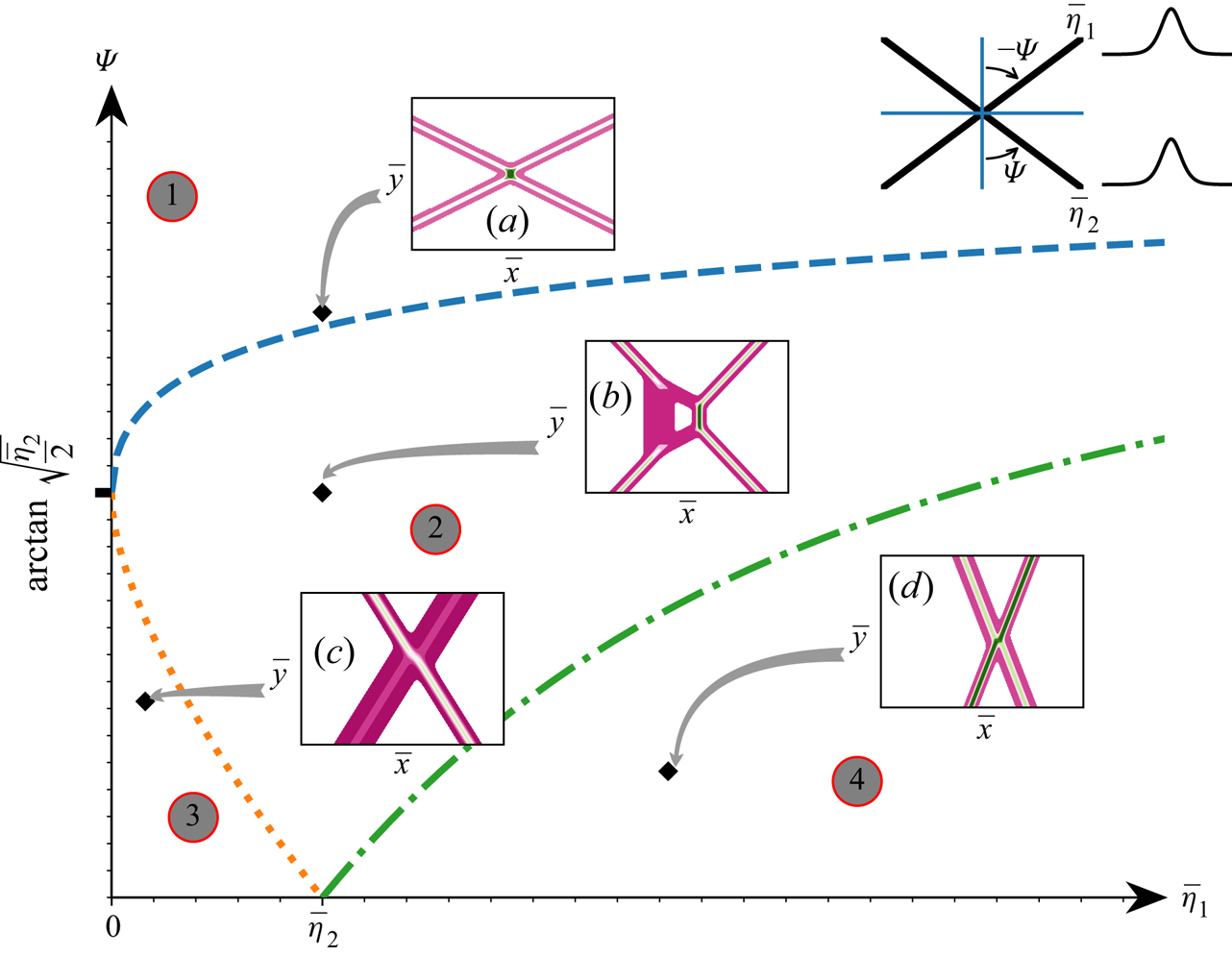
The initial X-shaped pattern, which is composed of two line solitons with amplitudes  $\bar {\eta }_{1,2}$ and inclination angles
 $\pm \varPsi$, is shown in the upper right corner. The
 $\bar {\eta }_1- \varPsi$ plane (for
 $\bar {\eta }_2$ fixed) can be divided into four regions according to evolution patterns of the KP equation which are shown in panels (a)–(d). The boundaries between different regions are given by
 $\sqrt {2\bar {\eta }_1}+\sqrt {2\bar {\eta }_2}=2\tan {\varPsi }$ (blue dashed line),
 $\sqrt {2\bar {\eta }_1}-\sqrt {2\bar {\eta }_2}=2\tan {\varPsi }$ (green dash–dotted line) and
 $\sqrt {2\bar {\eta }_2}-\sqrt {2\bar {\eta }_1}=2\tan {\varPsi }$ (orange dotted line). A similar figure plotted with other parameters can be found in Kao & Kodama (Reference Kao and Kodama2012).

3. Numerical method and boundary treatment
To study the evolution of internal solitary waves, in general, we have to solve the mBL equation numerically. Owing to the finiteness of the computational domain, the boundary condition needs special treatment in some cases to avoid radiated waves from re-entering the domain. For this purpose, a windowing method proposed by Schlatter, Adams & Kleiser (Reference Schlatter, Adams and Kleiser2005) will be used in the subsequent numerical experiments. Its core idea is to divide the solution domain into the interior and the boundary-layer regions in the transverse direction (orthogonal to wave propagation) using a smooth function with compact support, termed the window function. Because analytic solutions to the problem under investigation are usually used in the boundary layers, numerical errors inevitably emanate from junction regions and propagate inwards. However, as these tiny errors propagate with finite speed, little contamination affects the active portion of the wave phenomenon being studied if the domain is large enough considering our relatively short computation time.
We choose  $x$ as the direction of wave propagation and split the unknown
 $\xi$ in (2.24) into two components:
 \begin{equation} \xi = \psi_1+\psi_2\quad \text{with} \ \psi_1=W\xi, \quad \psi_2=(1-W)\xi. \end{equation}
The window function  $W(y)$ is nearly one over some interval (say
 $[-L_y+\varepsilon,L_y-\varepsilon ]$ for a small
 $\varepsilon$) and rapidly decays to zero near two boundaries
 $y=\pm L_y$. Specifically,
 $W(y)$ can be defined as
 \begin{equation} W(y)=\exp\left({-}a \left|\frac{y}{L_y}\right|^{n}\right) , \end{equation}
where  $n=95$ and
 $a=(1.02)^{n}\ln {10}$ are chosen in all computations. It is clear that
 $\psi _1$ and
 $\psi _2$ represent the respective contributions of the interior and boundary-layer regions. Substituting (3.1) into (2.24) yields
 \begin{equation} \psi_{1tt}-c^{2}\Delta\psi_1-\alpha\Delta\psi_{1tt}+\gamma\left[\left(|\boldsymbol{\nabla}\psi_1|^{2}\right)_t+ \psi_{1t}\Delta\psi_1\right]+\beta\boldsymbol{\nabla}\boldsymbol{\cdot} b\boldsymbol{\nabla}\psi_1=G_1+G_2, \end{equation}
where
 \begin{equation} \left.\begin{gathered} G_1=\gamma\left[{-}2\boldsymbol{\nabla}\psi_1\boldsymbol{\cdot}\boldsymbol{\nabla} \psi_{2t}-2\boldsymbol{\nabla}\psi_2\boldsymbol{\cdot}\boldsymbol{\nabla}\psi_{1t}-\psi_{1t}\Delta\psi_2 - \psi_{2t}\Delta\psi_{1}\right],\\ G_2={-}\psi_{2tt}+c^{2}\Delta\psi_2+\alpha\Delta\psi_{2tt}-\gamma\left[\left(|\boldsymbol{\nabla}\psi_2|^{2}\right)_t+ \psi_{2t}\Delta\psi_2\right]-\beta\boldsymbol{\nabla}\boldsymbol{\cdot}b\boldsymbol{\nabla}\psi_2 . \end{gathered}\right\} \end{equation}
In practice, the solution near the boundary is assumed to be a line solitary wave  $\xi _0$ with the explicit expression (2.26a,b). Hence,
 $\psi _2=(1-W)\xi _0$ simplifies the computation of
 $G_2$. Thus, we can enforce doubly periodic boundary conditions for
 $\psi _1$, owing to its exponential decay in all spatial directions, and the pseudo-spectral method is applicable.
We next sketch the numerical scheme for time-dependent simulations of the mBL equation. Following Milewski & Tabak (Reference Milewski and Tabak1999), (3.3) can be rewritten as
 \begin{equation} (1-\alpha\Delta)\psi_{1tt}-c^{2}\Delta\psi_{1} = \mathcal{N}(\psi_{1,2},\partial_t\psi_{1,2},\boldsymbol{\nabla}\psi_{1,2},b), \end{equation}
where  $\mathcal {N}$ includes all the nonlinear terms. Rearranging the operator
 $1-\alpha \varDelta$ and introducing
 \begin{equation} \theta = \left(\frac{\partial}{\partial t} + \text{i}\mathcal{L}\right)\psi_1,\quad \mathcal{L}^{2}=\frac{-c^{2}\varDelta}{1-\alpha\varDelta} , \end{equation}
(3.5) can be simplified to a complex first-order equation,
 \begin{equation} \left(\frac{\partial}{\partial t}-\text{i}\mathcal{L}\right)\theta = \frac{1}{1-\alpha\varDelta} \mathcal{N}(\psi_{1,2},\partial_t\psi_{1,2},\boldsymbol{\nabla}\psi_{1,2},b). \end{equation}
Taking the Fourier transform of the above equation in the spatial variables yields
 \begin{equation} \left(\frac{\partial}{\partial t}-\text{i}\hat{\mathcal{L}}(\boldsymbol{k})\right) \hat{\theta}(\boldsymbol{k},t)=\frac{\mathcal{F}\left[\mathcal{N}(\psi_{1,2},\partial_t\psi_{1,2},\boldsymbol{\nabla}\psi_{1,2},b)\right](\boldsymbol{k},t)}{\mathcal{F}[1-\alpha\varDelta](\boldsymbol{k})},\end{equation}
where both  $\hat {\cdot }$ and
 $\mathcal {F}$ stand for the Fourier transform and
 $\hat {\mathcal {L}}(\boldsymbol {k})$ is the Fourier symbol of the linear operator
 $\mathcal {L}$. The time-evolution equation (3.8) can be numerically advanced using the method of integrating factors coupled with the fourth-order Runge–Kutta scheme for time-stepping. Using the fact that
 $\psi _1$ is real,
 $\psi _1$ and
 $\partial _t\psi _{1}$ can be recovered from
 $$\begin{gather} \widehat{\psi_1}(\boldsymbol{k},t)=\frac{\hat{\theta}(\boldsymbol{k},t)-\hat{\theta}^{*}(-\boldsymbol{k},t)}{\text{i}\left[\hat{\mathcal{L}}(-\boldsymbol{k})+\hat{\mathcal{L}}(\boldsymbol{k})\right]}, \end{gather}$$
 $$\begin{gather}\partial_t\widehat{\psi_1}(\boldsymbol{k},t)=\frac{\hat{\theta}(\boldsymbol{k},t)+\hat{\theta}^{*}(-\boldsymbol{k}, t)}{2}, \end{gather}$$
where the asterisk indicates complex conjugation. It should be pointed out that  $\hat {\psi _1}(\boldsymbol {0},t)$ cannot be recovered from (3.9) because
 $\hat {\mathcal {L}}(\boldsymbol {0})=0$, but instead, it should be updated numerically by integrating (3.10) at
 $\boldsymbol {k}=\boldsymbol {0}$. Finally, when internal solitary waves are chosen as initial conditions, the solution
 $\xi$ given in (2.26a,b) is not a periodic function; therefore, modification is required. We replace
 $\xi$ with
 \begin{equation} \xi={-}\frac{A}{vk}\,\text{tanh}(\boldsymbol{k}\boldsymbol{\cdot}\boldsymbol{r}-vkt)+ \boldsymbol{P}\boldsymbol{\cdot}\boldsymbol{r}, \end{equation}
where  $\boldsymbol {P}$ is a constant vector chosen to keep
 $\xi$ periodic. In the following numerical simulations, dimensional variables are used to mimic the realistic oceanic environment. We pick 75 m as the spatial step in both
 $x$- and
 $y$-directions and 5 s as the temporal step in all computations.
4. Results
4.1. Truncated and partially bent solitary waves
In the ocean, one interesting scenario is the evolution of an internal solitary wave passing through a strait or diffracting off the end of a topographic feature; see those, for instance, in the Strait of Gibraltar (Vlasenko et al. Reference Vlasenko, Sanchez Garrido, Stashchuk, Lafuente and Losada2009). We investigate this problem in the mBL equation and the KP equation, and the results are shown in panels (b) and (e) of figure 3, respectively. We take as initial data the solitary waves in the form of (2.26a,b) and (2.35) with amplitude of  $-20$ m truncated at the ends with a fast cutoff (see figure 3a). In addition, the actual computational domain in the
 $y$-direction is twice as large as shown in the figure to allow for periodicity. A qualitative disparity can be found between these two models where a circular pattern emanates from the end of the truncated nonlinear wave in the mBL equation, compared with a bent dispersive wave in the KP equation. As shown in figure 3(f), the interface fluctuations at section lines
 $y=0$ and
 $12.5$ km also display differences. We claim that this comparison shows the advantage of the isotropic bidirectional model. To put this assertion on a firmer footing and further verify the validity of the mBL equation, we conduct a numerical simulation with the same set-up based on the Massachusetts Institute of Technology general circulation model (MITgcm), which solves the fully nonlinear and non-hydrostatic primitive equations (see Marshall et al. (Reference Marshall, Adcroft, Hill, Perelman and Heisey1997) for an overview of the MITgcm).
(a) Initial internal solitary wave of amplitude  $-20$ m. (b) Snapshot of the wave pattern at
 $t=7500$ s in the mBL equation with a flat bottom. (c) Snapshot of the wave pattern at
 $t=7500$ s in the mBL equation in the presence of
 $y$-dependent topography
 $b(y)$ shown on the far right. (d) Temperature profile in the MITgcm model at
 $t=7500$ s. (e) Snapshot of the wave pattern at
 $t=7500$ s in the KP equation with a flat bottom. (f) Interface fluctuations along section lines
 $y=0$ (bottom) and
 $y=12.5$ km (top) at
 $t=7500$ s.

In the realistic situation, the ocean stratification is continuous; however, the mBL equation derived here is based on the two-layer simplification, which causes difficulty when it is intended to be invoked for the oceanic environment. We propose a layering scheme to establish a connection between continuous and discontinuous vertical density stratifications to circumvent this issue. Note that the KP equation (2.31) has an extension for a continuous stratification (see Yuan et al. (Reference Yuan, Grimshaw, Johnson and Chen2018b) and the references therein), where, in the absence of topographic effects, the significant parameters are given as
 \begin{gather} I\varphi = 3\int_{{-}h^{-}}^{h^{+}}\rho_0 c^{2}\varPhi_z^{3}\, {\rm d}z , \end{gather}
 \begin{gather}I\vartheta = \int_{{-}h^{-}}^{h^{+}}\rho_0 c^{2}\varPhi^{2}\, {\rm d}z , \end{gather}
 \begin{gather}I = 2\int_{{-}h^{-}}^{h^{+}} \rho_0 c \varPhi_z^{2} \, {\rm d}z , \end{gather}
where  $\rho _0(z)$ is the continuous density profile, and the mode
 $\varPhi$ and linear phase speed
 $c$ are obtained by solving the modal problem
 \begin{gather} \left(\rho_0 c^{2}\varPhi_z \right)_z+\rho_0N^{2}\varPhi=0,\quad \text{for}\ -h^{-}< z< h^{+},\end{gather}
 \begin{gather} \varPhi=0,\quad\text{at}\ z={-}h^{-}\ \text{and}\ h^{+},\end{gather}
where  $N$ is the buoyancy frequency defined as
 $N^{2}=-({g}/{\rho _0})({\textrm {d}\rho _0}/{\textrm {d}z})$. In practice, to construct a two-layer fluid system based on a given realistic continuous stratification, the thicknesses
 $h^{\pm }$ and densities
 $\rho ^{\pm }$ can be numerically determined by keeping the main parameters
 $c$,
 $\varphi$,
 $\vartheta$ given in (2.23), (2.32), (2.33) as close as those in the continuous medium (4.1)–(4.5), by virtue of the least squares method. This scheme is able to achieve the kinematic equivalence (approximately) between two-layered and continuous stratifications.
In the MITgcm simulation, the water depth is assumed to be  $300\,$m. The continuous density distribution is shown in figure 1, calculated from the monthly averaged background temperature and salinity profiles (data from the World Ocean Atlas 2013). The kinematically equivalent layering yields
 $h^{+}=83$ m,
 $h^{-}=217$ m and
 $R=\rho ^{+}/\rho ^{-}=0.9983$, which are the parameters used in the following computations of the mBL equation and the KP equation. An important issue here is the preparation of the initial solitary wave in the MITgcm. As the solutions to the mBL equation (2.26a,b) and the KP equation (2.35) do not completely satisfy the primitive equations, an adjustment run is needed. We first insert the line soliton and the corresponding velocity field obtained from solving the mBL equation into the MITgcm and then run the model in the
 $x - z$ plane. We let the program evolve until it reaches a steady state, taken as the initial solitary wave for the MITgcm. Despite quantitative differences, the result of the MITgcm model shows a similar circular refraction pattern as that in the mBL equation (figure 3d versus figure 3b), which confirms the validity of the mBL equation and indicates the failure of the KP equation in some cases. We note that a very recent study by Ryskamp et al. (Reference Ryskamp, Maiden, Biondini and Hoefer2021) based on the KP equation shows a similar pattern (figure 5 in their paper) as our figure 3(e). Thus it is of great interest to revisit their problem based on an isotropic bi-directional model, for instance, the Benney–Luke equation.
In this paper, the modification to the classic Benney–Luke equation is the inclusion of topographic effects. The transverse variation of the topography modulates the wave pattern to some extent, as shown by the comparison between figure 3(b) and figure 3(c). As shown in figure 3(f), the interface fluctuations (denoted as  $\eta$) at section lines
 $y=0$ and
 $12.5$ km imply that the existence of topography leads to an increase in wave amplitude and a decrease in wave speed. Nonetheless, the scales (2.15a–f) used in the derivation indicate that the height of topography is of the same order as the wave amplitude. Thus a significant topography should be used with precaution in numerical computations.
Next, we check the evolution of a partially bent solitary wave, composed of a truncated solitary wave of amplitude  $\eta _0=-30$ m as the middle stem, abruptly extended by two outgoing oblique solitary waves of amplitude
 $\eta _0=-10$ m and bent angles
 $\pm 20^{\circ }$ (see figure 4a). Again, the result illustrates a significant disparity between the KP equation and the mBL equation (figure 4b–c versus figure 4d–e), which further manifests the feature of the isotropic model. The discontinuities at the conjunction regions eventually evolve into two circular diffraction patterns in the mBL equation rather than arched trailing waves in the KP equation. The transverse variation of the topography
 $b(y)$ modifies the waveform, increases its amplitude and slows the propagation speed, akin to figure 3.
(a) Initial internal solitary waves with amplitudes  $\eta _0=-30$ m for the middle stem and
 $\eta _0=-10$ m for oblique branches of bent angles
 $\pm 20^{\circ }$. (b,c) Snapshots of the wave pattern in the KP equation with a flat bottom at
 $t=5400$ and 10 800 s, respectively. (d,e) Snapshots of the wave pattern in the mBL equation with a flat bottom at
 $t=5400$ and 10 800 s, respectively. (f,g) Snapshots of the wave pattern at
 $t=5400$ and 10 800 s, respectively, in the mBL equation in the presence of
 $y$-dependent topography
 $b(y)$ shown on the far right. (h,i) Interface fluctuations at
 $t=10\,800$ s along section lines
 $y=0$ and
 $y=12.5$ km, respectively.

4.2. X-shaped wave–wave interactions
The oblique internal wave–wave interactions exhibit three-dimensional characteristics and likely give rise to peculiar wave patterns, as revealed by numerous observations in the ocean, primarily via satellite images (see, for example Hsu, Liu & Liu Reference Hsu, Liu and Liu2000; Xue et al. Reference Xue, Graber, Romeiser and Lund2014). On this topic, the pioneering work of Miles (Reference Miles1977a,Reference Milesb) classifies the interaction as either ‘strong’ or ‘weak’ depending on the inclination angle between two solitons and theoretically describes ‘Mach reflection’ as the resonant interaction. In recent years, a series of progress was made by Chakravarty & Kodama (Reference Chakravarty and Kodama2008, Reference Chakravarty and Kodama2009, Reference Chakravarty and Kodama2013), who proposed a method to construct multi-soliton solutions to the KP equation. These solutions manifest themselves as an arbitrary number of line solitons in the far field and a novel wave pattern owing to the wave interaction in the near field. Based on their method, the interaction patterns observed in reality can be easily reproduced in theory (if applicable) via counting the number of solitons in the far field and measuring the amplitude and slope of each soliton. Using their results and the variable-coefficient KP equation, Yuan et al. (Reference Yuan, Grimshaw, Johnson and Wang2018a) investigated the topographic effects on the so-called V-shaped internal wave–wave interactions, which abound in oceans. In addition to the V-shaped interactions, the X-shaped internal wave–wave interactions (see the upper right corner of figure 2) are also very likely to occur in oceans, albeit few studies have specifically focussed on this type of interaction.
We first briefly introduce the work of Chakravarty & Kodama (Reference Chakravarty and Kodama2008, Reference Chakravarty and Kodama2009, Reference Chakravarty and Kodama2013). Note that the KP equation (2.31) can be transformed to the canonical form
 \begin{equation} \left(4\bar{\eta}_{\bar{t}}+6\bar{\eta}\bar{\eta}_{\bar{x}}+\bar{\eta}_{\bar{x}\bar{x}\bar{x}}\right)_{\bar{x}}+3\bar{\eta}_{\bar{y}\bar{y}}=0 , \end{equation}
where new variables with overline are defined as
 \begin{equation} t = \left(\sqrt{\frac{27\vartheta}{2c^{3}}}\right)\bar{t}, \quad x-ct=\left(\sqrt{\frac{6\vartheta}{c}}\right)\bar{x}, \quad y=\left(\sqrt{\frac{6\vartheta}{c}}\right)\bar{y}, \quad \eta=\left(\frac{c}{\varphi}\right)\bar{\eta}. \end{equation}
The soliton solution to (4.6) in the Wronskian form is represented by
 \begin{equation} \bar{\eta} = 2 (\ln \tau)_{\bar{x}\bar{x}} , \end{equation}
where  $\tau (\bar {x},\bar {y},\bar {t})={Wr}(f_1,f_2,\dots,f_N)$, and Wr denotes the Wronskian of the functions
 $f_n$, which can be expressed as a sum of exponential functions, for
 $n=1,2,\ldots,N$,
 \begin{equation} f_n = \sum_{m=1}^{M}\, a_{nm}\exp{(\varTheta_{m})} \quad\text{with}\ \varTheta_m = \sigma_{m} \bar{x} + \sigma_{m}^{2} \bar{y} - \sigma_{m}^{3} \bar{t} . \end{equation}
Obviously, the soliton solution depends on  $M$ (
 $>N$) real parameters, ordered as
 $\sigma _1<\sigma _2<\cdots < \sigma _{M}$, and constants
 $a_{nm}$ forming an
 $N\times M$ coefficient matrix
 $\mathbb {A}$ with
 $\textrm {rank}(\mathbb {A})=N$. Suppose we denote by
 $\chi (j_1,j_2,\ldots,j_N)$ the
 $N\times N$ minor of
 $\mathbb {A}$ obtained from columns
 $1\leqslant j_1<\cdots < j_N\leqslant M$, then to ensure a non-singular solution (4.8), all the
 $N\times N$ minors of
 $\mathbb {A}$ should be non-negative, i.e.
 $\chi (j_1,j_2,\ldots,j_N)\geqslant 0$. It was proved by Chakravarty & Kodama (Reference Chakravarty and Kodama2009) that as
 $\bar {y} \to \infty$, there exist
 $N$ line solitons, while as
 $\bar {y} \to -\infty$, there are
 $M-N$ line solitons. For example, for
 $M=2$ and
 $N=1$, one line soliton exists as either
 $\bar {y} \to -\infty$ or
 $\bar {y} \to \infty$, and the
 $N\times M$ matrix
 $\mathbb {A}=(1,a)$, where
 $a>0$ is a constant determining the location of the wave. Subsequently,
 $\tau (\bar {x},\bar {y},\bar {t})$ can be defined as
 \begin{equation} \tau=\exp(\varTheta_{1}) + a \exp(\varTheta_{2}), \end{equation}
and substituting (4.10) into the solution (4.8) yields
 \begin{equation} \bar{\eta}=\frac{\bar{k}^{2}}{2}\,\text{sech}^{2} \left(\frac{\bar{k}\bar{x}+\bar{l}\bar{y}-\omega\bar{t}+\ln a}{2}\right), \end{equation}
where
 \begin{equation} \bar{k} = \sigma_2 - \sigma_1,\quad \bar{l}=\sigma_2^{2}-\sigma_1^{2},\quad \omega=\sigma_2^{3}-\sigma_1^{3}=\frac{\bar{k}^{4}+3\bar{l}^{2}}{4\bar{k}} . \end{equation}
Equation (4.11) can be further rewritten in terms of physical variables as
 \begin{equation} \bar{\eta}= \bar{\eta}_0\, \text{sech}^{2} \left[\bar{\varGamma}(\bar{x}+\bar{y}\tan{\varPsi }-\bar{\varpi}\bar{t}+\bar{x}_0)\right], \end{equation}
where
 \begin{equation} \bar{\eta}_0=\frac{\bar{k}^{2}}{2},\quad \bar{\varGamma}=\sqrt{\frac{\bar{\eta}_0}{2}},\quad \bar{\varpi}=\frac{1}{2}\bar{\eta}_0+\frac{3}{4}\tan^{2}{\varPsi},\quad \bar{x}_0=\frac{\ln{a}}{\sqrt{2\bar{\eta}_0}}, \end{equation}
and  $\varPsi$ is the inclination angle of the line soliton measured counterclockwise with respect to the
 $y$-axis. Upon noticing that the spatial scaling factors are the same, the angle
 $\varPsi$ is unchanged under the transformation (4.7a–d), which can be expressed as
 \begin{equation} \tan\varPsi = \frac{\bar{l}}{\bar{k}} = \sigma_1 + \sigma_2 . \end{equation}
In practice, one can easily obtain  $\bar {\eta }_0$ and
 $\varPsi$ from the field observation together with the transformation (4.7a–d), and then
 $\sigma _1$ and
 $\sigma _2$ can be recovered by solving
 $\bar {\eta }_0={(\sigma _2-\sigma _1)^{2}}/{2}$ and (4.15). Eventually, a soliton solution to the KP equation is constructed.
The initial X-shaped wave can be prepared by intersecting two line solitons whose inclination angles with respect to the transverse  $y$-direction are
 $\pm \varPsi$ (see the right upper corner of figure 2). The amplitudes of two solitons, denoted by
 $\eta _1$ and
 $\eta _2$, do not necessarily have to be the same. Based on the aforementioned theory of the KP equation, the evolution of the initial X-shaped wave can be categorised into four types, corresponding to four different regions in the first quadrant of the
 $\eta _1- \varPsi$ plane (for a fixed
 $\eta _2$), as shown in figure 2. No analytic solutions were found to exist on the boundaries between different regions (i.e. the broken lines).
For case (a), we choose  $\eta _1=\eta _2=-15$ m, which can be transformed to
 $\bar {\eta }_1=\bar {\eta }_2=0.17$ based on the scaling (4.7a–d), and the boundary separating case (a) from other cases is depicted as
 $\sqrt {2\bar {\eta }_1}+\sqrt {2\bar {\eta }_2}=2\tan {\varPsi _0}$ that gives the critical angle
 $\varPsi _0\approx 30^{\circ }$. Here we choose
 $\varPsi =33^{\circ }>\varPsi _0$. Snapshots of the wave pattern at different times are shown in figure 5, where the most remarkable features are the phase shift in the interaction zone (see a zoom-in in figure 6) and the trailing waves arising from the self-adjustment process. When the results are scrutinised, the discrepancy in wave amplitude between the KP equation and the mBL equation is conspicuous, and the latter is rendered with a slightly smaller amplitude (see figure 5h–i or figure 6d). It is shown in figure 5(h) that the variation of bottom topography in the direction of internal wave propagation augments the wave amplitude in the interaction zone, and no obviously disparate trailing waves are generated.
(a) Initial X-shaped wave with amplitudes  $\eta _1=\eta _2=-15$ m and inclination angle
 $\varPsi =33^{\circ }$. (b,c) Snapshots of the wave pattern in the KP equation with a flat bottom at
 $t=1.5\times 10^{4}$ and
 $3.0\times 10^{4}$ s, respectively. (d,e) Snapshots of the wave pattern in the mBL equation with a flat bottom at
 $t=1.5\times 10^{4}$ and
 $3.0\times 10^{4}$ s, respectively. (f,g) Snapshots of the wave patterns at
 $t=1.5\times 10^{4}$ and
 $3.0\times 10^{4}$ s, respectively, in the mBL equation with
 $x$-dependent topography
 $b(x)$ shown on the extreme right. (h,i) Interface fluctuations at
 $t=3.0\times 10^{4}$ s along section lines
 $y=0$ and
 $y=5$ km, respectively. For the results of the mBL equation with topography, the actual computational domain in the
 $x$-direction is twice that shown in the figure to allow for periodicity.

(a–c) Close-ups of the interaction zone of figure 5 at  $t=3.0\times 10^{4}$ s. The phase shifts (denoted by
 $\delta x$) for the KP equation, the mBL equation and the mBL equation with topography
 $b(x)$ are respectively highlighted. (d) Time series of the wave amplitude at the intersection point computed with different models, together with the asymptotic prediction (blue dashed line).

In solution (4.8), two branches of the initial X-shaped wave are described by two sets of parameters for case (a),  $(\sigma _1,\sigma _2)=(-0.61,-0.04)$ and
 $(\sigma _3,\sigma _4)=(0.04,0.61)$. Because
 $\bar {\eta }_1=\bar {\eta }_2$, the phase shifts (denoted by
 $\bar {\delta x}$ in the transformed plane (4.7a–d)) for the upper and lower branches turn out to be the same, which can be predicted by
 \begin{equation} \bar{\delta x} = \frac{\varTheta_{12}}{\sigma_2-\sigma_1}, \quad \varTheta_{12} ={-}\ln \varDelta_0, \quad 0<\varDelta_0=\frac{(\sigma_3-\sigma_2)(\sigma_4-\sigma_1)}{(\sigma_4-\sigma_2)(\sigma_3-\sigma_1)}<1, \end{equation}
leading to  $\delta x=366$ m in the original variables. However, the numerical results are
 $\delta x=326$ m for the KP equation,
 $\delta x=413$ m for the mBL equation and
 $\delta x=439$ m for the mBL equation with the topography
 $b(x)$ (see figure 6), and plausibly all of them can be considered as good approximations. Note that the phase shift is independent of time. Similarly, this theoretical result also predicts the wave amplitude in the interaction zone, namely
 \begin{equation} \bar{\eta}_{{max}} = \bar{\eta}_1 + \bar{\eta}_2 + 2 \frac{1-\sqrt{\varDelta_0}}{1+\sqrt{\varDelta_0}}\sqrt{\bar{\eta}_1 \bar{\eta}_2} , \end{equation}
which gives  $\eta _{{max}}=-41$ m after being converted to the original variables. It is shown in figure 6(d) that the numerical result of the KP equation asymptotically approaches the theoretical prediction. However, the numerical solution to the mBL equation is still a bit off the theoretical value after 6 h of evolution.
Next, we investigate case (b) by illuminating a quantitative example of the schematic in figure 2(b). Here we choose the amplitudes  $\eta _1=\eta _2=-15$ m and inclination angle
 $\varPsi =25^{\circ }$. As time evolves, a separation commences from the interaction zone resulting in an opening isosceles trapezium (figures 7 and 8). Note that the equivalence of the leg lengths arises from the initial setting
 $\eta _1=\eta _2$. Considering numerical errors, we do not detect perceptible differences in waveform between the KP equation and the mBL equation, though there is a slight discrepancy in wave amplitude. As in case (a), it is clear that the shoaling can augment the wave amplitude; see the comparisons in figure 7(h–i).
(a) Initial X-shaped pattern with amplitudes  $\eta _1=\eta _2=-15$ m and inclination angle
 $\varPsi =25^{\circ }$. (b,c) Snapshots of the wave pattern in the KP equation with a flat bottom at
 $t=9\times 10^{3}$ and
 $1.8\times 10^{4}$ s, respectively. (d,e) Snapshots of the wave pattern in the mBL equation with a flat bottom at
 $t=9\times 10^{3}$ and
 $1.8\times 10^{4}$ s, respectively. (f,g) Snapshots of the wave pattern at
 $t=9\times 10^{3}$ and
 $1.8\times 10^{4}$ s, respectively, in the mBL equation with
 $x$-dependent topography
 $b(x)$ shown under panel (g). (h,i) Interface fluctuations at
 $t=1.8\times 10^{4}$ s along section lines
 $y=0$ and
 $y=5$ km, respectively. For the results of the mBL equation with topography, the actual computational domain in the
 $x$-direction is twice that shown in the figure to allow for periodicity.

(a–c) Close-ups of the interaction zone of figure 7 at  $t=1.8\times 10^{4}$ s. The lengths of the middle stem
 $L_s$ and the widths of the generated ‘trapezium’
 $L_d$ are highlighted for the KP equation, the mBL equation and the mBL equation with topography
 $b(x)$. (d,e) Time series of
 $L_s$ and
 $L_d$ computed with different models along with the theoretically predicted values.

In the framework of the KP equation, the theoretical descriptions of case (b) are much more complicated than those of case (a), whose behaviours within the interaction zone depend only on several parameters determined by the initial waves. It is not difficult to see that  $N=2$ and
 $M=4$ for case (b), and therefore the coefficient matrix
 $\mathbb {A}$ can be represented as
 \begin{equation} \mathbb{A}=\left( \begin{array}{cccc} 1 & 0 & -a & -b \\ 0 & 1 & c & d \end{array} \right), \end{equation}
where  $a,b,c,d>0$ are free parameters determining the locations of solitons, their phase shifts and the onset of the trapezium pattern. The minors of
 $\mathbb {A}$ satisfy
 $\chi (j_1,j_2)\geqslant 0$ to ensure the existence of non-singular solutions and particularly,
 $bc-ad>0$. In this situation, the initial two branches can be delineated by the pairs
 $(\sigma _1,\sigma _3)$ and
 $(\sigma _2,\sigma _4)$, as illustrated in figure 8(a). These parameters can be easily calculated from the amplitudes and inclination angles of the given initial data. Actually, using (4.11) and (4.15), one obtains
 $(\sigma _1,\sigma _2,\sigma _3,\sigma _4)=(-0.52,-0.06,0.06,0.52)$ for this example. The phase shift of the upper right branch (
 $\bar {x}>0$ and
 $\bar {y}\gg 0$) is represented by
 \begin{equation} \varTheta_{13}^{+} = \ln \frac{\sigma_4-\sigma_1}{\sigma_4-\sigma_3} - \ln \frac{\digamma}{b} , \end{equation}
where  $\digamma =\chi (3,4)=bc-ad$, while for the lower left branch (
 $\bar {x}<0$ and
 $\bar {y}\ll 0$),
 \begin{equation} \varTheta_{13}^{-} = \ln \frac{\sigma_2-\sigma_1}{\sigma_3-\sigma_2} - \ln c. \end{equation}
Similarly, the phase shifts for the upper left branch ( $\bar {x}<0$ and
 $\bar {y}\gg 0$) and lower right branch (
 $\bar {x}>0$ and
 $\bar {y}\ll 0$) read
 \begin{equation} \varTheta_{24}^{+} = \ln \frac{\sigma_3-\sigma_2}{\sigma_4-\sigma_3} - \ln \frac{\digamma}{c} , \quad \varTheta_{24}^{-} = \ln \frac{\sigma_2-\sigma_1}{\sigma_4-\sigma_1} - \ln b , \end{equation}
respectively. Thus, in theory, the phase shifts of the two branches are  $\varTheta _{13}=\varTheta _{13}^{+}-\varTheta _{13}^{-}$ and
 $\varTheta _{24}=\varTheta _{24}^{+}-\varTheta _{24}^{-}$, which depend not only on
 $\sigma _j$ but also on the free parameters
 $a,b,c,d$. Nonetheless, the phase shift along the
 $\bar {y}$-direction is conserved because
 \begin{equation} \varTheta_{13}^{+} + \varTheta_{24}^{-}= \varTheta_{24}^{+} + \varTheta_{13}^{-} = \ln \frac{\sigma_2-\sigma_1}{\sigma_4-\sigma_3} - \ln \digamma . \end{equation}
In contrast to the phase shift depending on free parameters, we can determine the length of the stem  $\bar {L}_s$, the asymptotic amplitude of the stem
 $\bar {\eta }_{\textrm {max}}$ and the width of the opening trapezium
 $\bar {L}_d$, using the properties of initial waves (see figure 8). Here the upper right branch is described by
 $(\sigma _1,\sigma _3)$ and the stem by
 $(\sigma _1,\sigma _4)$. Therefore, the ridges of these two parts are given by
 $\varTheta _{1}=\varTheta _{3}$ and
 $\varTheta _{1}=\varTheta _{4}$, respectively. Recalling the definition of
 $\varTheta _{j}$ given in (4.9), one obtains
 \begin{gather} \bar{x} + (\sigma_3+\sigma_1)\bar{y}=\left(\sigma_1^{2}+\sigma_1\sigma_3+\sigma_3^{2}\right)\bar{t} , \end{gather}
 \begin{gather}\bar{x} = \left(\sigma_1^{2}+\sigma_1\sigma_4+\sigma_4^{2}\right)\bar{t} , \end{gather}
upon noting that  $\sigma _1+\sigma _4=0$ and
 $\sigma _2+\sigma _3=0$. The wave pattern is symmetric about the
 $x$-axis given
 $\eta _1=\eta _2$, and thus the length of the stem
 $\bar {L}_s=2\bar {y}$, where
 $\bar {y}$ indicates the location of the intersection point. A simple manipulation of (4.23)–(4.24) yields
 \begin{equation} \bar{L}_s=2\sigma_3 \bar{t} . \end{equation}
In the long-time evolution, the amplitude of the stem approaches the asymptotic value given by
 \begin{equation} \bar{\eta}_{{max}} = \tfrac{1}{2}(\sigma_4-\sigma_1)^{2} . \end{equation}
The width of the opening trapezium,  $\bar {L}_d$, depends on the phase speed discrepancy between the stem and the other parallel side delineated by
 $(\sigma _2,\sigma _3)$, which takes the form
 \begin{equation} \bar{L}_d = \left(\sigma_4^{2}-\sigma_3^{2}\right)\bar{t} . \end{equation}
It is clear that both the predicted  $\bar {L}_s$ and
 $\bar {L}_d$ are linear functions of time, and comparisons between the theoretical predictions and numerical simulations of different models are illustrated in figure 8(d–e). These comparisons are generally in good agreement, although slight differences, partly attributed to insufficient evolution time, are inevitable. This is shown, for example, by the gap between the amplitude of the stem
 $\eta \approx -44$ m (figure 7h) at the termination time of the computation
 $t=1.8\times 10^{4}$ s and the predicted asymptotic value
 $\eta _{max}=-49$ m.
From the physical point of view, case (c) and case (d) are of the same dynamical and kinematical properties by a simple reversal of the  $y$-axis; thus, we confine ourselves to case (c). Here we choose wave amplitudes
 $\eta _1=-5$ m (denoted by
 $(\sigma _2,\sigma _3)$) and
 $\eta _2=-15$ m (denoted by
 $(\sigma _1,\sigma _4)$), together with the inclination angle
 $\varPsi =5^{\circ }$ which is smaller than the critical angle
 $\varPsi _0=\textrm {atan}(\sqrt {\bar {\eta }_2/2}-\sqrt {\bar {\eta }_1/2})\approx 7^{\circ }$. It is calculated that
 $(\sigma _1,\sigma _2,\sigma _3,\sigma _4)=(-0.25,-0.21,0.12,0.33)$ based on the transformation (4.7a–d). By letting
 $\varTheta _1=\varTheta _4$ and
 $\varTheta _2=\varTheta _3$, one obtains
 \begin{equation} \left.\begin{gathered} \bar{x} + (\sigma_1+\sigma_4)\bar{y} = (\sigma_1^{2}+\sigma_1\sigma_4+\sigma_4^{2})\bar{t},\\ \bar{x} + (\sigma_2+\sigma_3)\bar{y} = (\sigma_2^{2}+\sigma_2\sigma_3+\sigma_3^{2})\bar{t}, \end{gathered}\right\} \end{equation}
and thus the location of the intersection point can be expressed as
 \begin{gather} \bar{L}_x=\frac{7(\sigma_1+\sigma_4)^{2}+(\sigma_3-\sigma_2)^{2}-8\sigma_1\sigma_4}{8}\,\bar{t} = \frac{\bar{\eta}_1+\bar{\eta}_2+3\tan^{2}\varPsi}{4}\,\bar{t}, \end{gather}
 \begin{gather}\bar{L}_y=\frac{(\sigma_1^{2}+\sigma_1\sigma_4+\sigma_4^{2})-(\sigma_2^{2}+\sigma_2\sigma_3+\sigma_3^{2})}{(\sigma_1+\sigma_4)-(\sigma_2+\sigma_3)}\,\bar{t} =\frac{\bar{\eta}_2-\bar{\eta}_1}{4\tan\varPsi}\,\bar{t}. \end{gather}
The intersection point moves in the positive  $y$-direction owing to
 $\eta _2>\eta _1$ (see figure 9). The numerical results of
 $L_y$ for model equations are illustrated in figure 10, which show good agreement with the theoretical prediction. The phase shifts for the two branches are
 \begin{equation} \overline{\delta x}_{ij} ={-}\frac{1+\ln \varDelta_0}{\sigma_j-\sigma_i}, \quad \varDelta_0=\frac{(\sigma_4-\sigma_2)(\sigma_3-\sigma_1)}{(\sigma_4-\sigma_3)(\sigma_2-\sigma_1)}, \end{equation}
where the subscript  $(i,j)$ is either
 $(1,4)$ or
 $(2,3)$, representing the branches of the initial X-shaped wave. As shown in figure 10, the phase shifts of the branch characterised by
 $(\sigma _1,\sigma _4)$ are
 $\delta x_{14}=1.1$ km,
 $0.9$ km and
 $1.0$ km for the KP equation, the mBL equation and the mBL equation with topography, respectively, in comparison with
 $\delta x_{14}=1.0$ km predicted by (4.31a,b). Similarly, the numerical results
 $\delta x_{23}=1.3$ km,
 $1.4$ km,
 $1.4$ km for the three models are close to the theoretical prediction
 $\delta x_{23}=1.7$ km for the branch
 $(\sigma _2,\sigma _3)$.
(a) Initial X-shaped pattern with amplitudes  $\eta _1=-5$ m,
 $\eta _2=-15$ m and inclination angle
 $\varPsi =5^{\circ }$. (b,c) Snapshots of the wave pattern in the KP equation with a flat bottom at
 $t=2.4\times 10^{4}$ and
 $4.8\times 10^{4}$ s, respectively. (d,e) Snapshots of the wave pattern in the mBL equation with a flat bottom at
 $t=2.4\times 10^{4}$ and
 $4.8\times 10^{4}$ s, respectively. (f,g) Snapshots of the wave pattern at
 $t=2.4\times 10^{4}$ and
 $4.8\times 10^{4}$ s, respectively, in the mBL equation with
 $x$-dependent topography
 $b(x)$ shown under panel (g). (h,i) Interface fluctuations at
 $t=4.8\times 10^{4}$ s along section lines
 $y=0$ and
 $y=16$ km, respectively. For the results of the mBL equation with topography
 $b(x)$, the actual computational domain in the
 $x$-direction is twice that shown in the figure to allow for periodicity.

(a–c) Close-ups of the interaction zone of figure 9 at time  $t=4.8\times 10^{4}$ s. The phase shifts
 $\delta x_{14}$ and
 $\delta x_{23}$ of the two branches and the location of the intersection point in the
 $y$-direction
 $L_y$ are highlighted for the KP equation, the mBL equation and the mBL equation with topography
 $b(x)$, respectively. (d) Time series of
 $L_y$ computed with different models together with the theoretically predicted values.

4.3. Truncated X-shaped wave–wave interactions
Because the cases mentioned above focus on the central parts of wave interaction zones, which are of great interest for some scenarios, we apply a windowing method in computations. As a consequence, the propagation of waves in the  $y$-direction is limited. Nevertheless, the realistic ocean should be considered open for internal waves, although the along-crest width can be several hundred kilometres long. Thus, it is informative to investigate the cases in which waves can propagate freely in all horizontal directions. To illustrate this circumstance, we show in figure 11 a radar image photographed in the South China Sea. The subsequent computations display evolutions of initial X-shaped internal waves in an open sea.
An NOAA-20 VIIRS satellite image taken on 16 May 2020, with the left-bottom corner located at  $20.1228^{\circ }\textrm {N}$,
 $115.6389^{\circ }\textrm {E}$ and the right-top at
 $21.61^{\circ }\textrm {N}$,
 $117.133^{\circ }\textrm {E}$.

The set-ups are the same as those in the previous three cases except that an envelope locally confined in the  $y$-direction is imposed on the initial X-shaped waves. Figures 12–15 demonstrate the time evolutions of these truncated patterns. We note an important consequence immediately that the coherent wave–wave interaction patterns (see figures 5–10) are disrupted owing to dispersive effects. After the initial launch, two front edges of the truncated wave begin to collapse and spread in the
 $y$-direction at the cost of decreasing the wave amplitude from the periphery to centre gradually. Meanwhile, the
 $y$-components of the propagation velocities of the two initial waves are opposite. As a result, the intersection zone moves towards the front edges of the pattern, which finally manifests as a leading wave connected by two arched trailing branches. Another significant feature is the post-interaction waves, especially the trailing waves of opposite polarity (waves of positive displacement with red colour in figures 12–15), whose emergence can be explained by mass conservation (Yuan et al. Reference Yuan, Grimshaw, Johnson and Chen2018b).
(a) Initial truncated X-shaped pattern with amplitudes  $\eta _1=\eta _2=-15$ m and inclination angle
 $\varPsi =33^{\circ }$; same as those in figure 5. (b,c) Snapshots of the wave pattern in the KP equation with a flat bottom at
 $t=4.5\times 10^{4}$ and
 $9.0\times 10^{4}$ s, respectively. (d,e) Snapshots of the wave pattern in the mBL equation with a flat bottom at
 $t=4.5\times 10^{4}$ and
 $9.0\times 10^{4}$ s, respectively. (f,g) Snapshots of the wave pattern at
 $t=4.5\times 10^{4}$ and
 $9.0\times 10^{4}$ s, respectively, in the mBL equation with
 $x$-dependent topography
 $b(x)$ shown under panel (g). (h,i) Interface fluctuations at
 $t=9.0\times 10^{4}$ s along section lines
 $y=0$ and
 $y=40$ km, respectively. For the results of the mBL equation with topography
 $b(x)$, the actual computational domain in the
 $x$-direction is twice that shown in the figure to allow for periodicity.

As waves can propagate freely in all horizontal directions, the discrepancies between the KP and mBL equations are evident. One of the most striking differences is the opening degree of trailing waves. It can be seen from panels (b–g) of figures 12, 13 and 15 that waves branch at wider angles in the KP equation, attributing to its anisotropic nature. Moreover, wave amplitudes given by the two equations are significantly different, even a difference of double, as shown in figure 13(h). To put the validity of the mBL equation on a firmer footing, again, we conduct a comparison with the MITgcm model, as illustrated in figure 14, which verifies the use of the mBL equation as a better approximation to the full Euler equations for some cases of practical relevance. These results showcase, to a considerable extent, the advantage of the isotropic property of the mBL equation. Note that the topographic effects play a more significant role in modulating the characteristics of wave evolution, not only the waveform but also the wave amplitude and propagation speed (see panels (h) and (i) of figures 12, 13, 15), compared with the previous three cases. To further examine the effect of bottom gradients, we illustrate two typical cases in figure 16 where truncated X-shaped waves propagate over the shoaling topography superposed by submarine canyon and plateau. Examples are motivated by the realistic ocean topography, such as the Hudson Canyon. It is clear that the canyon (plateau) slightly accelerates (slows) the wave propagation on the shoaling topography, engendering a distortion along the crest where small-amplitude waves emanate from, thereby reshaping wave patterns and altering wave amplitudes.
(a) Initial truncated X-shaped pattern with amplitudes  $\eta _1=\eta _2=-15$ m and inclination angle
 $\varPsi =25^{\circ }$; same as those in figure 7. (b,c) Snapshots of the wave pattern in the KP equation with a flat bottom at
 $t=4.5\times 10^{4}$ and
 $9.0\times 10^{4}$ s, respectively. (d,e) Snapshots of the wave pattern in the mBL equation with a flat bottom at
 $t=4.5\times 10^{4}$ and
 $9.0\times 10^{4}$ s, respectively. (f,g) Snapshots of the wave pattern at
 $t=4.5\times 10^{4}$ and
 $9.0\times 10^{4}$ s, respectively, in the mBL equation with
 $x$-dependent topography
 $b(x)$ shown under panel (g). (h,i) Interface fluctuations at
 $t=9.0\times 10^{4}\,$s along section lines
 $y=0$ and
 $y=40$ km, respectively. For the results of the mBL equation with topography
 $b(x)$, the actual computational domain in the
 $x$-direction is twice that shown in the figure to allow for periodicity.

(a,b) Horizontal views of the temperature profile in the MITgcm simulation at  $t=4.5\times 10^{4}$s and
 $t=9.0\times 10^{4}$ s, respectively. Note that the initial waves are the same as those in figure 13(a). (c,d) Comparisons of the interface fluctuation at
 $t=4.5\times 10^{4}$ s and
 $t=9.0\times 10^{4}$ s, respectively, along the section line
 $y=0$.

(a) Initial truncated X-shaped pattern with amplitudes  $\eta _1=-5$ m,
 $\eta _2=-15$ m and inclination angle
 $\varPsi =5^{\circ }$; same as those in figure 9. (b,c) Snapshots of the wave pattern in the KP equation with a flat bottom at
 $t=4.5\times 10^{4}$ and
 $9.0\times 10^{4}$ s, respectively. (d,e) Snapshots of the wave pattern in the mBL equation with a flat bottom at
 $t=4.5\times 10^{4}$ and
 $9.0\times 10^{4}$ s, respectively. (f,g) Snapshots of the wave pattern at
 $t=4.5\times 10^{4}$ and
 $9.0\times 10^{4}$ s, respectively, in the mBL equation with
 $x$-dependent topography
 $b(x)$ shown under panel (g). (h,i) Interface fluctuations at
 $t=9.0\times 10^{4}$ s along section lines
 $y=0$ and
 $y=40$ km, respectively. For the results of the mBL equation with topography
 $b(x)$, the actual computational domain in the
 $x$-direction is twice that shown in the figure to allow for periodicity.

Initial waves, the same as those in figure 13(a), evolve over the shoaling topography superposed by bottom canyon (a) and plateau (b). (c,d) Snapshots of horizontal wave patterns at time  $t=9.0\times 10^{4}$ s over canyon- and plateau-type topographies. (e,f) Interface fluctuations at
 $t=9.0\times 10^{4}$ s along section lines
 $y=0$ and
 $y=40$ km.

5. Concluding remarks
In this paper, the mBL equation has been derived for internal waves in a two-fluid system with the rigid-lid approximation and variable bottom topography. The model features the isotropic and bi-directional nature and can be numerically implemented to study oblique internal wave–wave interactions, as well as the topographic effects on wave propagation. It is well known that the KP equation is the most widely used model in the context of horizontally two-dimensional internal waves, and indeed, it has a large range of validity inherited from its parent, the KdV equation. Nonetheless, we argue that in some general scenarios, the mBL equation presents more accurate results than the KP equation, which is attributed to the characteristics of isotropy and bi-directional propagation held by the former model. These characters can be easily understood from the linear dispersion relation. For a monochromatic wave with the wavenumber  $\boldsymbol {k}=(k_x,k_y)$ and frequency
 $\omega$, in the absence of bottom topography, the dispersion relations for the KP equation (2.31) and the mBL equation (2.24) read
 \begin{equation} \omega ={-}\vartheta k_x^{3} + ck_x + \frac{c}{2}\frac{k_y^{2}}{k_x}, \quad \omega^{2} = \frac{c^{2} |\boldsymbol{k}|^{2}}{1+\alpha |\boldsymbol{k}|^{2}} , \end{equation}
respectively. It is clear that for the mBL equation, the wave frequency depends entirely on the modulus of the wavenumber vector, and the dispersion relation is hence isotropic, in contrast to the KP equation. However, the corresponding group velocities are given by
 \begin{equation} \left.\begin{gathered} \boldsymbol{\nabla} \omega = \left(-\left(3\vartheta k_x^{2} + \frac{c}{2}\frac{k_y^{2}}{k_x^{2}}\right)+c, \frac{ck_y}{k_x} \right) \quad \text{for the KP equation} , \\ \boldsymbol{\nabla} \omega = \left(\frac{ck_x}{|\boldsymbol{k}|\left(1+\alpha|\boldsymbol{k}|^{2}\right)^{3/2}}, \frac{ck_y}{|\boldsymbol{k}|\left(1+\alpha|\boldsymbol{k}|^{2}\right)^{3/2}}\right) \quad \text{for the mBL equation} . \end{gathered}\right\} \end{equation}
It follows that long waves in the KP equation always propagate towards the positive  $x$-direction considering
 $k_y\ll k_x\ll 1$; however, there is no preferred direction of propagation for the mBL equation.
The advantage of the mBL equation over the KP equation is confirmed by the results of the MITgcm model, which solves the full Navier–Stokes equations and has been extensively used to simulate internal waves in a realistic oceanic environment; see Vlasenko, Guo & Stashchuk (Reference Vlasenko, Guo and Stashchuk2012) amongst many others. The fact that the stratification in the ocean is continuous inspires us to propose a layering scheme to allow the mBL equation derived in the two-layer fluid to model internal waves in a continuous stratification, at least in the sense of kinematical equivalence. This is achieved by matching the primary parameters of the KP equation derived from the mBL equation with those of the KP equation related to a continuous stratification. Note that this layering scheme is of practical interest. However, we should caution that any attempt to approximate a continuous stratification by two-layer configuration raises concern about the possible energy transfer among internal gravity modes, which is absent in the two-layer system with the rigid-lid approximation. Moreover, a vortex sheet between successive layers incurred by the layering scheme is inevitable, and thus an evaluation on the influence of this deceptive vortex needs to be conducted.
Although oblique internal wave–wave interactions frequently occur in oceans, few studies were focused on this topic. In the present paper, following the previous work on V-shaped internal solitons (Yuan et al. Reference Yuan, Grimshaw, Johnson and Wang2018a), another type of oblique soliton interaction, the evolution of an initial X-shaped pattern, has been thoroughly investigated. Unlike the diffraction of a truncated solitary wave and the evolution of a partially bent solitary wave, the oblique interactions of X-shaped internal waves show a similarity between the mBL equation and the KP equation, and no perceptible disparities emerge except for slight differences in amplitude. It is striking that the KP equation does an excellent job of describing the dynamics, which may be attributed to the particularity of the problem under study, limiting the free propagation of waves in the  $y$-direction. In reality, the evolution can be classified into three regimes by the amplitudes and inclination angles of the two branches, where peculiar patterns have been presented, for instance, phase shifts and generation of the trapezium. However, when waves are allowed to propagate freely in the
 $y$-direction, which simulates internal waves in the open ocean, the aforementioned peculiar wave patterns are thoroughly disrupted. Instead, a leading wave is followed by two curved trailing branches between which there exist wave trains of opposite polarity. Moreover, in these scenarios, the discrepancies between the KP equation and the mBL equation are conspicuous, and the topographic effects become significant in modulating the wave evolution.
In this paper, we modify the classic Benney–Luke equation by including topographic effects. In the derivation, the topography is assumed to be of the same order as the wave amplitude. Hinging on this premise, we point out that the shoaling topography and the topography with transverse variations can decrease the wave speed, augment the wave amplitude and modulate the waveform. Nonetheless, a large amount of observational data imply that large topography can modulate wave propagation to a large extent. This scenario is excluded from the present paper owing to the smallness assumption on bottom topography in the mBL equation. The effects of large topography on internal wave propagation are of great interest and merit further exploration. In addition, Shimizu & Nakayama (Reference Shimizu and Nakayama2017) studied the effects of the Earth's rotation and undersea topography on oblique interactions between internal solitary waves in the Andaman Sea. They found that the Earth's rotation has little impact on oblique wave–wave interactions. Considering the low latitude ( ${\sim }9^{\circ }\textrm {N}$) they investigated, their work inspires us to explore further the influence of the Earth's rotation at high latitudes, say the South China Sea (
 ${\sim }22^{\circ }\textrm {N}$), one of the hot-spot regions for studying internal waves, or even the Weddell Sea (
 ${\sim }75^{\circ }\textrm {S}$), as shown by Robertson (Reference Robertson2001).
Funding
This work was supported by the National Natural Science Foundation of China (Nos. 11911530171, 11772341, 42006016), the key program of the National Natural Science Foundation of China (Nos. 12132018, 91958206), the Strategic Priority Research Program of the Chinese Academy of Sciences (No. XDB22040203), the Natural Science Foundation of Shandong Province (No. ZR2020QD063) and the China Postdoctoral Science Foundation (No. 2019M660167).
Declaration of interests
The authors report no conflict of interest.