



1. Introduction
Hypersonic flight and atmospheric reentry represent some of the most challenging environments in aerospace engineering (Leyva Reference Leyva2017). During low-altitude hypersonic flight or atmospheric reentry, the extreme free-stream conditions of high Reynolds numbers, high Mach numbers and high stagnation enthalpies result in high-enthalpy hypersonic turbulent boundary layers (HE-TBLs) forming on the surface of the vehicle (Urzay & Di Renzo Reference Urzay and Di Renzo2021). High-enthalpy effects refer to the extreme high-temperature environment created by high-speed airflow passing through strong bow shocks or by viscous heating in the boundary layer, leading to the excitation, dissociation and even ionisation of gas molecules (Anderson Reference Anderson2006; Bertin & Cummings Reference Bertin and Cummings2006; Candler Reference Candler2019). At this point, the thermodynamic properties of the gas change, and significant deviations from the calorically perfect-gas assumption arise under such flow conditions. Meanwhile, such a flow is referred to as chemical non-equilibrium flow (or thermochemical non-equilibrium flow if vibrational excitation is considered) when the time scales of these thermochemical reactions approach the time scale of the flow (Kee et al. Reference Kee, Coltrin and Glarborg2003). The comparable time scales imply non-negligible turbulence–chemistry interactions (TCI). Specifically, the fluctuations in temperature and densities induced by turbulent motions lead to fluctuations in mass production rates, while the resulting chemical reactions alter the gas composition and thereby feed back to influence the turbulence field. Owing to the strong nonlinear dependence of mass production rates on temperature and species densities, accurate prediction with mean flow quantities becomes extremely challenging (Pitsch Reference Pitsch2006).
In hypersonic turbulence research, direct numerical simulation (DNS) plays a critical role. By resolving all scales of turbulent structures, DNS generates accurate statistical data and helps improve hypersonic turbulence models. Regarding the DNS of HE-TBLs, Martin et al. (Reference Martin, Weirs, Olejniczak and Candler1998) first introduced the dissociation and recombination of O
 $_2$
and found that the endothermic reaction reduces temperature fluctuations while increasing the non-streamwise Reynolds stresses. Subsequently, Duan & Martin (Reference Duan and Martin2009, Reference Duan and Martin2011a
,Reference Duan and Martin
b
,
Reference Duan and Martinc
) pioneered the inclusion of a five-species chemical reaction mechanism (N
 $_2$
, O
 $_2$
, NO, O and N) with Arrhenius parameters (Park Reference Park1990) into DNS of temporally developing turbulent boundary layers. Duan & Martin (Reference Duan and Martin2011b
) showed that many of the scaling relations which are derived and validated under low-enthalpy conditions for calorically perfect gas still hold or can be generalised for high-enthalpy flows. They also developed a mean temperature-velocity relation based on empirical coefficients, which is applicable to low-enthalpy and high-enthalpy turbulent boundary layers. Di Renzo & Urzay (Reference Di Renzo and Urzay2021) and Passiatore et al. (Reference Passiatore, Sciacovelli, Cinnella and Pascazio2021) performed DNS of spatially developing HE-TBLs, with the former studying the transition process and the latter analysing the impact of chemical non-equilibrium effects on turbulent properties. Further investigation into the effects of vibrational excitation processes on HE-TBLs was also conducted by Passiatore et al. (Reference Passiatore, Sciacovelli, Cinnella and Pascazio2022). Recently, Passiatore & Di Renzo (Reference Passiatore and Di Renzo2025) investigated the similarity properties of HE-TBLs with a two-species oxygen dissociation–recombination mechanism. They analysed the effects of reaction rates and delayed chemical activation on the flow thermodynamics, and introduced a chemical relaxation length scale to collapse the data. Li et al. (Reference Li, Yu, Sun, Liu and Yuan2022) extended the decomposition of mean wall heat transfer to high-enthalpy turbulent boundary layers, thereby discovering that high-enthalpy effects increase the contribution of the turbulent heat flux.
A common conclusion from the above studies regarding high-enthalpy TCI is that the non-equilibrium chemical reactions exert a negligible influence on turbulent velocity statistics (Duan & Martin Reference Duan and Martin2011b ; Passiatore et al. Reference Passiatore, Sciacovelli, Cinnella and Pascazio2021; Passiatore & Di Renzo Reference Passiatore and Di Renzo2025). In other words, the energy exchange induced by chemical reactions is largely confined to the chemical and thermal internal energy modes, with little direct coupling to the turbulent kinetic energy. Passiatore et al. (Reference Passiatore, Sciacovelli, Cinnella and Pascazio2021) attributed this behaviour to the relatively weak extent of high-enthalpy reactions under the investigated high-enthalpy condition, which results in only minor variations in species composition. Although Passiatore & Di Renzo (Reference Passiatore and Di Renzo2025) subsequently considered cases with stronger high-enthalpy reactions, the weak coupling between chemical processes and turbulent velocity statistics remained essentially unchanged. The physical origin of this phenomenon still remains unclear, which is critical for uncovering the underlying mechanisms of high-enthalpy TCI.
Compared with the turbulent velocity field, high-enthalpy chemical reactions have a more significant influence on the turbulent thermal field. Passiatore et al. (Reference Passiatore, Sciacovelli, Cinnella and Pascazio2021) found, by comparing results between chemically frozen and chemically non-equilibrium flows, that incorporating high-enthalpy reactions leads to decrease in temperature fluctuation intensity. The strong Reynolds analogy (SRA) proposed by Huang et al. (Reference Huang, Coleman and Bradshaw1995), originally developed for low-enthalpy flows to describe the quantitative relationship between temperature and velocity fluctuations, has been found to remain valid for high-enthalpy flows as well (Duan & Martin Reference Duan and Martin2011b ). This observation is somewhat unexpected, as temperature, unlike enthalpy, is directly affected by the thermodynamic properties and chemical composition in high-enthalpy flows, while velocity fluctuations are largely unaffected. The validity of SRA for HE-TBLs suggests the existence of an underlying compensation mechanism that preserves the quantitative relationship between temperature and velocity fluctuations in HE-TBLs.
The influence of turbulent fluctuations on high-enthalpy chemical reactions is primarily manifested in the discrepancy between the actual mean mass production rates and those evaluated using the mean temperature and density. This issue is essential for accurately modelling chemical source terms in Reynolds-averaged Navier–Stokes (RANS) simulations of HE-TBLs. Traditionally, most studies (Duan & Martin Reference Duan and Martin2011a , Reference Duan and Martinc ; Wang & Xu Reference Wang and Xu2026) have focused on the role of temperature fluctuations while largely neglecting the contribution of density fluctuations. Duan & Martin (Reference Duan and Martin2011c ) developed a probability-density-function (PDF) temperature-scaling method to predict TCI in HE-TBLs. This method combines the SRA to estimate temperature fluctuations with a presumed PDF approach (Frankel et al. Reference Frankel, Hassan and Drummond1990; Gaffney et al. Reference Gaffney, White, Girimaji and Drummond1994; Baurle & Girimaji Reference Baurle and Girimaji2003) to compute mean reaction-rate coefficients. A critical limitation of this method, however, lies in the inability of SRA to capture the temperature fluctuations near the mean temperature peak under wall-cooling conditions. This shortcoming directly degrades the accuracy of mean reaction-rate predictions in regions where high-enthalpy reactions are most active. Besides, Wang & Xu (Reference Wang and Xu2026) suggested that a log-normal presumed PDF provides a more realistic representation of temperature fluctuation distributions in HE-TBLs. Recently, the conventional view that temperature fluctuations dominate high-enthalpy TCI has been challenged by Williams et al. (Reference Williams, Di Renzo and Moin2025). Under the high-reactivity conditions considered therein, oxygen is nearly fully dissociated at non-catalytic walls, and pressure fluctuations exhibit a non-negligible influence on high-enthalpy TCI. This finding indicates that both temperature and density fluctuations should be properly accounted for to ensure reliable modelling of high-enthalpy chemical source terms. However, how to incorporate these effects into practical modelling of high-enthalpy TCI remains an open question.
This study aims to provide a deeper understanding of high-enthalpy TCI in HE-TBLs. Specifically, the study focuses on how chemical reactions modify the thermal and compositional distributions within HE-TBLs while leaving the velocity field largely unaffected. We also investigate how turbulence-induced thermodynamic fluctuations modulate high-enthalpy reaction processes under varying enthalpy conditions, and propose appropriate modelling approaches of high-enthalpy TCI. To this end, DNSs of spatially developing flat-plate zero-pressure-gradient HE-TBLs are performed under two distinct levels of chemical reactivity. A chemically frozen configuration is additionally simulated to provide a reference for comparison.
The rest of the paper is organised as follows. The numerical methods and detailed information of the DNSs are provided in § 2. The effects of high-enthalpy chemistry on turbulent boundary layers are analysed in § 3. The statistical relations among temperature, enthalpy and species mass fractions are derived in § 4, and the refined SRA (RSRA) (Huang et al. Reference Huang, Su, Guo, Yuan, Xiong and Zhou2025) is extended and corrected in this section. In § 5, we discuss the role of thermodynamic fluctuations in high-enthalpy reactions and the presumed PDF model of the mean mass production rates. The conclusions are provided in § 6.
2. Methodology
2.1. Governing equations and thermochemical models
The compressible Navier–Stokes equations for multicomponent, chemically reacting gases are considered, consisting of the species mass, momentum and total energy conservation equations. As reported in previous studies (Di Renzo & Urzay Reference Di Renzo and Urzay2021; Passiatore et al. Reference Passiatore, Sciacovelli, Cinnella and Pascazio2022; Williams et al. Reference Williams, Di Renzo and Moin2025), the vibrational relaxation time scale is much longer than the characteristic time scale of the turbulent flow. Thus, the influence of vibrational excitation on TCI is negligible and the vibrational equilibrium assumption is adopted. The governing equations are as follows:
 \begin{align} \frac {\partial \rho _{s}}{\partial t}+\frac {\partial \rho _{s}u_{\kern-1pt j}}{\partial x_{\kern-1pt j}}=-\frac {\partial \rho _{s}u_{s,j}^{D}}{\partial x_{\kern-1pt j}}+\dot {\omega }_{s}\quad (s=1,\ldots ,N_{s}) , \\[-28pt] \nonumber \end{align}
 \begin{align} \frac {\partial \rho u_i}{\partial t}+\frac {\partial \left (\rho u_iu_{\kern-1pt j}+p\delta _{\textit{ij}}\right )}{\partial x_{\kern-1pt j}}=\frac {\partial \tau _{\textit{ij}}}{\partial x_{\kern-1pt j}}, \\[-28pt] \nonumber \end{align}
 \begin{align} \frac {\partial \rho e_{t}}{\partial t}+\frac {\partial \rho h_{t} u_{\kern-1pt j}}{\partial x_{\kern-1pt j}}=\frac {\partial \left(u_{i}\tau _{\textit{ij}}-q_{\kern-1pt j}-\sum _{s=1}^{N_{s}}\rho _{s}u_{s,j}^{D}h_{s} \right)}{\partial x_{\kern-1pt j}}. \\[-12pt] \nonumber \end{align}
In these equations,
 $\rho =\sum _{s=1}^{N_{s}}\rho _{s}$
denotes the mixture density, which is the sum of the partial densities of each air species
 $\rho _{s}$
(where subscript
 $s$
denotes the air species index) and
 $N_{s}$
is the number of species. In addition,
 $u_{i} (i=1,2,3 )$
represents the velocity vector components in the streamwise
 $x$
-direction, wall-normal
 $y$
-direction and spanwise
 $z$
-direction, respectively. The symbol
 $\dot {\omega }_s$
denotes the mass production rate of species
 $s$
. The symbol
 $p$
is the mixture static pressure, given by the perfect-gas equation of state
 \begin{align} p=\rho \frac {\mathscr{R}}{M} T, \end{align}
where
 $\mathscr{R}$
is the universal gas constant,
 $M=\sum _{s=1}^{N_{s}}X_{s}M_{s}=(\sum _{s=1}^{N_{s}}Y_{s}/M_{s})^{-1}$
is the mixture molar mass and
 $T$
is the temperature. The symbols
 $Y_{s}=\rho _{s}/\rho$
and
 $X_{s}=Y_{s}M/M_{s}$
represent the mass fraction and mole fraction of species
 $s$
, respectively. The symbol
 $e_{t} = h_{t}-p/\rho$
is the specific total energy,
 $h_{t}=h+u_{i}u_{i}/2$
is the specific total enthalpy and
 $h=\sum _{s=1}^{N_s}Y_{s}h_{s}$
is the specific enthalpy. The partial specific enthalpy of species
 $s$
,
 $h_s$
, reads as
 \begin{align} h_s=h_{s,\textit{ref}}+\int _{T_{\textit{ref}}}^{T}c_{p,s}^{\textit{TR}}\text{d}T^{\prime }+e_{{V},s}, \end{align}
where
 $h_{s,\textit{ref}}$
represents the specific enthalpy of formation at the reference temperature
 $T_{\textit{ref}}$
. The roto-translational specific heat at constant pressure,
 $c_{p,s}^{\textit{TR}}$
, is given by
 \begin{align} c_{p,s}^{\textit{TR}}=\begin{cases} \displaystyle 7R_s/2&\text{for diatomic species},\\[4pt] \displaystyle 5R_s/2&\text{for monoatomic species} ,\end{cases} \end{align}
where
 $R_s$
denotes the gas constant of species
 $s$
. The specific vibrational energy
 $e_{{V},s}$
is calculated using the simple harmonic oscillator model assuming a Boltzmann distribution
 \begin{align} e_{{V},s}=\begin{cases} \displaystyle \frac {\theta _sR_s}{\exp {(\theta _s/T)}-1}&\text{for diatomic species,}\\[9pt] \displaystyle 0&\text{for monoatomic species}, \end{cases} \end{align}
where
 $\theta _{s}$
denotes the characteristic vibrational temperature for each diatomic species (Gnoffo Reference Gnoffo1989). This model has been widely used and validated in hypersonic flow simulations and can be readily extended to thermochemical non-equilibrium flows (Casseau et al. Reference Casseau, Espinoza, Scanlon and Brown2016; Passiatore et al. Reference Passiatore, Sciacovelli, Cinnella and Pascazio2021; Sciacovelli et al. Reference Sciacovelli, Passiatore, Cinnella and Pascazio2021).
In the species mass conservation equations (2.1), the species diffusion velocity,
 $u_{s,j}^{D}$
, is calculated by the modified Fick model (Casseau et al. Reference Casseau, Espinoza, Scanlon and Brown2016)
 \begin{align} \rho _{s}u_{s,j}^{D}=-\rho D_{s}\frac {\partial Y_{s}}{\partial x_{\kern-1pt j}}+\rho _{s}\sum _{r=1}^{N_{r}}D_{r}\frac {\partial Y_{r}}{\partial x_{\kern-1pt j}}, \end{align}
where the first term on the right-hand side of (2.8) represents the Fickian mass flux, and the second term serves as a mass flux corrector (Sutton & Gnoffo Reference Sutton and Gnoffo1998), ensuring that the sum of the mass diffusion fluxes is zero. The symbol
 $D_{s}$
is the mixture-averaged diffusion coefficient of species
 $s$
, calculated using binary diffusion coefficients, as described in Kee et al. (Reference Kee, Coltrin and Glarborg2003, pp. 527–529). The binary diffusion coefficients are determined using curve-fitted correlations from Gupta et al. (Reference Gupta, Yos, Thompson and Lee1990). Compared with the rigorous Stefan–Maxwell model, the modified Fick model avoids iterative solutions while maintaining sufficient accuracy (Alkandry et al. Reference Alkandry, Boyd and Martin2013). Moreover, mass diffusion plays a secondary role under non-catalytic boundary conditions (Passiatore et al. Reference Passiatore, Sciacovelli, Cinnella and Pascazio2021). Therefore, the modified Fick model is adopted in this study.
The symbols
 $\tau _{\textit{ij}}$
in (2.2) and
 $q_{\kern-1pt j}$
in (2.3) respectively denote the viscous stress tensor and the conductive heat flux, defined as
 \begin{align} \tau _{\textit{ij}}=\mu \left (\frac {\partial u_{i}}{\partial x_{\kern-1pt j}}+\frac {\partial u_{\kern-1pt j}}{\partial x_{i}}\right )-\frac 23\mu \frac {\partial u_{k}}{\partial x_{k}}\delta _{\textit{ij}}, \\[-28pt] \nonumber \end{align}
 \begin{align} q_{\kern-1pt j}=\lambda \frac {\partial T}{\partial x_{\kern-1pt j}}, \\[0pt] \nonumber \end{align}
where
 $\mu$
and
 $\lambda$
denote the dynamic viscosity and the thermal conductivity of the mixture gas, respectively. These mixture transport coefficients are evaluated by Wilke’s mixing rule (Wilke Reference Wilke1950), along with the curve-fitted data from Blottner et al. (Reference Blottner, Johnson and Ellis1971) for species viscosities, and Eucken’s relation (Kee et al. Reference Kee, Coltrin and Glarborg2003, pp. 99–101) for species thermal conductivities.
Following previous research on high-enthalpy turbulent boundary layers (Duan & Martin Reference Duan and Martin2011b
; Di Renzo & Urzay Reference Di Renzo and Urzay2021; Passiatore et al. Reference Passiatore, Sciacovelli, Cinnella and Pascazio2021, Reference Passiatore, Sciacovelli, Cinnella and Pascazio2022; Li et al. Reference Li, Yu, Sun, Liu and Yuan2022), air is modelled as a five-species mixture of N
 $_2$
, O
 $_2$
, NO, O and N (
 $N_s = 5$
), which is sufficient to describe the non-equilibrium flow dominated by dissociation reactions. The reaction mechanism is as follows:
 \begin{align} \mathcal{R}_1:& \quad \mathrm{N_{2}}+\mathrm{M}\rightleftharpoons 2\mathrm{N}+\mathrm{M}, \\[-12pt] \nonumber \end{align}
 \begin{align} \mathcal{R}_2:& \quad \mathrm{O_{2}}+\mathrm{M}\rightleftharpoons 2\mathrm{O}+\mathrm{M}, \\[-12pt] \nonumber \end{align}
 \begin{align} \mathcal{R}_3:& \quad \mathrm{NO}+\mathrm{M}\rightleftharpoons \mathrm{N}+\mathrm{O}+\mathrm{M}, \\[-12pt] \nonumber \end{align}
 \begin{align} \mathcal{R}_4:& \quad \mathrm{N_{2}}+\mathrm{O}\rightleftharpoons \mathrm{NO}+\mathrm{N}, \\[-12pt] \nonumber \end{align}
 \begin{align} \mathcal{R}_5:& \quad \mathrm{NO}+\mathrm{O}\rightleftharpoons \mathrm{N}+\mathrm{O_{2}}, \\[10pt] \nonumber \end{align}
where M is a collision partner and can be any one of the five species. The reactions
 $\mathcal{R}_1$
,
 $\mathcal{R}_2$
and
 $\mathcal{R}_3$
represent the dissociation and recombination processes of N
 $_2$
, O
 $_2$
and NO, respectively. The total number of the reactions in (2.11) is
 $N_r = 17$
. Reactions
 ${\mathcal{R}}_4$
and
 ${\mathcal{R}}_5$
describe the Zel’dovich mechanism, which governs NO formation and interconversion in high-temperature environments. The mass production rate
 $\dot {\omega }_{s}$
in (2.1) can be expressed by the law of mass action
 ${\dot {\omega }_{s}} = M_s{{\sum }_{r=1}^{N_r}({\nu }_{rs}^{\prime \prime }-{\nu }_{rs}^{\prime })\dot {R}_r}$
, where
 $\dot {R}_r$
denotes the reaction rate of the
 $r$
th reaction in (2.11)
 \begin{align} \dot {R}_r = k_{f,r} \mathop{\prod }\limits_{s=1}^{N_{s}}{\left (\frac {{\rho }_s}{M_{s}}\right )}^{{\nu }_{rs}^{\prime }}-k_{b,r} \mathop{\prod }\limits_{s=1}^{N_{s}}{\left (\frac {{\rho }_s}{M_{s}}\right )}^{{\nu }_{rs}^{\prime \prime }}, \end{align}
where
 ${\nu }_{rs}^{\prime }$
and
 $\nu _{rs}^{\prime \prime }$
represent the stoichiometric coefficients of species
 $s$
as a reactant and product, respectively, in the
 $r$
th reaction. The forward and backward reaction-rate coefficients of the
 $r$
th reaction,
 $k_{f,r}$
and
 $k_{b,r}$
, are given by
 \begin{align} k_{f,r} = C_{r}T^{{\eta }_r}e^{{-T_{act,r}}/{T}}, \quad k_{b,r} = \frac {k_{f,r}}{K_{eq,r}}, \end{align}
where
 $C_{r}$
,
 ${\eta }_r$
and
 $T_{act,r}$
are Arrhenius parameters provided by Park (Reference Park1993). The backward reaction-rate coefficient
 $k_{b,r}$
is calculated using the equilibrium constant of the
 $r$
th reaction
 $K_{eq,r}$
, which is modelled with a curve fit by Park (Reference Park1990).
2.2. Numerical methods and computational set-up
Equations (2.1)–(2.3) are numerically solved using an in-house high-order finite difference program, hyper gas flow engine. The message passing interface is used to perform the present simulation. The convection terms are split into the Steger–Warming-type flux vectors for non-equilibrium flow (Grossman & Cinnella Reference Grossman and Cinnella1990), and solved with a sixth-order monotonicity-preserving optimised scheme, as proposed by Li et al. (Reference Li, Leng and He2013). This scheme combines an optimised sixth-order linear scheme with a monotonicity-preserving limiter (Suresh & Huynh Reference Suresh and Huynh1997) designed to capture shock waves. A local characteristic decomposition (Qiu & Shu Reference Qiu and Shu2002) is employed to enhance the robustness of the computation. The diffusion terms are solved using an eighth-order central scheme. After the spatial discretisation, a strong-stability-preserving third-order Runge–Kutta method (Gottlieb et al. Reference Gottlieb, Shu and Tadmor2001) is implemented for temporal integration.
This study numerically investigates spatially developing, zero-pressure-gradient hypersonic turbulent boundary layers over a flat plate under two different high-enthalpy conditions. The two free-stream conditions with different reactivity levels follow those adopted by Di Renzo & Urzay (Reference Di Renzo and Urzay2021) and Williams et al. (Reference Williams, Di Renzo and Moin2025). In the configuration of Di Renzo & Urzay (Reference Di Renzo and Urzay2021), the chemical reactions are relatively weak (LR, low reactivity). The free-stream corresponds to the post-shock flow generated by a planar wedge with a semi-angle of
 $9^{\circ }$
flying at Mach 23 in the stratosphere at an altitude of 25 km. In contrast, the configuration of Williams et al. (Reference Williams, Di Renzo and Moin2025) involves significantly stronger high-enthalpy chemical reactions (HR, high reactivity). The corresponding free-stream represents the post-shock flow generated by a planar wedge with a semi-angle of
 $16^{\circ }$
flying at Mach 25 at the same altitude. A third frozen-chemistry (FC) case is also simulated under the same free-stream conditions as the HR case to serve as a reference, where no chemical reactions occur and the species mass fractions remain unchanged at their free-stream values. More detailed free-stream parameters are presented in table 1.
Free-stream parameters (denoted by subscript
 $e$
) of the cases LR (Di Renzo & Urzay Reference Di Renzo and Urzay2021), HR and FC (Williams et al. Reference Williams, Di Renzo and Moin2025). The Mach number is
 $ \textit{Ma}_e=u_e/a_e$
(
 $a_e$
is the free-stream frozen speed of sound), and the unit Reynolds number is
 $ \textit{Re}_{\textit{unit},e}=\rho _eu_e/\mu _e$
.

Table 1. Long description
A table comparing free-stream parameters for different cases in a hypersonic turbulent boundary layer study. The table has 2 rows and 9 columns. The columns are labeled as Cases, Ma_e, Re_unit,e (m^-1), T_e (K), u_e (m s^-1), p_e (kPa), Y_N2,e, Y_O2,e, and h_t,e (MJ kg^-1). The first row represents the LR case with values: 10, 27 x 10^6, 1039, 6457, 57.1, 0.767, 0.233, and 21.6. The second row represents the HR and FC cases with values: 7, 23 x 10^6, 2686, 7272, 203.2, 0.767, 0.233, and 29.3.
The entire computational domain is a cuboid aligned with the wall surface. The domain sizes and grid resolutions of the LR, HR and FC cases are summarised in table 2. Grids are uniformly distributed in the streamwise and spanwise directions within the main computational domain, with sponge layers applied near the streamwise and wall-normal outlets to suppress numerical reflections at the boundary. In the wall-normal direction, grids are clustered below
 $2\delta _{\textit{in}}$
from the wall, with a stretching ratio not exceeding
 $1.5\,\%$
. The boundary conditions at the wall are no slip, non-catalytic (
 ${\partial {Y_s}}/{\partial {y}}|_w=0$
) and isothermal. The wall temperature is set to
 $T_w=1700$
K for the LR case and
 $T_w = 3000$
K for the HR case. The subscript,
 $w$
, denotes variables at the wall. Periodic boundary conditions are employed in the spanwise direction of the computational domain. The streamwise and wall-normal outflow planes are set with one-dimensional non-reflecting boundary conditions for chemical non-equilibrium flows (Okong’o & Bellan Reference Okong’o and Bellan2002). The inflow field is synthesised by combining the mean flow field obtained from RANS simulations with the turbulent fluctuating field generated through the synthetic digital filtering method (Adler et al. Reference Adler, Gonzalez, Stack and Gaitonde2018). The inlet profiles are provided in Appendix A. The fluctuations are imposed only on the velocity components, while temperature and species densities are prescribed as their mean values. The history effects associated with the inflow condition have been shown to decay rapidly in Appendix A, echoing the conclusion reported in Passiatore & Di Renzo (Reference Passiatore and Di Renzo2025).
Domain sizes and grid resolutions for the cases LR, HR and FC. Here,
 $L_x$
,
 $L_y$
and
 $L_z$
denote the domain lengths in the streamwise (
 $x$
), wall-normal (
 $y$
) and spanwise directions (
 $z$
), respectively, and
 $N_x$
,
 $N_y$
and
 $N_z$
denote the corresponding numbers of grid points. The boundary-layer thickness at the inlet is denoted by
 $\delta _{\textit{in}}$
.

Table 2. Long description
A table with two rows and seven columns comparing domain sizes and grid resolutions for cases LR, HR, and FC. The columns are labeled as Cases, Lx/δin, Ly/δin, Lz/δin, Nx, Ny, and Nz. The first row under Cases is LR, with values 36.03, 9.45, 5.26, 4375, 500, and 550 respectively. The second row under Cases is HR and FC, with values 144.35, 12.41, 9.02, 5600, 350, and 360 respectively.
The results reported hereinafter are obtained at the selected streamwise location,
 $\hat {x}_{\textit{ref}} = x_{\textit{ref}}/\delta _{\textit{in}}$
, where the turbulent boundary layers are fully developed (as shown in Appendix A). The non-dimensional grid intervals at the streamwise location
 $\hat {x}_{\textit{ref}}$
, namely
 $\Delta x^+$
,
 $\Delta y_w^+$
,
 $\Delta y_{\delta }^+$
and
 $\Delta z^+$
, are listed in table 3. The superscript + denotes the viscous scaling where
 $u_{\tau } = \sqrt {{{{\tau }_{w}}}/{{{\rho }_{w}}}}$
is the friction velocity and
 $\delta _{\nu }={{\mu }_{w}}$
/
 $({{\rho }_{w}} u_{\tau })$
is the viscous length, with
 ${{\tau }_{w}} = {{\mu }_{w}}({\partial {\overline {u}}/\partial {y}})|_{w}$
being the wall shear stress. The overline symbol
 $\overline {\phi }$
denotes the Reynolds-averaged value of variable
 $\phi$
, and the corresponding fluctuating value is represented as
 $\phi ^{\prime }=\phi -\overline {\phi }$
. More information about the DNS data at the selected streamwise location, including the Reynolds numbers based on the nominal boundary thickness (
 $ \textit{Re}_{\delta }$
), the displacement thickness (
 $ \textit{Re}_{\delta ^*}$
), the wall-based viscous scaling (
 $ \textit{Re}_{\tau }$
) and the semi-local viscous scaling (
 $ \textit{Re}_{\tau }^*$
), can be found in table 3. To account for variations in the fluid properties, the Favre averaging and semi-local scaling are introduced here, which are extensively used in the subsequent context. The Favre-averaged value of variable
 $\phi$
is denoted by
 $\tilde {\phi }=\overline {\rho \phi }/\overline {\rho }$
, with
 $\phi ^{\prime \prime } = \phi - \tilde {\phi }$
being its fluctuating counterpart. The semi-local scaling is denoted by superscript asterisk, *, where the semi-local friction velocity and viscous length are defined as
 $u_{\tau }^{*} = \sqrt {{{{\tau }_{w}}}/{\overline {\rho }}}$
and
 $\delta _{\nu }^{*}=\overline {\mu }$
/
 $(\overline {\rho } u_{\tau }^{*})$
.
Dimensionless boundary-layer parameters at the selected streamwise location
 $\hat {x}_{\textit{ref}}$
for the cases LR, HR and FC. In the notation,
 $ \textit{Re}_{\delta } = \rho _eU_e\delta /\mu _e$
is the Reynolds number based on the local boundary-layer thickness
 $\delta$
,
 $ \textit{Re}_{\delta ^{*}} = \rho _eU_e\delta ^*/\mu _e$
is the Reynolds number based on the local displacement thickness
 $\delta ^*$
,
 $H = \delta ^*/\theta$
is the shape factor of the boundary layer,
 $\theta$
is the local momentum thickness,
 $ \textit{Re}_{\tau } = {{\rho }_{w}}u_{\tau }\delta /{{\mu }_{w}}$
is the friction Reynolds number,
 $ \textit{Re}_{\tau }^* = \sqrt {\rho _e {\tau }_w}\delta /\mu _e$
is the semi-local scaled friction Reynolds number,
 $\varTheta = ({h}_w - h_e)/(h_r - h_e)$
is the enthalpy-based diabatic parameter and
 $h_r = h_e + r u_e^2/2$
is the recovery enthalpy with the recovery factor
 $r = 0.9$
. In addition,
 $\Delta x^{+}$
,
 $\Delta y_{w}^{+}$
,
 $\Delta y_{e}^{+}$
and
 $\Delta z^{+}$
, are dimensionless grid sizes with viscous scaling in the
 $x$
-direction, in the
 $y$
-direction at the wall, in the
 $y$
-direction at the boundary-layer edge
 $y = \delta$
and in the
 $z$
-direction, respectively.

Table 3. Long description
A table with three rows and twelve columns comparing dimensionless boundary-layer parameters for cases LR, HR, and FC. The columns are labeled as Cases, x_ref, Re_δ, Re_δ*, H, Re_τ, Re_τ*, h_w/h_r, Θ, Δx+, Δy_w+, Δy_e+, and Δz+. Row 1: Cases, LR; x_ref, 28.88; Re_δ, 102981; Re_δ*, 54080; H, 11.97; Re_τ, 1242; Re_τ*, 1732; h_w/h_r, 0.127; Θ, 0.09; Δx+, 7.45; Δy_w+, 0.46; Δy_e+, 8.47; Δz+, 8.88. Row 2: Cases, HR; x_ref, 109.63; Re_δ, 29541; Re_δ*, 12514; H, 7.22; Re_τ, 700; Re_τ*, 880; h_w/h_r, 0.244; Θ, 0.15; Δx+, 6.45; Δy_w+, 0.46; Δy_e+, 11.31; Δz+, 6.37. Row 3: Cases, FC; x_ref, 103.29; Re_δ, 28103; Re_δ*, 12860; H, 8.46; Re_τ, 741; Re_τ*, 831; h_w/h_r, 0.015; Θ, 0.01; Δx+, 7.20; Δy_w+, 0.51; Δy_e+, 11.53; Δz+, 7.11.
The statistical results are averaged over the spanwise range and a time span
 $200\delta _{\textit{in}}/u_e$
. The data are collected after the simulations have been run for a duration of
 $160\delta _{\textit{in}}/u_e$
, which corresponds to approximately six large-eddy turnover times, ensuring that the turbulent flows are fully developed. Appendix A presents a detailed validation demonstrating the reliability of the results.
3. Effects of high-enthalpy chemistry on the turbulent boundary layer
This section examines the effects of high-enthalpy chemical non-equilibrium on the statistical characteristics of hypersonic turbulent boundary layers, with particular attention to its influence on the thermochemical fields and its negligible impact on the velocity field. The resulting observations provide the basis for extending the SRA and for the prediction of high-enthalpy TCI.
3.1. Mean thermochemical state
This section first examines the species mass fraction distributions for the LR and HR cases. Figure 1 shows the wall-normal distributions of the Favre-averaged species mass fractions,
 $\tilde {Y}_s$
, and the Reynolds-averaged mixture molar mass
 $\overline {M}/M_e$
. In both cases, the dominant chemical process is O
 $_2$
dissociation, whereas N
 $_2$
remains largely intact. The dissociation of N
 $_2$
is negligible, with atomic N reaching only 0.8 % near the mean temperature peak in the HR case. In the LR case, only 7.3 % of the O
 $_2$
is dissociated, whereas the dissociation level increases to roughly 21 % in the HR case, owing to the higher chemical activity.
Wall-normal profiles of the mean species mass fractions
 $\tilde {Y}_s$
; (a) N
 $_2$
, (b) O
 $_2$
, (c) NO, (d) O and (e) N and (f) mean molar mass
 $\overline {M}/M_e$
for the LR and HR cases.

Figure 1. Long description
The image contains six line graphs labeled (a) through (f), each depicting wall-normal profiles for different species mass fractions and mean molar mass. Panel A: A line graph showing the mean mass fraction of N2. The x-axis is labeled y* and ranges from 10^0 to 10^3. The y-axis is labeled YN2 and ranges from 0.72 to 0.78. Two lines are present: a dashed red line for the low-resolution (LR) case and a solid black line for the high-resolution (HR) case. Panel B: A line graph showing the mean mass fraction of O2. The x-axis is labeled y* and ranges from 10^0 to 10^3. The y-axis is labeled YO2 and ranges from 0 to 0.30. Two lines are present: a dashed red line for the LR case and a solid black line for the HR case. Panel C: A line graph showing the mean mass fraction of NO. The x-axis is labeled y* and ranges from 10^0 to 10^3. The y-axis is labeled YNO and ranges from 0 to 0.08. Two lines are present: a dashed red line for the LR case and a solid black line for the HR case. Panel D: A line graph showing the mean mass fraction of O. The x-axis is labeled y* and ranges from 10^0 to 10^3. The y-axis is labeled YO and ranges from 0 to 0.20. Two lines are present: a dashed red line for the LR case and a solid black line for the HR case. Panel E: A line graph showing the mean mass fraction of N. The x-axis is labeled y* and ranges from 10^0 to 10^3. The y-axis is labeled YN and ranges from 0 to 1.00. Two lines are present: a dashed red line for the LR case and a solid black line for the HR case. Panel F: A line graph showing the mean molar mass. The x-axis is labeled y* and ranges from 10^0 to 10^3. The y-axis is labeled M/M and ranges from 0.80 to 1.00. Two lines are present: a dashed red line for the LR case and a solid black line for the HR case.
In addition to the different levels of O
 $_2$
dissociation, the HR and LR cases exhibit distinct behaviours in the distributions of N
 $_2$
and NO, as shown in figure 1(a,c). In the HR case, both species display non-monotonic wall-normal profiles with extrema near the mean temperature peak
 $y^* \approx 10$
, whereas monotonic distributions are observed in the LR case. This behaviour can be attributed to the enhanced atomic O concentration in the HR case, which alters the balance of the Zel’dovich reactions (
 $\mathcal{R}_4$
and
 $\mathcal{R}_5$
in (2.11d
), (2.11e
)), promoting NO formation near the mean temperature peak and its subsequent consumption closer to the wall (Williams et al. Reference Williams, Di Renzo and Moin2025). In contrast, the weaker O
 $_2$
dissociation in the LR case leads to much lower atomic O levels, limiting the activation of these reactions and resulting in monotonic profiles. The high-enthalpy reactions also reduce the mean molar mass
 $\overline {M}$
, as shown in figure 1(f). In the LR case, the molar mass decreases monotonically by 4.23 % relative to the free-stream value, whereas in the HR case the reduction reaches 14.42 %.
Given the pronounced changes in species composition in the HR case, we further examine the corresponding influence of high-enthalpy effects on the flow properties. The wall-normal profiles of the mean streamwise velocity
 $\tilde {u}/u_e$
, mean density
 $\overline {\rho }/\rho _e$
, mean temperature
 $\tilde {T}/T_e$
and mean enthalpy
 $\tilde {h}/h_e$
are shown in figure 2. Although the species composition changes significantly in the HR case, the mean velocity and density profiles remain very close to those of the FC case, as shown in figure 2(a,b). More specifically, the FC case exhibits a slightly steeper velocity profile in the buffer region, leading to marginally higher velocities than in the HR case for
 $y^* \gtrapprox 10$
. Since the mean density is nearly unchanged in this region shown in figure 2(b), this difference is expected to be attributed to the lower viscosity in the HR case, as illustrated by the inset in figure 2(a). In the near-wall region, the HR case exhibits an increase in mean density relative to the FC case near the non-catalytic wall.
Wall-normal profiles of the mean (a) velocity
 $\tilde {u}/u_e$
, (b) density
 $\overline {\rho }/\rho _e$
, (c) temperature
 $\tilde {T}/T_e$
and (d) enthalpy
 $\tilde {h}/h_e$
for the LR, HR and FC cases. The inset of (a) shows the wall-normal profiles of mean viscosity
 $\overline {\mu }/\mu _e$
for the HR and FC cases. The FC wall-normal profiles of
 $\overline {\rho }/\rho _e$
,
 $\tilde {T}/T_e$
and
 $\tilde {h}/h_e$
, estimated from the mean velocity profiles of the LR and HR cases, are shown in (b–d). The wall-normal profiles of the mean enthalpy
 $h(\tilde {T}, \tilde {Y}_s)/h_e$
for the LR and HR cases are shown in (d).

According to figure 2(c,d), the HR case exhibits a lower peak mean temperature
 $\tilde {T}/T_e$
but a higher peak mean enthalpy
 $\tilde {h}/h_e$
compared with the FC case. This behaviour reflects the dominant energy exchange mechanism in HE-TBLs, whereby endothermic chemical reactions absorb sensible heat and convert it into chemical energy, thereby reducing the temperature. Since the kinetic energy remains nearly unchanged (and is even slightly lower in the HR case), the additional enthalpy is primarily associated with the reduced wall heat loss (see Appendix A). Furthermore, the peak mean temperature
 $\tilde {T}/T_e$
in the HR case is approximately 18.8 % lower than that in the FC case, a reduction comparable to that in the mixture molar mass
 $\overline {M}$
. According to the approximate mean equation of state
 \begin{align} \overline {p} \approx \overline {\rho }\, \frac {\mathscr{R}}{\overline {M}} \, \tilde {T}, \end{align}
one could reasonably argue that the comparable reductions in
 $\tilde {T}$
and
 $\overline {M}$
largely offset each other, leading to only minor variations in the mean density
 $\overline {\rho }$
under nearly constant pressure. As a result, the mean streamwise momentum
 $\overline {\rho }\tilde {u}$
remains nearly unchanged.
To verify this argument and the approximate mean equation of state (3.1), we assume that the mean streamwise velocity profiles
 $\tilde {u}/u_e$
are identical in the FC and non-equilibrium-chemistry cases. Under this assumption, the FC mean enthalpy profile
 $\tilde {h}/h_e$
can be estimated from the non-equilibrium-chemistry mean velocity profile
 $\tilde {u}/u_e$
using the mean velocity–temperature relation proposed by Duan & Martin (Reference Duan and Martin2011b
)
 \begin{align} \frac {\tilde {h}}{h_e} = \frac {\tilde {h}_w}{h_e} + \frac {h_{r} - \tilde {h}_w}{h_e} f\left ( \frac {\tilde {u}}{u_e} \right ) + \frac {h_e - {h}_r}{h_e} \left (\frac {\tilde {u}}{u_e}\right )^2, \end{align}
where the function
 $f(\tilde {u}/u_e)$
is given by
 \begin{align} f\left ( \frac {\tilde {u}}{u_e} \right ) = \alpha \frac {\tilde {u}}{u_e} + (1 - \alpha )\left (\frac {\tilde {u}}{u_e}\right )^2, \end{align}
with
 $\alpha = 0.8259$
, as determined from DNS data fitting by Duan & Martin (Reference Duan and Martin2011b
). An additional assumption, supported by DNS observations, is that the mean enthalpy
 $\tilde {h}$
obtained directly from DNS collapses with that evaluated from the mean temperature and mean species mass fractions
 $h(\tilde {T},\tilde {Y}_s)$
(see figure 2
d)
 \begin{align} \widetilde {h\left (T,Y_s\right )} - h\big (\tilde {T},\tilde {Y}_s\big ) = \sum _{s=1}^{N_s} \widetilde {Y_{s}^{\prime \prime }h_s^{\prime \prime }} + \sum _{s=1}^{N_s} \tilde {Y}_s \big (\tilde {e}_{{V},s} - {e}_{{{V},s}} (\tilde {T})\big ) \approx 0. \end{align}
Both the species–enthalpy coupling term
 $\sum _{s=1}^{N_s}\widetilde {Y_s^{\prime \prime }h_s^{\prime \prime }}$
and the nonlinear vibrational energy contribution
 $\sum _{s=1}^{N_s}\tilde {Y}s(\tilde {e}_{{V},s} - e_{{V},s}(\tilde {T}))$
are found to be negligible compared with
 $\tilde {h}$
and are therefore not shown in figure 2(d). Consequently, the FC mean temperature
 $\tilde {T}$
and density
 $\overline {\rho }$
can be estimated by inverting the enthalpy relation
 $\tilde {h} \approx h(\tilde {T},\tilde {Y}_s)$
in conjunction with (3.1). The estimated FC profiles of density
 $\overline {\rho }/\rho _e$
, temperature
 $\tilde {T}/T_e$
and enthalpy
 $\tilde {h}/h_e$
for the HR case are in good agreement with the DNS results of the FC case, as shown in figure 2(b–d). In addition, for the LR case, the mean density profile
 $\overline {\rho }/\rho _e$
closely matches the corresponding estimated FC profile, consistent with the above interpretation. The peak mean temperature
 $\tilde {T}/T_e$
is reduced by only approximately 3.7 % relative to the estimated FC value, which is also comparable to the reduction in the mixture molar mass
 $\overline {M}$
. These results further confirm that the decrease in mean molar mass
 $\overline {M}$
largely offsets the reduction in mean temperature
 $\tilde {T}$
induced by chemical reactions, resulting in negligible variations in the mean momentum
 $\overline {\rho }\tilde {u}$
.
According to Morkovin’s hypothesis (Morkovin Reference Morkovin1962), compressibility effects influence turbulence primarily through mean density variations. Since the mean density is only weakly affected by high-enthalpy effects in the present cases, the wall-normal profiles of Reynolds stresses remain largely unchanged (see Appendix A). Consequently, the classical theories for ideal-gas turbulent boundary layers remain largely applicable under high-enthalpy conditions (Duan & Martin Reference Duan and Martin2011b ).
3.2. Role of chemical non-equilibrium
To further elucidate the role of high-enthalpy TCI, the Damköhler number
 $Da_s^{\textit{LE}} = (\delta ^*/u_{\tau }^*)/(\overline {\rho }/\overline {\dot {\omega }}_s)$
is examined for all species in the LR and HR cases, as shown in figure 3. The Damköhler number
 $Da_s^{\textit{LE}}$
essentially represents the ratio of the semi-local large-eddy turnover time (
 $t^{\textit{LE}} = \delta ^*/u_{\tau }^*$
) to the chemical reaction time of species
 $s$
(
 $t^{{chem}} = \overline {\rho }/\overline {\dot {\omega }}_s$
), where
 $\delta ^*$
denotes the displacement boundary-layer thickness. It is observed that
 $Da_s^{\textit{LE}}$
in the HR case is larger than that in the LR case, particularly in the near-wall region
 $y^* \lessapprox 10$
. Furthermore, in both cases,
 $Da_s^{\textit{LE}}$
remains below
 $O(10^{-1})$
across most of the boundary layer, indicating that the chemical time scale is much longer than the large-eddy turnover time scale, i.e.
 $t_{{chem}} \gg t_{{LE}}$
. Consequently, turbulent mixing dominates over high-enthalpy chemical reactions.
Wall-normal profiles of Damköhler number
 $Da_s^{\textit{LE}}$
for the (a) LR and (b) HR cases.

This behaviour is further supported by the strong correlations between temperature and species mass fractions, quantified by
 $C_{T^{\prime \prime }Y_s^{\prime \prime }}=\widetilde {T^{\prime \prime }Y_s^{\prime \prime }}/(T_{\textit{rms}}^{\prime \prime }Y_{s,\textit{rms}}^{\prime \prime })$
, where subscript rms denotes the root-mean-square value, as illustrated in figure 4. Away from the near-wall region
 $y^* \gtrapprox 50$
, the correlations approach unity for the major species N
 $_2$
, O
 $_2$
, NO and O, confirming that the mass fraction fluctuations
 $Y_s^{\prime \prime }$
are largely governed by turbulent transport. In other words, the fluctuations in the mass fractions of species
 $Y_s^{\prime \prime }$
can be approximated as passive scalars. The sign of the correlations reflects the underlying thermochemical processes, with dissociation products (e.g. NO, O, N) positively correlated with temperature and reactants (e.g. N
 $_2$
, O
 $_2$
) negatively correlated. In the region below the mean temperature peak (
 $y^* \lessapprox 10$
), the correlations decrease towards the non-catalytic wall, where the mass fraction fluctuations become very small (Di Renzo & Urzay Reference Di Renzo and Urzay2021; Williams et al. Reference Williams, Di Renzo and Moin2025), such that the correlation coefficients lose significance. The linear relation is further supported by the instantaneous fields in figure 5, where the spatial structures of the temperature fluctuation
 $T^{\prime \prime }/\tilde {T}$
and the mass fraction fluctuation
 $Y_{\mathrm{O}}^{\prime \prime }/\tilde {Y}_s$
display highly correlated spatial structures in the
 $x$
–
 $z$
plane at
 $y^* \approx 200$
for both the LR and HR cases. Similar results can also be extended to the other species (for economy of space, not shown herein).
Wall-normal profiles of correlation coefficients
 $C_{T^{\prime \prime }Y_s^{\prime \prime }}$
for the (a) LR and (b) HR cases.

Instantaneous fields of the (a, c) temperature fluctuations
 $T^{\prime \prime }/\tilde {T}$
and (b, d) mass fraction fluctuations of atomic oxygen
 $Y_{\text{O}}^{\prime \prime }/\tilde {Y}_{\text{O}}$
in wall-parallel slices (
 $x$
–
 $z$
plane) at
 $y^* \approx 200$
for the (a, b) LR and (c, d) HR cases.

4. Strong Reynolds analogy
4.1. Extension of SRA
The preceding results indicate that the turbulent momentum field remains largely unaffected in both the LR and HR cases, while the thermochemical fluctuations are strongly coupled with temperature. This motivates a quantitative extension of the SRA to HE-TBLs.
First, the relationship among enthalpy, temperature and species mass fraction fluctuations is examined. The enthalpy fluctuation
 $h^{\prime \prime }$
is approximated by a first-order expansion around
 $\tilde {h}$
, under the assumption (3.4)
 \begin{align} \begin{aligned} h^{\prime \prime } \approx h - h(\tilde {T}, \tilde {Y}_s) &\approx \left (\frac {\partial h}{\partial T}\right )_{\tilde {T}, \tilde {Y}_s} T^{\prime \prime } + \sum _{s=1}^{N_s}\left (\frac {\partial h}{\partial Y_s}\right )_{\tilde {T}, \tilde {Y}_s} Y_s^{\prime \prime }\\& \quad = \hat {c}_p T^{\prime \prime } + \sum _{s=1}^{N_s}\hat {h}_s Y_s^{\prime \prime }, \end{aligned} \end{align}
where
 $\hat {c}_p = (\partial h/ \partial T)_{\tilde {T}, \tilde {Y}_s}$
is the mixture specific heat at constant pressure evaluated at the mean temperature
 $\tilde {T}$
and species mass fractions
 $\tilde {Y}_s$
, and similarly for
 $\hat {h}_s = (\partial h/ \partial Y_s)_{\tilde {T}, \tilde {Y}_s}$
. Then, the corresponding variance of the enthalpy fluctuation
 $\widetilde {h^{\prime \prime 2}}$
is
 \begin{align} \widetilde {{h^{\prime \prime 2}}} \approx \underbrace { \hat {c}_p^{\,\,2} \widetilde {{T^{\prime \prime 2}}} \vphantom {\sum _{s=1}^{N_s}}}_{\mathcal{F}_T} + \underbrace {2\sum _{s=1}^{N_s} \hat {c}_p \hat {h}_s \widetilde {T^{\prime \prime }Y_s^{\prime \prime }}}_{\mathcal{F}_{TY_s}} + \underbrace {\sum _{s=1}^{N_s} \hat {h}_s^{\,\,2} \widetilde {{Y_{s}^{\prime \prime 2}}} + 2\sum _{s\lt r}^{N_s} \hat {h}_s \hat {h}_r \widetilde {Y_s^{\prime \prime }Y_r^{\prime \prime }}}_{\mathcal{F}_{Y_s}}. \end{align}
On the right-hand side of (4.2), the first term
 $\mathcal{F}_T$
is the temperature fluctuation term, representing the contribution exclusively due to the temperature fluctuation. The second term
 $\mathcal{F}_{TY_s}$
is the temperature–composition cross-term, accounting for the coupling of the temperature and species composition fluctuation. The sum of the third and fourth terms
 $\mathcal{F}_{Y_s}$
is collectively referred to as the composition fluctuation term, which represents the contribution exclusively from species composition fluctuations.
The decomposing terms of the enthalpy variance
 $\widetilde {h^{\prime \prime 2}}$
are plotted in figure 6. The first-order expansion of enthalpy fluctuations, denoted as
 $\mathcal{F}_{{sum}} = \mathcal{F}_T + \mathcal{F}_{TY_s} + \mathcal{F}_{Y_s}$
, agrees well with the DNS results, indicating that the higher-order terms can be neglected. In the region below the mean temperature peak (
 $y^* \lessapprox 10$
), the non-catalytic wall condition suppresses species mass fraction fluctuations (Di Renzo & Urzay Reference Di Renzo and Urzay2021; Williams et al. Reference Williams, Di Renzo and Moin2025), such that the temperature fluctuation term
 $\mathcal{F}_T$
dominates and agrees well with the DNS results for both the LR and HR cases. In the region
 $y^* \gtrapprox 10$
, apparent differences emerge between the LR and HR cases. In the LR case,
 $\mathcal{F}_T$
remains dominant, and the deviation from the DNS results mainly arises from the temperature–composition cross-term
 $\mathcal{F}_{TY_s}$
, while the contribution of the composition fluctuation term
 $\mathcal{F}_{Y_s}$
is negligible. In contrast, in the HR case, the dominance of
 $\mathcal{F}_T$
is significantly reduced, and the contribution of
 $\mathcal{F}_{Y_s}$
becomes non-negligible, with all three terms attaining comparable magnitudes. This comparison indicates that, with increasing high-enthalpy effects, species mass fraction fluctuations and their strong coupling with temperature become important contributors to the enthalpy fluctuations.
Wall-normal profiles of the enthalpy variance
 $\widetilde {h^{\prime \prime 2}}/\tilde {h}^2$
compared with the first-order expansion (4.2) and its constituent terms for the (a) LR and (b) HR cases.

According to the turbulent mixing length hypothesis, the following relations can be obtained for the enthalpy, temperature and species mass fraction fluctuations:
 \begin{align} h_{\textit{rms}}^{\prime \prime } \approx l_h \left |\frac {\partial \tilde {h}}{\partial y}\right |, \quad T_{\textit{rms}}^{\prime \prime } \approx l_T \left |\frac {\partial \tilde {T}}{\partial y}\right |, \quad Y_{s,\textit{rms}}^{\prime \prime } \approx l_{Y_s} \left |\frac {\partial \tilde {Y}_s}{\partial y}\right |, \end{align}
where
 $l_h$
,
 $l_T$
and
 $l_{Y_s}$
are the turbulent mixing lengths for the corresponding fluctuations. This assumption is supported by the observed near-linear correlations between temperature and species mass fraction fluctuations (see figure 4), indicating that they exhibit passive-scalar-like behaviour under turbulent transport. Considering the thermodynamic relation
 $h = h(T,Y_s)$
and applying the chain rule at the mean state, one obtains
 \begin{align} \frac {\partial \tilde {h}}{\partial y} \approx \frac {\partial h\big (\tilde {T}, \tilde {Y}_s\big )}{\partial y} = \hat {c}_p \frac {\partial \tilde {T}}{\partial y} + \sum _{s=1}^{N_s} \hat {h}_s \frac {\partial \tilde {Y}_s}{\partial y}. \end{align}
Combining (4.3a ) and (4.4), the ratio between the enthalpy and temperature fluctuation intensities can be expressed as
 \begin{align} \frac {h^{\prime \prime }_{\textit{rms}}}{T^{\prime \prime }_{\textit{rms}}} \approx \frac {l_h}{l_T} \frac {\partial \tilde {h}}{\partial \tilde {T}} = \frac {l_h}{l_T} \left ( \hat {c}_p + \sum _{s=1}^{N_s} \frac {\partial \tilde {Y}_s}{\partial \tilde {T}} \hat {h}_s \right )\!. \end{align}
On the other hand, substituting (4.3a) into (4.2) and invoking the strong linear correlations between temperature and species mass fraction fluctuations, yields
 \begin{align} \begin{aligned} \frac {h^{\prime \prime }_{{rms}}}{T^{\prime \prime }_{{rms}}} &\approx \left \{ \hat {c}_p^{\,2} + 2\sum _{s=1}^{N_s} \hat {c}_p \hat {h}_s \frac {l_{Y_s}}{l_T} \frac {\partial \tilde {Y}_s}{\partial \tilde {T}} + \sum _{s=1}^{N_s}\left ( \hat {h}_s \frac {l_{Y_s}}{l_T} \frac {\partial \tilde {Y}_s}{\partial \tilde {T}} \right )^{2} \right . \\&\quad \left . + 2\sum _{s\lt r}^{N_s} \hat {h}_s \hat {h}_r \frac {l_{Y_s}}{l_T} \frac {l_{Y_r}}{l_T} \frac {\partial \tilde {Y}_s}{\partial \tilde {T}} \frac {\partial \tilde {Y}_r}{\partial \tilde {T}} \right \}^{\frac {1}{2}} \\&\simeq \hat {c}_p + \sum _{s=1}^{N_s} \hat {h}_s \frac {l_{Y_s}}{l_T} \frac {\partial \tilde {Y}_s}{\partial \tilde {T}}. \end{aligned} \end{align}
Combining (4.5) and (4.6) yields
 \begin{align} \left (\frac {l_h}{l_T} - 1\right ) \hat {c}_p + \sum _{s=1}^{N_s} \left (\frac {l_h}{l_T} - \frac {l_{Y_s}}{l_T}\right ) \frac {\partial \tilde {Y}_s}{\partial \tilde {T}} \hat {h}_s = 0. \end{align}
In regions where temperature and species mass fraction fluctuations are linearly correlated, the coefficients in (4.7) approximately vanish individually, leading to
 \begin{align} \frac {l_h}{l_T} \approx \frac {l_{Y_s}}{l_T} \approx 1. \end{align}
This result indicates that the turbulent mixing processes of enthalpy, temperature and species mass fractions share a common characteristic length scale under high-enthalpy conditions. Thus, the proportional relations can be obtained
 \begin{align} \frac {h_{\textit{rms}}^{\prime \prime }}{T_{\textit{rms}}^{\prime \prime }} \approx \left |\frac {\partial \tilde {h}}{\partial \tilde {T}}\right |, \quad \frac {T_{\textit{rms}}^{\prime \prime }}{Y_{s,\textit{rms}}^{\prime \prime }} \approx \left |\frac {\partial \tilde {T}}{\partial \tilde {Y}_s}\right |.\end{align}
Based on (4.9a), it can be further deduced that the enthalpy-based turbulent Prandtl number
 $Pr_{t,h} = {\widetilde {u^{\prime \prime }v^{\prime \prime }}}/{\widetilde {v^{\prime \prime }h^{\prime \prime }}}{\partial \tilde {h}}/{\partial \tilde {u}}$
, the temperature-based turbulent Prandtl number
 $Pr_{t,T} = {\widetilde {u^{\prime \prime }v^{\prime \prime }}}/{\widetilde {v^{\prime \prime }T^{\prime \prime }}}{\partial \tilde {T}}/{\partial \tilde {u}}$
and the turbulent Schmidt number
 $Sc_{t,Ys} = {\widetilde {u^{\prime \prime }v^{\prime \prime }}}/{\widetilde {v^{\prime \prime }Y_s^{\prime \prime }}}{\partial \tilde {Y}_s}/{\partial \tilde {u}}$
are equivalent. This equivalence is confirmed in figure 7 in the region away from the mean temperature peak (
 $y^* \gtrapprox 50$
). The turbulent Schmidt number of N deviates from those of the other species, which can be attributed to its low concentration, as shown in figure 1(e). Consequently, the SRA can be extended to temperature and species mass fraction fluctuations in HE-TBLs. The RSRA, recently proposed by Huang et al. (Reference Huang, Su, Guo, Yuan, Xiong and Zhou2025), is written in terms of enthalpy, temperature and species mass fractions as follows:
 \begin{align} \frac {h_{\textit{rms}}^{\prime \prime }}{u_{\textit{rms}}^{\prime \prime }} \approx \frac {C}{\sqrt {Pr_{t,h}}} \left |\frac {\partial \tilde {h}}{\partial \tilde {u}}\right |, \quad \frac {T_{\textit{rms}}^{\prime \prime }}{u_{\textit{rms}}^{\prime \prime }} \approx \frac {C}{\sqrt {Pr_{t,T}}} \left |\frac {\partial \tilde {T}}{\partial \tilde {u}}\right |, \quad \frac {Y_{s,\textit{rms}}^{\prime \prime }}{u_{\textit{rms}}^{\prime \prime }} \approx \frac {C}{\sqrt {Sc_{t,Y_s}}} \left |\frac {\partial \tilde {Y}_s}{\partial \tilde {u}}\right |,\end{align}
where the constant
 $C \approx 1.09$
is determined from the nearly constant ratio of the turbulent production time scales associated with velocity and enthalpy fluctuations (Huang et al. Reference Huang, Su, Guo, Yuan, Xiong and Zhou2025). The deviations of the RSRAs from the DNS data are shown in figure 8, where they are evaluated as the ratio of the right-hand side to the corresponding left-hand side of (4.10a–c). The DNS results verify the accuracy of (4.10a) in the region away from the mean temperature peak
 $y^* \gtrapprox 50$
. Owing to the non-catalytic wall condition, (4.10a) breaks down for the mass fraction fluctuations in the near-wall region (
 $y^* \lessapprox 50$
).
Wall-normal profiles of the temperature-based turbulent Prandtl number
 $Pr_{t,T}$
, enthalpy-based turbulent Prandtl number
 $Pr_{t,h}$
and turbulent Schmidt numbers
 $Sc_{t,Y_s}$
for the (a) LR and (b) HR cases.

Figure 7. Long description
Two line graphs depict wall-normal profiles of turbulent Prandtl and Schmidt numbers for different cases. Panel A: The graph shows the wall-normal profiles for the LR case. The x-axis represents the wall-normal coordinate (y+) on a logarithmic scale, ranging from 10^0 to 10^3. The y-axis represents the turbulent Prandtl and Schmidt numbers, ranging from 0 to 2. Multiple lines represent different quantities: Prandtl number based on temperature (Pr_t,T), Prandtl number based on enthalpy (Pr_t,h), and Schmidt numbers for various species (Sc_t,YN2, Sc_t,Y0, Sc_t,Y02, Sc_t,YN, Sc_t,YNO). The lines show different trends, with some increasing and others decreasing as y+ increases. Panel B: The graph shows the wall-normal profiles for the HR case. The axes and quantities are the same as in Panel A. The trends in this panel are similar to those in Panel A, with variations in the profiles of different quantities.
Assessment of the RSRA for enthalpy
 $h$
, temperature
 $T$
and species mass fractions
 $Y_s$
for the (a) LR and (b) HR cases.

4.2. Correlation correction of SRA
The limitation of the RSRA model manifests in its inability to accurately predict enthalpy fluctuation intensities in the vicinity of vanishing mean enthalpy gradient (
 $\partial \tilde {h}/\partial y = 0$
) under wall-cooling conditions. In this region, enthalpy fluctuations are primarily governed by small-scale turbulent motions (Cheng & Fu Reference Cheng and Fu2023). Gerolymos & Vallet (Reference Gerolymos and Vallet2024) investigated the statistical characteristics of total enthalpy fluctuations in strong wall-cooling channel turbulent flows. One important finding is that
 $C_{u^{\prime \prime }h_t^{\prime \prime }}$
and
 $C_{u^{\prime \prime }v^{\prime \prime }}/C_{v^{\prime \prime }h_t^{\prime \prime }}$
are unity under strong wall-cooling conditions. To assess the validity of these relations under moderate wall-cooling conditions, figure 9(a) presents the wall-normal distributions of
 $C_{u^{\prime \prime }h^{\prime \prime }}$
and
 $C_{u^{\prime \prime }h_t^{\prime \prime }}$
. It is observed that
 $C_{u^{\prime \prime }h_t^{\prime \prime }}$
remains close to unity in the vicinity of the mean temperature peak (
 $3 \lesssim y^* \lesssim 30$
, where
 $C_{u^{\prime \prime }h_t^{\prime \prime }} \gt 0.98$
), but deviates from unity outside this region. Besides,
 $C_{u^{\prime \prime }h^{\prime \prime }}$
vanishes at
 $y^* \approx 10$
, corresponding to the location of the mean temperature peak. Figure 9(b) shows the wall-normal profiles of
 $C_{u^{\prime \prime }v^{\prime \prime }}/C_{v^{\prime \prime }h_t^{\prime \prime }}$
and
 $C_{u^{\prime \prime }v^{\prime \prime }}/C_{v^{\prime \prime }h^{\prime \prime }}$
. At
 $y^* \approx 10$
, corresponding to the location of the mean temperature peak,
 $C_{u^{\prime \prime }v^{\prime \prime }}/C_{v^{\prime \prime }h_t^{\prime \prime }} \approx 1$
, while
 $C_{v^{\prime \prime }h^{\prime \prime }}$
vanishes. These observations indicate that the relations reported by Gerolymos & Vallet (Reference Gerolymos and Vallet2024) do not always hold under moderate wall-cooling conditions, that is, they are only valid in the vicinity of the mean temperature peak and deviate outside this region.
Wall-normal profiles of the (a) the correlation coefficients
 $C_{u^{\prime \prime }h^{\prime \prime }}$
and
 $C_{u^{\prime \prime }h_t^{\prime \prime }}$
, and (b) the ratios
 $C_{u^{\prime \prime }v^{\prime \prime }}/C_{v^{\prime \prime }h^{\prime \prime }}$
and
 $C_{u^{\prime \prime }v^{\prime \prime }}/C_{v^{\prime \prime }h_t^{\prime \prime }}$
for the LR, HR and FC cases.

Figure 9. Long description
Two line graphs depict wall-normal profiles of correlation coefficients and their ratios for different cases. Panel A shows the correlation coefficients C_u’’h’’ and C_u’’h’_i’’ plotted against y*. The graph includes three data series: LR (gray solid line), HR (black solid line), and FC (red dashed line). The x-axis is labeled y* on a logarithmic scale, and the y-axis ranges from -1.0 to 1.0. Panel B displays the ratios C_u’’v’’/C_v’’h’’ and C_u’’v’’/C_v’’h’_i’’ against y*. The x-axis is again labeled y* on a logarithmic scale, and the y-axis ranges from -2 to 2. The same three data series are used: LR (gray solid line), HR (black solid line), and FC (red dashed line). The graphs illustrate how these ratios vary under different conditions, highlighting the differences between the LR, HR, and FC cases.
For further analysis, the statistical relations between the total enthalpy and enthalpy fluctuation are presented in (4.11). The statistical relations are derived under the assumption of quasi-parallel flow (
 $\tilde {v} = \tilde {w} \approx 0$
and
 $\tilde {v}, \tilde {w} \ll \tilde {u}$
), and further simplified by neglecting the higher-order statistical moments, which are given as follows (Gerolymos & Vallet Reference Gerolymos and Vallet2024):
 \begin{align} \tilde {h}_t & \approx \tilde {h} + \frac {1}{2}\tilde {u}^2, \\[-12pt] \nonumber \end{align}
 \begin{align} \widetilde {v^{\prime \prime }h^{\prime \prime }} & \approx \widetilde {v^{\prime \prime }h_t^{\prime \prime }} - \tilde {u}\widetilde {u^{\prime \prime }v^{\prime \prime }}, \\[-12pt] \nonumber \end{align}
 \begin{align} \widetilde {{h^{\prime \prime }}^2} & \approx \widetilde {{h_{t}^{\prime \prime 2}}} + \widetilde {{u^{\prime \prime 2}}}\tilde {u}^{2}-2C_{h_{t}^{\prime \prime }u^{\prime \prime }}\tilde {u}u_{\textit{rms}}^{\prime \prime }h_{t,10rms}^{\prime \prime }. \\[24pt] \nonumber \end{align}
Given the wall-normal turbulent heat flux
 $\widetilde {v^{\prime \prime }h^{\prime \prime }} = 0$
where
 $\partial \tilde {h}/ \partial y = 0$
, it is evident that the total-enthalpy-based turbulent Prandtl number
 $Pr_{t,h_t}$
also reaches unity
 \begin{align} Pr_{t,h_t} = \frac {\widetilde {u^{\prime \prime }v^{\prime \prime }}}{\widetilde {v^{\prime \prime }h_t^{\prime \prime }}} \frac {\partial \tilde {h}_t}{\partial \tilde {u}} \approx \frac {\widetilde {u^{\prime \prime }v^{\prime \prime }}}{\widetilde {v^{\prime \prime }h^{\prime \prime }} + \tilde {u}\widetilde {u^{\prime \prime }v^{\prime \prime }}} \left ( \frac {\partial \tilde {h}}{\partial \tilde {u}} + \tilde {u} \right ) =1. \end{align}
By combining
 $Pr_{t,h_t} = 1$
and
 $C_{u^{\prime \prime }v^{\prime \prime }}/C_{v^{\prime \prime }h_t^{\prime \prime }} = 1$
(as shown in figure 9
b) near the mean temperature peak, the following relation for the total enthalpy fluctuations can be derived:
 \begin{align} \frac {h_{t,rms}^{\prime \prime }}{u_{\textit{rms}}^{\prime \prime }} \equiv \frac {C_{u^{\prime \prime }v^{\prime \prime }}}{C_{v^{\prime \prime }h_t^{\prime \prime }}} \frac {1}{Pr_{t,h_t}} \frac {\partial \tilde {h}_t}{\partial \tilde {u}} \approx \frac {\partial \tilde {h}_t}{\partial \tilde {u}}. \end{align}
Substituting (4.11a ) and (4.13) into (4.11c ) leads to
 \begin{align} \frac {h_{\textit{rms}}^{\prime \prime }}{u_{\textit{rms}}^{\prime \prime }} \approx \sqrt {\left (\frac {\partial \tilde {h}_t}{\partial \tilde {u}}\right )^2 + \tilde {u}^2 - 2\alpha _{h_t u} \frac {\partial \tilde {h}_t}{\partial \tilde {u}}\tilde {u}} \approx \sqrt {\left (\frac {\partial \tilde {h}}{\partial \tilde {u}}\right )^2+2\left (1-\alpha _{h_t u} \right )\left (\frac {\partial \tilde {h}}{\partial \tilde {u}} + \tilde {u}\right )\tilde {u}}, \end{align}
where the coefficient
 $\alpha _{h_t u} = C_{u^{\prime \prime }h_t^{\prime \prime }}$
. This expression, here referred to as the correlation-corrected GSRA (CC-GSRA), reduces to the GSRA proposed by Gaviglio (Reference Gaviglio1987) when
 $\alpha _{h_t u} = 1$
. Gerolymos & Vallet (Reference Gerolymos and Vallet2024) emphasised that small deviations of the correlation coefficient from unity are essential, as enforcing
 $\alpha _{h_t u} = 1$
can lead to singular behaviour.
Figure 10(a) presents the results of the CC-GSRA with
 $\alpha _{h_t u} = C_{u^{\prime \prime }h_t^{\prime \prime }}$
, evaluated as the ratio of the right-hand side to the corresponding left-hand side of (4.14). Compared with figure 8, the results show a noticeable improvement in the region near the mean temperature peak (
 $y^* \approx 10$
), whereas they are adversely affected away from this region. Figure 10(b) illustrates the dependence of the CC-GSRA on the coefficient
 $\alpha _{h_t u}$
in the range
 $0.97 \leqslant \alpha _{h_t u} \leqslant 1$
for the LR case. Although all the chosen values of
 $\alpha _{h_t u}$
are close to unity, significant differences can be observed near the mean temperature peak. In the cases of a strong wall-cooling condition, Gerolymos & Vallet (Reference Gerolymos and Vallet2024) recommended
 $\alpha _{h_t u} \approx 0.997$
. For the present LR case (
 $\varTheta = 0.09$
), the CC-GSRA with a slightly smaller value,
 $\alpha _{h_t u} = 0.985$
, yields good agreement with the DNS result at the mean temperature peak
 $y^* \approx 10$
. The coefficient
 $\alpha _{h_t u}$
clearly depends on the intensity of wall cooling, and it tends to approach unity as the wall cooling becomes stronger (i.e. as the diabatic parameter
 $\varTheta$
decreases).
Assessment of the CC-GSRA (4.14): (a) results with
 $\alpha _{h_t u} = C_{u^{\prime \prime }h_t^{\prime \prime }}$
for the LR, HR and FC cases; (b) sensitivity to constant
 $\alpha _{h_t u}$
in the range
 $0.97 \leqslant \alpha _{h_t u} \leqslant 1$
for the LR case.

Also shown in figure 10(b), the results are virtually unaffected by variations in
 $\alpha _{h_t u}$
in the near-wall region
 $y^* \lessapprox 5$
. In the region
 $y^* \gtrapprox 13$
, the influence of
 $\alpha _{h_t u}$
gradually diminishes with increasing wall-normal distance. Specifically, for
 $y^* \gt 170$
(
 $y/\delta \gt 0.3$
), a variation of 0.1 in
 $\alpha _{h_t u}$
leads to less than 5 % deviation in the results, which indicates that the correlation correction has minimal influence in the outer layer. One may reasonably argue that the correlation correction in (4.14) can be analogously and formally extended to the RSRA. The correlation-corrected RSRA (CC-RSRA) is written as follows:
 \begin{align} \frac {h_{\textit{rms}}^{\prime \prime }}{u_{\textit{rms}}^{\prime \prime }} \approx \sqrt {\frac {1}{Pr_{t,h}} \left (\frac {\partial \tilde {h}}{\partial \tilde {u}}\right )^2+2\left (1-\alpha _{h_t u}\right ) \left (\frac {\partial \tilde {h}}{\partial \tilde {u}} + \tilde {u}\right ) \tilde {u}}. \end{align}
The coefficient
 $C$
in the RSRA (4.10a) no longer appears explicitly in (4.15), as its effect is implicitly incorporated into the additional term introduced during the modification.
Since the RSRA performs well in the outer region,
 $\alpha _{h_t u}$
is determined by enforcing agreement between CC-RSRA and DNS under different diabatic conditions. Specifically, for each
 $\varTheta$
,
 $\alpha _{h_t u}$
is adjusted to keep the CC-RSRA estimations within
 $\pm 5\,\%$
of the DNS in the outer region, and the resulting values are subsequently fitted to obtain an empirical relation between
 $\alpha _{h_t u}$
and
 $\varTheta$
. To this end, DNS data from Yu et al. (Reference Yu, Zhao, Yuan and Xu2024) for ideal-gas turbulent boundary layers are incorporated. The resulting dependence of
 $\alpha _{h_t u}$
on
 $\varTheta$
is shown in figure 11(a), where an approximately linear relation is observed between
 $\ln (1-\alpha _{h_t u})$
and
 $\varTheta$
, i.e.
 $\ln (1 - \alpha _{h_t u}) = 3.675\varTheta - 4.473$
. The CC-RSRA with the corresponding
 $\alpha _{h_t u}$
under different wall-cooling conditions is evaluated in figure 11(b) as the ratio of the right-hand side to the corresponding left-hand side of (4.15). It yields a substantial improvement over the original RSRA (shown in figure 8), particularly in the vicinity of the mean temperature peak under wall-cooling conditions (
 $\varTheta \lt 1$
), while maintaining good agreement in the outer region. The effectiveness of the correlation correction decreases as the wall-cooling intensity is reduced. Under adiabatic wall conditions (
 $\varTheta = 1$
), the discrepancies inevitably arise in the near-wall region
 $y^* \approx 2$
.
(a) Dependence of
 $ln(1 - \alpha _{h_t u})$
on the diabatic parameter
 $\varTheta$
for different cases, with the dashed line indicating the linear fit:
 $\ln (1 - \alpha _{h_t u})=3.675\varTheta -4.473$
; (b) assessment of the CC-RSRA (4.15) based on the fitted
 $\alpha _{h_t u}$
. The Mach 4 and Mach 6 data under different wall-cooling conditions are from DNS by Yu et al. (Reference Yu, Zhao, Yuan and Xu2024).

Figure 11. Long description
Panel A: A scatter plot shows the dependence of ln(1 - α_hru) on the diabatic parameter Θ for different cases. The x-axis represents Θ, and the y-axis represents ln(1 - α_hru). The plot includes data points for various conditions: Ma = 6, Θ = 0.133; Ma = 6, Θ = 0.422; Ma = 6, Θ = 1; and Ma = 4, Θ = 1. A dashed line indicates the linear fit: ln(1 - α_hru) = 3.675Θ - 4.473. Panel B: A scatter plot assesses the CC-RSRA (4.15) based on the fitted α_hru. The x-axis represents y* on a logarithmic scale, and the y-axis represents CC-RSRA. The plot includes multiple lines representing different conditions: LR, HR, FC, Ma = 6, Θ = 0.133; Ma = 6, Θ = 0.422; Ma = 6, Θ = 1; and Ma = 4, Θ = 1. Each line shows how CC-RSRA varies with y* under these conditions.
5. Effects of turbulent thermodynamic fluctuations on high-enthalpy reactions
5.1. Statistical decomposition of high-enthalpy TCI
Due to the nonlinear dependence of
 $\dot {\omega }_s$
on temperature
 $T$
and the set of densities
 $\{\rho _s\}$
, the mean production rate
 $\overline {\dot {\omega }_s(T,\{\rho _s\})}$
generally differs from the value evaluated at the corresponding mean quantities, i.e.
 $\overline {\dot {\omega _{s}}(T,\{\rho _s\})} \neq \dot {\omega _{s}}(\tilde {T},\{\overline {\rho _s}\})$
. This discrepancy poses a key challenge in turbulence closure with chemical reactions. By averaging the mass production rate (2.12), the mean reaction rate requiring closure can be decomposed as follows:
 \begin{eqnarray} \overline {k_r\prod _{s=1}^{N_s}\rho _s^{\nu _{sr}}} \approx \underbrace {\overline {k_r}\prod _{s=1}^{N_s} \overline {\rho _s}^{\nu _{sr}} \vphantom {\sum _{m=1,\atop \nu _{mr}\gt 0}^{N_s}}}_{\mathcal{W}_1} + \underbrace {\sum _{m=1,\atop \nu _{mr}\gt 0}^{N_s} \nu _{mr} \overline {k_r^{\prime }\rho _m^{\prime }} \overline {\rho _m}^{\nu _{mr}-1} \prod _{s\neq m}^{N_s}\overline {\rho _s}^{\nu _{sr}}}_{\mathcal{W}_2} \quad \quad \quad \quad &&\nonumber \\ + \underbrace {\overline {k_r} \left (\sum _{m=1,\atop \nu _{mr}=2}^{N_s}\overline {{\rho _m^{\prime }}^2}\prod _{s\neq m}^{N_s}\overline {\rho _s}^{\nu _{sr}} + \sum _{m \neq n,\atop \nu _{mr},\nu _{nr}\gt 0}^{N_s}\nu _{mr}\nu _{nr}\overline {\rho _m^{\prime }\rho _n^{\prime }}{\overline {\rho _m}}^{\nu _{mr}-1}{\overline {\rho _n}}^{\nu _{nr}-1}\prod _{s\neq m,n}^{N_s}\overline {\rho _s}^{\nu _s} \right )}_{\mathcal{W}_3},&& \end{eqnarray}
with higher-order moments (third order and above) truncated. On the right-hand side of (5.1), the first term
 $\mathcal{W}_1$
is the base term, representing the first-order mean approximation that neglects the fluctuations in the reaction-rate coefficient and species densities. The second term
 $\mathcal{W}_2$
is the reaction-rate–density cross-term, which represents the contribution of the correlation between fluctuations in the reaction rate and species density. The third and fourth terms are collectively referred to as the density-fluctuation term
 $\mathcal{W}_3$
, which represents the contribution of fluctuations in species densities.
To quantitatively assess the impact of turbulent fluctuations on high-enthalpy reactions, figures 12 and 13 compare the mean reaction rates obtained using different approaches with the DNS results. The dissociation reactions
 $\mathcal{R}_1$
–
 $\mathcal{R}_3$
are shown in figure 12, while the Zel’dovich reactions
 $\mathcal{R}_4$
and
 $\mathcal{R}_5$
are presented in figure 13. Here,
 $\dot {R}_{\tilde {T},\overline {\rho }_s}$
denotes the reaction rate evaluated using the mean temperature
 $\tilde {T}$
and densities
 $\overline {\rho }_s$
, and
 $\dot {R}_{\mathcal{W}_i}\,(i=1,2,3)$
represents the statistically decomposed contributions based on the corresponding terms in (5.1), e.g.
 $\dot {R}_{\mathcal{W}_{12}}=\dot {R}_{\mathcal{W}_1}+\dot {R}_{\mathcal{W}_2}$
. Overall,
 $\dot {R}_{\mathcal{W}_{123}}$
agrees well with the DNS results, confirming the validity of the statistical decomposition (5.1) and indicating that higher-order fluctuation terms are negligible. Among the dissociation reactions, the rate of the reaction
 $\mathcal{R}_1$
(N
 $_2$
dissociation) is much smaller than the others and has a negligible impact on the overall chemical activity. In the LR case, the NO concentration remains low, and the rate of the reaction
 $\mathcal{R}_3$
is more than one order of magnitude smaller than the other reactions (see figure 12
e), whereas it becomes non-negligible in the HR case.
Wall-normal profiles of the mean reactions rates
 $\overline {\dot {R}}_r$
of the reactions
 $\mathcal{{R}}_1$
(a, b),
 $\mathcal{{R}}_2$
(c, d) and
 $\mathcal{{R}}_3$
(e, f) for the LR (a, c, e) and HR (b, d, f) cases obtained using different approaches. Here,
 $\dot {R}_{\tilde {T},\overline {\rho }_s}$
denotes the rate evaluated using mean temperature and species densities,
 $\dot {R}_{W_i}$
represents the contributions from the different terms in (5.1) and
 $\dot {R}_{\overline {p}}$
denotes the rate evaluated under the isobaric assumption (5.2).

Wall-normal profiles of the mean reaction rates
 $\overline {\dot {R}}_r$
of the reactions
 $\mathcal{{R}}_4$
(a, b) and
 $\mathcal{{R}}_5$
(c, d) for the LR (a, c) and HR (b, d) cases obtained using different approaches. Here,
 $\dot {R}_{\tilde {T},\overline {\rho }_s}$
denotes the rate evaluated using mean temperature and species densities,
 $\dot {R}_{W_i}$
represents the contributions from the different terms in (5.1) and
 $\dot {R}_{\overline {p}}$
denotes the rate evaluated under the isobaric assumption (5.2).

Figure 13. Long description
The image contains four line graphs labeled (a), (b), (c), and (d). Each graph shows wall-normal profiles of the mean reaction rates for different reactions and cases. Panel A: The line graph shows the mean reaction rates for the LR case. The x-axis is labeled y* and ranges from 10^0 to 10^3. The y-axis is labeled μM R4/(ρτw) and ranges from -2.0 x 10^-5 to 8.0 x 10^-5. Different lines represent various approaches: black solid line for R, red dashed line for RT,Ps, green dashed line for RW1, blue dotted line for RW12, and purple dash-dotted line for RW13. Panel B: The line graph shows the mean reaction rates for the HR case. The x-axis is labeled y* and ranges from 10^0 to 10^3. The y-axis is labeled μM R4/(ρτw) and ranges from -4.0 x 10^-4 to 4.0 x 10^-4. Different lines represent various approaches: black solid line for R, red dashed line for RT,Ps, green dashed line for RW1, blue dotted line for RW12, orange dash-dotted line for RW13, and purple dash-dotted line for RW123. Panel C: The line graph shows the mean reaction rates for the LR case. The x-axis is labeled y* and ranges from 10^0 to 10^3. The y-axis is labeled μM R5/(ρτw) and ranges from -8.0 x 10^-5 to 0. Different lines represent various approaches: black solid line for R, red dashed line for RT,Ps, green dashed line for RW1, blue dotted line for RW12, and purple dash-dotted line for RW13. Panel D: The line graph shows the mean reaction rates for the HR case. The x-axis is labeled y* and ranges from 10^0 to 10^3. The y-axis is labeled μM R5/(ρτw) and ranges from -3.0 x 10^-4 to 0. Different lines represent various approaches: black solid line for R, red dashed line for RT,Ps, green dashed line for RW1, blue dotted line for RW12, orange dash-dotted line for RW13, and purple dash-dotted line for RW123.
Direct evaluation using mean quantities, i.e.
 $\dot {R}_{\tilde {T},\overline {\rho }_s}$
, exhibits apparent deviations from the DNS results. In the LR case, except for the reaction
 $\mathcal{R}_5$
,
 $\dot {R}_{\tilde {T},\overline {\rho }_s}$
underpredicts the magnitude of all reaction rates. This discrepancy is substantially reduced when
 $\dot {R}_{\mathcal{W}_1}$
is employed, indicating that the inequality
 $k_r(\tilde {T}) \neq \overline {k}_r$
is the primary source of high-enthalpy TCI under the LR condition (Duan & Martin Reference Duan and Martin2011c
; Wang & Xu Reference Wang and Xu2026). In contrast, the HR case exhibits a different behaviour:
 $\dot {R}_{\tilde {T},\overline {\rho }s}$
provides a more accurate prediction than
 $\dot {R}_{\mathcal{W}_1}$
for the reaction
 $\mathcal{R}_2$
, yields comparable deviations for the reaction
 $\mathcal{R}_5$
and performs worse for the reactions
 $\mathcal{R}_1$
,
 $\mathcal{R}_3$
and
 $\mathcal{R}_4$
. The markedly different performance of
 $\dot {R}_{\mathcal{W}1}$
relative to
 $\dot {R}_{\tilde {T},\overline {\rho }_s}$
in the LR and HR cases suggests that modelling the temperature fluctuation effects alone via a presumed PDF for
 $\overline {k}_r$
is adequate for the LR case, but leads to a deterioration in prediction accuracy in the HR case.
Further insight is obtained by comparing
 $\dot {R}_{\mathcal{W}_1}$
with
 $\dot {R}_{\mathcal{W}_{12}}$
and
 $\dot {R}_{\mathcal{W}_{13}}$
. In the LR case, the contributions from the reaction-rate–density cross-term
 $\mathcal{W}_2$
and density-fluctuation term
 $\mathcal{W}_3$
are small, and thus the focus is placed on the HR case. For the reactions
 $\mathcal{R}_1$
,
 $\mathcal{R}_3$
and
 $\mathcal{R}_4$
,
 $\dot {R}_{\mathcal{W}_1}$
already agrees closely with the DNS results. For the reaction
 $\mathcal{R}_2$
,
 $\dot {R}_{\mathcal{W}_{13}}$
shows a nearly same deviation to
 $\dot {R}_{\mathcal{W}_{1}}$
, whereas
 $\dot {R}_{\mathcal{W}_{12}}$
significantly improves the agreement with the DNS compared with
 $\dot {R}_{\mathcal{W}_{1}}$
. In contrast, for the reaction
 $\mathcal{R}_5$
,
 $\dot {R}_{\mathcal{W}_{12}}$
behaves similarly to
 $\dot {R}_{\mathcal{W}_{1}}$
, while
 $\dot {R}_{\mathcal{W}_{13}}$
provides better agreement. These results together indicate that the relative importance of the cross-term
 $\mathcal{W}_2$
and density-fluctuation term
 $\mathcal{W}_3$
varies among reactions, and that accounting for only one of them is insufficient for accurate TCI prediction.
Recently, Williams et al. (Reference Williams, Di Renzo and Moin2025) reported that pressure fluctuations have a small effect on high-enthalpy TCI, such that the species densities can be approximated under an isobaric assumption using the instantaneous temperature and composition. Accordingly, the isobaric mean reaction rate can be evaluated as
 \begin{align} \dot {R}_{\overline {p}} = \overline {\dot {R} \left(T,\, \left\{Y_s \frac {\overline {p}M}{\mathscr{R}T} \right\} \right)}. \end{align}
The corresponding wall-normal profiles of
 $\dot {R}_{\overline {p}}$
are included in figures 12 and 13. In the LR case,
 $\dot {R}_{\overline {p}}$
improves upon the estimate based on mean quantities,
 $\dot {R}_{\tilde {T},\overline {\rho }s}$
, but shows slightly larger deviations from the DNS than
 $\dot {R}_{\mathcal{W}_1}$
. In contrast, in the HR case,
 $\dot {R}_{\overline {p}}$
yields a marked improvement for the reactions
 $\mathcal{R}_2$
and
 $\mathcal{R}_5$
, where both
 $\dot {R}_{\tilde {T},\overline {\rho }s}$
and
 $\dot {R}_{\mathcal{W}_1}$
fail to provide accurate predictions. This behaviour can be attributed to the fact that
 $\dot {R}_{\overline {p}}$
neglects only pressure fluctuations while largely retaining the effects of temperature and composition fluctuations. Although
 $\dot {R}_{\overline {p}}$
is not fully closed, the isobaric approximation nevertheless provides a useful guideline for improving presumed-PDF-based modelling strategies in high-enthalpy TCI.
5.2. Isobaric presumed PDF model
In conventional presumed PDF models, the effects of turbulent fluctuations on high-enthalpy chemical reaction rates are accounted for solely through temperature fluctuations (Duan & Martin Reference Duan and Martin2011c
; Wang & Xu Reference Wang and Xu2026), such that the mean mass production rate
 $\overline {\dot {\omega }}_s$
is evaluated as
 \begin{align} \dot {\omega }_s^{\textit{PDF}} = \int _{-\infty }^\infty \dot {\omega }\big ( \tilde {T} + T^{\prime \prime }, \{\overline {\rho }_s\} \big ) P\left (T^{\prime \prime }\right ) \mathrm{d}T^{\prime \prime }, \end{align}
where
 $P(T^{\prime \prime })$
is the PDF of the temperature fluctuation, which is typically approximated by a Gaussian distribution
 \begin{align} P\left (T^{\prime \prime }\right )=\frac {1}{\sqrt {2\pi {T_{\textit{rms}}^{\prime \prime }}^2}}\exp \left (-\frac {{T^{\prime \prime }}^2}{2{T_{\textit{rms}}^{\prime \prime }}^2}\right ), \end{align}
or alternatively by a more physically consistent log-normal distribution, as proposed by Wang & Xu (Reference Wang and Xu2026). The mean temperature
 $\tilde {T}$
can be directly obtained from the RANS solutions. To avoid solving an additional transport equation for the temperature fluctuation
 $T_{\textit{rms}}^{\prime \prime }$
, Duan & Martin (Reference Duan and Martin2011c
) proposed to estimate
 $T_{\textit{rms}}^{\prime \prime }$
based on the SRA. Here, this model is improved by incorporating the CC-RSRA (4.15), which resolves the deficiency of the conventional SRA in predicting temperature fluctuations near the mean temperature peak. The velocity fluctuation intensity
 $u_{\textit{rms}}^{\prime \prime }$
required for the CC-RSRA is related to the turbulent kinetic energy
 $k$
as
 \begin{align} u_{\textit{rms}}^{\prime \prime } = \frac {\sqrt {2k}}{\sqrt {1+C\left (1-\text{exp}\left ({-D\frac {y}{\delta }}\right )\right )^2}}, \end{align}
where
 $C=1.06$
and
 $D=15$
are taken from Duan & Martin (Reference Duan and Martin2011c
). The temperature fluctuation
 $T_{\textit{rms}}^{\prime \prime }$
is obtained from the enthalpy fluctuation
 $h_{\textit{rms}}^{\prime \prime }$
using (4.2), based on the assumption of linear correlations
 \begin{align} \widetilde {T^{\prime \prime }Y_s^{\prime \prime }} \approx \text{sgn}\left (\frac {\partial \tilde {T}}{\partial y} \frac {\partial \tilde {Y}_s}{\partial y}\right ) T_{\textit{rms}}^{\prime \prime }Y_{s,\textit{rms}}^{\prime \prime }, \quad \widetilde {Y_s^{\prime \prime }Y_r^{\prime \prime }} \approx \text{sgn}\left (\frac {\partial \tilde {Y}_s}{\partial y} \frac {\partial \tilde {Y}_r}{\partial y}\right ) Y_{s,\textit{rms}}^{\prime \prime }Y_{r,rms}^{\prime \prime }, \end{align}
where the sgn function is used to determine the sign of the covariance based on the local gradients. The mass fraction fluctuation
 $Y_{s,\textit{rms}}^{\prime \prime }$
is evaluated using the RSRA (4.10a), with the turbulent Prandtl and Schmidt numbers,
 $Pr_{t,h}$
and
 $Sc_{t,Y_s}$
, both set to unity.
Despite these modelling efforts, the degraded performance in the HR case shown in figures 12 and 13 indicates that the conventional presumed PDF model still requires further improvement. As shown in § 3.2, the strong linear correlation between mass fraction and temperature fluctuations suggests that composition variations can be parameterised by temperature fluctuations. By further applying the isobaric approximation proposed by Williams et al. (Reference Williams, Di Renzo and Moin2025), an isobaric presumed PDF model can be formulated as follows:
 \begin{align} \dot {\omega }_{s, \overline {p}}^{\textit{PDF}} = \int _{-\infty }^\infty \dot {\omega }\big ( \tilde {T} + T^{\prime \prime }, \big\{\rho _{s,\overline {p}} \left(T^{\prime \prime } \right) \big\} \big ) P\left (T^{\prime \prime }\right ) \mathrm{d}T^{\prime \prime }, \end{align}
where
 \begin{align} \rho _{s,\overline {p}} \left (T^{\prime \prime }\right ) = Y_s\left (T^{\prime \prime }\right ) \frac {\overline {p}}{\mathscr{R}} \frac { M\left (\big\{Y_s\left (T^{\prime \prime }\right )\big\}\right )}{\tilde {T} + T^{\prime \prime }}, \\[-28pt] \nonumber \end{align}
 \begin{align} Y_s\left (T^{\prime \prime }\right ) = \tilde {Y}_s + \text{sgn}\left (\frac {\partial \tilde {T}}{\partial y} \frac {\partial \tilde {Y}_s}{\partial y}\right ) \frac {T^{\prime \prime }}{T_{\textit{rms}}^{\prime \prime }}Y_{s,\textit{rms}}^{\prime \prime }. \\[0pt] \nonumber \end{align}
The species mass fraction fluctuation
 $Y_{\textit{rms}}^{\prime \prime }$
in (5.9) is evaluated using the RSRA (4.10a).
Figures 14 and 15 present comparisons of the mean production rates
 $\overline {\dot {\omega }}_s$
obtained using different presumed PDF models against the DNS results for the LR and HR cases. The results for N
 $_2$
, O
 $_2$
and NO are shown in figure 14, while figure 15 presents those for O and N. In the LR case, the isobaric presumed PDF model
 $\dot {\omega }_{s, \overline {p}}^{\textit{PDF}}$
and conventional presumed PDF model
 $\dot {\omega }_{s}^{\textit{PDF}}$
yield overall similar predictions. In the region near the temperature peak (
 $y^* \approx 10$
),
 $\dot {\omega }_{s, \overline {p}}^{\textit{PDF}}$
shows slightly larger deviations from the DNS compared with
 $\dot {\omega }_{s}^{\textit{PDF}}$
. For
 $y^* \gtrapprox 20$
, the results of
 $\dot {\omega }_{s, \overline {p}}^{\textit{PDF}}$
exhibit better agreement with the DNS. In the HR case,
 $\dot {\omega }_{s, \overline {p}}^{\textit{PDF}}$
demonstrates much clearer advantages. It significantly improves the prediction of the production rates of O
 $_2$
, NO, O and N compared with
 $\dot {\omega }_{s}^{\textit{PDF}}$
, which accounts only for temperature fluctuations. Moreover, the comparison between the isobaric presumed PDF results obtained using RSRA and CC-RSRA demonstrates that the incorporation of CC-RSRA leads to a marked improvement.
Wall-normal profiles of the mean mass production rates
 $\overline {\dot {\omega }}_s$
of the species N
 $_2$
(a, b), O
 $_2$
(c, d) and NO (e, f) for the LR (a, c, e) and HR (b, d, f) cases obtained using different approaches. Here,
 $\dot {\omega }_{s}^{\textit{PDF}}$
denotes the rate evaluated using the conventional presumed PDF model (5.3), and
 $\dot {\omega }_{s, \overline {p}}^{\textit{PDF}}$
denotes the rate evaluated using the isobaric presumed PDF model (5.7).

Wall-normal profiles of the mean mass production rates
 $\overline {\dot {\omega }}_s$
of the species O (a, b) and N (c, d) for the LR (a, c) and HR (b, d) cases obtained using different approaches. Here,
 $\dot {\omega }_{s, \overline {p}}^{\textit{PDF}}$
denotes the rate evaluated using the isobaric presumed PDF model (5.7), and
 $\dot {\omega }_{s}^{\textit{PDF}}$
denotes the rate evaluated using the conventional presumed PDF model (5.3).

Figure 15. Long description
The image contains four line graphs showing wall-normal profiles of the mean mass production rates for species O and N in low (LR) and high (HR) Reynolds number cases. Panel A: This line graph shows the mean mass production rate of species O for the LR case. The x-axis is labeled y* and ranges from 10^0 to 10^3. The y-axis is labeled with a complex unit involving mass production rate and ranges from 0 to 2.0 x 10^-4. Different lines represent various approaches, including the isobaric presumed PDF model and the conventional presumed PDF model. Panel B: This line graph shows the mean mass production rate of species O for the HR case. The x-axis is labeled y* and ranges from 10^0 to 10^3. The y-axis is labeled with the same complex unit and ranges from 0 to 8.0 x 10^-4. Different lines represent various approaches, including the isobaric presumed PDF model and the conventional presumed PDF model. Panel C: This line graph shows the mean mass production rate of species N for the LR case. The x-axis is labeled y* and ranges from 10^0 to 10^3. The y-axis is labeled with a complex unit involving mass production rate and ranges from -1.0 x 10^-5 to 1.0 x 10^-5. Different lines represent various approaches, including the isobaric presumed PDF model and the conventional presumed PDF model. Panel D: This line graph shows the mean mass production rate of species N for the HR case. The x-axis is labeled y* and ranges from 10^0 to 10^3. The y-axis is labeled with the same complex unit and ranges from -3.0 x 10^-4 to 3.0 x 10^-4. Different lines represent various approaches, including the isobaric presumed PDF model and the conventional presumed PDF model.
Table 4 summarises the normalised relative
 $L_2$
errors of different models. The error for each species is defined as
 \begin{align} \varepsilon _s = \frac { \left ( \int _0^{\infty } \left ( \dot {\omega }_s^{{model}} - \overline {\dot {\omega }}_s \right )^2 \, {\rm d}y \right )^{1/2} }{ \left ( \int _0^{\infty } \left ( \overline {\dot {\omega }}_s \right )^2 \, {\rm d}y \right )^{1/2} } \times 100\,\%, \end{align}
where the integrals are evaluated numerically over the wall-normal direction. The error (5.10) provides a robust measure of the overall deviation across the entire boundary layer. The CC-RSRA-based
 $\dot {\omega }_{s, \overline {p}}^{\textit{PDF}}$
consistently outperform their RSRA counterparts by yielding substantially lower errors across most species. It can be seen that both approaches exhibit comparable accuracy in the LR case, the simpler
 $\dot {\omega }_s^{\textit{PDF}}$
formulation remains adequate under low-reactivity conditions, as shown in figures 14(a,c,e) and 15(a,c). However, in the HR case,
 $\dot {\omega }_{s,\overline {p}}^{\textit{PDF}}$
provides a markedly improved prediction, further demonstrating the reliability of the isobaric presumed PDF model across different levels of chemical reactivity. Although large deviations are observed for species N, the discrepancies are primarily associated with their relatively small production rates and thus have a limited impact on the overall predictive performance.
Normalised
 $L_2$
errors (in per cent) of mean production rates predicted by different models for the LR and HR cases.

Table 4. Long description
A table comparing normalized errors of different models for LR and HR cases. The table has 8 rows and 6 columns. The columns are labeled Cases, Model, epsilon N2, epsilon O2, epsilon NO, epsilon O, and epsilon N. The rows are labeled with different cases and models. Row 1: Cases, LR; Model, omega sub s, tilde P; epsilon N2, 39.7; epsilon O2, 21.5; epsilon NO, 13.4; epsilon O, 26.1; epsilon N, 319.2. Row 2: Cases, LR; Model, omega sub s PDF (RSRA); epsilon N2, 18.2; epsilon O2, 15.5; epsilon NO, 8.0; epsilon O, 19.7; epsilon N, 155.3. Row 3: Cases, LR; Model, omega sub s PDF (RSRA); epsilon N2, 36.8; epsilon O2, 14.0; epsilon NO, 9.7; epsilon O, 17.1; epsilon N, 288.0. Row 4: Cases, LR; Model, omega sub s PDF (CC-RSRA); epsilon N2, 8.6; epsilon O2, 18.7; epsilon NO, 7.5; epsilon O, 25.0; epsilon N, 84.4. Row 5: Cases, LR; Model, omega sub s PDF (CC-RSRA); epsilon N2, 16.3; epsilon O2, 9.2; epsilon NO, 7.9; epsilon O, 10.0; epsilon N, 58.1. Row 6: Cases, HR; Model, omega sub s, tilde P; epsilon N2, 98.2; epsilon O2, 80.3; epsilon NO, 65.5; epsilon O, 78.3; epsilon N, 226.8. Row 7: Cases, HR; Model, omega sub s PDF (RSRA); epsilon N2, 42.8; epsilon O2, 111.4; epsilon NO, 91.2; epsilon O, 108.3; epsilon N, 161.8. Row 8: Cases, HR; Model, omega sub s PDF (RSRA); epsilon N2, 124.7; epsilon O2, 95.2; epsilon NO, 42.9; epsilon O, 109.6; epsilon N, 253.7. Row 9: Cases, HR; Model, omega sub s PDF (CC-RSRA); epsilon N2, 26.1; epsilon O2, 120.1; epsilon NO, 94.5; epsilon O, 118.5; epsilon N, 138.8. Row 10: Cases, HR; Model, omega sub s PDF (CC-RSRA); epsilon N2, 31.4; epsilon O2, 18.2; epsilon NO, 24.3; epsilon O, 17.7; epsilon N, 53.3.
6. Conclusions
This study performs DNSs of spatially developing, zero-pressure-gradient HE-TBLs under non-catalytic wall-cooling conditions. The free-stream conditions are based on those of Di Renzo & Urzay (Reference Di Renzo and Urzay2021) and Williams et al. (Reference Williams, Di Renzo and Moin2025), covering LR, HR and FC cases. The core objective is to reveal the physical mechanisms of TCI in HE-TBLs and to develop improved closure models for engineering predictions.
The analysis of the mean thermochemical state shows that high-enthalpy endothermic reactions reduce the mean temperature
 $\tilde {T}$
while decreasing the mean mixture molar mass
 $\overline {M}$
. These competing effects largely offset each other, resulting in nearly unchanged mean density
 $\overline {\rho }$
and streamwise momentum
 $\overline {\rho }\tilde {u}$
. Consistent with Morkovin’s hypothesis (Morkovin Reference Morkovin1962), the negligible density variation renders the turbulent velocity statistics largely insensitive to chemical reactions. The Damköhler number analysis shows that the chemical time scale is much larger than the large-eddy turnover time (
 $Da_s^{\textit{LE}}\ll 1$
). As a result, species mass fraction fluctuations
 $Y_s^{\prime \prime }$
behave effectively as passive scalars, exhibiting strong linear correlations with temperature fluctuations (
 $\left |C_{T^{\prime \prime }Y_s^{\prime \prime }}\right | \approx 1$
) in the region away from the mean temperature peak. Building on this linear coupling and a first-order expansion of enthalpy fluctuations, the RSRA can be reliably extended from enthalpy to temperature and species mass fraction fluctuations in HE-TBLs.
To address the breakdown of the original RSRA near the mean temperature peak under wall-cooling conditions, the CC-RSRA is proposed by introducing a coefficient
 $\alpha _{h_t u}$
associated with the correlation coefficient
 $C_{u^{\prime \prime }h_t^{\prime \prime }}$
. The coefficient
 $\alpha _{h_t u}$
is found to follow a logarithmic linear relation with the diabatic parameter
 $\varTheta$
. This correction significantly improves the prediction of enthalpy fluctuations
 $h_{\textit{rms}}^{\prime \prime }$
in the region near the mean temperature peak, while retaining good performance in the outer layer. A statistical decomposition of the mean chemical reaction rate
 $\overline {\dot {R}}_r$
reveals that neglecting density fluctuations and accounting only for temperature fluctuations is valid for the LR case but fails in the HR case. To address this limitation, an isobaric presumed PDF model incorporating the CC-RSRA is developed, which accounts for both temperature and species composition fluctuations under the isobaric assumption. The isobaric presumed PDF model substantially reduces the prediction errors of mean species mass production rates
 $\overline {\dot {\omega }}_s$
in the HR case, thereby extending the applicability of temperature-based presumed PDF methods to HR conditions. Future work is needed to further improve the modelling of high-enthalpy TCI under catalytic boundary conditions, which have a significant influence on the near-wall thermochemical distributions (Duan & Martin Reference Duan and Martin2011b
).
Funding
This research was co-supported by National Numerical Wind Tunnel Project of China, the National Natural Science Foundation of China (No. 12472223, 52306249 and 91952105), 2024 Jiangsu Provincial Carbon Peaking and Carbon Neutrality Science and Technology Innovation Special Project (No. BT2024003) and the Fundamental Research Funds for Central Universities (No. 30924010923).
Declaration of interests
The authors report no conflict of interest.
Appendix A. Validations
The streamwise distributions of the skin-friction coefficient,
 $C_f = 2{\tau }_w/(\rho _e u_e^2)$
, and the heat-flux coefficient,
 $C_q = {q}_w/(\rho _e u_e^3)$
, for the LR, HR and FC cases are shown in figure 16. In figure 16(a), the present results for the LR case show good agreement with the reference DNS data of Di Renzo & Urzay (Reference Di Renzo and Urzay2021) at comparable
 $ \textit{Re}_\theta$
, confirming the reliability of the simulation. In figure 16(b), the streamwise profiles of
 $C_f$
for the HR and FC cases agree well with the empirical relation
 $ARe_{\theta }^{-B}$
of Ceci et al. (Reference Ceci, Palumbo, Larsson and Pirozzoli2022) (
 $A = 0.0131$
and
 $B = 0.0268$
), providing further validation of the present DNS results. In all cases, the selected streamwise location
 $\hat {x}_{\textit{ref}}$
(see table 3) is located sufficiently far downstream of the inlet, where the flow has reached a fully developed turbulent state. The instantaneous fields of the mass fraction
 $Y_{\text{O}}$
for the LR and HR cases are shown in figure 17.
Streamwise profiles of skin-friction coefficient
 $C_f$
and heat-flux coefficient
 $C_q$
for the (a) LR, (b) HR and FC cases. In panel (a), the reference data of Di Renzo & Urzay (Reference Di Renzo and Urzay2021) at comparable
 $ \textit{Re}_\theta$
are included for comparison. In (b), the empirical correlation
 $ARe_{\theta }^{-B}$
with
 $A = 0.0131$
and
 $B = 0.0268$
(Ceci et al. Reference Ceci, Palumbo, Larsson and Pirozzoli2022) is also shown.

Figure 16. Long description
Two line graphs compare streamwise profiles of skin-friction coefficient and heat-flux coefficient for different cases. Panel A shows data for the LR case, with reference data from Di Renzo & Urzay (2021) included for comparison. The x-axis represents the streamwise distance normalized by the inlet boundary layer thickness, and the y-axis represents the coefficients. Panel B shows data for the HR and FC cases, with an empirical correlation from Ceci et al. (2022) also displayed. The x-axis and y-axis are labeled similarly to Panel A. Both panels illustrate how the coefficients vary along the streamwise direction for different simulation cases.
Instantaneous field of the mass fraction
 $Y_{\text{O}}$
for the (a) LR and (b) HR cases.

The inlet mean profiles for the LR, HR and FC cases are obtained from auxiliary RANS simulations. Figure 18 provides the wall-normal inlet profiles of the mean velocity
 $\overline {u}/u_e$
, temperature
 $\overline {T}/T_e$
and species mass fractions
 $\overline {Y}_s$
for the LR, HR and FC cases. The mass fraction of N is set to zero and is therefore not shown. Figure 19 presents the streamwise profiles of mass fractions at the wall
 $Y_{s,w}$
for the LR and HR cases. A rapid relaxation toward a nearly streamwise-invariant thermochemical state is observed near the inlet, consistent with the observation of Passiatore & Di Renzo (Reference Passiatore and Di Renzo2025) that prescribing a partially dissociated inflow composition leads to a fast relaxation of the solution, with inlet-induced deviations diminishing to a negligible level within a short streamwise distance. While the rapid attainment of a streamwise-invariant state suggests that the influence of the inlet condition is confined to a short adjustment region, it does not by itself constitute a rigorous proof that the resulting thermochemical state is unique. A rigorous assessment of the uniqueness of the downstream thermochemical state under synthetic turbulent inflow conditions requires systematic investigations over a wider range of inflow conditions and independent reference solutions, and is therefore left for future work.
Wall-normal inlet profiles of the mean (a) velocity
 $\overline {u}/u_e$
, (b) temperature
 $\overline {T}/T_e$
and mass fractions
 $\overline {Y}_s$
of (c) N
 $_2$
, (d) O
 $_2$
, (e) NO and (f) O for the LR, HR and FC cases.

Streamwise profiles of mass fractions at the wall
 $Y_{s,w}$
for the (a) LR and (b) HR cases.

The total-stress-based (TS) mean velocity transformation by Griffin et al. (Reference Griffin, Fu and Moin2021), evaluated at the selected streamwise location
 $\hat {x}_{\textit{ref}}$
, are presented in figure 20(a) and given by
 \begin{align} u_{TS}=\int _0^{u^+}\frac {S_{eq}^+}{1+S_{eq}^+-S_{TL}^+} \mathrm{d}y^*, \end{align}
where
 $S_{eq}^+=(\overline {\mu }_w/\bar {\mu })(\partial u^+/\partial y^*)$
and
 $S_{TL}^+=(\bar {\mu }/\overline {\mu }_w)(\partial u^+/\partial y^+)$
. The incompressible law of the wall is given by the black dashed line, where the Von Kármán constant
 $\kappa =0.41$
and the intercept
 $C=5.2$
in the log-law region. The TS transformation exhibits good agreement with the incompressible law of the wall.
Velocity statistics at the selected streamwise location
 $\hat {x}_{\textit{ref}}$
: (a) mean velocity profiles with TS transformations (Griffin et al. Reference Griffin, Fu and Moin2021) compared with the incompressible laws of the wall; (b) Reynolds stresses for the LR case in semi-local scaling compared with the DNS data from Di Renzo & Urzay (Reference Di Renzo and Urzay2021) at
 $ \textit{Re}_{\tau }=1104$
plotted in symbols; (c) Reynolds stresses for the HR (solid line) and FC (dashed line) cases in semi-local scaling compared with the DNS data from Williams et al. (Reference Williams, Di Renzo and Moin2025) at
 $ \textit{Re}_{\tau }=905$
plotted in scatter.

The wall-normal profiles of Reynolds stresses
 $\widetilde {u_i^{\prime \prime }u_{\kern-1pt j}^{\prime \prime }}$
, transformed according to Morkovin (Reference Morkovin1962), are written as follows:
 \begin{align} u_{i,rms}^{*} = \frac {u_{i,rms}^{\prime \prime }}{u_{\tau }^{*}}, \quad uv^{*} = \frac {\widetilde {u^{\prime \prime }v^{\prime \prime }}}{\left ({u_{\tau }^{*}}\right )^2}. \end{align}
Figure 20(b) presents the Reynolds stress profiles for the LR case, together with reference data from Di Renzo & Urzay (Reference Di Renzo and Urzay2021) at
 $ \textit{Re}_{\tau }=1104$
, shown as scatter points. The profiles for the HR and FC cases are compared in figure 20(c), where the reference data from Williams et al. (Reference Williams, Di Renzo and Moin2025) at
 $ \textit{Re}_{\tau } = 905$
are also included as scatter points. The Reynolds stresses in the FC and HR cases are nearly identical, suggesting that high-enthalpy TCI has a negligible influence on turbulent velocity fluctuations. The collapse with reference results confirms the correctness of the DNS data.
The wall-normal profiles of the mean density
 $\overline {\rho }/\rho _e$
and mean temperature
 $\tilde {T}/T_e$
for the LR and HR cases are compared with the DNS data of Di Renzo & Urzay (Reference Di Renzo and Urzay2021) and Williams et al. (Reference Williams, Di Renzo and Moin2025), respectively, in figure 21. A good agreement is observed for both the mean density and mean temperature profiles across the boundary layer. The remaining discrepancies in the outer region are considered to arise mainly from Reynolds-number effects, which are known to influence the outer-layer mean profiles in HE-TBLs (Di Renzo & Urzay Reference Di Renzo and Urzay2021; Williams et al. Reference Williams, Di Renzo and Moin2025). Figure 22 further presents the wall-normal distributions of the mean molar fractions
 $\tilde {X}_s$
for the LR and HR cases. The DNS data from previous studies (Di Renzo & Urzay Reference Di Renzo and Urzay2021; Williams et al. Reference Williams, Di Renzo and Moin2025) are also included for reference. For the major species N
 $_2$
and O
 $_2$
, the deviations in the LR case are within approximately 2 % near the wall, while those in the HR case are within approximately 0.8 %. It is worth noticing that the chemical reaction mechanism employed in the present study, particularly the equilibrium constants
 $K_{eq}$
(Park Reference Park1990), differs from that used in the reference simulations (Di Renzo et al. Reference Di Renzo, Fu and Urzay2020). Therefore, such discrepancies are to be expected at relatively low wall temperatures (e.g.
 $T_w = 1700$
K for the LR case).
Wall-normal profiles of the (a) mean density
 $\overline {\rho }/\rho _e$
and (b) mean temperature
 $\tilde {T}/T_e$
at the selected streamwise location
 $\hat {x}_{\textit{ref}}$
for the LR and HR cases, compared with the DNS data from Di Renzo & Urzay (Reference Di Renzo and Urzay2021) and Williams et al. (Reference Williams, Di Renzo and Moin2025), respectively.

Wall-normal profiles of the mean molar fractions
 $\tilde {X}_s$
of species (a) N
 $_2$
, (b) O
 $_2$
, (c) NO, (d) O and (e) N at the selected streamwise location
 $\hat {x}_{\textit{ref}}$
for the LR and HR cases, compared with the DNS data from Di Renzo & Urzay (Reference Di Renzo and Urzay2021) and Williams et al. (Reference Williams, Di Renzo and Moin2025), respectively.

Table 5 presents the wall molar fractions
 $X_{s,w}$
of N
 $_2$
, O
 $_2$
, NO and O at the inlet,
 $X_{s,w,\textit{in}}$
, and at the reference streamwise location,
 $X_{s,w,\textit{ref}}$
, for the LR and HR cases, together with the corresponding reference results reported by Di Renzo & Urzay (Reference Di Renzo and Urzay2021) and Williams et al. (Reference Williams, Di Renzo and Moin2025). As shown in the table 5,
 $X_{s,w,\textit{in}}$
are already close to the reference values. Nevertheless, the present simulations still exhibit noticeable downstream relaxation near the inlet toward nearly streamwise-invariant values, as shown in figure 19. Although small discrepancies with the reference data remain, they are quantitatively limited and are consistent with the differences expected from the thermochemical models adopted in the present study and in the reference simulations (Di Renzo & Urzay Reference Di Renzo and Urzay2021; Williams et al. Reference Williams, Di Renzo and Moin2025).
The wall molar fractions of species N
 $_2$
, O
 $_2$
, NO and O at the inlet
 $X_{s,w,\textit{in}}$
and the reference streamwise location
 $X_{s,w,\textit{ref}}$
of the cases LR and HR compared with the reference results of Di Renzo & Urzay (Reference Di Renzo and Urzay2021) at
 $ \textit{Re}_{\tau }=1104$
and Williams et al. (Reference Williams, Di Renzo and Moin2025) at
 $ \textit{Re}_{\tau }=905$
, respectively.

Table 5. Long description
The table compares the wall molar fractions of species N, O, NO, and O at the inlet, reference streamwise location, and HR cases, with reference results from Di Renzo & Urzay (2021) and Williams et al. (2025). The table has 4 rows and 7 columns. Column headers are Species, Reference Xs,w (Di Renzo & Urzay 2021), Xs,w,in LR, Xs,w,ref LR, Reference Xs,w (Williams et al. 2025), Xs,w,in HR, and Xs,w,ref HR. Row 1: Species, N2, 0.755, 0.757, 0.738, 0.663, 0.669, 0.656. Row 2: Species, O2, 0.161, 0.161, 0.138, 0.023, 0.046, 0.015. Row 3: Species, NO, 0.026, 0.023, 0.040, 0.049, 0.056, 0.041. Row 4: Species, O, 0.057, 0.059, 0.084, 0.259, 0.228, 0.281.

 e
 Mae=ue/ae
 ae
 Reunit,e=ρeue/μe

 Lx
 Ly
 Lz
 x
 y
 z
 Nx
 Ny
 Nz
 δin
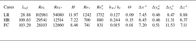
 x^ref
 Reδ=ρeUeδ/μe
 δ
 Reδ∗=ρeUeδ∗/μe
 δ∗
 H=δ∗/θ
 θ
 Reτ=ρwuτδ/μw
 Reτ∗=ρeτwδ/μe
 Θ=(hw−he)/(hr−he)
 hr=he+rue2/2
 r=0.9
 Δx+
 Δyw+
 Δye+
 Δz+
 x
 y
 y
 y=δ
 z

 Y~s
 2
 2
 M¯/Me

 u~/ue
 ρ¯/ρe
 T~/Te
 h~/he
 μ¯/μe
 ρ¯/ρe
 T~/Te
 h~/he
 h(T~,Y~s)/he

 DasLE

 CT′′Ys′′

 T′′/T~
 YO′′/Y~O
 x
 z
 y∗≈200

 h′′2~/h~2

 Prt,T
 Prt,h
 Sct,Ys

 h
 T
 Ys

 Cu′′h′′
 Cu′′ht′′
 Cu′′v′′/Cv′′h′′
 Cu′′v′′/Cv′′ht′′

 αhtu=Cu′′ht′′
 αhtu
 0.97⩽αhtu⩽1

 ln(1−αhtu)
 Θ
 ln(1−αhtu)=3.675Θ−4.473
 αhtu

 R˙¯r
 R1
 R2
 R3
 R˙T~,ρ¯s
 R˙Wi
 R˙p¯

 R˙¯r
 R4
 R5
 R˙T~,ρ¯s
 R˙Wi
 R˙p¯

 ω˙¯s
 2
 2
 ω˙sPDF
 ω˙s,p¯PDF

 ω˙¯s
 ω˙s,p¯PDF
 ω˙sPDF
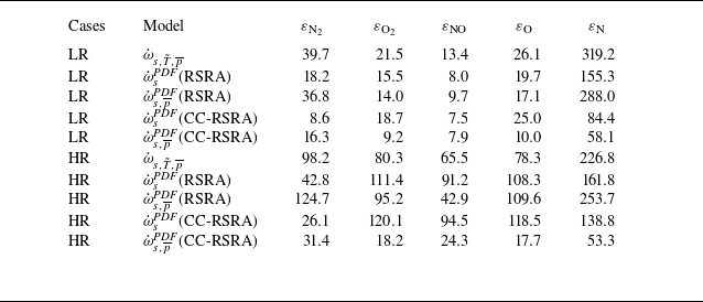
 L2

 Cf
 Cq
 Reθ
 AReθ−B
 A=0.0131
 B=0.0268

 YO

 u¯/ue
 T¯/Te
 Y¯s
 2
 2

 Ys,w

 x^ref
 Reτ=1104
 Reτ=905

 ρ¯/ρe
 T~/Te
 x^ref

 X~s
 2
 2
 x^ref
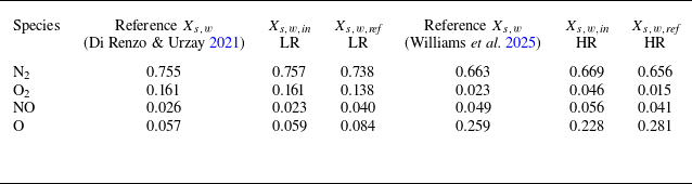
 2
 2
 Xs,w,in
 Xs,w,ref
 Reτ=1104
 Reτ=905


