

Published online by Cambridge University Press: 17 March 2006
We estimate a threshold autoregressive model to assess medieval financial integration. Our approach is based on the analysis of deviations between exchange rates and parity, which in a fully integrated market should not exceed bullion points. Hence, the time needed for adjustment, following a violation of the bullion points, is a measure of integration. We apply this approach to exchange between fourteenth- and fifteenth-century Flanders, Lübeck, and Prussia, results showing that whereas it took about eight months to reduce deviations between Flanders and Lübeck by 50 percent, those between Flanders and Prussia were roughly twice as persistent.
Market integration in preindustrial Europe is a subject that is receiving increasing attention. Most recent studies concern markets for commodities such as grain or spices and make use of the method based on the Law of One Price on commodity markets.1
Compare Persson, Grain Markets.
Our focus is on financial markets, which are a suitable benchmark for other commodities. Financial markets integrated more easily than any others, so that it seems obvious that when they were badly integrated, markets for other commodities fared even worse. Our method for analysing their integration is simple enough. In a world with commodity money and perfect monetary integration, exchange rates are pinned down by the bullion content of coins; in the case we are analyzing here, by their content of silver. In the presence of transaction and transport costs, exchange rates can fluctuate randomly around silver parity up to these costs, which in effect define silver points.2
Flandreau, “Water Seeks a Level”; Officer, Between the Dollar-Sterling Gold Points; Sergent and Velde, Big Problem; and Canjels, Prakash-Canjels, and Taylor, “Measuring Market Integration.”
Canjels, Prakash-Canjels, and Taylor (“Measuring Market Integration”) are following a related approach with regard to the late nineteenth- and early-twentieth-century gold standard period.
We chose to study the region that was dominated by the Hanseatic League in the fourteenth and fifteenth centuries. The period is particularly suitable because, at that time, fiat money still played a minor role. Bills of exhange were used but, before they became negotiable in the late sixteenth and seventeenth centuries, prices that were independent from the exchange rates of coins could hardly develop for them.4
We are well aware of the possibility that rates quoted in bills of exchange may have contained a hidden interest rate (see de Roover, Bruges Money Market pp. 32 ff.), and that this might distort our data. However, as almost all quotations that we found in bills of exchange are from the first two decades of the fifteenth century, and as we have very few other observations from that period, there is insufficient material to determine how far exchange rates of both types diverged. The full data that we used are given in Volckart and Wolf, “Estimating Medieval Market Integration” (accessible at http://www.wiwi.hu-berlin.de/wg/volckart/14_16_exchange_rates.xls). There, we indicate the type of quotation, using the categories developed by Spufford, Handbook, pp. l ff.
Spufford, Handbook, p. xxxi; and Day, “Great Bullion Famine,” p. 2.
As for the region, the main reason why we chose it was that we were able to collect a broad, new data set based on relatively homogeneous sources such as the account books of merchants and urban councils. Also, the Hanseatic area is easy to analyze because, in contrast to most of Western Europe, it was dominated by currencies based on only one precious metal, i.e., silver.6
Spufford, Money, pp. 282 f.
Compare Munro, Wool, pp. 29 f.
Stromer, “Der innovatorische Rückstand.”
Despite the overall backward character of the Hanseatic area, coins do seem to have been shipped speculatively. Merchants did not make a fundamental distinction between them and other commodities, calling exchange transactions the “purchase” and “sale” of coins. In a similar vein, the use of bills of exchange was called “overkof,” which can be translated as “sale at a distance.”9
See for example Mollwo, Handlungsbuch, pp. 30, 33; and Lesnikow, Handelsbücher, p. 39.
In this section, we discuss three currencies: the Flemish pound grote and the marks of Lübeck and Prussia. The pound grote was issued by the counts of Flanders and later by the dukes of Burgundy.10
Spufford, Monetary Problems; and Munro, Wool.
Jesse, Der Wendische Münzverein; and Stefke, “Der ‘Wendische Münzverein.’”
Volckart, Münzpolitik.
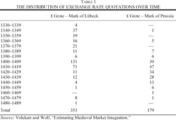
As a rule, the quality of medieval data leaves much to be desired, and the exchange rates of our currencies, though being better preserved than most other data from this period and region, are no exception. One problem is their uneven distribution over time. As shown by the following table, some decades are covered densely, whereas for others data are scarce or entirely lacking (see Table 1).
However, restricting our attention to periods for which data are plentiful—that is, for Flanders-Lübeck to 1340 to 1440, and for Flanders-Prussia to 1380 to 1450—eliminates much of the problem. For these periods, so many data exist that few interpolations are needed. In fact, for Flanders-Lübeck during the period 1403 to 1423 we can even construct a series of quarterly data, which allows an in-depth analysis. It is an additional advantage that most of the quotations from this period stem from a single group of closely related sources, i.e., from the account books and commercial correspondence of the Hanseatic merchant Hildebrand Veckinghusen.13
Stieda, “Ein Geldgeschäft,” Hansisch-venetianische Handelsbeziehungen, and, Hildebrand Veckinghusen; and Lesnikov, Handelsbücher.
Most of the rest of the quotations are from other contemporary account books, see for example Koppmann, Kämmereirechnungen, and Sattler, Handelsrechnungen. For the full references see Volckart and Wolf, “Estimating Medieval Market Integration.”
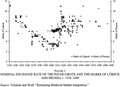
We should stress here that we use market rates only, that is, rates that developed under the impact of supply and demand. Occasionally, political authorities imposed exchange rates that obviously differed from those paid on financial markets (that was the point of imposing them); using them would distort our results. Moreover, such rates applied to exchanges that took place at the mint where people had to pay charges and seignorage taxes when they wanted to exchange their money. Such costs figure as additional transaction costs; they are a further source of distortions, which we want to avoid. Keeping these points in mind, curves of the nominal exchange rates of the pound grote in marks of Lübeck and marks of Prussia in the time we are discussing can be constructed (see Figure 1).
FIGURE 1 NOMINAL EXCHANGE RATE OF THE POUND GROTE AND THE MARKS OF LÜBECK AND PRUSSIA
Apart from the exchange rates, we base our analysis on the silver equivalents of the pound grote and the marks of Lübeck and Prussia. Here, too, some explanations are in order, notably because Raymond de Roover was openly sceptical of attempts to link the bullion content of medieval coins with their exchange rate, claiming that monetary ordinances give no idea of the actual state of the currency at a given time.15
De Roover, Bruges Money Market, p. 38.
Volckart, Münzpolitik, p. 194.
Ropp, Hanserecesse, vol. 4, p. 209.
As for the silver content, the data for Flanders are given in van Werveke, “De economische en sociale gevolgen,” p. 244; Munro, Wool, p. 211; and Blockmans and Blockmans, “Devaluation,” pp. 83, 89. The data for the Wendish Union are from Jesse, Der Wendische Münzverein, pp. 209 ff.; and those for Prussia from Volckart, Münzpolitik, p. 435.
However, over time coins became worn down, losing some of their weight and precious metal. This problem has been extensively discussed in the literature, but in our context it is not as serious as it seems to be at first glance.19
Compare Mayhew, Numismatic Evidence, p. 3; and North, Geldumlauf, p. 108.
Munro, “Bullion Flows,” p. 136; Jesse, Der Wendische Münzverein, pp. 238 ff.; and Volckart, Münzpolitik, p. 91.
Apart from monetary ordinances there are other sources that contain information about the coins' content of specie. Occasionally, contemporary political authorities assayed the money in circulation, and, increasingly, medieval coins are being chemically analyzed in the context of modern research.21
See for example Kubiak, Monety.
Volckart, Münzpolitik, p. 91.
Ropp, Hanserecesse, vol. 2, p. 225.
FIGURE 2 SILVER EQUIVALENTS OF THE POUND GROTE AND THE MARKS OF LÜBECK AND PRUSSIA, C. 1320–1490
The Prussian case gives evidence of another problem posed by changes in the standard of the coinage: Whereas after a debasement it was in everybody's interest as quickly as possible to exchange his old coins for a larger nominal sum of new ones, after a re-enforcement of the coinage the old money tended to continue to circulate. No one was interested in taking it to the mint where he would receive not even the silver-equivalent (the costs of re-minting and seigniorage taxes having been deduced), but an even smaller nominal sum. Prussia, which between the re-enforcement of 1416 and the debasement of 1454 practically had two parallel currencies—the old or “lesser” and the new or “good” mark whose official ratio was 2:1—is an extreme case, but similar problems occurred in Flanders, too.24
Volckart, Münzpolitik, pp. 97 f.; for an example of the parallel circulation of old and new money in Flanders see Sattler, Handelsrechnungen, p. 517.
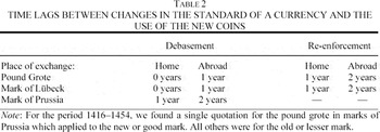
A final factor, which should be taken into account, is the distance of the exchange transaction to the place of origin of the coins involved. It seems reasonable to assume that abroad, older coins continued to circulate some time after they had been replaced by new ones at home. Hence, we need to make a distinction between several factors when we want to determine the delay between the official change in the standard of coinage and the time when the new coins dominated circulation: the direction of the change of standard (debasement or re-enforcement), the administrative abilities of the authority that issued the currency (relatively good in Flanders and in the Wendish cities, bad in Prussia), and whether the coins were exchanged at the place where they had been minted or abroad. In calculating the exchange rate that would have corresponded to silver parity, we consequently need to take a time-lag into account. Table 2 lists our assumptions.
In this section we estimate the degree to which money markets between Flanders, Lübeck, and Prussia were integrated. The challenge to estimating integration is to account for the nonlinearity of the adjustment process. Arbitrage between locations will only take place if expected gains are sufficiently high to cover the costs of information, insurance, and shipment, which define the silver points. We consequently expect that the behavior of nominal exchange rates at which coins were traded between Flanders, Lübeck, and Prussia will show a regime switch once exchange rates deviate far enough from the underlying rate of their silver contents. For exchange rate deviations within the silver points, the nominal rate should behave like a stationary disturbance term. By contrast, for deviations outside the points, we expect a nonstationary behavior of the series, i.e., an adjustment process back towards the underlying rate of silver contents. As shown by Maurice Obstfeld and Alan M. Taylor, the appropriate framework for modeling such a process is that of a threshold autoregression (TAR) model.
25Obstfeld and Taylor, “Nonlinear Aspects”; and Taylor, “Potential Pitfalls.”
Volckart and Wolf, “Estimating Medieval Market Integration”; see also Canjels, Prakash-Canjels, and Taylor, “Measuring Market Integration.”


We expect the behavior of exchange rates to be driven by deviations from parity relative to the costs of arbitrage. Specifically, we estimate

where α, β, and τ are parameters to be estimated. The parameter τ captures the effect of arbitrage costs expressed per silver unit. When arbitrage in the money market is unprofitable, the deviation between the observed exchange rate and silver parity behaves like a stationary disturbance term, υt. The key prediction of the model is that if the exchange rate exceeds silver parity by more than the limit set by τ, arbitrage in silver will force it to revert to within those limits. The speed of that adjustment process is estimated by the coefficient α. When derived from a structural model, it can be shown that this speed of adjustment depends on the structural elements of the economy such as costs of seignorage and on nonlinear parts of the arbitrage costs due to possible risk-aversion of traders.
27Volckart and Wolf, “Estimating Medieval Market Integration.”
Because our task of estimating a nonlinear TAR model is rather demanding in terms of the quality of the data, we will focus on the years between 1385 and 1450 for which they are most complete and available for both Flanders-Lübeck and Flanders-Prussia. Moreover, we also estimate the model based on quarterly data, which is available for Flanders-Lübeck in the period 1403 to 1423. As a general rule, we always convert our observations into a continous series of data points where we use simple averages for periods with more than one observation and interpolation techniques to deal with missing data. In order to account for the fact that we have more information for some years than for others, we weight the resulting annual (or quarterly) time series by the number of observations for each year (or quarter).
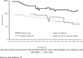
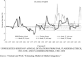
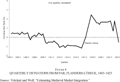
Before we proceed to the estimation of our model, we will first check whether Xt, the unweighted annual series of exchange rate deviations from par, is a stationary process or whether it contains a unit root. With a unit root, we would expect to see some trending behavior over the whole period, which would be incompatible with the basic implication of our model that large deviations from par should trigger an adjustment process due to arbitrage in silver. Figure 3 plots the annual series of Xt over time, and Figure 4 plots the quarterely data for the early fifteenth century.
FIGURE 3 UNWEIGHTED SERIES OF ANNUAL DEVIATIONS FROM PAR, FLANDERS-LÜBECK, 1341–1450, AND FLANDERS-PRUSSIA, 1385–1454
FIGURE 4 QUARTERLY DEVIATIONS FROM PAR, FLANDERS-LÜBECK, 1403–1423
The annual series do indeed give a realistic picture of exchange rate dynamics insofar as there is little evidence of higher frequency adjustment processes that would be undetectable from annual averages.
28See Taylor, “Potential Pitfalls.”
Volckart, Münzpolitik, pp. 35, 49; compare Bernholz, “Bedeutung der Geschichte,” pp. 144 f. There is quite a lot of anecdotal evidence for shipments of silver from Prussia to the West: Stieda, Hildebrand Veckinghusen, pp. 183 f., 186 f., 198 f., 201 ff., 255 f. However, we did not find any evidence for shipments from Flanders or Lübeck toward Prussia.
Both an Augmented Dickey-Fuller and a Phillips-Perron test clearly reject the null-hypothesis of a unit root: for Flanders-Lübeck annual: ADF statistic: –3.21, McKinnon value (1 percent): –2.58, PP statistic: –3.21, McKinnon critical value (1 percent): –2.58. For Flanders-Prussia annual: ADF statistic: –2.82, McKinnon value (1 percent): –2.60, PP statistic: –2.76, McKinnon critical value (1 percent): –2.60. For Flanders-Lübeck quarterly: ADF statistic: –1.690, McKinnon value (1 percent): –1.614, PP statistic: –1.655, McKinnon critical value (10 percent): –1.614.
Canjels, Prakash-Canjels and Taylor, “Measuring Market Integration.”

where indicator is a variable that takes on the value of one if we are outside the intermediate random-walk regime, and has no value otherwise, while Pos and Neg indicate silver export and import regimes. The parameters C1, C2, and C3 are equivalent to the model parameters α, τ, and β respectively. According to our model, and as usual in TAR models, the points of regime switch are identified by the fact that within these points the series should behave like a (nonstationary) random walk.
32See Balke and Fomby, “Threshold Cointegration”; and Lo and Zivot, “Threshold Cointegration.”

+ εt. The estimated series of errors from that series can be used to create an indicator variable for regime switch: large (positive or negative) deviations indicate that the series cannot be represented any more by a random-walk regime, suggesting that one of the other two regimes applies.
33Here we define an error larger than the median of absolute errors as “large.” We experimented with several other specifications with only very small effects on our results.
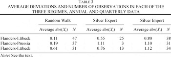
In all three cases, about half of the observations are estimated to be outside the random-walk regime. As expected, we see that the average of absolute deviations under a random-walk regime is lower than under the other two regimes. Overall, we expect to find that changes in deviations ΔXt are declining in previous deviations Xt−1, hence −1 < C1 < 0, and we expect to find some positive threshold level C2 > 0. Finally, we expect to find C3 < 0 as implied by our economic model. The next section contains the results of that exercise and our interpretation.
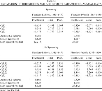
Our procedure to estimate the points of regime switch delivered quite reasonable results, so that we estimate our model as described in equation 3. We first assume symmetry across regimes; next we relax this to allow for regime-specific coefficients (see Table 4).
Most of the estimated coefficients are significant at a 5 percent level, and, as predicted, we always find a negative adjustment parameter C1 and a positive threshold C2, which seems of reasonable magnitude given the average deviations under the random-walk regimes in both our cases. Also, the coefficient on parity changes has the expected negative sign. Next, we repeat the estimation without the assumption of symmetry between the silver import and silver export regimes. In the case of Flanders-Prussia in particular, Figure 3 suggests some significant differences. Two findings stand out. First, the statistical significance of the adjustment coefficients is much lower, which is no surprise given the small number of observations under some of the regimes. Second, given lower significance, the estimated adjustment under a silver import regime in the case of Flanders-Lübeck does not appear to have taken place much faster than in the case of Flanders-Prussia. However, the estimated threshold levels for Flanders-Lübeck are still much lower, indicating that adjustment set in earlier.
How shall we interpret these findings? As expected, the money market between Flanders and Lübeck was much better integrated than the market between Flanders and remote Prussia. The estimate C2 for transport and information costs (τ in the economic model) is much higher for the latter case. And the estimates C1 indicate a significantly higher speed of adjustment between Flanders and Lübeck than between Flanders and Prussia. In order to interpret the estimated adjustment parameters, it is useful to express them in terms of a half-life time. We rearrange equation 2 to get

Hence, the implied half-life can be calculated as

. Our estimates imply that between 1385 and 1450, it took on average about eight months until arbitrage in silver reduced a deviation outside the threshold bands between Lübeck and Flanders by 50 percent. During the same period it took on average about 21 months to reduce a deviation between Prussia and Flanders.
Finally, all these estimates suffer from the fact that we use annual data, which implies that adjustment processes with a half-life of less than six months cannot possibly be identified.34
Compare Taylor, “Potential Pitfalls.”
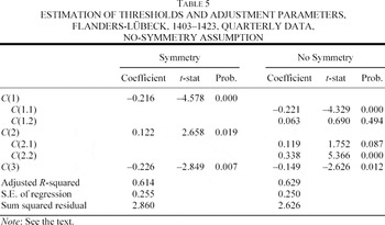
The fit of the model has improved, and for the symmetric case all coefficients are statistically significant at the 5 percent level. Without the assumption of symmetry, only the adjustment coefficient under a silver import regime is estimated to be statistically different from zero. Interestingly, both that coefficient and the coefficient under the symmetry assumption imply a half-life of

quarters, that is, of about eight months. This is perfectly in line with our estimate based on the annual series and again indicates that higher-frequency adjustment was—at least during the period 1403–1423—not taking place. Given this, our estimated half-lifes of between eight and 21 months based on annual data can be compared with those implied by Canjels et al.'s estimation for the Gold Standard period.
35Canjels, Prakash-Canjels, and Taylor, “Measuring Market Integration.”
Canjels, Prakash-Canjels, and Taylor, “Measuring Market Integration.”
Financial markets integrate more easily than those for other goods. In the context of research done on medieval market integration, it therefore makes sense to pay special attention to them: they can be used as a benchmark for other markets that arguably could not be better-integrated than they. In this article, we study late medieval financial integration not only on the basis of a new data-set that comprises exchange rates from a hitherto neglected area, but also with the help of the recently developed TAR-modelling approach.37
Spufford's “Handbook of Medieval Exchange” contains few data from the Hanseatic area.
Compare Canjels, Prakash-Canjels, and Taylor, “Measuring Market Integration.”
We presented an earlier draft of this article at the “Berlin Coloquium – A Workshop in Quantitative Economic History” in September 2004, and would like to thank participants for their advice and suggestions. Also, thanks are due to the three anonymous referees who made a large number of valuable suggestions.
TABLE 1 THE DISTRIBUTION OF EXCHANGE RATE QUOTATIONS OVER TIME

FIGURE 1 NOMINAL EXCHANGE RATE OF THE POUND GROTE AND THE MARKS OF LÜBECK AND PRUSSIA

FIGURE 2 SILVER EQUIVALENTS OF THE POUND GROTE AND THE MARKS OF LÜBECK AND PRUSSIA, C. 1320–1490
TABLE 2 TIME LAGS BETWEEN CHANGES IN THE STANDARD OF A CURRENCY AND THE USE OF THE NEW COINS

FIGURE 3 UNWEIGHTED SERIES OF ANNUAL DEVIATIONS FROM PAR, FLANDERS-LÜBECK, 1341–1450, AND FLANDERS-PRUSSIA, 1385–1454

FIGURE 4 QUARTERLY DEVIATIONS FROM PAR, FLANDERS-LÜBECK, 1403–1423
TABLE 3 AVERAGE DEVIATIONS AND NUMBER OF OBSERVATIONS IN EACH OF THE THREE REGIMES, ANNUAL AND QUARTERLY DATA
TABLE 4 ESTIMATION OF THRESHOLDS AND ADJUSTMENT PARAMETERS, ANNUAL DATA
TABLE 5 ESTIMATION OF THRESHOLDS AND ADJUSTMENT PARAMETERS, FLANDERS-LÜBECK, 1403–1423, QUARTERLY DATA, NO-SYMMETRY ASSUMPTION