

The incumbency advantage is an important phenomenon in US politics, but even after years of study it is not clear what it represents. One possibility is that it mainly captures a scare-off effect. The logic is straightforward. If “high quality” challengers are especially strategic in their behavior, and wait for open seats to become available rather than challenge incumbents, then most incumbents will face “low quality” challengers (or no challenger at all). It is therefore possible that incumbents do well in their re-election attempts not because they are particularly high quality or enjoy large officeholder benefits, but simply because their opponents are low quality.
This argument is made forcefully in Cox and Katz (Reference Cox and Katz1996) and Levitt and Wolfram (Reference Levitt and Wolfram1997). Cox and Katz (Reference Cox and Katz1996) write, “Most of the increase in the incumbency advantage, at least down to 1980, came through increases in the quality effect (i.e., the advantage to the incumbent party of having a low-quality challenger)” (p. 478). Levitt and Wolfram (Reference Levitt and Wolfram1997) reach a similar conclusion, arguing that “a large fraction of the incumbency advantage is the result of incumbents’ apparent ability to deter high-quality challengers. Virtually all of the growth in the incumbency advantage since the 1960s appears to be attributable to a reduction in the relative quality of challengers” (p. 56).
The idea that a large part of the incumbency advantage is due to scare-off may have reached the status of conventional wisdom. For example, in his widely used text The Politics of Congressional Elections, (Jacobson Reference Jacobson2009, 42) writes: “The electoral value of incumbency lies not only in what it provides to the incumbent but also in how it affects the thinking of potential opponents and their potential supporters. Many incumbents win easily by wide margins because they face inexperienced, sometimes reluctant, challengers who lack the financial and organizational backing to mount a serious campaign for congress.” In the Encyclopedia of Campaigns, Elections and Electoral Behavior, Sidman (Reference Sidman2008) writes: “High quality challengers often do not want to waste the resources they have built in an unsuccessful challenge. Before emerging, they will look at a variety of factors that signal how vulnerable the incumbent is and weigh the likelihood of winning office. Given the strength of many incumbents, it takes the right mix of incumbent vulnerability and national political climate … for a high-quality challenger to emerge” (p. 118). Finally, in Conventional Wisdom and American Elections, Baumgartner and Francia (Reference Baumgartner and Francia2010) write: “Experienced politicians or prominent leaders have enough political savvy to know that the chances of beating an incumbent are slim. Generally, only open-seat races attract quality candidates … This is the so-called scare-off effect, and while it is clear that anything can happen in a campaign, most challengers are amateurs who pose little threat to incumbents” (p. 151).
As the last quote suggests, the argument is particularly plausible in light of the fact that one of the best measures of candidate quality is previous officeholder experience. Intuitively, many of the strongest candidates are elected officials who hold offices similar to those they are seeking and with similar constituencies—for example, state legislators running for the US House, state representatives running for the state senate, or state attorneys general running for governor. Strategic entry by such high-quality challengers can then be explained as the result of the opportunity costs that officeholders face. Current officeholders have a high opportunity cost of running for higher office, since they typically must give up their current office. This leads them to wait for an incumbent to retire, and to disproportionately enter races where their party is favored. Several theoretical papers formalize the scare-off effect.Footnote 1 In addition, previous empirical work finds strong evidence of strategic challenger behavior.Footnote 2
In this paper we provide a causal estimate of the impact of incumbency on candidate officeholder experience in the opposition party, using a regression discontinuity (RD) design. More specifically, we exploit the “as-if random” assignment of incumbency status to the winner in very close elections, and thereby isolate the effect of party incumbency status on the experience of each party’s candidate in the next election.Footnote 3 , Footnote 4 We follow previous work and measure quality in terms of prior officeholder experience. Jacobson (Reference Jacobson1989, Reference Jacobson2009), Squire (Reference Squire1992), Cox and Katz (Reference Cox and Katz2002), Carson et al. (Reference Carson, Engstrom and Roberts2007), and many others find that candidates who previously held elective office have significantly larger vote shares and significantly higher probabilities of winning than other candidates.Footnote 5 We study US House elections, state legislative elections, and elections for statewide offices, including the US Senate.
The bottom line is easily stated: we find a very small scare-off effect. Summary statistics reveal that, when a party loses a close election, the probability that it fields an experienced challenger in the next election cycle falls by only 0.3 percentage points in the US House, and by only 4 to 12 percentage points in statewide and state senate elections. Using the more rigorous RD estimator, we again find small estimates for the effect of party incumbency on the subsequent experience gap between the incumbent and challenger in the next election, and we cannot reject the null hypothesis that incumbency has no effect on this differential.
Finding a small scare-off effect when the incumbent party won by a very close margin in the previous race would be relatively uninteresting if there were little or no party incumbency advantage in these cases. However, as many previous papers have shown (and as we confirm below for our samples), the party incumbency advantage in these cases is quite large. In fact, it is about as large as the estimates of the incumbency advantage based on other methods that use all available races. For example, Fowler and Hall (Reference Fowler and Hall2015) use the Lee (Reference Lee2008) RD strategy in state legislatures and estimate that incumbency causes an overall increase of 7.8 percentage points in vote share. Using the same data, Fowler and Hall (Reference Fowler and Hall2015) estimate that the “sophomore surge” estimate (Erikson Reference Erikson1971) of the incumbency advantage, which uses almost all elections, is 4.7 percentage points—if anything, smaller than the incumbency advantage when estimated using only close elections.Footnote 6
Combining our results with estimates from the literature about the effect of candidate officeholder experience on the probability of winning elections (and vote share), we can estimate how much of the party incumbency advantage appears to be due to scare-off. We calculate that scare-off can account for only 5–7 percent of the incumbency advantage across the House, statewide offices, and state senates. Even if we use a “high” hypothetical estimate of the return to experience, we still find that scare-off only explains 10–15 percent of the incumbency advantage. We also investigate whether there is more scare-off in the long-term—two or more elections downstream—but find no significant long-term scare-off.
How do we interpret our findings? First, the RD analysis gives a local estimate of the effect of winning in close races.Footnote 7 It is therefore possible that in cases where the previous election was not close the incumbency advantage is mainly due to scare-off. However, it is not obvious that incumbency status itself should cause more scare-off in safer districts. The fact that incumbents tend to face fewer experienced challengers in safe districts does not, by itself, imply that the scare-off effect due to incumbency is larger in safe districts. For example, consider the calculus of an experienced Republican candidate in a safely Democratic district. She might be reluctant to run simply because the normal vote is against her. In order to assert that scare-off is larger in the safe district, we would have to show that the decrease in the probability that she would run caused by the presence of a Democratic incumbent (compared to an open-seat election) in this safe district is larger than the analogous decrease in the more competitive district. It is not obvious that this differential ought to be larger in safe districts, and for now we remain agnostic.
Second, we are not arguing that experienced challengers are not strategic. On the other hand, they are not perfectly strategic, or perfectly foresighted, either. The R 2 statistics in the literature from regressions predicting candidate experience are far from 1, indicating that idiosyncratic factors lead some experienced candidates to run while others stay out. These factors might be term limits, dissatisfaction with the current office held, decisions to “move up or move out” of politics as a career, staggered terms (e.g., state senators with four-year terms or local officials elected in odd-numbered years who can challenge incumbents without giving up their current offices), and so on.
Regardless, the set of districts in which close races are likely to occur—mainly marginal districts in which the distribution of partisan affiliations of voters is relatively balanced—is especially relevant for key questions regarding the US electoral system. Does the incumbency advantage lead to persistence in the identity of the majority party, as well as to dampened responsiveness to shifts in voter preferences? If so, is this mainly due to the ability of incumbents to scare-off experienced candidates in the marginal districts that are most likely to flip between parties? Is it the case that even in marginal districts—where an underperforming incumbent would be especially vulnerable to a strong challenge from the other party—incumbents remain in office mainly due to their ability to scare-off experienced opponents? Our findings suggest the answers to the second question and third questions are: “probably not.”
Data and Specifications
The US House elections data are from Dubin (Reference Dubin1998) and the Office of the Clerk of the US House of Representatives.Footnote 8 The statewide office elections data are from official state sources.Footnote 9 The state legislative elections data are from ICPSR Study #34297. The data on candidate previous experience for US House candidates was graciously provided by Gary Jacobson, and supplemented by the electoral data itself (tracking previous winners), along with various issues of Congressional Quarterly Weekly Reports. The data on candidate previous experience for statewide races and state senates is from the electoral data.
We follow the previous literature in the exact definitions of which previous offices count for the quality indicator, which is a binary variable taking on the value 1 if the candidate has held one of these offices in the past, and 0 otherwise. Candidates running for the US House are considered to be of quality if they hold, or have previously held, any of the following offices: state representative, state senator, any statewide office, US Senate, another US House seat, or a local office (including mayor, city council, county commissioner, district attorney, etc.). Candidates running for statewide office are considered to be of quality if they hold, or have previously held, any of the following offices: state representative, state senator, any statewide office, US Senate, US House, or mayor. Finally, candidates running for state senate are considered to be of quality if they hold, or have previously held, any of the following offices: state representative or another state senate seat.
We employ a standard RD design. The forcing variable is the Democratic share of the two-party vote, Democ Vote Pct, and the threshold separating winners from losers is 50 percent.Footnote 10 Thus, our specification is
 $$Y_{{i,\,t{\plus}1}} =\beta \;Democ\;Win_{{it}} {\plus}f(Democ\;Vote\;Pct_{{it}} ){\plus}\epsilon _{{it}} ,$$
where f is either a local linear or polynomial control function and Y is the dependent variable of interest.Footnote 11 We estimate this equation using a small bandwidth around the discontinuity. In the body of the paper, all results are presented using a 5 percent bandwidth, that is, using all elections in which the winning candidate obtained 50–55 percent of the two-party vote.
The parameter of interest is β, which provides an estimate of the causal effect of winning at time t on Y at t+1. The dependent variables are: Democ Win, Democ Vote, Pct, Democ Cand Experienced, Repub Cand Experienced, and Net Cand Experience≡Democ Cand Experienced—Repub Cand Experienced. We use the first two dependent variables to estimate the party incumbency advantage. We use the last three dependent variables—particularly the last variable—to estimate scare-off.Footnote 12 Importantly, in constructing these variables we do not include the experience due to incumbency that is “automatically” acquired by the party that wins at time t, in the event that party’s candidate runs again at time t+1.Footnote 13 Thus, for the last dependent variable, β provides an estimate of the causal effect of winning at time t on the difference in candidate experience between the parties at time t+1 (other than that acquired via incumbency due to the outcome at time t). If this is large and negative then it indicates a large amount of scare-off.
Following best practices, in the Appendix we show that our results are robust to the use of a wide variety of bandwidth sizes and specifications of the forcing variable. In addition, it is important with any design to test the validity of the identifying assumption wherever possible. In the RD framework, this is done by checking for evidence of sorting around the discontinuity at time t. Fortunately for the present study, Eggers et al. (ND) studies the same elections used in this paper (along with others), and finds no evidence of sorting. In addition, in the Appendix we present further evidence that the districts with close Democratic winners and those with close Republican winners exhibit no differences in net experience differential at time t—further validation of the RD assumption. As a result, there is no evidence that sorting is an issue for the analysis.
Results
Summary Measures
We begin with some summary statistics, which are in the spirit of “naive” RD estimates. Consider the following questions: After winning a close election at time t, what is the probability that a party goes on to win at time t+1? What is the probability that the opposing party runs an experienced candidate at time t+1, and how does this compare to the probability that the opposing party ran an experienced candidate at time t? What is the probability that the winning party runs an experienced candidate at time t+1, not counting the experience “automatically” accumulated by the victory at time t? How does this compare to the probability that the party ran an experienced candidate at time t?
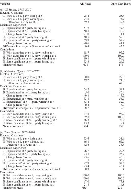
Table 1 shows these statistics for US House races, statewide office races, and state senate races. In this table we first consider all cases where the race at time t was close, and then focus on cases where the election at time t was an open-seat race (and close). In all cases we define a race as close if the winner received between 50 and 52 percent of the vote.Footnote 14
Summary Statistics on Candidate Experience and Winning (Win Margin <2)

a The officeholding due to the victory at t is not included in calculating % experienced for the party winning at t.
Consider Table 1a. The top panel shows that the incumbent party in a district wins much more often than 50 percent of the time. More specifically, the difference in the probability of winning at time t+1 between the winning and losing parties at time t is about 49.3 percent (row 3 of the table). Not surprisingly, this is similar to the RD estimates in Lee (Reference Lee2008).
Next, consider the middle panel. The first row of this panel shows the percentage of cases in which the party losing the election at time t fields an experienced candidate at time t. The second row shows the percentage of cases in which this party fields an experienced candidate at time t+1. The difference between these two rows gives a crude estimate of the scare-off effect, which, if it is present, should produce a negative change in the probability of an experienced candidate for the losing party. Thus, for example, in the first column (all races) we see that the percentage falls from 51.2 to 50.1 percent, suggesting an initial scare-off estimate of 1.0 percentage points. In the second column (open-seat races) we see that the percentage actually increases from 47.8 to 48.9 percent, the opposite of what we would expect from scare-off.
The fourth row of this panel shows the percentage of cases in which the party winning the election at time t fields an experienced candidate at time t. The fifth row shows the percentage of cases in which this party fields an experienced candidate at time t+1. As noted above, this row does not include the “automatic” experience acquired due to the victory at time t, in the event that the candidate winning at time t runs again at time t+1.Footnote 15 The difference between these two rows shows that the percentage of experienced candidates even falls a bit in the party that wins at time t, likely due to occasional retirements.
Row 10 of the table shows the difference between rows 9 and 6 of the table. This gives a more complete measure of the “differential change in quality” between the time t winning and losing parties (again, not including the experience acquired due to the victory at time t). If scare-off is present, we would expect the change in experience for the winning party to be less negative than the change for the losing party—and thus to see a positive difference. We see that these figures are 0.4 percent for all races, and −2.2 percent for open-seat races. That is to say, there is very little difference in the change in experience across the winning and losing parties, and this change is not consistent in sign across open-seat races and all races. This does not suggest a large scare-off effect.
The final panel looks at one possible mechanism for the small scare-off effect. Perhaps losing candidates often run again the next time, undeterred by their previous defeat and by their opponent’s new incumbency status. The summary statistics suggest that, while losers do sometimes run again (33.3 percent of the time), they comprise only a small part of all challenger candidates at t+1. The party losing at t fields a candidate in 98.7 percent of all races at t+1; repeat-challengers thus comprise only roughly a third of the pairings at t+1. Another possible implication of this hypothesis—a theory of “sticky” challenger decisions—is that the scare-off effect should grow as time passes since the assignment of incumbency at time t. Later in the paper we test this related hypothesis and find no evidence for it. We find no evidence for the scare-off of experienced challengers either in the short or long term.
Tables 1b and 1c show the same statistics as Table 1a, but for statewide office and state senate elections, respectively. The overall patterns in these tables are similar to those in Table 1a. First, there appears to be a large party incumbency advantage—the difference in the probability of winning at time t+1 between the winning and losing parties at time t is around 40 percent. Second, there appears to be relatively little scare-off—the differential change in experience between winning and losing parties at time t is around 8–10 percent for statewide offices and <1 percent for state senate districts. Like the results for the US House, it is unlikely that scare-off causes a significant part of the (large) party incumbency advantage in these other offices.
RD Estimates
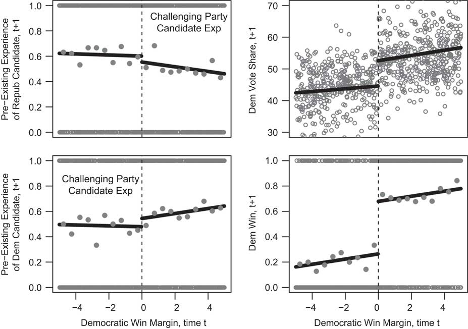
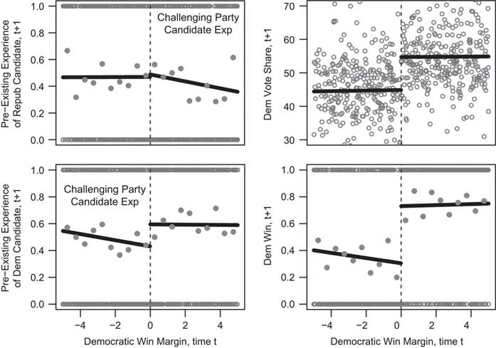
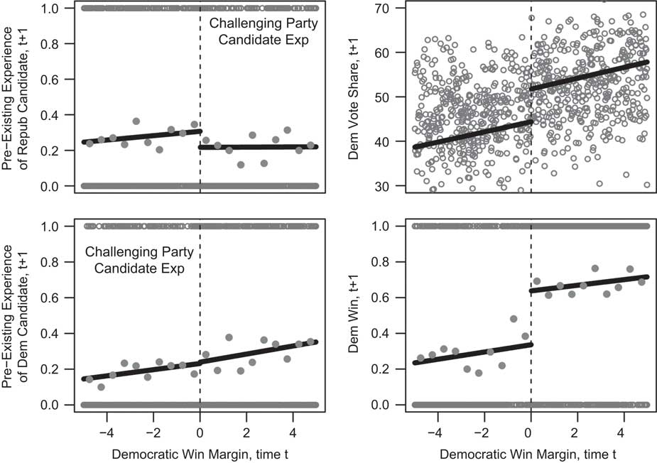
We now turn to a more rigorous RD analysis. Following convention, we begin by presenting graphical versions of the analyses for all three contexts. Figures 1, 2, and 3 present the data for the US House, statewide offices, and state senates, respectively. Each figure contains four panels. In the first column, the plots show the change in candidate experience for each party, respectively, as the Democratic party goes from barely losing to barely winning elections. There is almost no discernible “jump” in these graphs, suggesting that there is little scare-off in these close elections. In contrast, the second column presents the results of these same close Democratic wins and losses on subsequent Democratic vote share (top row) and victory (bottom row). Here, large discontinuities are present.
The effect of incumbency on challenger experience and incumbent party vote share, US House Notes: In the left column, we see little or no “jump” in subsequent candidate experience for each party when the Democratic party switches from barely losing to barely winning the election. In the right column, we see that there is nonetheless a large jump in the electoral fortunes of the Democratic party when they switch from barely losing to barely winning. Lines are from OLS estimated separately on each side of the discontinuity with binned averages overlaid for binary outcome variables.

The effect of incumbency on challenger experience and incumbent party vote share, statewide offices Notes: In the left column, we see little or no “jump” in subsequent candidate experience for each party when the Democratic party switches from barely losing to barely winning the election. In the right column, we see that there is nonetheless a large jump in the electoral fortunes of the Democratic party when they switch from barely losing to barely winning. Lines are from OLS estimated separately on each side of the discontinuity with binned averages overlaid for binary outcome variables.

The Effect of Incumbency on Challenger Experience and Incumbent Party Vote Share, State Legislatures Notes: In the left column, we see little or no “jump” in subsequent candidate experience for each party when the Democratic party switches from barely losing to barely winning the election. In the right column, we see that there is nonetheless a large jump in the electoral fortunes of the Democratic party when they switch from barely losing to barely winning. Lines are from OLS estimated separately on each side of the discontinuity with binned averages overlaid for binary outcome variables.

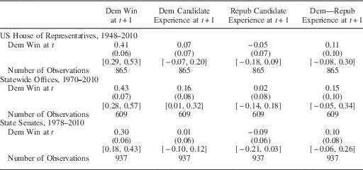
Table 2 shows the estimates for a ±5 percent bandwidth (winner received between 50 and 55 percent of the vote) and a local-linear control function. The top panel covers the US House, the middle panel covers statewide offices, and the bottom panel covers state senate seats. The columns treat different dependent variables, all based on Equation (1). The quantity of interest is the coefficient on Dem Win at t, representing the effect of a close Democratic win at time t on subsequent outcomes at time t+1. The first column estimates the party incumbency advantage. The second and third columns show effects on the probability of fielding an experienced candidate in each party at time t+1. If scare-off is present, then we should expect the effect of a Democratic win on the probability of an experienced Democratic candidate in the subsequent election to be positive in column 2, while the effect on the probability of a Republican candidate in the subsequent election should be negative in column 3. The last column shows the estimate of the effect of winning or losing at time t on the difference in candidate experience at time t+1. Like in the summary tables, we would expect the effect on this difference to be positive if scare-off is present.Footnote 16 In addition to the point estimates, we show the standard errors in parentheses and the 95 percent confidence intervals in square brackets.
Regression Discontinuity Designs Estimates, Candidate Experience, and Winning

The officeholding due to victory at t is not included in calculating experience at t+1. Robust standard errors in parentheses; 95 percent confidence intervals in brackets. Regression discontinuity designs estimates are from Equation (1), using a local linear specification of the running variable with a 5 percentage-point bandwidth.
The estimated party incumbency advantages in column 1 are all large, ranging from 30 to 43 percent—this is not surprising, of course, since they simply confirm the earlier estimates by Lee (Reference Lee2008), Fowler and Hall (Reference Fowler and Hall2015), and others for our samples.
More interestingly, none of the point estimates in columns 2–4 are substantively large. Nor are any of the point estimates in the final column statistically significant at the usual 0.05 level, or even the 0.10 level. Thus, while all of the point estimates have the sign we would expect if scare-off is operating (e.g., if the Democratic candidate wins at time t, then the Republican candidate at time t+1 is less likely to be experienced), we cannot reject the null hypothesis that the scare-off effect is zero.
Incumbency Advantage Not Explained by Scare-off
In this section we consider how much of the incumbency advantage that we observe in our samples could be explained by the scare-off effects we have estimated. We employ the following logic. Net candidate quality offers some amount of vote share to advantaged parties. If we knew the exact return to previous officeholder experience—our measure of quality—in terms of vote share, then we could evaluate how much vote share incumbents plausibly capture by avoiding quality challengers. That is to say, given our estimates of how much incumbency increases a party’s likelihood of possessing an experienced candidate and decreases the likelihood that the opponent party has an experienced candidate, we could translate this effect into vote share.
Specifically, call δ
NQD the effect of incumbency on net candidate quality in the next
election cycle, and call δ
WD the effect of incumbency on the party’s probability of winning
the next election (i.e., the overall incumbency advantage estimated in the RD).
Given a return to net candidate quality on win probability, A,
the increase in win probability due to incumbency is A δ
ZQD. In words, we multiply the increase in the candidate quality
advantage the party enjoys due to incumbency by the the rate at which this
quality advantage increases the party’s electoral prospects, so that we can
measure how much the increased quality advantage increases the party’s
probability of winning the seat. Finally, the share of the
incumbency advantage explained by this scare-off effect is thus
 $${{A \cdot \delta _{{NQD}} } \over {\delta _{{WD}} }}$$
.
Doing the calculations in this way—using a given return to net candidate quality rather than estimating it in our sample—allows us to circumvent some of the thorny issues involved in “causal mediation” analysis.Footnote 17 This problem is often of the following form. We observe causal effects of the treatment on an outcome of interest (subsequent party vote share, in our case) and on a mediating variable of interest (net candidate quality in the next election, in our case), and we want to estimate an effect of the mediating variable on the outcome so that we can parse out the two effects—that part which can be attributed to the change caused in the mediating variable and that attributed to all other possible mechanisms. Our problem is greatly simplified from this general problem because we assert that the return to net candidate quality, the effect of the mediator on the outcome, is fixed and known, rather than attempting to estimate it simultaneously in our sample.
To ensure that we do not understate the importance of scare-off, we use a variety of “conservative” estimates. That is, we use estimates of the return to quality that are high—high both relative to the estimates in the empirical literature and relative to theoretical arguments. This biases us toward overstating the fraction of the incumbency advantage that is due to scare-off. Even under these conservative assumptions, we find that scare-off of experienced candidates constitutes only a small part of the incumbency advantage.
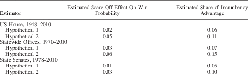
Table 3 presents the calculations that translate the results in Table 2 into estimates of the percentage of the party incumbency advantage that can possibly be attributed to scare-off. As in Table 2, the top panel covers the US House, the middle panel covers statewide offices, and the bottom panel covers state senate seats.
Estimates of the Scare-Off Effect

The first column multiplies each hypothetical estimate for the win-probability return to experience by the estimated difference in quality caused by incumbency in the relevant electoral context. The second column divides the first column by the estimated incumbency advantage for the given electoral context.
In order to get a sense of how much of the party incumbency advantage can be plausibly attributed to scare-off, we need estimates of the electoral effect of prior officeholder experience. How much larger is a party’s probability of winning a race, or expected vote percentage, if it fields an experienced candidate rather than an inexperienced one? Our RD approach does not yield such estimates, so we borrow from the literature. Previous estimates indicate that the value of prior officeholder experience is sizable, but probably about half as large as the value of incumbency, or lower.
For example, estimates from Canes-Wrone et al. (Reference Canes-Wrone, Brady and Cogan2002) imply that experienced US House challengers reduce the incumbents’ probability of winning by about 18 percentage points in “marginal” districts.Footnote 18 Using data on US House elections from 1946–86, Jacobson (Reference Jacobson1989) estimates that having an experienced candidate increases the challenging party’s probability of defeating a US House incumbent by 10 to 16 percentage points, depending on the “baseline” probability of winning—that is, the probability of winning without an experienced challenger.Footnote 19 The largest estimate is for the case where the baseline probability of winning is 25 percent. As we show below in Table 1, the party losing at time t wins at time t+1 only about 25–30 percent of the time, so the 25 percent baseline probability is in the relevant range. Jacobson (Reference Jacobson1989) also estimates that having an experienced candidate increases the challenging party’s expected vote percentage by 2.8 percentage points, again studying the US House from 1946–86.Footnote 20
Cox and Katz (Reference Cox and Katz1996) present separate estimates of the “quality effect” for each election year, for US House elections over the period 1946–90. The average of these estimates implies that having an experienced candidate increases a party’s expected vote percentage by 3.0 percentage points.Footnote 21 Studying the US Senate, Abramowitz and Segal (Reference Abramowitz and Segal1992) estimates that an experienced challenger gains ~2 percentage points of vote share relative to an inexperienced challenger.Footnote 22
We generate two hypothetical estimates of the return to candidate officeholder experience. The first, “Hypothetical 1,” is based on the estimates of the return to experience from the literature. For each setting, we take our estimate of the incumbency advantage (in terms of win probability) and divide by 2. This is, in essence, supposing that candidate experience is “half as good” as incumbency. There are two advantages to distilling the previous literature into this hypothetical estimate. First, it allows us to apply a tailored hypothetical to all three electoral contexts (since we have incumbency advantage estimates for each context), even though published estimates do not perfectly match up to those we study.Footnote 23 Second, it ensures that we compare apples-to-apples. Estimates such as those in Jacobson (Reference Jacobson1989) employ a counterfactual comparison between elections with an incumbent versus open elections, while the RD estimate compares cases with a Democratic incumbent to those with a Republican incumbent. By using an RD-based estimate for Hypothetical 1, we ensure that we are using our estimate of the scare-off effect in conjunction with an analogous estimate of quality’s effect on electoral outcomes.Footnote 24
In the second hypothetical estimate, “Hypothetical 2,” we make the even more unlikely assumption that being experienced is “as good as” incumbency, that is, that the return to experience is equal to the return to incumbency. This is almost certainly a large overestimate of the value of experience.
With these hypotheticals in hand, we then take the point estimate from row 1, column 4 of Table 2, 0.11, as the expected difference in candidate experience at time t+1. Multiplying this by our hypothetical returns to experience gives an estimate of the expected difference in the probability of winning at time t+1 that is due to the expected difference in candidate experience at time t+1 produced by the election outcome at time t. For Hypothetical 1 this is just 2 percent, as shown in row 1, column 1 of Table 3.
In the second column we divide this by the estimated party incumbency advantage, from column 1 of Table 2. We see that, given our estimate of the change in the candidate experience differential and the hypothetical estimate of the return to experience, scare-off only explains 6 percent of the overall incumbency advantage in terms of win probability.
The calculations for the other two electoral contexts show consistent results. Across the three cases, scare-off is estimated to explain 5–7 percent of the overall incumbency advantage. Even when using the unrealistic hypothetical (Hypothetical 2), we still find that scare-off only explains 10–15 percent of the advantage.
The difference in the experience differential caused by incumbency is simply not enough to produce the incumbency advantage we observe among these close races, regardless of the return to experience. Consider the US House estimates. Even if we use a more generous estimate for the effect of incumbency on the net experience differential—by taking the right upper bound of the confidence interval for the estimate, which is 0.30, we still find that scare-off only explains 15 percent of the advantage under Hypothetical 1, and only 30 percent under the unrealistic Hypothetical 2.
In the Appendix, we replicate the analysis using vote share as the dependent variable, finding consistent results. In all three contexts, scare-off is estimated to generate less than a percentage-point of extra vote share using Hypothetical 1. Even under Hypothetical 2, scare-off is only estimated to bring as much as 1.52 percentage points in vote share (in statewide offices).
Long-Term Effects
Thus far we have established a surprisingly small amount of scare-off of candidates with previous officeholder experience, even in contexts where the incumbency advantage is quite large. One possible explanation is that candidate entry decisions are “sticky,” such that incumbency status at time t occurs too late to influence a candidate’s decision in the very next race. Or, in a similar vein, if the incumbency advantage increases with terms in office, the size of the scare-off effect might grow with time, such that experienced challengers are not scared off after an initial election result in an open seat, but are scared off by incumbents who accrue multiple terms of service. This might especially be the case for the close races at time t that we investigate.
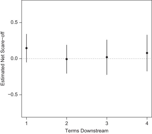
To test for the possibility of a “long term” scare-off effect, we re-estimate Equation (1) with outcome variables further downstream.Footnote 25 In particular, we replace Net Cand Experience t+1 with its observations at t+2, t+3, and t+4, where t indexes terms. We focus on statewide offices since here we can easily look downstream without having to confront redistricting. We keep our main specification, local linear OLS estimated separately on each side of the discontinuity in a 5 percent bandwidth, and we plot the resulting estimates in Figure 4.
Estimated Downstream Scare-off, Statewide Offices Notes: Plots regression discontinuity estimates of the effect of incumbency on future net candidate quality. The leftmost estimate reproduces that reported in Table 2, showing that there is no immediate scare-off of candidates with previous officeholder experience. As the next points show, there is no downstream scare-off either.

As the figure shows, we find no evidence of any downstream scare-off of experienced candidates. The first estimate, at one term downstream, reproduces the estimate from Table 2. Looking across the figure, we see that the RD estimates at t+2, t+3, and t+4 are equally small (or even smaller).Footnote 26 Experienced candidates are not scare-off by incumbency in close statewide races either now or in the future.
Discussion
The sources of the large incumbency advantage in American elections, and the consequences it has for our system of representation, are still obscure. If the very fact that an experienced politician already possesses a seat deters quality candidates from stepping forward and running for office, then the incumbency advantage may provide poor incentives for elected officials, furnishing them with an electoral bonus regardless of their actions in office.
However, in this paper we find that this “scare-off” phenomenon is almost non-existent in US elections, at least in closely-contested seats. Since these same seats exhibit a large advantage to incumbents, we can conclude that scare-off is not a necessary condition for an incumbency advantage. We can also suggest that it plays only a small role in the advantage in other US contexts as well.
There are two main complications to interpreting our RD estimates, but neither is problematic in the present instance. First, as is well-known, the RD focuses on the effect of “party” incumbency, in the sense that the treatment is defined to be the assignment of Democratic incumbency, rather than focused on the individual legislator (who may or may not run again in the subsequent election). We are not overly concerned with this issue because the important effects of scare-off—namely, its role in altering the incentives of politicians—hold regardless of whether the scare-off comes from individual incumbency or party incumbency. Moreover, Fowler and Hall (Reference Fowler and Hall2015) present evidence that party incumbency status conveys no electoral advantage separate from individual incumbency, at least in state legislatures. As a result it is likely that our estimates capture almost entirely effects related to individual incumbency, anyways.
Second, the RD estimates apply only in close elections and do not speak directly to potential scare-off effects in lopsided districts. In the present setting this issue of external validity is less of a concern, because for many questions we are most interested in competitive districts. Competitive districts are those in which electoral turnover is likely; electoral security from scare-off is thus most consequential in these districts, where there is a real chance for a quality challenger to obtain office in the absence of scare-off. In addition, as we discussed in the Introduction, it is not so obvious that the scare-off effect ought to be larger in safer districts.
This is not to say that potential challengers are not strategic. However, we must understand the extent and limits to such strategic behavior. Tables such as the those in [Jacobson (Reference Jacobson1989, Reference Jacobson2009)] show mainly that underlying district partisanship has a large effect on the probability the challenger is experienced. This reflects both the strategic decisions of candidates about whether or not to run and also the “pool” of available experienced candidates. In a heavily Democratic US House district, most of the lower offices will also be held by Democrats, not Republicans. The tables in Jacobson and Kernell (Reference Jacobson and Kernell1983) and Banks and Kiewiet (Reference Banks and Kiewiet1989) show large average differences in candidate quality in open-seat races versus incumbent-contested races, but even these statistics mix incumbency status with district type. On average, incumbents are running in districts that are quite safe for their party, while open-seat races tend to occur more often in competitive districts. It is difficult to know which factor—district competitiveness or incumbency status—is more important. When they control for both factors, Hirano and Snyder (Reference Hirano and Snyder2009) find little evidence that scare-off is produced by incumbency per se (at least in state legislative races), especially in competitive districts.
Why is there so little scare-off in these competitive districts or states with close elections? We can only speculate at present. We suspect that the actual dynamics underlying the decision for a quality candidate to run for higher office are more complicated than a simple scare-off story can capture. Although avoiding an entrenched incumbent might well be a factor weighing against a run for office, a quality candidate must consider other factors as well. If she runs this year, will she have to give up her current office? If she does not challenge the incumbent this year, can she afford to wait? Elections for many local offices, for example, are in odd-numbered years. For the politicians holding those offices the opportunity cost of challenging an incumbent in a higher office is relatively low. Many lower offices also have term limits, and expiring candidates may have few other appetizing political options besides “moving up.” These are just some of the reasons we might expect scare-off to be less “scary” than is often supposed.
Appendix
A.1 Vote Share Analysis
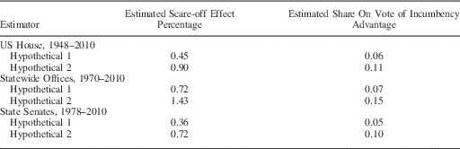
In Table A1, we present the RD estimates following the same form as Equation (1) with the Democratic percentage of the two-party vote at time t+1 as the outcome variable. As expected, we find a large vote-share incumbency advantage across all three contexts. In Table A2, we again calculate the share of the incumbency advantage explained by scare-off, using the same estimates of the experience differential from Table 2.
Incumbency and Vote Share

Vote-Share Estimates of the Scare-Off Effect

Again, we generate two hypothetical returns to quality, specific to each electoral context. In “Hypothetical 1” we again suppose that candidate quality is “half as good as” our estimate for the vote-share return to incumbency, and in “Hypothetical 2” we again assume it is “as good as” our estimate for the vote-share return to incumbency. In the first column, we multiply the hypothetical returns to quality by the effect of incumbency on the net experience differential. In all three cases, scare-off is estimated to generate less than a percentage-point of extra vote share using Hypothetical 1. Even under the extreme Hypothetical 2, scare-off is only estimated to bring as much as 1.52 percentage points in vote share (in statewide offices).
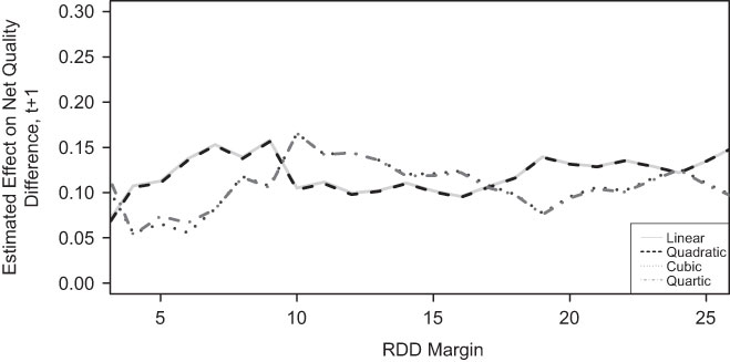
Robustness of regression discontinuity (RD) Estimate, US House Notes: The four lines in the plot represent the RD estimate from Equation (1) using a linear, quadratic, cubic, and quartic specification of the running variable, respectively, across bandwidths.

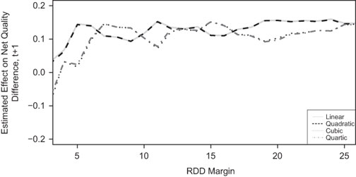
Robustness of regression discontinuity (RD) estimate, statewide offices Notes: The four lines in the plot represent the RD estimate from Equation (1) using a linear, quadratic, cubic, and quartic specification of the running variable, respectively, across bandwidths.

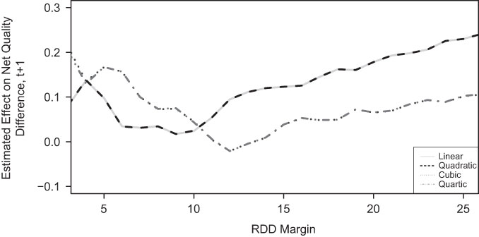
Robustness of regression discontinuity (RD) estimate, state senates Notes: The four lines in the plot represent the RD estimate from Equation (1) using a linear, quadratic, cubic, and quartic specification of the running variable, respectively, across bandwidths.

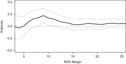
Regression discontinuity designs balance at time t: US House Notes: Equation (2) is reestimated at the indicated bandwidths, always using the local linear regression estimated separately on each side of the discontinuity. The graph plots the resulting estimates across bandwidths, along with 95 percent confidence intervals from robust standard errors.

Regression discontinuity designs balance at time t: statewide offices Notes: Equation (2) is reestimated at the indicated bandwidths, always using the local linear regression estimated separately on each side of the discontinuity. The graph plots the resulting estimates across bandwidths, along with 95 percent confidence intervals from robust standard errors.

Regression discontinuity designs balance at time t: state senates Notes: Equation (2) is reestimated at the indicated bandwidths, always using the local linear regression estimated separately on each side of the discontinuity. The graph plots the resulting estimates across bandwidths, along with 95 percent confidence intervals from robust standard errors.

A.2 Calculating the Scare-Off Effect in the RD Framework
Interpreting scare-off in the RD framework is slightly complicated. This Appendix justifies the calculations in the text—in particular, it clarifies an apparent “double counting” issue. The derivation is similar to that in Erikson and Titiunik (Reference Erikson and Titiunik2015).
First, consider δ NQD, the RD estimator for the effect of incumbency on the net quality differential (NQD) between the two parties. This is defined as:
 $$\delta _{{NQD}} =(E[Q_{{t{\plus}1}}^{{\rm D}} \!\mid\!W_{t}^{{\rm D}} =1]{\minus}E[Q_{{t{\plus}1}}^{{\rm R}} \!\mid\!W_{t}^{{\rm D}} =1]){\minus}(E[Q_{{t{\plus}1}}^{{\rm D}} \!\mid\!W_{t}^{{\rm D}} =0]{\minus}E[Q_{{t{\plus}1}}^{{\rm R}} \!\mid\!W_{t}^{{\rm D}} =0]),$$
where
 $$Q_{{t{\plus}1}}^{{\rm D}} $$
and
 $$Q_{{t{\plus}1}}^{{\rm R}} $$
are dummies for Democratic and Republican quality
candidates at t+1, and
 $$W_{t}^{{\rm D}} $$
is an indicator for Democratic victory in the election
at time t. Let
 $$\gamma _{{\rm D}} =E[Q_{{t{\plus}1}}^{{\rm D}} \!\mid\!W_{t}^{{\rm D}} =1]{\minus}E[Q_{{t{\plus}1}}^{{\rm D}} \!\mid\!W_{t}^{{\rm D}} =0]$$
and
 $$\gamma _{{\rm R}} =E[Q_{{t{\plus}1}}^{{\rm R}} \!\mid\!W_{t}^{{\rm D}} =0]{\minus}E[Q_{{t{\plus}1}}^{{\rm R}} \!\mid\!W_{t}^{{\rm D}} =1]$$
denote party-specific effects of incumbency on the
candidate quality differential, noting that the conditions are reversed
for γ
R since
 $$W_{t}^{{\rm R}} =1{\minus}W_{t}^{{\rm D}} $$
. We are interested in the overall change in quality
caused by incumbency, that is, the average of the party-specific effects,
γ=(γ
D+γ
R)/2. Note that we can rewrite the above equation
as:
 $$\eqalignno{ \delta _{{{\rm NQD}}} & =(E[Q_{{t{\plus}1}}^{{\rm D}} \!\mid\!W_{t}^{{\rm D}} =1]{\minus}E[Q_{{t{\plus}1}}^{{\rm D}} \!\mid\!W_{t}^{{\rm D}} =0]){\plus}(E[Q_{{t{\plus}1}}^{{\rm R}} \!\mid\!W_{t}^{{\rm D}} =0]{\minus}E[Q_{{t{\plus}1}}^{{\rm R}} \!\mid\!W_{t}^{{\rm D}} =1]) \cr & =\gamma _{{\rm D}} {\plus}\gamma _{{\rm R}} \cr & =2\gamma . $$
Next, consider δ WD, the RD estimator for the effect of incumbency on the probability of winning the next election. This is defined as:
 $$\delta _{{{\rm WD}}} =E[W_{{t{\plus}1}}^{{\rm D}} \!\mid\!W_{t}^{{\rm D}} =1]{\minus}E[W_{{t{\plus}1}}^{{\rm D}} \!\mid\!W_{t}^{{\rm D}} =0].$$
Although it makes no difference for the actual estimate,
it is intuitive to think about these effects as deviations from a 50
percent win probability. Let
 $$\theta _{{\rm D}} =E[W_{{t{\plus}1}}^{{\rm D}} {\minus}0.5\!\mid\!W_{t}^{{\rm D}} =1]$$
and
 $$\theta _{{\rm R}} =E[W_{{t{\plus}1}}^{{\rm R}} {\minus}0.5\!\mid\!W_{t}^{{\rm R}} =1]$$
be the party-specific incumbency effects. Again, we are
interested in the average, θ=(θ
D+θ
R)/2. Note that
 $$\eqalignno{ \delta _{{{\rm WD}}} & =E[W_{{t{\plus}1}}^{{\rm D}} {\minus\,}0.5\!\mid\!W_{t}^{{\rm D}} =1]{\minus}E[W_{{t{\plus}1}}^{{\rm D}} {\minus}\,0.5\!\mid\!W_{t}^{{\rm D}} =0] \cr &=E[W_{{t{\plus}1}}^{{\rm D}} {\minus}\,0.5\!\mid\!W_{t}^{{\rm D}} =1]{\minus}E[0.5\,{\minus}W_{{t{\plus}1}}^{{\rm R}} \!\mid\!W_{t}^{{\rm D}} =0] \cr &=E[W_{{t{\plus}1}}^{{\rm D}} {\minus}\,0.5\!\mid\!W_{t}^{{\rm D}} =1]{\plus}E[W_{{t{\plus}1}}^{{\rm R}} {\minus}\,0.5\!\mid\!W_{t}^{{\rm D}} =0] \cr &=\theta _{{\rm D}} {\plus}\theta _{{\rm R}} \cr &=2\theta $$
Thus, both of the RD estimates give us twice the average of the party effects. Define our estimate for the share of the incumbency advantage resulting from scare-off as β=A·δ NQD/δ WD where A is the return to quality. Then,
 $$\beta ={{A \cdot 2\gamma } \over {2\theta }}={{A\gamma } \over \theta }$$
Thus, given an estimate for the return to quality, A, the “double counting” phenomenon cancels out in our calculation of the share of the incumbency advantage resulting from the scare-off effect.
A.3 Robustness of RD Estimate
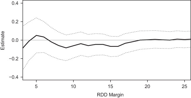
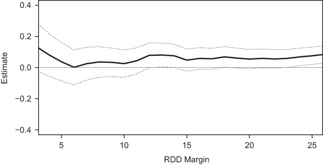
The following three figures show the stability of the RD estimate across bandwidth sizes and specifications of the forcing variable. Each plot shows the estimates from Equation (1) using Net Cand Experience as the outcome variable.Footnote 27 The four lines in the plot represent the estimate using a linear, quadratic, cubic, and quartic specification of the running variable, respectively. The sparsity of data within very small bandwidths makes estimates noisy, so we start the plots at a 4 percent bandwidth. We end the plots at 25 percent, already a much larger bandwidth than commonly used in the literature. That said, estimates remain somewhat stable beyond this point, although local linear estimates in particular begin to increase as specification bias grows.
As the plots show, estimates are extremely stable (Figures A1–A3).
A.4 Balance Tests for RD
The key identifying assumption of the RD design is that candidates at time t cannot “sort” across the discontinuity. This assumption is plausible on substantive grounds because it is almost impossible to predict close elections (making it exceedingly unlikely that candidates could identify when they are in a close election and then differentially exert effort to produce sorting). In this section, we offer supportive evidence for the validity of the RD, following best practices (e.g., Caughey and Sekhon Reference Caughey and Sekhon2011; Eggers et al. N.d.).
First, in Table A3 we present balance tests at the exact bandwidth and specifications of the results reported in the paper (5 percent bandwidth, local linear estimated separately on each side of the equation). The equation to be estimated is:
 $$Y_{{i,t}} =\beta \,Democ\,Win_{{it}} {\plus}f(Democ\,Vote\,Pct_{{it}} ){\plus}\epsilon _{{it}} ,$$
which is identical to Equation (1) in the body of the paper, except that the outcome is the already-realized quality of the candidates in the close election at time t. For simplicity, we focus on the NQD for the tests below.
As we see in Table A3, there is no evidence of imbalances in the NQD at time t. That is to say, the NQD at time t in elections in which the Democrat barely wins does not appear to differ from the NQD in close elections at time t in which the Democrat barely loses. This supports the notion that candidates are not sorting across the discontinuity.
In addition to Table A3, we also present figures showing the balance tests across bandwidths for the three electoral contexts. In each figure, Equation (2) is reestimated at the indicated bandwidths, always using the local linear regression estimated separately on each side of the discontinuity. The graphs plot the resulting estimates across bandwidths, along with 95 percent confidence intervals from robust standard errors. As can be seen, there is no evidence of sorting in any of the three contexts. In the US House graph, there is a range in which the estimate is positive and statistically significant, but it is well outside the bandwidths reported in the paper and, tellingly, disappears as more data is added (as the bandwidth increases). Note that no standard errors are adjusted for multiple testing, so we would expect to reject the null occasionally (like in that region) by chance (Table A3; Figures A4–A6).
Balance Tests for Regression Discontinuity Designs