1. Introduction
Turbulent thermal convection driven by a mean temperature gradient between impermeable horizontal plates, known as Rayleigh–Bénard convection (RBC), commonly exhibits spatio-temporal coherence in the form of a large-scale circulation (LSC). This large-scale mean flow consists of one or several roll structures which span the entire height of the convective layer (Krishnamurti & Howard Reference Krishnamurti and Howard1981; Sano, Wu & Libchaber Reference Sano, Wu and Libchaber1989; Ciliberto, Cioni & Laroche Reference Ciliberto, Cioni and Laroche1996; Niemela et al. Reference Niemela, Skrbek, Sreenivasan and Donnelly2001; Xia, Sun & Zhou Reference Xia, Sun and Zhou2003). The driving of the LSC can largely be ascribed to the clustering of coherent regions of warm and cold fluid, i.e. thermal plumes that detach from the horizontal boundary layers and that are the main carriers of the advective heat flux (Kadanoff Reference Kadanoff2001). It has been shown in experiments of RBC in water (Zocchi, Moses & Libchaber Reference Zocchi, Moses and Libchaber1990; Qiu & Tong Reference Qiu and Tong2002) that the clustering and collective alignment of thermal plumes is mainly caused by boundary layer perturbations due to the impingement of warm (cold) plumes on the top (bottom) wall. Parodi et al. (Reference Parodi, von Hardenberg, Passoni, Provenzale and Spiegel2004) come to a similar conclusion and further suggest that the clustering of plumes induces a slow upscale energy transfer, eventually creating the slowly evolving mean LSC flow. Experiments at the onset of convection by Xi, Lam & Xia (Reference Xi, Lam and Xia2004) support this picture.
However, they also show that, before the largest scales of the flow have reached the height of the convection layer, a different structure of heat transport prevails. This regime is not dominated by boundary layer perturbations and the resulting LSC but rather by localised buoyant interactions and the potentially universal nonlinear small-scale dynamics of convective turbulence. Convective flows of this kind are, e.g. relevant for processes in atmospheres or stellar convection zones (Celani et al. Reference Celani, Mazzino, Seminara and Tizzi2007; Garaud et al. Reference Garaud, Ogilvie, Miller and Stellmach2010; Rosenblum et al. Reference Rosenblum, Garaud, Traxler and Stellmach2011), under the assumption that the dynamics is governed by the bulk flow instead of boundary layers. Such geo- and astrophysical configurations are experimentally and numerically approximated by avoiding or reducing the formation of kinetic and thermal boundary layers. An experimental implementation of this strategy uses two fluid reservoirs connected by a vertical pipe or channel, where turbulence is driven by an unstable density or temperature gradient between the reservoirs (Cholemari & Arakeri Reference Cholemari and Arakeri2005, Reference Cholemari and Arakeri2009; Gibert et al. Reference Gibert, Pabiou, Chillà and Castaing2006, Reference Gibert, Pabiou, Tisserand, Gertjerenken, Castaing and Chillà2009; Pawar & Arakeri Reference Pawar and Arakeri2016). In numerical simulations, the absence of confining boundaries can be approximated by employing periodic boundary conditions. In addition, a constant mean temperature gradient is imposed along the vertical, defined by the direction of gravitational acceleration. Such homogeneous Rayleigh–Bénard (HRB) set-ups have been used to confirm asymptotic scaling predictions in strongly buoyancy-driven, turbulent convection (Kraichnan Reference Kraichnan1962; Lohse & Toschi Reference Lohse and Toschi2003; Calzavarini et al. Reference Calzavarini, Lohse, Toschi and Tripiccione2005), to study Lagrangian turbulence statistics (Pratt et al. Reference Pratt, Busse, Müller, Watkins and Chapman2017, Reference Pratt, Busse and Müller2020) and to investigate the small-scale structure of velocity and temperature fluctuations (Biskamp & Schwarz Reference Biskamp and Schwarz1997; Biskamp et al. Reference Biskamp, Hallatschek and Schwarz2001a ; Celani et al. Reference Celani, Matsumoto, Mazzino and Vergassola2002; Biferale et al. Reference Biferale, Calzavarini, Toschi and Tripiccione2003). However, in these HRB systems (Calzavarini et al. Reference Calzavarini, Doering, Gibbon, Lohse, Tanabe and Toschi2006) and related physical configurations such as homogeneous salt-finger convection (Xie et al. Reference Xie, Miquel, Julien and Knobloch2017, Reference Xie, Julien and Knobloch2019), the lack of confinement of the flow can give rise to elevator instabilities, creating strong vertical shear flows. Since these are detrimental to statistical homogeneity, their suppression can be enforced via explicit elimination of vertical mean velocities (Moll et al. Reference Moll, Pietarila Graham, Pratt, Cameron, Müller and Schüssler2011), rendering the systems quasi-periodic, or by large-scale damping (see below). The above-mentioned complications that arise in fully periodic convection limit the direct comparability of RBC and HRB systems and require careful and comprehensive consideration of parameter regimes and nonlinear interdependencies. In the present work, no such comparison is intended, apart from more general aspects that might be helpful to obtain a broader perspective on the problem considered here. We regard appropriately stabilised statistically homogeneous convection as an idealised approximation to convection with negligible boundary effects.
While the structure of heat transport in RBC with a dominant LSC has been the subject of numerous studies (Hartlep, Tilgner & Busse Reference Hartlep, Tilgner and Busse2003; Xia et al. Reference Xia, Sun and Zhou2003; Hartlep, Tilgner & Busse Reference Hartlep, Tilgner and Busse2005; Shishkina & Wagner Reference Shishkina and Wagner2007; Emran & Schumacher Reference Emran and Schumacher2015; Schneide et al. Reference Schneide, Pandey, Padberg-Gehle and Schumacher2018; Blass et al. Reference Blass, Verzicco, Lohse, Stevens and Krug2021), comparable work on buoyancy-driven convective turbulence absent LSC is scarce. Axially homogeneous experiments by Cholemari & Arakeri (Reference Cholemari and Arakeri2009) indicate that the most prominent buoyant interactions are collisions of upward- and downward-moving thermal plumes. Visualisations in Pawar & Arakeri (Reference Pawar and Arakeri2016) suggest that the interaction of thermal plumes induces vortices on large to intermediate spatial scales. Similarly, visualisations of a two-dimensional HRB simulation (Celani et al. Reference Celani, Matsumoto, Mazzino and Vergassola2002) indicate such a plume-induced vortical structure.
The present study aims at substantiating those findings with an exploration of the spatial structure of turbulent convective heat transport in two-dimensional, periodic HRB convection. The investigation is based on two-dimensional pseudospectral direct numerical simulations of the Boussinesq equations from the moderately nonlinear regime up to highly turbulent convection in a range of Rayleigh numbers
 $10^6 \lt {\textit{Ra}} \lt 10^{12}$
. Both Eulerian and Lagrangian measurements are utilised in order to characterise the dominant mode of large-scale transport, which leads to a reduced description of the flow and a better understanding of its salient properties. The remainder of this paper is structured as follows. Section 2 presents numerical experiments and underlying theory. In § 3 the system is analysed with respect to its configuration space and spectral characteristics and subsequently in § 4 a Lagrangian description of coherent transport is proposed. In § 5 the transport structure, its imprint on mean field quantities and its universal character are analysed based on a reduced description. Finally, § 6 summarises the findings. A set of test simulations including pertinent diagnostics is briefly discussed in Appendix A to clarify role and impact of the large-scale damping mechanism employed in the present simulations.
2. Governing equations
We consider a two-dimensional incompressible fluid in a periodic square of edge length
 $L = 2\pi$
and area
 $A$
, which is subject to a linear background temperature stratification,
 $\bar {T}(y)$
, i.e. a constant temperature gradient along the y-direction,
 $\boldsymbol{\nabla }\bar {T} (y) = \text{const.}$
Constant gravitational acceleration
 $\boldsymbol{g} = (0,-g)^T$
is present such that
 \begin{equation} \boldsymbol{g}\boldsymbol{\cdot }\boldsymbol{\nabla }\bar {T} \gt 0, \end{equation}
rendering the fluid unstably stratified, i.e. prone to self-sustained convective motion, where heat is advectively transported along the direction of
 $-\boldsymbol{\nabla }\bar {T}$
. The two-dimensional motion, defined by the velocity components
 \begin{align} u_1 (\boldsymbol{r},t) = u_1(x,y,t), \quad u_2 (\boldsymbol{r},t) = u_2(x,y,t), \quad u_3 (\boldsymbol{r},t) = 0, \end{align}
is coupled to the temperature fluctuations
 $\theta (x,y,t) = T(x,y,t) - \bar {T}(y)$
via the Boussinesq equations of thermal convection, given in dimensionless form as
 \begin{align} \partial _t \boldsymbol{u} + (\boldsymbol{u} \boldsymbol{\cdot }\boldsymbol{\nabla }) \boldsymbol{u} &= -\boldsymbol{\nabla }\!p +\tilde {\nu } \Delta \boldsymbol{u} + \beta _{\boldsymbol{u}} (\Delta )^{-1} \boldsymbol{u} + \boldsymbol{e}_y \theta , \end{align}
 \begin{align} \partial _t \theta + (\boldsymbol{u} \boldsymbol{\cdot }\boldsymbol{\nabla }) \theta &= \tilde {\kappa } \Delta \theta + \beta _{\theta } (\Delta )^{-1} \theta + \boldsymbol{e}_y \boldsymbol{\cdot }\boldsymbol{u}, \end{align}
 \begin{align} \boldsymbol{\nabla }\boldsymbol{\cdot }\boldsymbol{u} &= 0, \end{align}
where
 $p$
is the pressure,
 $\beta_{\boldsymbol{u}}$
and
 $\beta_{\theta}$
are the large-scale damping coefficients and
 $\boldsymbol{e}_y$
is the unit vector along the y-direction. The dissipation coefficients,
 $\tilde{\nu}$
and
 $\tilde{\kappa}$
, denote the dimensionless kinematic viscosity and thermal diffusivity, respectively. Incompressible dynamics is enforced numerically by solving for the curl of the velocity,
 $\boldsymbol{\omega } = \boldsymbol{\nabla }\times \boldsymbol{u}$
, which for two-dimensional motion reduces to the pseudo-scalar vorticity
 $\omega (\boldsymbol{r},t) = \omega _3 (x,y,t)$
governed by
 \begin{equation} \partial _t \omega + (\boldsymbol{u} \boldsymbol{\cdot }\boldsymbol{\nabla }) \omega = \tilde {\nu } \Delta \omega + \beta _u (\Delta )^{-1} \omega + \partial _x \theta . \end{equation}
The equations are made dimensionless by using the characteristic domain size,
 $L$
, and the integral buoyancy time scale,
 $t_b = (\alpha g |\partial _y \bar {T}|)^{-1/2}$
, with
 $\alpha$
the thermal expansion coefficient at constant pressure. Large-scale damping of temperature fluctuations and velocity is introduced via inverse Laplacian terms with coefficients
 $\beta _u = \beta _{\theta } = 3$
for all simulations. For two-dimensional turbulence in a finite volume as in the present set-up, this is necessary to prevent an accumulation of energy at the largest scales due to the inverse turbulent cascade of kinetic energy (Kraichnan Reference Kraichnan1967). Please note that this approach does not eliminate the inverse cascade of kinetic energy on smaller spatial scales. As a beneficial side effect, the artificial energy sink also suppresses linearly unstable elevator solutions, i.e. oppositely directed vertical streamers, induced by vertical periodicity along the direction of gravity (see Calzavarini et al. (Reference Calzavarini, Lohse, Toschi and Tripiccione2005, Reference Chen, Ecke, Eyink, Rivera, Wan and Xiao2006) regarding the instability and e.g. Biskamp et al. (Reference Biskamp, Hallatschek and Schwarz2001b
) and Müller et al. (Reference Müller, Malapaka and Busse2012) for additional applications of the employed large-scale damping). We note that a similar large-scale stabilisation of elevator modes is realised in an asymptotically valid reduced model of homogeneous salt-finger convection via the coupling of fluid momentum to the stable large-scale temperature field (Xie, Julien & Knobloch Reference Xie, Julien and Knobloch2019). Alternative techniques of elevator-mode suppression are applied in e.g. Moll et al. (Reference Moll, Pietarila Graham, Pratt, Cameron, Müller and Schüssler2011), Barral & Dubrulle (Reference Barral and Dubrulle2023). The specific values of
 $\beta _u$
and
 $\beta _\theta$
represent a compromise between the energetic stabilisation on the largest scales of the flow and a minimal impact on the spectral energy of smaller-scale fluctuations. This allows for a straightforward establishment of a statistically steady state of the flow (see Appendix A for details regarding the influence of large-scale damping and the present choice of parameters). We would like to point out that the elevator mode, as an exact solution of the governing equations, is driven by the physical convective large-scale instability of the system, which certainly plays an important role in shaping the flow’s general dynamics. Therefore, we regard only a non-saturated elevator instability as spurious. From this perspective, the applied large-scale damping models the stabilising interaction of larger-scale turbulent fluid motion in the vicinity of a growing elevator solution or, for example, the effect of stabilising boundary conditions. In the dimensionless system of equations the diffusive parameters
 $\tilde {\nu }$
and
 $\tilde {\kappa }$
are expressed in terms of the nominal Rayleigh number
 $\textit{Ra} = \alpha g |\partial _y \bar {T}| L^4 / \nu \kappa$
and the Prandtl number
 $\textit{Pr} = \nu / \kappa$
as
 $\tilde {\nu } = (2\pi )^2 (\textit{Pr}/\textit{Ra})^{1/2}$
and
 $\tilde {\kappa } = (2\pi )^2 (1/\textit{Pr}\textit{Ra})^{1/2}$
. The Rayleigh number relates the energy dissipation due to diffusivity of momentum and temperature with the maximal available thermal energy contained in the temperature fluctuations (see Busse Reference Busse1978, chapter 2.1). Although it is, strictly speaking, not well defined for a homogeneous system, the present work uses
 ${\textit{Ra}}$
as an illustrative parameter expressing the dynamical impact of buoyant forces. The resulting nonlinear spatial transports of heat and momentum are quantified by the Nusselt number (Nu) and the Reynolds number (Re), respectively. The former parameter, defined as
 ${\textit{Nu}} = \langle u_y \theta \rangle _{\textit{A}\text{,}\textit{t}} / \tilde {\kappa } |\boldsymbol{\nabla }\bar {T}| + 1$
, with
 $\langle \boldsymbol{\cdot }\rangle _{\textit{A}\text{,}\textit{t}}$
denoting the spatio-temporal average, represents the relation of combined nonlinear convective and diffusive heat flux to purely diffusive heat flux. The latter parameter, defined as
 ${\textit{Re}} = L \sigma _u / \tilde {\nu }$
, with
 $\sigma$
denoting the standard deviation, characterises the ratio of advective and viscous momentum transports. As first shown by Lohse & Toschi (Reference Lohse and Toschi2003) and later confirmed by Calzavarini et al. (Reference Calzavarini, Lohse, Toschi and Tripiccione2005), HRB convection exhibits a scaling regime
 ${\textit{Nu}} \sim {\textit{Ra}}^{1/2}$
and
 ${\textit{Re}} \sim \textit{Ra}^{1/2}$
consistent with Kraichnan’s asymptotic predictions for very large Rayleigh numbers (Kraichnan Reference Kraichnan1962) in the classical wall-bounded Rayleigh–Bénard system.
Parameters of the simulation runs S1–S7. The columns from left to right show the simulation number, the nominal Rayleigh number, the number of collocation points, the dimensionless viscous and thermal diffusion parameters, the Nusselt number and the Reynolds number.

Figure 1 shows
 ${\textit{Nu}}({\textit{Ra}})$
and
 ${\textit{Re}}({\textit{Ra}})$
for the seven simulation runs (S1–S7) considered in this paper, where
 ${\textit{Ra}}$
is varied via
 $\tilde {\nu }$
and
 $\tilde {\kappa }$
. In agreement with previous studies, the numerical data match the theoretical scaling well. The parameters for each simulation are summarised in table 1. The number of collocation points N is chosen such that the condition
 $k_{\textit{max}} \eta \geqslant 1.5$
holds (Pope Reference Pope2001, § 9.2.1), where
 $k_{\textit{max}}$
is the largest wavenumber resolved on the numerical grid and
 $\eta =(\tilde {\nu }^3/\varepsilon )^{1/4}$
is the Kolmogorov length scale defined with the dissipation rate
 $\varepsilon$
of kinetic energy. This is sufficient as in the present work
 $\eta$
is approximately equal to or smaller than the corresponding dissipation length of the temperature fluctuations,
 $\eta _\theta =\tilde {\kappa }^{5/8}/\varepsilon _\theta ^{1/8}$
, in Bolgiano–Obukhov turbulence (cf. § 3.2), where
 $\varepsilon _{\theta}$
is the dissipation rate of thermal energy. All simulations in this work start from an initial state with small random temperature fluctuations around the scale
 $k \approx 0.8 k_{\textit{max}}$
and a quiescent velocity field. After reaching a statistically steady state, the equations are integrated in time for a further
 $120 t_b$
in order to ensure statistical convergence. For all simulations the effective Prandtl number,
 $\textit{Pr} = \tilde {\nu } / \tilde {\kappa }$
, is unity, except for S7, where
 $\textit{Pr} = 0.625$
with the aim of optimising the small-scale spectral scaling behaviour given the resolution constraint for this simulation. The measurable effects of this deviation in the case of highest nominal Rayleigh and Reynolds numbers are expected to be negligibly small beyond the dissipative scales of the flow due to the dominance of the nonlinear and general thermal dynamics over linear dissipative terms.
Nusselt number (Nu, diamonds) and Reynolds number (Re, triangles) as a function of Rayleigh number for simulation runs S1–S7 (see table 1). The dashed lines mark the asymptotic scaling
 $\sim\! \textit{Ra}^{1/2}$
(cf. Kraichnan Reference Kraichnan1962).

Equations (2.4) and (2.6) are solved using a standard pseudospectral simulation code with 2/3-aliasing that previously has been employed for a study of two-dimensional hydrodynamic turbulence in Wang, Sesterhenn & Müller (Reference Wang, Sesterhenn and Müller2023). The last terms on the right-hand sides of (2.3) and (2.6) represent the coupling of the temperature field with the velocity and vorticity due to buoyancy. Owing to the prescribed alignment of gravity and mean temperature gradient, this coupling establishes a mean positive correlation between temperature and vertical velocity, which leads to an anisotropic mean injection of energy into the system. This is best shown in terms of the kinetic energy, thermal energy and enstrophy budgets, where all these quantities are normalised by a constant density,
 $\rho _0$
. In Fourier space, they are given as
 $\hat {E}_u (\boldsymbol{k}) = \hat {\boldsymbol{u}}^*(\boldsymbol{k}) \boldsymbol{\cdot }\hat {\boldsymbol{u}}(\boldsymbol{k})/2$
,
 $\hat {E}_{\theta } (\boldsymbol{k}) = \hat {\theta }^*(\boldsymbol{k}) \hat {\theta }(\boldsymbol{k})/2$
and
 $\hat {\varOmega }( \boldsymbol{k}) = \hat {\omega }^*(\boldsymbol{k}) \hat {\omega }(\boldsymbol{k})/2$
, respectively, where
 $\boldsymbol{k} = (k_x,k_y)^T$
is the two-dimensional wave vector and
 $^*$
denotes complex conjugation. Their evolution equations are derived from (2.3)–(2.6) as
 \begin{align} \partial _t \hat {E}_u (\boldsymbol{k}) &= \hat {T}_u(\boldsymbol{k}) - 2 \tilde {\nu } k^2 \hat {E}_u (\boldsymbol{k}) - 2 \beta _u k^{-2} \hat {E}_u (\boldsymbol{k}) + {\text{Re}} \big \{ \hat {u}_y^*(\boldsymbol{k}) \hat {\theta } (\boldsymbol{k}) \big \}, \end{align}
 \begin{align} \partial _t \hat {E}_{\theta } (\boldsymbol{k}) &= \hat {T}_{\theta } (\boldsymbol{k}) - 2 \tilde {\kappa } k^2 \hat {E}_{\theta } (\boldsymbol{k}) - 2 \beta _{\theta } k^{-2} \hat {E}_{\theta } (\boldsymbol{k}) + {\text{Re}}\big \{\hat {u}_y(\boldsymbol{k}) \hat {\theta }^* (\boldsymbol{k})\big \}, \end{align}
 \begin{align} \partial _t \hat {\varOmega } (\boldsymbol{k}) &= \hat {T}_{\omega } (\boldsymbol{k}) - 2 \tilde {\nu } k^2 \hat {\varOmega } (\boldsymbol{k}) - 2 \beta _{u} k^{-2} \hat {\varOmega } (\boldsymbol{k}) + k_x {\text{Re}} \big \{i \hat {\theta }(\boldsymbol{k})\hat {\omega }^*(\boldsymbol{k})\big \}, \end{align}
where Re denotes the real part of the argument and
 $\hat {T}_{(\boldsymbol{\cdot })} (\boldsymbol{k})$
are nonlinear transfer terms that conservatively redistribute energy and enstrophy among Fourier modes. They are given as (cf. e.g. Pope Reference Pope2001 and Verma, Kumar & Pandey Reference Verma, Kumar and Pandey2017)
 \begin{align} \hat {T}_u (\boldsymbol{k}) &= - k_l \left(\delta _{jk}-\frac {k_{\!j}k_k}{k^2}\right) {\text{Re}}\Bigg \{ i \sum _{\boldsymbol{k}'} \hat {u}_{\!j}^*(\boldsymbol{k}) \hat {u}_k (\boldsymbol{k'}) \hat {u}_l(\boldsymbol{k}-\boldsymbol{k}') \Bigg \}, \end{align}
 \begin{align} \hat {T}_{\theta } (\boldsymbol{k}) &= - k_{\!j} {\text{Re}}\Bigg \{i \sum _{\boldsymbol{k}'} \hat {\theta }^*(\boldsymbol{k}) \hat {u}_{\!j} (\boldsymbol{k}') \hat {\theta } (\boldsymbol{k}-\boldsymbol{k}')\Bigg \}, \end{align}
 \begin{align} \hat {T}_{\omega } (\boldsymbol{k}) &= - k_{\!j} {\text{Re}} \Bigg \{i \sum _{\boldsymbol{k}'} \hat {\omega }^*(\boldsymbol{k}) \hat {u}_{\!j} (\boldsymbol{k}') \hat {\omega } (\boldsymbol{k}-\boldsymbol{k}')\Bigg \}, \end{align}
illustrating the role of interacting wavenumber triads in the nonlinear transfer of energy and enstrophy. The second and third terms on the right-hand sides of (2.7)–(2.9) represent the energy and enstrophy dissipation at small and at large scales, respectively. The last terms on the right-hand sides result from the buoyant coupling of the temperature fluctuations with the velocity and vorticity field, respectively. Integrating over all wave vectors and summing (2.7) and (2.8) yields the budget of total energy
 \begin{eqnarray} \partial _t \big \langle \big (\hat {E}_u + \hat {E}_{\theta }\big ) \big \rangle _k = 2 \langle \hat {q} (\boldsymbol{k}) \rangle _k - \langle \hat {D} (\boldsymbol{k}) \rangle _k, \end{eqnarray}
where the first term on the right-hand side denotes the total effective energy injection rate, that relates to the nonlinear heat flux in configuration space as
 $\langle \hat {q} (\boldsymbol{k})\rangle _k = \langle {\textit{Re}} \{\hat {u}_y^* (\boldsymbol{k}) \hat {\theta } (\boldsymbol{k}) \} \rangle _k \equiv \langle u_y (\boldsymbol{x}) \theta (\boldsymbol{x})\rangle _A$
, and the second term,
 $\hat {D} (\boldsymbol{k}) = 2 ( \tilde {\nu } k^2 \hat {E}_u (\boldsymbol{k}) + \beta _u k^{-2} \hat {E}_u (\boldsymbol{k}) + \tilde {\kappa } k^2 \hat {E}_{\theta } (\boldsymbol{k}) + \beta _{\theta } k^{-2} \hat {E}_{\theta } (\boldsymbol{k}) )$
, represents the total energy dissipation rate.
3. Basic characteristics of homogeneous Rayleigh–Bénard convection
3.1. Structure and isotropy of global transport
The temporal evolution of
 $2 \langle \hat {q}(\boldsymbol{k}) \rangle _k$
and
 $\langle \hat {D} \rangle _k$
is shown in figure 2(a) for the simulation run at the largest Rayleigh number with
 $N_x \times N_y = 4096 \times 4096$
collocation points (S7). After an initial transient phase of exponential growth the system saturates nonlinearly, reaching a statistically steady state, where both quantities fluctuate around a common mean value. A representative example of the instantaneous spatial structure of the flow is shown in figure 2(b,c) by means of the nonlinear vertical heat flux,
 $q(\boldsymbol{r}) = u_y (\boldsymbol{r}) \theta (\boldsymbol{r})$
, and the kinetic energy per unit mass,
 $E_u (\boldsymbol{r}) = \boldsymbol{u}(\boldsymbol{r}) \boldsymbol{\cdot }\boldsymbol{u}(\boldsymbol{r})/2$
, together with velocity streamlines. The field of
 $q(\boldsymbol{r})$
exhibits clusters with large vertical heat transport, i.e. thermal plumes, embedded in a background of weaker heat transport. The maximum-normalised field of
 $E_u (\boldsymbol{r},t)$
shows that thermal plumes carry large amounts of kinetic energy, which underlines their particular importance for advective transport. The plumes are a manifestation of the anisotropic convective driving along the mean temperature gradient and as such their overall direction of propagation is vertical. Nonlinear interactions with the turbulent environment lead to the emergence of horizontal velocity components in the plume motion and the formation of large-scale vortices. This process implies a temporal coupling of vertical and horizontal kinetic energy, which is indicated by distinct maxima of the cross-correlation
 $\rho (\tau ) = \langle \langle E^{\prime}_{u_y} \rangle _A (t) \langle E^{\prime}_{u_x} \rangle _A (t-\tau ) \rangle _t/ \sigma _{E^{\prime}_{u_y}} \sigma _{E^{\prime}_{u_x}}$
illustrated in the inset of figure 2(a) for different
 ${\textit{Ra}}$
, where the prime denotes mean-centred quantities,
 $\sigma$
is the standard deviation and
 $\langle \boldsymbol{\cdot }\rangle _t$
denotes temporal averaging. The nearly invariant position of the maxima around
 $\tau \approx 1.2 {-} 1.5 t_b$
implies that the characteristic time scale of overall plume propagation and interaction is almost independent of
 ${\textit{Ra}}$
.
(a) Integral rates of effective energy injection,
 $2\langle \hat {q} (\boldsymbol{k}) \rangle _k$
, (solid) and energy dissipation,
 $\langle \hat {D}_u (\boldsymbol{k}) \rangle _k$
, (dashed) as a function of time for S7. The inset shows the cross-correlation
 $\rho (\tau ) = \langle \langle E^{\prime}_{u_x} \rangle _A (t) \langle E^{\prime}_{u_y}\rangle _A (t-\tau ) \rangle _t / (\sigma _{E^{\prime}_{u_x}} \sigma _{E^{\prime}_{u_y}})$
for S1–S7; colours as in figure 1. (b,c) Illustrative instantaneous spatial structures of vertical heat transport
 $q(\boldsymbol{r}) = u_y (\boldsymbol{r}) \theta (\boldsymbol{r})$
and kinetic energy
 $E_u (\boldsymbol{r}) = 1/2 |\boldsymbol{u}|^2$
, respectively, together with velocity streamlines in green for S7.

The global transport is illustrated by means of the velocity vector field in figure 3(a–c) for different
 ${\textit{Ra}}$
. Paths of coherent and strong advection are evident, suggesting that the buoyancy-driven propagation and interaction of plumes leads to a large-scale structuring of the field. The paths evolve on the same time scale as the plumes and are characterised by large magnitudes of localised mean velocities with regions of strongly reduced velocities in between. At small
 ${\textit{Ra}}$
the paths are of integral length and predominantly oriented along the vertical direction, while at larger
 ${\textit{Ra}}$
they break up into smaller, overall less anisotropic contributions. The qualitative change in large-scale anisotropy between small and large
 ${\textit{Ra}}$
is measured via the ratio
 $\langle E_{u_y} \rangle _{\textit{A}\text{,}\textit{t}} / \langle E_{u_x} \rangle _{\textit{A}\text{,}\textit{t}}$
shown in figure 3(d). With increasing Rayleigh number, the ratio of 2.55 at small
 ${\textit{Ra}}$
gradually decreases until it reaches an asymptotic value around 1.35 for
 ${\textit{Ra}} \gt 10^9$
. Figure 3(e) shows the correlation
 $C_{u_y,\theta } = \langle u_y(\boldsymbol{r},t) \theta (\boldsymbol{r},t) \rangle _{\textit{A}\text{,}\textit{t}} / \sigma _{u_y} \sigma _{\theta }$
and the mean effective energy injection rate
 $\langle q \rangle _{\textit{A}\text{,}\textit{t}}$
. While the latter is approximately constant for different
 ${\textit{Ra}}$
, the former gradually decreases with increasing
 ${\textit{Ra}}$
. This observation indicates that the increasing influence of turbulent fluctuations at high
 ${\textit{Ra}}$
isotropises the flow and weakens the effective coupling of
 $u_y$
and
 $\theta$
. Similarly to the large-scale anisotropy, the correlation of
 $u_y$
and
 $\theta$
reaches an asymptotic value for
 ${\textit{Ra}} \gt 10^9$
, indicating nonlinear saturation as the flow reaches a fully turbulent state.
(a–c) Instantaneous velocity vectors at three different Rayleigh numbers (S1, S4, S7), scaled and coloured by magnitude (white regions indicate low velocities/tiny vectors). (d) Ratio of mean vertical and mean horizontal kinetic energy versus Ra. (e) Spatial correlation coefficient
 $C_{u_y,\theta }$
(triangles) and effective energy injection
 $\langle q \rangle _{\textit{A}\text{,}\textit{t}}$
(crosses) versus Ra.

The above findings emphasise the general difference between HRB convection and wall-confined RBC. In the latter case, the plumes detach from the boundary layers and cluster to form large-scale convection rolls of integral scale. The process leads to a spatial separation of warm and cold plumes (Ciliberto et al. Reference Ciliberto, Cioni and Laroche1996; Qiu & Tong Reference Qiu and Tong2002; Parodi et al. Reference Parodi, von Hardenberg, Passoni, Provenzale and Spiegel2004; Von Hardenberg et al. Reference von Hardenberg, Parodi, Passoni, Provenzale and Spiegel2008) with their motion being embedded in the mean velocity field of the LSC. In HRB convection, however, plumes form locally throughout the entire domain and the large-scale structure apparently is governed by propagation and nonlinear interaction of these structures, leading to the emergence of dynamically changing transport paths with interspersed shear layers and vortices.
3.2. Spectral signature of thermal plumes
The visual impression taken from figure 2(b,c) and from figure 3(a–c) suggests that thermal plumes form a condensate on a characteristic scale and that their propagation and nonlinear interaction establishes dominant paths of advective transport with interspersed large-scale vortical regions. The energetic imprint of this dynamically evolving transport structure in terms of the scales involved is analysed based on the various scale-dependent contributions to the energy and enstrophy budgets appearing in (2.7)–(2.8). Underlying such an analysis is a representation in Fourier space employing circular wavenumber shells
 $k_s$
that contain all wavenumber vectors
 $\boldsymbol{k}$
with
 $k_s \lt |\boldsymbol{k}| \leqslant k_s + {\textrm{d}}k_s$
. This representation allows for a calculation of the spectral effective energy injection rate by means of an integration over individual shells, denoted as
 $\hat {q} (k_s) = \sum _{\boldsymbol{k}\in k_s} \hat {q} (\boldsymbol{k})$
. It further facilitates the calculation of the nonlinear cross-scale flux of energy and enstrophy from shells
 $k_s \gt k$
to shells
 $k_s \leqslant k$
based on the transfer terms in (2.10)–(2.12) as
 \begin{align} \hat {\varPi }_u (k) &= \sum _{|\boldsymbol{k}|\gt k} \hat {T}_{u} (\boldsymbol{k}), \end{align}
 \begin{align} \hat {\varPi }_{\theta } (k) &= \sum _{|\boldsymbol{k}|\gt k} \hat {T}_{\theta } (\boldsymbol{k}), \end{align}
 \begin{align} \hat {\varPi }_{\omega } (k) &= \sum _{|\boldsymbol{k}|\gt k} \hat {T}_{\omega } (\boldsymbol{k}). \end{align}
The spectral effective energy injection and cross-scale fluxes averaged over time and compensated by
 $|k|^{\gamma }$
, with
 $\gamma = [4/5,-6/5,9/5]$
for
 $\hat {\varPi }_u$
,
 $\hat {\varPi }_{\omega }$
and
 $\hat {q}$
respectively, following the Bolgiano–Obukhov (BO) (Bolgiano Jr Reference Bolgiano1959; Obukhov Reference Obukhov1959) phenomenology of buoyancy-driven Boussinesq turbulence, are shown in figure 4(d). Within the inertial range, asymptotically self-similar power laws in agreement with BO scaling are observed. These are the result of a pronounced scale dependence of the kinetic energy and enstrophy fluxes, which distinguishes the BO picture from the passive-scalar Obukhov–Corrsin phenomenology (Obukhov et al. Reference Obukhov1949; Corrsin Reference Corrsin1951). The observed BO scaling indicates that the present flow is driven by buoyancy over a wide range of scales, as expected for two-dimensional turbulent convection (Biskamp & Schwarz Reference Biskamp and Schwarz1997; Biskamp et al. Reference Biskamp, Hallatschek and Schwarz2001a
; Celani et al. Reference Celani, Mazzino and Vergassola2001, Reference Celani, Matsumoto, Mazzino and Vergassola2002; Xie & Huang Reference Xie and Huang2022). The inertial cross-scale flux of enstrophy and thermal energy is positive, while the kinetic energy flux is negative, in agreement with the presence of direct and inverse cascades, respectively, and with the theoretical picture of two-dimensional turbulence (Kraichnan Reference Kraichnan1967). At small scales, a direct kinetic energy flux develops due to increasingly dominant energy dissipation. Towards the largest scales at
 $k\lt 10$
, a bump appears in the spectrum of the effective energy injection rate with a maximum at
 $k=4$
. The maximum marks the characteristic scale of the vertical spatial heat flux and hence can be related to the observed condensation of thermal plumes in figure 2(b) and the resulting transport paths illustrated in figure 3(a–c). The position of the maximum spectral heat flux coincides with an inversion of the cross-scale enstrophy flux which takes place at
 $k\approx 6$
. It is found in § 5.2 that this inversion of enstrophy flux at large scales emerges from the interaction of the coherent velocity paths with the larger-scale vortices in their vicinity.
Shell spectra of effective energy injection rate and nonlinear cross-scale fluxes of kinetic energy, thermal energy and enstrophy, compensated by the respective BO scaling factor. (a–c) Instantaneous spectra at three consecutive instants of time in the initial transient phase of a simulation with the same parameters as S7 and deactivated large-scale damping,
 $\beta _u,\beta _{\theta } = 0$
. The vertical dotted line marks the dominant heat flux scale at each time instant, indicating the scale of thermal plumes. (d) Mean spectra in the statistically steady state of S7, where large-scale damping with
 $\beta _u,\beta _{\theta }=3$
is activated.

These characteristic features at the large-scale end of the spectra are coupled to the dynamics of thermal plumes and they are not primarily caused by the artificial suppression of Fourier modes via the large-scale damping (see Bos & Bertoglio Reference Bos and Bertoglio2009). This is verified by test simulations with
 $\beta _u,\beta _{\theta } = 0$
, starting from a small-scale perturbed temperature field. Figure 4(a–c) shows that the transient spectral characteristics around the increasing plume-condensation scale, indicated by the vertical dotted line, are in fact similar to the damped system in the statistically stationary state, suggesting no significant qualitative influence of the large-scale damping. To further support this, Appendix A shows results of a sensitivity analysis of the system in terms of
 $\beta _u$
and
 $\beta _{\theta }$
. It is found that in the interval
 $1 \leqslant \beta _u,\beta _{\theta } \leqslant 30$
the damping only has a minor influence on the spectral and structural characteristics of the field and mainly determines an upper bound for the growth of structures.
4. Lagrangian trajectory clusters
The above-mentioned findings suggest that the present system is dominated by evolving spatio-temporally coherent pathways of advective transport. Transport in incompressible turbulence is particularly well described in the Lagrangian frame of reference, following the trajectories
 $\boldsymbol{r}^+ (\boldsymbol{r}_0,t)$
of infinitesimal material fluid elements that are uniquely identified by their respective initial positions
 $\boldsymbol{r}_0$
starting at an initial time
 $t=t_0$
. Common diagnostics are single-particle diffusion, pair dispersion or multi-particle dispersion (see, e.g. the review by Toschi & Bodenschatz Reference Toschi and Bodenschatz2009). While these classical approaches can deliver important information about statistical characteristics of turbulent transport, they seem to be less suitable for extracting information about spatio-temporal coherence in the flow, as they are, without further refinement, typically too unspecific for the characterisation and classification of particular substructures in the flow field. Thus, in this work a different technique is used that can identify Lagrangian coherence directly from an ensemble of
 $N_p=16384$
passive tracers based on the ‘closeness’ of their trajectories over a given time interval. In network-theoretical terms the relation between trajectories is formalised with the help of the adjacency matrix
 $\boldsymbol{W} \in \mathbb{R}^{N_pxN_p}$
, where the entries
 $w_{\textit{ij}}$
are the weight of connection between tracer particle i and j. Recent work shows that employing statistical clustering algorithms on
 $\boldsymbol{W}$
or related matrices to highlight distinct groups of trajectories with respect to their dynamical or configurational properties can yield an accurate identification of the coherent structures that are connected to material transport (Froyland & Padberg-Gehle Reference Froyland and Padberg-Gehle2015; Hadjighasem et al. Reference Hadjighasem, Karrasch, Teramoto and Haller2016; Padberg-Gehle & Schneide Reference Padberg-Gehle and Schneide2017; Schneide et al. Reference Schneide, Pandey, Padberg-Gehle and Schumacher2018). Common to all of these studies is the definition of
 $w_{\textit{ij}}$
based on physical proximity and shape, resulting in individual coherent structures that are spatially confined. However, the structures of main interest in the present system, thermal plumes, feature a highly complex boundary with fractal properties (Celani, Mazzino & Vergassola Reference Celani, Mazzino and Vergassola2001) such that in the present case it may not be appropriate or feasible to describe the coherence of a single thermal plume based on the spatial proximity of tracer particles. Instead, motivated by the observation of transport paths (see e.g. figure 3
a–c), the spatio-temporal coherence in the present system turns out to be more appropriately classified in terms of differences in characteristic fluid particle motion. Based on this reasoning, the present work follows an alternative coherence criterion proposed by Schlueter-Kuck & Dabiri (Reference Schlueter-Kuck and Dabiri2017), where the weight of a pair of trajectories is determined by their kinematic dissimilarity. Correspondingly, the entries of
 $\boldsymbol{W}$
are defined as the standard deviation of the distance between particle i and j normalised by their average distance, i.e.
 \begin{equation} w_{\textit{ij}} = \frac {1}{\langle r_{\textit{ij}} \rangle _t N_s^{1/2}} \left [ \sum _{k=0}^{N_s-1} (\langle r_{\textit{ij}} \rangle _t - r_{\textit{ij}}(t_k))^2 \right ]^{1/2}, \,\,\,\, i \neq j, \end{equation}
where
 $r_{\textit{ij}} (t_k) = |\boldsymbol{r}^+_i (t_k) - \boldsymbol{r}^+_{\!j} (t_k)|$
is the spatial distance between two particles and
 $N_s$
the number of ensemble snapshots considered. Crucial to the notion of kinematic dissimilarity and contrary to proximity-based networks, in the present approach, a large weight of connection in a pair of tracer particles indicates dissimilar trajectories. The goal is to assign a cluster value
 $\xi (\boldsymbol{r}_0)$
to each trajectory such that those trajectories of large weight have very dissimilar
 $\xi$
-values. This corresponds to distributing the Lagrangian tracer trajectories in one-dimensional
 $\xi$
-space based on their kinematic dissimilarity, where very similar trajectories are placed closer to each other while very dissimilar ones are placed as far apart as possible. Thus, the weight,
 $w_{\textit{ij}}$
, and the associated cluster values,
 $\xi _i$
and
 $\xi _{\!j}$
, quantify the dissimilarity of trajectories in a complementary manner, where the former quantity relates to a trajectory pair while the latter measure can be associated with individual trajectories. Please note that the original definition of the weights given above shows a sensitivity to excursions from the mean pair distance that decreases in time for secularly increasing pair dispersion typical for many turbulent systems. The spatial structuring of two-dimensional convection into regions of dominant directed transport and regions of reduced transport allows us to apply this weighting, nevertheless. Following Schlueter-Kuck & Dabiri (Reference Schlueter-Kuck and Dabiri2017) and Hall (Reference Hall1970), the optimal distribution on the
 $\xi$
-axis can be expressed as finding
 $\boldsymbol{\xi }^T = (\xi _1, \ldots , \xi _{N_p})$
such that the weighted sum
 \begin{equation} z = \frac {1}{2} \sum _{i=1}^{N_p} \sum _{j=1}^{N_p} (\xi _i - \xi _{\!j})^2 w_{\textit{ij}}, \end{equation}
is maximised. The quantity
 $z$
expresses the overall level of dissimilarity within the ensemble of trajectory pairs as quantified by (4.1). Each pair of trajectories is additionally represented by a finite abstract one-dimensional distance measure
 $(\xi _i-\xi _{\!j})^2$
, such that maximising
 $z$
results in placing the trajectories that make up a pair at the largest possible distance from each other on the
 $\xi$
-axis of cluster values, as mentioned above. The standard deviation of the fluid–particle distance,
 $w_{\textit{ij}}$
, associated with each pair determines the relative weight of each term in the sum (4.2). Thus, the trajectories that make up the pairs with the largest
 $w_{\textit{ij}}$
, i.e. the strongest dissimilarity, are placed furthest apart from each other. Consequently, pairs with lesser dissimilarity are placed closer to each other on the
 $\xi$
-axis. This property allows us to identify coherence via similar levels of cluster values,
 $\xi$
, in the generated cluster-value distribution. The dissimilarity weight,
 $w_{\textit{ij}}$
, quantifies deviations from the mean distance of the trajectory pair over a specific period of time. In simple cases, these can arise due to faster- or slower-than-average relative velocities of nearly parallel-moving fluid–particle pairs. In addition, the relative motion of a pair of particles can exhibit deviations from the mean due to statistically significant differences in trajectory orientation. Equation (4.2) can be rewritten as follows:
 \begin{align} z &= \frac {1}{2} \sum _{i=1}^{N_p} \sum _{j=1}^{N_p} \big(\xi _i^2 - 2 \xi _i \xi _{\!j} + \xi _{\!j}^2\big) w_{\textit{ij}} \end{align}
 \begin{align} &= \frac {1}{2} \left [ \sum _{i=1}^{N_p} \xi _i^2 \left ( \sum _{j=1}^{N_p} w_{\textit{ij}} \right ) - 2 \sum _{i=1}^{N_p} \sum _{j=1}^{N_p} \xi _i \xi _{\!j} w_{\textit{ij}} + \sum _{j=1}^{N_p} \xi _{\!j}^2 \left ( \sum _{i=1}^{N_p} w_{\textit{ij}} \right ) \right ] \end{align}
 \begin{align} &= \sum _{i=1}^{N_p} \xi _i^2 d_i - \sum _{i=1}^{N_p} \sum _{j=1}^{N_p} \xi _i \xi _{\!j} w_{\textit{ij}} \end{align}
 \begin{align} &= \boldsymbol{\xi }^T\! \boldsymbol{D} \boldsymbol{\xi } - \boldsymbol{\xi }^T\! \boldsymbol{W} \boldsymbol{\xi } \end{align}
 \begin{align} &= \boldsymbol{\xi }^T\! \boldsymbol{L} \boldsymbol{\xi }. \end{align}
Here,
 $\boldsymbol{D}$
is the degree matrix that contains the degree centrality,
 $d_i = \sum _{j=1}^{N_p}\! w_{\textit{ij}},$
are diagonal elements and
 $\boldsymbol{L} = \boldsymbol{D}- \boldsymbol{W}$
is the graph Laplacian that is commonly used in problems regarding the partitioning of a graph into clusters (Newman Reference Newman2010, chapter 11.5). Based on Hall (Reference Hall1970) and Schlueter-Kuck & Dabiri (Reference Schlueter-Kuck and Dabiri2017), the constraint
 $\boldsymbol{\xi }^T\! \boldsymbol{D} \boldsymbol{\xi } = 1$
ensures finite solutions in
 $\boldsymbol{\xi }$
. The maximisation of (4.7) under the constraint can then be formulated as a Lagrange function
 $z = \boldsymbol{\xi }^T\! \boldsymbol{L} \boldsymbol{\xi } - \lambda (\boldsymbol{\xi }^T\! \boldsymbol{D} \boldsymbol{\xi } - 1)$
. A maximum of
 $z$
with respect to
 $\boldsymbol{\xi }$
requires
 ${\textrm{d}}z/{\textrm{d}}\boldsymbol{\xi } = 0$
, resulting in the generalised eigenvalue problem (GEVP)
 \begin{equation} \boldsymbol{L} \boldsymbol{\xi } = \lambda \boldsymbol{D} \boldsymbol{\xi }. \end{equation}
Based on the GEVP, an additional perspective arises with regard to the maximisation problem (4.7): multiplying (4.8) from the left with
 $\boldsymbol{\xi }^T$
and considering the constraint given above leads in combination with (4.7) to
 $\lambda =z$
. The leading eigenvector
 $\boldsymbol{\xi }_1$
of this problem associated with the largest eigenvalue
 $\lambda _1$
maximises
 $z$
(Hall Reference Hall1970). It contains the cluster values
 $\xi _1 (\boldsymbol{r}_0)$
of each tracer trajectory that correspond to the largest dissimilarity weights
 $w_{\textit{ij}}$
with other trajectories in the flow. Following spectral graph theory (Chung Reference Chung1997) and by construction of the GEVP (see text above), the eigenvalues of (4.8) satisfy the ordering
 $\lambda _1\geqslant {\cdots} \geqslant \lambda _k \geqslant 0$
. Since similar levels of
 $\xi$
for a given eigenvector are interpreted as indications of coherence, distinctive differences in eigenvalues and cluster values, i.e. dissimilarity, for different eigenvectors point to distinguishable coherent structures in the flow. As seen in the next section, colouring each tracer particle by the corresponding
 $\xi (\boldsymbol{r}_0)$
-value and mapping them to their current position
 $\boldsymbol{r}^+ (\boldsymbol{r}_0,t)$
in space gives information about the spatial structure of the detected clusters. Less pronounced coherence is encoded in smaller subsequent eigenvalues and their corresponding eigenvectors (see following section).
4.1. Cluster analysis at large Ra
The analysis is based on an ensemble of
 $N_p$
massless tracer particles, which are seeded on their respective initial positions
 $\boldsymbol{r}_0$
on the nodes of a downsampled rectangular grid with resolution
 $N_x \times N_y = 128 \times 128$
and advected on the fly in the statistically stationary state of simulations S1–S7. At each time step the particle velocities,
 $\boldsymbol{u}^+ (\boldsymbol{r}_0,t) = \boldsymbol{u} (\boldsymbol{r}^+(\boldsymbol{r}_0,t),t)$
, are linearly interpolated from the underlying Eulerian velocity field and their positions,
 $\boldsymbol{r}^+$
, are updated via a second-order Runge–Kutta scheme. A fourth-order Runge–Kutte scheme with cubic interpolation has been used for benchmarking, yielding almost identical results. The positions at each time step are used to calculate the weight (4.1) of all trajectory pairs, from which the adjacency matrix is constructed and the GEVP (4.8) is solved. Necessary for an extraction of Lagrangian coherence is a pre-determination of the time interval over which the trajectories are considered, which is chosen as the integral time scale of vertical motion
 \begin{equation} \tau = \int _0^{\infty } \rho (\tau ') {\textrm{d}}\tau ', \end{equation}
with
 $\rho (\tau ') = \langle u_y^+ (\boldsymbol{r}_0,\tau ') u_y^+ (\boldsymbol{r}_0,0) \rangle _{t} / \langle u_y^+(\boldsymbol{r}_0,0)^2 \rangle _t$
being the Lagrangian autocorrelation function of the vertical velocity. At the largest and smallest Rayleigh numbers one has
 $\tau = 0.669 t_b$
and
 $\tau = 1.99 t_b$
, respectively, showing that at larger Rayleigh number the velocity experienced by a tracer particle along its trajectory decorrelates faster due to stronger turbulent mixing. Capturing the long-term evolution of the flow requires the ability of tracers to change their respective cluster values
 $\xi _{k} (\boldsymbol{r}_0)$
. Hence, for the following investigation, a moving-window approach is applied to the data, similar to the evolutionary spectral clustering approach in Schneide et al. (Reference Schneide, Vieweg, Schumacher and Padberg-Gehle2022). To that end, the time window
 $\mathbb{T}_t = [t-\tau /2,t+\tau /2]$
is successively shifted over a long period of duration
 $T = 60 t_b$
in steps of
 $\Delta t = 0.1 t_b$
and a time-dependent adjacency matrix
 $\boldsymbol{W}(t)$
is constructed. Solving the GEVP for each shifted window results in a time-dependent optimal clustering of the trajectories associated with the cluster value
 $\xi _{k}(\boldsymbol{r}_0,t)$
, where
 $k$
is the index of the corresponding eigenvalue sorted from large to small.
The resulting evolution of the seven largest eigenvalues, i.e.
 $\lambda _1\gtrsim {\cdots} \gtrsim \lambda _7$
, for the largest Rayleigh number simulation (S7) is shown in figure 5(a). The evolution curves of the largest first three eigenvalues are overall clearly separated from each other while those of the values of
 $\lambda _4,{\cdots} ,\lambda _7$
in comparison exhibit a strongly diminished separation in value. Based on the reasoning given in the previous section, only the first three eigenvalues,
 $\lambda _1$
,
 $\lambda _2$
and
 $\lambda _3$
are considered as markers of clearly distinguishable dissimilarity clusters with distinctive dynamical properties. The structure of the dominant clusters in configuration space is visualised based on the corresponding eigenvectors at an arbitrary but representative point in time (red crosses in figure 5
a) by mapping the values of
 $\xi _k(\boldsymbol{r}_0,t)$
onto the tracer locations
 $\boldsymbol{r}^+ (\boldsymbol{r}_0,t)$
at that time. The associated cluster-value distributions on the
 $\xi$
-axis exhibit two essentially non-overlapping regions of higher concentration for
 $\xi$
-values of opposite sign. This is theoretically consistent with bipartite subgraphs (Roth Reference Roth1989), i.e. the respective trajectory ensembles can straightforwardly be partitioned based on the sign of the associated cluster values. The mappings are displayed in figure 5(b–d) separately for positive and negative
 $\xi$
-subsets, showing a partitioning of the field that is distinct for each eigenvector. The positive and negative partitions based on
 $\xi _1$
exhibit vertically oriented columns, while the
 $\xi _2$
-based partitions appear horizontally oriented. For the third eigenvector, a less anisotropic shape is seen for both partitions. A relation of
 $\xi _3$
to the previously described transport paths is established by displaying vectors of the velocity field whose magnitude exceeds the threshold
 $u \gt \sigma _u$
, together with the negative subset
 $\xi _3 \lt 0$
in the lower part of figure 5(d). The two distributions nearly appear to be spatial complements of each other, providing visual evidence that the positive subset
 $\xi _3 \gt 0$
approximates the transport paths, while the negative subset relates to the shear layers and vortices in between.
(a) Seven leading eigenvalues of the GEVP (4.8), i.e.
 $\lambda _1,{\cdots} ,\lambda _7$
, successively decreasing in magnitude, versus time based on consecutive
 $\Delta t = 0.1 t_b$
shifts of the time interval
 $\mathbb{T}_t = [t-\tau /2,t+\tau /2]$
for simulation run S7. (b–d) Positive and negative subsets of the eigenvectors
 $\xi _1 (\boldsymbol{r}_0,t)$
,
 $\xi _2(\boldsymbol{r}_0,t)$
and
 $\xi _3(\boldsymbol{r}_0,t)$
, respectively, mapped onto
 $\boldsymbol{r}^+ (\boldsymbol{r}_0,t)$
for
 $t = 24 t_b$
. (e–g) Relative shift
 $\Delta \boldsymbol{r}^+_{\mathbb{T}}$
of tracer particles after
 $\mathbb{T}_t$
for subsets
 $\xi _{k} \lt \mathcal{T}_1$
and
 $\xi _{k} \gt \mathcal{T}_2$
.

The distinctive kinematic features that correspond to the illustrated eigenvectors are readily seen when viewing the relative shift of particles after the considered single time window,
 $\Delta \boldsymbol{r}^+_{\mathbb{T}} = \boldsymbol{r}^+ (\boldsymbol{r_0},t+\tau /2) - \boldsymbol{r}^+ (\boldsymbol{r_0},t-\tau /2)$
, as shown in figure 5(e–g) for the subsets
 $\xi _k (\boldsymbol{r}_0,t) \lt \mathcal{T}_1$
and
 $\xi _k (\boldsymbol{r}_0,t) \gt \mathcal{T}_2$
, where
 $\mathcal{T}_i$
are the terciles, representing the values of
 $\xi$
that separate the
 $\xi _k (\boldsymbol{r}_0,t)$
-distribution into three partitions of equal size. These extremal subsets of the decomposition based on
 $\xi _1$
correspond to regions of opposing vertical transport. The dominant kinematics of the trajectories within the considered single time window is thus a result of buoyancy-driven convective flow that on average leads to a motion along the mean temperature gradient. The observed spectral scaling in agreement with the BO phenomenology of turbulent convection (see figure 4
d) and the statistical stationarity of the system support this interpretation and contradict any dynamical impact of a non-saturated, exponentially growing elevator mode. The clustering based on
 $\xi _2$
in figure 5(f) identifies transport motion along the horizontal direction as the second distinctive quality. For
 $\xi _3$
a decomposition into enhanced and suppressed material transport is apparent in figure 5(g), underlining the connection of the
 $\xi _3 \gt 0$
-partition to the dominant pathways of transport.
A time-averaged view on the main kinematic features is obtained by calculating the relative shift
 $\Delta \boldsymbol{r}^+_{\mathbb{T}}$
of tracer particles corresponding to high cluster values of
 $\xi (\boldsymbol{r}_0,t)$
for every time window
 $\mathbb{T}_t$
. The joint probability distributions of
 $\Delta \boldsymbol{r}^+_{\mathbb{T}}$
for the three dominant eigenvectors are shown in figure 6. Evidently, the hierarchy of the three distinct kinematic properties inferred from the single time window remains the same also in an average sense. This demonstrates the stability of the utilised clustering method with respect to the present system. The joint PDFs of
 $\xi _1\gt \mathcal{T}_2$
and
 $\xi _1\lt \mathcal{T}_1$
feature separate local maxima at
 $(0,0.08)L$
and
 $(0,-0.08)L$
, indicated by the red and blue markers. For
 $\xi _2$
the local maxima for the two separate subsets are at
 $(0.06,0)L$
and
 $(-0.06,0)L$
, which shows the slight dominance of vertical over horizontal motion. For better visualisation, the subsets of the third eigenvector, corresponding to the transport and stagnation cluster, are separately pictured. The PDF based on the subset
 $\xi _3 \lt \mathcal{T}_1$
is concentrated around
 $(0, 0)L$
, in agreement with its relation to shear layers and vortices that feature suppressed material transport. The PDF based on
 $\xi _3 \gt \mathcal{T}_2$
is approximated by a slightly eccentric ellipse, underlining the near isotropy of material transport at large
 ${\textit{Ra}}$
. The higher probability of vertical transport is, however, still visible, showing that a certain level of anisotropy remains.
Joint probability density functions (PDFs) of the relative time-window shift
 $\Delta \boldsymbol{r}^+_{\mathbb{T}}$
of tracer particles belonging to the subsets
 $\xi _k \lt \mathcal{T}_1$
and
 $\xi _k \gt \mathcal{T}_2$
for the three leading eigenvectors. The coloured crosses indicate the highest probability of the joint PDF of
 $\xi _k\gt \mathcal{T}_2$
(red) and
 $\xi _k\lt \mathcal{T}_1$
(blue) separately. For
 $\xi _3\gt \mathcal{T}_2$
the region of highest probability is approximated by an ellipse.

In figure 7(a,b), the Eulerian spatial heat flux and kinetic energy,
 $\langle q \rangle _A (t)$
and
 $\langle E_u \rangle _A (t)$
, are depicted as thick lines together with the heat flux and kinetic energy carried by the tracer particles,
 $\langle q (\boldsymbol{r}^+)| \xi _3 \rangle _{N_p}$
and
 $\langle E_u(\boldsymbol{r}^+)| \xi _3 \rangle _{N_p}$
, where the Lagrangian quantities are plotted separately for positive and negative
 $\xi _3$
-subsets. The error between Eulerian and Lagrangian fields at each instant of time due to the reduced spatial resolution of the latter is
 $\lt 5 \,\%$
, as indicated by the red lines in figure 7(a,b). The mean heat flux and kinetic energy carried by the positive subset of
 $\xi _3$
(transport paths) correspond to approximately
 $85\,\%$
of the mean Eulerian heat flux and
 $78\,\%$
of the mean Eulerian kinetic energy, respectively. This is contrasted by roughly
 $15\,\%$
and
 $22\,\%$
of mean Eulerian heat flux and kinetic energy carried by the negative subset (stagnation regions). A comparison with the eigenvectors
 $\xi _1$
(vertical motion) and
 $\xi _2$
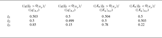
(horizontal motion) yields the following results, given in table 2: for all nominal Rayleigh numbers the mean heat fluxes and kinetic energies corresponding to the positive and negative sub-partitions of
 $\xi _1$
and
 $\xi _2$
are close to 50 % of the Eulerian quantities. In contrast, for
 $\xi _3$
the transport of heat and kinetic energy is largely confined to the positive sub-partition. Therefore, transport along the coherent paths described in the present work, related to the sub-partition
 $\xi _3\gt 0$
, is considerably more efficient than transport strictly along the direction of the mean vertical temperature gradient.
Heat flux and kinetic energy corresponding to the positive and negative subsets of the leading eigenvectors
 $\xi _1$
,
 $\xi _2$
and
 $\xi _3$
, in relation to the Eulerian heat flux and kinetic energy, averaged over all nominal Rayleigh numbers (S1–S7). The standard deviation under varying
 ${\textit{Ra}}$
is less than 3 % of the given mean values. Deviations from unity in the sum of two associated sub-partitions are caused by the spatially coarser Lagrangian sampling of the fields as compared with the Eulerian solution.

(a) Eulerian heat flux,
 $\langle q (\boldsymbol{r},t)\rangle _A (t)$
, (solid curve) compared with the heat flux carried by the tracer particles,
 $\langle q (\boldsymbol{r}^+)| \xi _3 \rangle _{N_p}$
, decomposed into positive and negative
 $\xi _3$
-subsets. (b) Eulerian kinetic energy,
 $\langle E_u (\boldsymbol{r}) \rangle _A (t)$
(solid curve) compared with the kinetic energy carried by the tracer particles,
 $\langle E_u(\boldsymbol{r}^+)| \xi _3 \rangle _{N_p}$
, decomposed into positive and negative
 $\xi _3$
-subsets. The red line in each subfigure represents the error between Eulerian and Lagrangian fields,
 $\epsilon = \langle f (\boldsymbol{r},t)\rangle - \langle f (\boldsymbol{r}^+)| \xi _3 \rangle$
. Data shown for simulation run S7.

4.2. Tracer movement between clusters
With the third eigenvector representing a partition into coherent transport paths and stagnation regions, it is possible to quantify how tracer particles move between the two subsets. This is done by tracking the value
 $\xi _{3}$
of each tracer particle and extracting the lengths of the individual time intervals that it is continuously assigned to the positive transport subset
 $\xi _3\gt 0$
and the negative stagnation subset
 $\xi _3 \lt 0$
, respectively. The PDFs of these individual time intervals accumulated for all tracer particles are shown in figure 8, where the black symbols correspond to the lowest Rayleigh number and the blue symbols to the highest Rayleigh number of the present simulations (S1 and S7, see table 1). All PDFs are characterised by pronounced exponential tails, indicating a high probability of long time intervals spent continuously in the same subset. The tails fall off considerably faster for larger Rayleigh numbers. Thus, the probability of a particle spending longer times in either the transport or stagnation subset is substantially reduced as compared with lower
 ${\textit{Ra}}$
, in agreement with the increased intensity of mixing at larger Reynolds and Rayleigh numbers. The slightly elevated tails of the
 $\xi _3\lt 0$
distributions in comparison with the case of
 $\xi _3\gt 0$
in figure 8 also suggests a tendency that at both
 ${\textit{Ra}}$
particles are more likely to spend longer time intervals in the stagnation subsets. A possible reason could be the significantly reduced magnitude of velocities within the stagnation regions as compared with the transport paths (cf. figures 7
b and 3
a–c).
Probability density function of length of time intervals that Lagrangian tracers spend in the transport cluster
 $\xi _3 \gt 0$
and the stagnation cluster
 $\xi _3 \lt 0$
for
 ${\textit{Ra}} = 1.56 \times 10^{12}$
(S7) and
 ${\textit{Ra}} = 3.98 \times 10^{6}$
(S1).

5. Reduced description of global transport
In order to obtain information about the global structure of advective transport and of the average dynamical imprint of the thermal driving, in the following, a reduced description of the flow based on the coherent transport paths is established. Their global spatial structure is discernible in the velocity field in figure 3(a–c) as well as in the Lagrangian transport cluster in figure 5(d). However, a simpler, yet quantifiable reduced representation appears to be possible. Since a key feature of plume-related transport is the presence of accompanying large-scale vortices (cf. figure 2
b,c), a pertinent approximation of the transport structure is obtained via scale filtering (Germano Reference Germano1992) of the vorticity field. The filter operation written in terms of the Fourier transformed vorticity field,
 $\hat {\omega }(\boldsymbol{k},t)$
, reads
 \begin{equation} \hat {\omega }_{k_{\!f}}(\boldsymbol{k},t) = \hat {G}_{k_{\!f}}(\boldsymbol{k}) \hat {\omega }(\boldsymbol{k},t), \end{equation}
with an isotropic Gaussian filter kernel
 $\hat {G}_{k_{\!f}}(\boldsymbol{k})$
that is defined following Pope (Reference Pope2001, § 13.2.2) as
 \begin{equation} \hat {G}_{k_{\!f}}(\boldsymbol{k}) = \text{exp} \big[-(1/24) |\boldsymbol{k}|^2 (\pi /{k_{\!f}})^2 \big]. \end{equation}
It leads to a smooth decay of Fourier modes around
 ${k_{\!f}}$
and hence to a low-pass-filtered vorticity where mainly the wavenumbers
 $|\boldsymbol{k}| \lt {k_{\!f}}$
are retained. Applying an inverse Fourier transform to
 $\hat {\omega }_{k_{\!f}} (\boldsymbol{k},t)$
yields the coarse-grained representation of the vorticity field in configuration space,
 $\omega _{k_{\!f}} (\boldsymbol{r},t)$
, which lacks the high wavenumber components as determined by the filter kernel. In figure 9(a–c) the field of kinetic energy is shown as an indicator for the transport paths, overlaid with the zero isoline of the scale-filtered vorticity (cyan) at
 ${k_{\!f}} \in \{1,3.5,10\}$
for (a)–(c) respectively. A parameterisation based on the zero isoline of vorticity is obtained by calculating the field
 $d(\boldsymbol{r},\omega _{k_{\!f}}=0)$
, representing the smallest Euclidean distance of each grid point to
 $\omega _{k_{\!f}} = 0$
. Isolines of this distance field, which for brevity is denoted as
 $d_{k_{\!f}}$
in the following, are shown colour coded in figure 9(a–c). The zero-vorticity line and the corresponding distance field vary in shape depending on
 ${k_{\!f}}$
, becoming more complex and convoluted with increasing
 ${k_{\!f}}$
as a larger amount of small-scale fluctuation remains unfiltered. A good approximation of the transport paths via
 $d_{k_{\!f}} = 0$
is obtained for
 ${k_{\!f}} = 3.5$
, while for
 ${k_{\!f}} = 1$
and
 ${k_{\!f}} = 10$
the lines appear under- and over-fitted, respectively. In figure 9(d–f) a
 $2048^2$
section of the same kinetic energy field and zero-vorticity line as in (a–c) is shown, overlaid with the local velocity vectors, showing that the zero line of
 $d_{3.5}$
captures the structure of the coherent transport paths rather accurately. Motivated by this visual impression, a more quantitative approach presented in the following allows us to properly separate the large scales contributing to the transport paths from the smaller-scale fluctuations. Note that a similar distance-field parameterisation has previously been established based on the zero isoline of the large-scale temperature field in wall-bounded, laterally unconfined RBC in order to extract the structure and mean imprint of the LSC (Berghout, Baars & Krug Reference Berghout, Baars and Krug2021; Blass et al. Reference Blass, Verzicco, Lohse, Stevens and Krug2021). There, a spectral gap of reduced energy density is observed between an energy peak related to large-scale convection rolls and an additional increased amount of energy related to small-scale fluctuations. Such a clear scale separation is, however, not found in the present homogeneous system without LSC. Here, the spectrum of the compensated spatial heat flux,
 $\hat {q}(k) k^{9/5}$
, shown in figure 4, exhibits a continuous excitation of large bandwidth without such an obvious separation of large and small scales. Therefore, in the following the determination of the optimal
 ${k_{\!f}}$
is based on the negative spatial correlation of
 $E_u (\boldsymbol{r},t)$
with
 $d_{k_{\!f}} (\boldsymbol{r},t)$
, which is particularly well recognisable in figure 9(b), where on average an increase of
 $d_{k_{\!f}} (\boldsymbol{r})$
corresponds to a decrease in
 $E_u (\boldsymbol{r})$
. Finding the optimally fitted distance field hence amounts to finding the filter wavenumber that maximises the modulus of the correlation
 \begin{equation} C_{E_u,d_{k_{\!f}}} = \frac { \langle E^{\prime}_u(\boldsymbol{r},t) d^{\prime}_{k_{\!f}}(\boldsymbol{r},t) \rangle _{\textit{A}\text{,}\textit{t}} }{\sigma _{E'} \sigma _{d'}}, \end{equation}
under variation of
 ${k_{\!f}}$
. Here, the prime denotes the mean-centred fields,
 $f' = f - \langle f \rangle _{\textit{A}\text{,}\textit{t}}$
. Figure 10(a) shows
 $C_{E_u,d_{k_{\!f}}}$
versus
 ${k_{\!f}}$
for a sequence of filter wavenumbers
 ${k_{\!f}} \in [1,200]$
with step size
 $\Delta {k_{\!f}} = 0.25$
. A negative value is apparent for all filter wavenumbers, meaning that
 $d_{k_{\!f}} (\boldsymbol{r},t)$
is negatively correlated to
 $E_u (\boldsymbol{r},t)$
over the entire range of filter wavenumbers. The diamond, cross and circle indicate the filter wavenumbers
 ${k_{\!f}} \in \{1,3.5,10\}$
of the distance fields shown in figure 9(a–c), respectively. The maximal negative correlation at approximately
 ${k_{\!f}} = 3.5$
implies that filtering at this wavenumber yields the best approximation of the global transport structure in the present system in terms of
 $E_u (\boldsymbol{r})$
. The good agreement of this wavenumber with the wavenumber of the maximum spectral heat transport shown in figure 4(d) corroborates the relation of the reduced transport structure to the plume-condensation scale. The varying structure of the reduced transport paths depending on filter wavenumber is reflected in the PDFs of
 $d_{k_{\!f}}$
in figure 10(b), where the influence of higher wavenumbers leads to heavier tails of the distribution. The PDF corresponding to the optimally fitted distance field at
 ${k_{\!f}}=3.5$
is hence characteristic for the shape of coherent transport paths of the system at the given Rayleigh number.
(a–c) Field of kinetic energy,
 $E_u (\boldsymbol{r}) = |\boldsymbol{u}(\boldsymbol{r})|^2 /2$
, at large
 ${\textit{Ra}}$
(S7), overlaid with contours that represent the Euclidean distance of each grid point from the zero line of the Gauss-filtered vorticity,
 $d(\boldsymbol{r},\omega ^{k_{\!f}}=0)$
, with filter wavenumber
 ${k_{\!f}} \in \{1,3.5,10\}$
in (a–c) respectively; (d–f)
 $2048^2$
section of the same field as indicated in (a–c), overlaid with zero line and local velocity vectors.

(a) Spatial correlation of the field of kinetic energy,
 $E_u(\boldsymbol{r},t)$
, and the field
 $d_{k_{\!f}} (\boldsymbol{r},t)$
at large
 ${\textit{Ra}}$
(S7). The latter represents the Euclidean distance of each point to the zero line of the low-pass-filtered vorticity,
 $\omega _{k_{\!f}} (\boldsymbol{r},t)$
. The green, red and blue markers indicate the filter wavenumber of the distance fields displayed with contours in figure 9(a–c). (b) Probability density function of
 $d_{k_{\!f}} (\boldsymbol{r})$
with
 ${k_{\!f}}$
corresponding to the four markers in figure 10(a).

In figure 11(a) the normalised covariance
 $C_{E_u,d_{k_{\!f}}}$
is shown versus
 ${k_{\!f}}$
for S1–S7, where the black curve corresponds to the data shown in figure 10(a). The filter wavenumber that maximises the modulus of
 $C_{E_u,d_{k_{\!f}}}$
and thus yields the optimally fitted approximation of the transport paths at each
 ${\textit{Ra}}$
is denoted as
 $\tilde {k}$
and shown in figure 11(b). The increase in optimal filter wavenumber
 $\tilde {k}$
shows that from small
 ${\textit{Ra}}$
to large
 ${\textit{Ra}}$
contributions of increasingly smaller scales are contained within the transport paths, a finding that is in agreement with the visual impression from figure 3(a–c). We note that, in a statistially stationary state, the physical characteristics related to the correlation function such as kinetic energy, heat flux, advective transport structure and thermal plumes are all expected to be of maximum amplitude at the largest scales of the flow, due to, e.g. the spectral scaling behaviour of energy and temperature fluctuations. As the dynamically active size of the system is limited from above by the applied large-scale damping (cf. Appendix A), it might be plausible to expect that the transport properties of the turbulent flow discussed in the present work are dominated by the large-scale boundary conditions. However, in § 5.3, we show that the transport structure also exists in an approximately self-similar manner on smaller inertial scales of the flow (for the scale dependence of the scale-adapted correlation function, see figure 16
a). The optimally fitted distance field for each
 ${\textit{Ra}}$
based on
 $\tilde {k}$
is denoted as
 $\tilde {d} (\boldsymbol{r},t)$
in the following. In figure 11(c) the PDF of
 $\tilde {d}(\boldsymbol{r},t)$
is displayed for each simulation. Despite the varying wavenumbers that contribute to
 $\tilde {d} (\boldsymbol{r},t)$
at each
 ${\textit{Ra}}$
these curves overlap, showing that the large-scale coherent paths have statistical characteristics that are essentially independent of
 ${\textit{Ra}}$
.
(a) Same correlation coefficient as in figure 10, for different Rayleigh numbers. (b) Optimal filter wavenumber,
 $\tilde {k}$
, determined as the wavenumber that maximises the modulus of
 $C_{E_u,d_{k_{\!f}}}$
. (c) Probability density function of the optimally fitted distance field
 $\tilde {d}$
at each
 ${\textit{Ra}}$
.

5.1. Anisotropy of reduced transport paths
An important property of the transport paths which can be deduced from
 $\tilde {d}$
is their orientation in space, which indicates the locally dominant direction of advective transport. This orientation is determined by the angle
 $\varphi _y$
of the local tangent at each point on the zero line of
 $\tilde {d}$
with respect to the y-axis, where
 $\{ \varphi _y \in \mathbb{R} \mid 0 \leqslant \varphi \leqslant \pi /2 \}$
. In figure 12(a,b) the zero line of
 $\tilde {d}$
is shown in colours indicating the local angle for two snapshots from the smallest and largest Rayleigh number simulations (see table 1). The grey level sets, corresponding to regions where
 $E_u (\boldsymbol{r}) \gt 0.6 \sigma _{E_u}$
, are shown to emphasise that the dynamical imprint of the thermal driving is mainly confined to the reduced transport paths. Based on the local angle it is possible to decompose the zero line into vertically oriented segments with
 $\varphi _y \lt \pi /4$
(blue segments) and horizontally oriented segments with
 $\varphi _y \gt \pi /4$
(red segments). The PDFs of the lengths
 $s$
of the individual line segments are shown in figure 12(c), separated for vertical and horizontal segments. All PDFs feature exponential tails, with the ones for vertical paths being elevated, underlining the preference of vertical transport due to the anisotropic driving. Interestingly, the PDFs of horizontal transport paths coincide for both
 ${\textit{Ra}}$
while the PDF of vertical transport paths is considerably flatter at small
 ${\textit{Ra}}$
. Thus, the observed increase in isotropy towards large
 ${\textit{Ra}}$
(see figure 3) arises solely due to a breakdown of vertical transport paths, while the transport length along the horizontal direction appears to remain unchanged. This means that at larger
 ${\textit{Ra}}$
thermal plumes travel shorter distances, which can be explained by the stronger material exchange with the turbulent environment observed in figure 8. The ratio of cumulated vertical to cumulated horizontal path length is shown as crosses in figure 12(d) versus
 ${\textit{Ra}}$
. The data points coincide with the ones of the ratio of vertical to horizontal kinetic energy in figure 3(d) which are plotted here again as circles. This is an important finding as it shows that the energetic anisotropy due to the thermal driving is closely reflected within the geometry of the transport paths, stressing their relevance for the description of HRB convection.
(a,b) Reduced transport paths given by zero lines of
 $\tilde {d}$
at smallest and largest
 ${\textit{Ra}}$
, colour coded by angle. The grey regions indicate the threshold
 $E_u \gt 0.6 \sigma _{E_u}$
. (c) Probability density functions of length of horizontal and vertical path segments, for the same
 ${\textit{Ra}}$
values. (d) Ratio of cumulated vertical to horizontal transport path length (plus) and ratio of vertical to horizontal kinetic energy (circles) taken from figure 3(d).

5.2. Mean influence of coherent paths
The approximation of the large-scale transport structure via
 $\tilde {d} (\boldsymbol{r},t)$
offers a self-adjusting reference frame based on the coherent transport paths. Their mean imprint on the field is evaluated in the following by calculating conditional averages of different field quantities binned with respect to the distance field
 \begin{equation} \bar {f} (\tilde {d}) = \langle f\! \mid\! \tilde {d} \rangle _{\textit{A}\text{,}\textit{t}} / \langle f \rangle _{\textit{A}\text{,}\textit{t}}. \end{equation}
5.2.1. Spatial heat flux, velocity and temperature
In figure 13(a–c) the mean profiles of spatial heat flux, velocity magnitude and magnitude of temperature fluctuations with respect to the optimally fitted distance field are shown for each
 ${\textit{Ra}}$
. In general, the profiles of heat flux are the steepest. Thus, heat flux is strongly confined to the transport paths and declines sharply further away. The velocity profiles are slightly flatter, indicating a weaker confinement. For the heat flux and the velocity a weak trend with
 ${\textit{Ra}}$
is observed, where the profiles become slightly steeper with decreasing
 ${\textit{Ra}}$
. This is not surprising as with smaller
 ${\textit{Ra}}$
also the intensity of turbulent fluctuations decreases and hence there is less momentum transport between the transport paths and the adjacent shear layers and large-scale vortical regions. The profile of the temperature magnitude shows a stronger dependence on Rayleigh number. For the smallest
 ${\textit{Ra}}$
it has a similar shape as the velocity profile, suggesting an equally strong confinement of temperature fluctuations to the transport paths, which reflects the strong correlation of
 $\theta$
and
 $u_y$
at small
 ${\textit{Ra}}$
inferred from figure 3(e). With increasing Rayleigh number, however, the temperature profile flattens and approaches an asymptotic linear profile for
 ${\textit{Ra}} \gt 10^9$
. In contrast, the velocity profile
 $\bar {u}(\tilde {d})$
remains comparably stable with increasing
 ${\textit{Ra}}$
. This suggests that the spatial decorrelation of the two fields at large
 ${\textit{Ra}}$
(see figure 3
e) is due to an enhanced turbulent mixing, leading to a reduced confinement of temperature fluctuations to the coherent transport paths.
Conditional average (5.4) of (a) vertical spatial heat flux, (b) magnitude of velocity and (c) magnitude of temperature fluctuations evaluated with respect to the distance field
 $\tilde {d} (\boldsymbol{r})$
for different Rayleigh numbers.

5.2.2. Nonlinear cross-scale flux
From § 3.2 it is evident that the thermal driving has a characteristic influence on the nonlinear fluxes at large scales. To further analyse this influence with respect to the role of coherent transport paths, the fluxes are investigated in configuration space. The required framework is obtained following Germano (Reference Germano1992) and Chen et al. (Reference Chen, Ecke, Eyink, Rivera, Wan and Xiao2006) by applying a low-pass Gaussian filter (equation (5.1)) to each term of the governing equations (2.3)–(2.6) in spectral space. This allows the derivation of evolution equations for the filtered kinetic energy
 $(E_u)_{k_{\!f}} = \boldsymbol{u}_{k_{\!f}}\boldsymbol{\cdot }\boldsymbol{u}_{k_{\!f}} / 2$
, thermal energy
 $(E_{\theta })_{k_{\!f}} = \theta _{k_{\!f}} \theta _{k_{\!f}} /2$
and enstrophy
 $(\varOmega )_{k_{\!f}} = \omega _{k_{\!f}} \omega _{k_{\!f}} /2$
, as
 \begin{align} \partial _t (E_u)_{k_{\!f}} &= - \boldsymbol{\nabla }\boldsymbol{\cdot }\boldsymbol{J}_{\boldsymbol{u}} - 2 \tilde {\nu } \boldsymbol{S}_{k_{\!f}} : \boldsymbol{S}_{k_{\!f}} + \theta _{k_{\!f}} \boldsymbol{u}_{k_{\!f}} \boldsymbol{\cdot }\boldsymbol{e_y} + \boldsymbol{S}_{k_{\!f}} : \boldsymbol{\tau }, \end{align}
 \begin{align} \partial _t (E_{\theta })_{k_{\!f}} &= - \boldsymbol{\nabla }\boldsymbol{\cdot }\boldsymbol{J}_{\theta } - \tilde {\kappa } (\boldsymbol{\nabla }\theta _{k_{\!f}})^2 + \theta _{k_{\!f}} \boldsymbol{u}_{k_{\!f}} \boldsymbol{\cdot }\boldsymbol{e_y} + \boldsymbol{\nabla }\theta _{k_{\!f}} \boldsymbol{\cdot }\boldsymbol{\vartheta }, \end{align}
 \begin{align} \partial _t (\varOmega )_{k_{\!f}} &= - \boldsymbol{\nabla }\boldsymbol{\cdot }\boldsymbol{J}_{\omega } - \tilde {\nu } (\boldsymbol{\nabla }\omega _{k_{\!f}})^2 + \omega _{k_{\!f}} \partial _x \theta _{k_{\!f}} + \boldsymbol{\nabla }\omega _{k_{\!f}} \boldsymbol{\cdot }\boldsymbol{\sigma}, \end{align}
where
 $\boldsymbol{S}_{k_{\!f}} = 1/2 (\boldsymbol{\nabla }\boldsymbol{u}_{k_{\!f}} + (\boldsymbol{\nabla }\boldsymbol{u}_{k_{\!f}})^T )$
is the rate-of-strain tensor of the remaining large scales,
 $\boldsymbol{\tau } = (\boldsymbol{u}\boldsymbol{u})_{k_{\!f}} - \boldsymbol{u}_{k_{\!f}}\boldsymbol{u}_{k_{\!f}}$
is the small-scale turbulent stress tensor,
 $\boldsymbol{\vartheta } = (\boldsymbol{u} \theta )_{k_{\!f}} - \boldsymbol{u}_{k_{\!f}} \theta _{k_{\!f}}$
is the small-scale turbulent temperature transport and
 $\boldsymbol{\sigma } = (\boldsymbol{u} \omega )_{k_{\!f}} - \boldsymbol{u}_{k_{\!f}} \boldsymbol{\omega }_{k_{\!f}}$
the small-scale turbulent vorticity transport. In the above equations the first terms on the right-hand sides are conservative, representing a redistribution of energy and enstrophy on the resolved scales. The second and third terms are the dissipation and source terms, respectively. Finally, the last terms on the right-hand sides stand for the spatial cross-scale fluxes that represent the nonlinear energy exchange between the remaining large scales
 $k \lt {k_{\!f}}$
and the small scales that have been depleted by the filter operation,
 $k\gt {k_{\!f}}$
. They correspond to an interaction of large-scale gradients with the small-scale turbulent field. Adopting the definition of the flux terms from Rivera et al. (Reference Rivera, Daniel, Chen and Ecke2003) as
 \begin{align} \varPi _{k_{\!f}}^u (\boldsymbol{r},t) &\equiv -\boldsymbol{S}_{k_{\!f}} : \boldsymbol{\tau }, \end{align}
 \begin{align} \varPi _{k_{\!f}}^{\theta } (\boldsymbol{r},t) &\equiv - \boldsymbol{\nabla }\theta _{k_{\!f}} \boldsymbol{\cdot }\boldsymbol{\vartheta }, \end{align}
 \begin{align} \varPi _{k_{\!f}}^{\omega } (\boldsymbol{r},t) &\equiv - \boldsymbol{\nabla }\omega _{k_{\!f}} \boldsymbol{\cdot }\boldsymbol{\sigma }, \end{align}
a positive value represents a direct flux from larger to smaller scales and a negative value stands for an inverse flux from smaller to larger scales. Integrating (5.8)–(5.10) over space and time for a given
 ${k_{\!f}}$
yields the mean nonlinear flux over that wavenumber, which is equivalent to the fluxes in Fourier space, (3.1)–(3.3), as illustrated in figure 14(a–c). The differences between the flux functions in Fourier and configuration space in this figure are caused by the lack of spectral sharpness of the Gaussian filter. A perfect overlap can be achieved by using a sharp spectral cutoff instead of a Gaussian filter, which is, however, not used here due to its lack of locality in configuration space. Since the dynamical influence of the transport structure and the underlying thermal plumes is dominant around the condensation scale
 $k = 3{-}4$
(cf. heat flux spectrum in figure 4
d), the local flux fields are investigated for
 ${k_{\!f}} = 3.5$
. They are shown in figure 14(d–f), overlaid with velocity streamlines and the reduced transport paths given by
 $\tilde {d} = 0$
. Locally, both positive and negative fluxes are present, similar to previous results on two-dimensional homogeneous Navier–Stokes turbulence (Chen et al. Reference Chen, Ecke, Eyink, Rivera, Wan and Xiao2006; Xiao et al. Reference Xiao, Wan, Chen and Eyink2009; Wang et al. Reference Wang, Sesterhenn and Müller2023). It appears that large magnitude enstrophy and kinetic energy fluxes are preferentially located on the reduced transport paths while the thermal energy flux exhibits large magnitudes also in the adjacent shear layers.
(a–c) Spatio-temporal average of the filtered cross-scale flux terms
 $\varPi _{k_{\!f}}^{\omega }$
,
 $\varPi _{k_{\!f}}^u$
and
 $\varPi _{k_{\!f}}^{\theta }$
depending on filter wavenumber
 ${k_{\!f}}$
for simulation run S7. For comparison their Fourier-space equivalent ((3.1)–(3.3)) is shown as dashed curves. (d–f) Instantaneous field of cross-scale flux of enstrophy, kinetic energy and thermal energy over
 ${k_{\!f}} = 3.5$
for S7. The large-scale transport grid given by the zero line of
 $\tilde {d}$
and velocity streamlines are indicated by the magenta and green lines, respectively.

The average footprint of the transport grid on the nonlinear fluxes is quantified by their conditional averages (equation (5.4)) with respect to
 $\tilde {d}$
, shown in figure 15(a) for the flux over
 ${k_{\!f}}=3.5$
(black) and the flux over
 ${k_{\!f}}=20$
(grey), where
 ${k_{\!f}}=20$
lies in the inertial range. The mean kinetic energy flux over
 ${k_{\!f}}=3.5$
is negative for all
 $\tilde {d}$
and its magnitude decreases with increasing
 $\tilde {d}$
. The most active region of large-scale inverse kinetic energy flux is therefore close to the transport paths, which comes to no surprise as most of the kinetic energy is confined there. The thermal energy flux over
 ${k_{\!f}}=3.5$
is positive at all distances to the transport paths. It is large close to
 $\tilde {d} = 0$
and features a maximum at
 $\tilde {d} \approx 0.75$
, followed by a decline for increasing distance. The maximum can be related to the increased transport of temperature fluctuations away from the transport paths at large
 ${\textit{Ra}}$
, as put forward in figure 13(c), which also enhances the nonlinear flux in the further vicinity of the transport paths. Importantly, for inertial scales
 ${k_{\!f}}=20$
, the conditioned kinetic and thermal energy fluxes remain qualitatively similar. This is not the case for the conditioned enstrophy flux. For inertial scales at
 ${k_{\!f}}=20$
it is positive at all distances, with decreasing magnitude for increasing
 $\tilde {d}$
. At
 ${k_{\!f}} = 3.5$
however, despite the global negative flux over that wavenumber (see figure 14
a), the enstrophy flux is positive on the transport paths and changes sign at
 $\tilde {d} \approx 0.48 \sigma _{\tilde {d}}$
, featuring a maximum of negative flux at
 $\tilde {d} \approx 1.1 \sigma _{\tilde {d}}$
. This shows that the global negative (inverse) enstrophy flux at large scales has a distinct spatial quality with respect to the large-scale transport structure and the underlying plume motion. The distance threshold corresponding to a positive flux marked in cyan in figure 15(a) is illustrated within the field in figure 15(d) on top of
 $E_u$
and the reduced transport paths. The visual impression is that the inverse flux of enstrophy predominantly emerges with spatial distance to the transport paths in the surrounding shear layers and vortices. This suggests that the inversion is a result of the nonlinear interaction of plumes and the adjacent fluid on large spatial scales.
(a) Conditional average of the spatially resolved nonlinear fluxes of enstrophy, kinetic energy and thermal energy with respect to the distance field
 $\tilde {d}(\boldsymbol{r})$
for simulation run S7. The black and grey lines correspond to the conditioned flux over
 ${k_{\!f}}=3.5$
and
 ${k_{\!f}}=20$
, respectively. (b) Local kinetic energy and reduced transport paths together with the distance threshold of conditionally mean positive enstrophy transfer for S7.

5.3. Inertial-range transport grid
In classical RBC, the scale of global transport is determined by the integral size of the domain, while the scale of thermal plumes is determined by the thickness of the thermal boundary layer (Krishnamurti & Howard Reference Krishnamurti and Howard1981; Zocchi et al. Reference Zocchi, Moses and Libchaber1990; Parodi et al. Reference Parodi, von Hardenberg, Passoni, Provenzale and Spiegel2004). What results is a structure of transport that is decidedly non-universal, most prominently seen in a spectral gap of reduced energy density between large and small scales of the flow (Hartlep et al. (Reference Hartlep, Tilgner and Busse2003), Stevens et al. (Reference Stevens, Blass, Zhu, Verzicco and Lohse2018), Krug, Lohse & Stevens (Reference Krug, Lohse and Stevens2020), see also introduction to § 5). In HRB convection at sufficiently large
 ${\textit{Ra}}$
, due to the lack of boundary layers, no such clear scale separation exists, allowing for the possibility that the spatial structure of transport in the present system exhibits scale-invariant characteristics. To explore the structure of transport on varying scales, the high-pass-filtered velocity field is defined in Fourier space as
 \begin{equation} \hat {\boldsymbol{u}}_{k_h}(\boldsymbol{k},t) = \hat {G}_{k_h}(\boldsymbol{k}) \hat {\boldsymbol{u}}(\boldsymbol{k},t), \end{equation}
where
 $\hat {G}_{k_h}$
is a sharp spectral filter that annihilates all fluctuations at wavenumbers
 $|\boldsymbol{k}| \leqslant {k_{\!f}}$
, while having no effect on the larger wavenumbers. Defining
 $k_h \in [1,600], k_h \in \mathbb{N}$
and applying an inverse Fourier transform on
 $\hat {\boldsymbol{u}}_{k_h} (\boldsymbol{k})$
results in spatial fields with successively decreasing maximal spatial scale, as illustrated on the kinetic energy of the full and two high-pass fields in figure 16(b–d). Similarly to the unfiltered velocity field, the main transport paths of the small-scale fields are approximated by the zero isoline of the Gauss-filtered vorticity,
 $\omega _{{k_{\!f}},k_h} (\boldsymbol{r}) = 0$
, obtained via a shifted Gaussian filter given by
 \begin{equation} \hat {G}_{{k_{\!f}},k_h}(\boldsymbol{k}) = \text{exp}\big[-1/24(|\boldsymbol{k}|-k_h)^2 (\pi / {k_{\!f}})^2\big]. \end{equation}
(a) Maximal correlation of high-pass kinetic energy field
 $(E_u)_{k_h}$
and optimally fitted distance field
 $\tilde {d}_{k_h}$
depending on high-pass wavenumber for run S7. (b–d) Full kinetic energy and high-pass-filtered kinetic energy at two filter wavenumbers for run S7. (e–g) Zero line of optimally fitted distance field, representing the main transport paths of the fields in the top row.

This filter leads to a smooth decay of Fourier modes with
 $k \gt k_h$
and therefore acts on the high-pass-filtered fields similarly to the Gaussian filter defined by equation (5.2) for the full fields. Similar to the approach described above, the zero lines shown in figure 16(e–g) that optimally represent the transport paths are determined based on the maximum modulus of the correlation given by (5.3) under variation of
 ${k_{\!f}}$
. However, the correlation depending on
 ${k_{\!f}}$
is not computed for the full field
 $E_u (\boldsymbol{r})$
and distance field
 $d(\boldsymbol{r},\omega _{k_{\!f}}=0)$
, but instead for the high-pass-filtered kinetic energy
 $(E_u)_{k_h} (\boldsymbol{r}) = (\boldsymbol{u})_{k_h} \boldsymbol{\cdot }(\boldsymbol{u})_{k_h} / 2$
and distance field
 $d(\boldsymbol{r},\omega _{{k_{\!f}},k_h}=0)$
.
The quality of the transport structure approximation by the optimally fitted distance field
 $\tilde {d}_{k_h}$
is determined for each high-pass velocity field by consideration of the correlation
 $C_{(E_u)_{k_h},\tilde {d}_{k_h}}$
versus
 $k_h$
, as shown in figure 16(a). For small
 $k_h$
, the maximal absolute correlation is
 $C \approx -0.45$
, agreeing with that of the full fields,
 $E_u (\boldsymbol{r})$
and
 $\tilde {d} (\boldsymbol{r})$
, as shown in figure 10. Increasing the high-pass wavenumber,
 $k_h$
, to inertial-range wavenumbers leads to a decrease of absolute correlation, to a value of
 $C \approx -0.3$
, followed by an approximate plateau for
 $6 \leqslant k_h \leqslant 200$
. At dissipative scales,
 $k_h \gt 200$
, a further decrease of absolute correlation is observed. These results reflect that the advective transport structure expressed via
 $\tilde {d}$
is asymptotically self-similar on inertial scales (approximately constant correlation with
 $(E_u)_{k_h}$
). The overall decrease of the correlation modulus for growing
 $k_h\gt 0$
is the expected consequence of the loss of information inflicted by the filter operation.
Potentially scale-invariant characteristics of advective transport are investigated in the following, where the reduced transport structure is analysed depending on
 $k_h$
. To this end, the PDF of
 $\tilde {d}_{k_h}$
at different
 $k_h$
is shown in figure 17(a) together with the PDF of the distance field
 $\tilde {d}$
representing the large-scale transport paths. The curves show good agreement for all
 $k_h$
, suggesting that the spatial properties of dominant transport paths exhibit a rather good level of scale invariance. An important difference between the large- and inertial-scale transport structure is, however, present in terms of the anisotropy of coherent transport paths. This is shown in figure 17(b), where the ratio of cumulated vertical to horizontal transport length (see § 5.1 for methodology) is illustrated depending on
 $k_h$
. At large scales this ratio is distinctly above 1, indicating that the length of vertical transport paths is considerably longer than that of horizontal paths, which reflects the large-scale anisotropy of the system that was observed earlier. With increasing
 $k_h$
this anisotropy, however, decreases, reaching a constant value around 1.06 for
 $k_h \gt 4$
. As expected, the anisotropy due to the thermal driving is therefore mainly observable on the largest scales of the flow, while the inertial and dissipative ranges exhibit nearly isotropic behaviour.
(a) Probability density function of the optimally fitted distance field representing the integral transport structure (
 $\tilde {d}$
) and the transport structure of high-pass fields at the respective
 $k_h$
(
 $\tilde {d}_{k_h}$
) for run S7. (b) Ratio of vertical and horizontal transport paths versus
 $k_h$
.

6. Summary and conclusion
The present investigation explores the spatial structure of advective transport in direct numerical simulations of turbulent mean-gradient-driven two-dimensional, homogeneous Boussinesq convection with periodic boundaries, also denoted as HRB convection, over a range of Rayleigh numbers (
 ${\textit{Ra}}$
) from
 $\textit {Ra} \simeq 10^6$
to
 $\textit {Ra} \simeq 10^{12}$
. The absence of solid boundaries leads to a flow structure that is fundamentally different from wall-bounded RBC. In the wall-bounded case, thermal plumes are embedded in a LSC, which governs advective transport (Zocchi et al. Reference Zocchi, Moses and Libchaber1990; Kadanoff Reference Kadanoff2001; Xia et al. Reference Xia, Sun and Zhou2003; Shishkina & Wagner Reference Shishkina and Wagner2007). The present study shows that, instead of such a dominant large-scale structure induced by buoyant drive and boundaries, in two-dimensional statistically homogeneous convection a detectable large-scale anisotropy of the flow along the vertical direction exists. The anisotropy reflects the buoyant driving of the system and diminishes with increasing nominal Rayleigh number due to increasing intensity of turbulent motion. Furthermore, turbulent HRB convection is dynamically dominated by the localised emergence and condensation of thermal plumes. It is found that their propagation and nonlinear interaction determine the large-scale energetic and structural characteristics of the system. Most importantly, the homogeneous flow exhibits spatio-temporally coherent paths that permeate the entire system and establish a transport structure characterised by localised mean velocities. While these paths are present at all considered Rayleigh numbers, the associated transport characteristics undergo a transition from highly anisotropic at small Ra to nearly isotropic at large Ra. This transition is not due to a varying effective injection of energy but caused by a decorrelation of vertical velocity and temperature as a result of an increasingly turbulent flow. Via an analysis of the scale-dependent contributions to the energy and enstrophy budgets, it is furthermore found that the large-scale coherent paths exhibit a distinct spectral footprint, with a maximum in the heat flux spectrum and an accompanying inversion of the large-scale enstrophy flux. A cluster analysis of Lagrangian tracer trajectories based on their kinematic dissimilarity is performed that yields a reduced representation of the flow and allows us to extract its main transport characteristics. A statistically stable hierarchy on distinct, large-scale kinematic properties is identified: the most distinctive dynamical feature corresponds to opposing vertical motion due to the buoyant acceleration of fluid particles, while the second most dominant characteristic is linked to opposing motion along the horizontal direction that arises due to nonlinear feedback on the vertical motions in the flow. Both horizontal and vertical transport clusters comprise two non-overlapping sub-partitions that contribute close to 50 % of the respective transport (heat flux and kinetic energy) each. Most importantly, the third cluster resembles the coherent transport structure, indicating the near isotropy of advective transport at high Ra and its dominance with respect to spatial heat flux and kinetic energy, to which the structure contributes approximately
 $80\,\%$
. Thus, in two-dimensional convective turbulence at all nominal Rayleigh numbers considered in the present paper (
 $\sim\! 10^6$
–
 $10^{12}$
), the identified transport structure gives rise to more efficient advective transport than flow components oriented strictly along the direction of the mean temperature gradient.
The above-mentioned transport structure allows for a reduced representation of the flow that facilitates the analysis of its transport properties. The reduction is achieved by an appropriate scale filtering of the vorticity, yielding a projection of transport paths onto the zero isoline
 $\omega _{k_{\!f}} = 0$
of the scale-filtered vorticity field. We show that the overall shape of the transport paths is almost independent of Ra. An analysis of individual vertical and horizontal line segments indicates that the decrease of energetic anisotropy with Ra is reflected in a reduction of vertical transport length, while the horizontal transport length remains statistically stable. Mean profiles with respect to the transport paths agree with an underlying decorrelation of vertical velocity and temperature due to an enhanced transport of temperature fluctuations away from the paths and into adjacent shear layers and vortical regions. Mean profiles of local nonlinear fluxes resolved in configuration space furthermore indicate that the inversion of the enstrophy flux observed at large scales is caused within the regions next to and in between the transport paths. It is therefore a characteristic feature of the thermal driving and the resulting global transport structure. Approximate scale invariance of the transport structure in the turbulent inertial range is observed as well by employing successive spectral cutoff filtering. In addition and despite a change of the anisotropy level between large- and inertial-scale transport, the overall structure of paths appears to be statistically independent of Ra.
Acknowledgements
The authors thank J.-M. Teissier for fruitful discussions. Computing resources from the Max Planck Computing and Data Facility (MPCDF) are also acknowledged.
Funding
This work was supported by the German Research Foundation (DFG) within the Research Training Group GRK 2433.
Declaration of interests
The authors report no conflicts of interest.
Appendix A. Tests and evaluation of the large-scale energy sink
In the following, the results of numerical tests are discussed to evaluate the effects of the large-scale damping on the investigated class of flow. The specific choice of the damping coefficients
 $\beta _u = \beta _{\theta } = 3$
(see (2.3) and (2.4)) is outlined as well. For the sake of conciseness, in this appendix both coefficients are represented by a single parameter
 $\beta$
as they are set to identical values throughout the present work.
The scales of length and time that characterise the large-scale damping are estimated exemplarily by use of the relevant terms of the momentum equation in Fourier space. For the temperature fluctuations the reasoning is similar. The relevant equation reads
 \begin{equation} \partial _t \hat {\boldsymbol{u}} (\boldsymbol{k},t) = - \beta k^{-2} \hat {\boldsymbol{u}} (\boldsymbol{k},t). \end{equation}
A solution of this equation is
 \begin{equation} \hat {\boldsymbol{u}} (\boldsymbol{k},t) = \hat {\boldsymbol{u}} (\boldsymbol{k},0) e^{-\beta k^{-2}t}. \end{equation}
Thus, the damping acts on fluctuations at wavenumber
 $k$
on a time scale given by order of magnitude as
 $\tau \sim k^2/\beta$
. In the present BO regime of the flow under consideration, the damping becomes important around
 $\tau \simeq 1$
, as the time is given in units of the large-scale buoyancy time. This yields an order-of-magnitude estimate for the wavenumber characterising the upper limit of the spectral interval directly affected by the damping term as
 $k^* \sim \sqrt \beta$
. Therefore, the dynamics of Fourier modes at wavenumbers
 $k \lesssim k^*$
tends to be dominated by the damping such that they can be considered as dynamically suppressed. Based on this estimate and a set of test simulations (see below), the value of
 $\beta =3$
is chosen for the production simulations, as this value damps the most unstable elevator mode corresponding to
 $(k_x,k_y)= (1,0)$
(cf. § 2) sufficiently, while exerting an influence on Fourier modes at larger
 $k$
that the authors regard as tolerably small.
These considerations are substantiated by a series of test simulations based on the configuration of run S6 under variation of
 $\beta$
between 0.3 and 90. Figure 18(a,b) shows the spectra of heat flux,
 $\hat {q}(k)$
, and nonlinear cross-scale enstrophy flux,
 $\hat {\varPi }_{\omega }$
, for varying damping magnitudes
 $\beta$
. The black curve in each subfigure represents the fiducial simulation with
 $\beta = 3$
. In agreement with the reasoning given above, the largest-scale modes at the Fourier shell
 $k=1$
are dominating
 $\hat {q}(k)$
for
 $\beta =0.3$
, reflecting the dynamical effect of the mechanism driving the elevator instability. This instability has a strong influence on the PDFs of
 $q_y$
and
 $\theta$
shown in figure 18(c,d), where the resulting large-magnitude fluctuations lead to pronounced tails. These tails diminish for
 $\beta \gtrsim 1$
, showing that the elevator mode indeed becomes dynamically suppressed. The spectra and PDFs indicate that in this case all simulations exhibit a finite level of similarity. The key spectral characteristics used for the analysis in the present work, such as the large-scale peak in
 $\hat {q}$
and the inversion of
 $\hat {\varPi }_{\omega }$
from negative to positive values, remain qualitatively similar, albeit shifted to larger
 $k$
for higher
 $\beta$
. This shift, determined by the smallest dynamically active wavenumber
 $k_{\textit{min}} (\beta ) \simeq \max (1,\sqrt \beta )$
, is indicated by the linear markers in figure 18(a) and represents an upper bound for the emergence of large-scale structures at a given
 $\beta$
. The damping coefficients can thus be interpreted as parameterising the finite size of the system. This also influences the characteristic scale of elevator solutions as those are most unstable at lowest spatial wavenumbers along the direction of gravity.
(a,b) Compensated shell spectra of effective energy injection rate and nonlinear cross-scale flux of enstrophy for different damping coefficients
 $\beta$
. The estimate of the smallest dynamically active wavenumber,
 $k_{\textit{min}} (\beta ) \simeq \max (1,\sqrt \beta )$
, is indicated by linear markers. (c,d) Probability density functions of effective energy injection rate and temperature fluctuations for different damping magnitudes.

The large-scale energetic anisotropy of the system, shown in figure 19(a), is another important diagnostic in the present work. It displays an approximate plateau around 1.35 for
 $1 \lesssim \beta \lesssim 30$
. This indicates an additional structural similarity in this range of damping coefficients. The substantial deviation from the plateau value for
 $\beta =0.3$
underlines the strong influence of the elevator mode. Figure 19(a) also shows that, aside from insufficient damping, an excessive damping alters the large-scale anisotropy, as seen by the increase towards 1.5 for
 $\beta = 90$
. The moderate increase in anisotropy relative to the plateau value is the result of the shift of
 $k_{\textit{min}}$
towards the dissipative spectral fall off that leads to a significant reduction of small-scale turbulent fluctuations (see figure 18
a). This indicates that for
 $\beta \gt 30$
the damping has a considerable influence on the small scales of the flow. The structural similarity in the range
 $1 \lesssim \beta \lesssim 30$
is not restricted to the large energetically dominant scales of the flow but it also appears if the anisotropy is analysed in a scale-dependent manner by computing vertical and horizontal kinetic energies with the help of scale-dependent second-order longitudinal velocity increments
 \begin{equation} (\delta u_{\parallel }( \boldsymbol{l} ))^2 = \left ((\boldsymbol{u} (\boldsymbol{r}+\boldsymbol{l}) - \boldsymbol{u} (\boldsymbol{r}) ) \boldsymbol{\cdot }\frac {\boldsymbol{l}}{l } \right )^2, \end{equation}
and restricting
 $\boldsymbol{l}$
to either
 $\boldsymbol{l}_x = \pm (l,0)^T$
or
 $\boldsymbol{l}_y = \pm (0, l)^T$
. With this diagnostic, the mean kinetic energy of fluctuations in vertical and horizontal direction at wavenumber
 $k$
is captured by sampling a large number (N = 10 000) of increments at separations
 $l \sim \pi /k$
. By varying k such that
 $\{ k \in \mathbb{N} \mid 1 \leqslant k/k_{\textit{min}} \leqslant 100 \}$
the corresponding sequence of spatial increments starts at the respective largest dynamically active spatial scale at the given
 $\beta$
and progresses to smaller scales. The resulting anisotropy that depends on
 $k/k_{\textit{min}}$
for different damping magnitudes is shown in figure 19(b), showing that the decrease of anisotropy from the largest dynamically active wavenumber to smaller scales is similar for
 $1 \lesssim \beta \lesssim 30$
.
(a) Ratio of mean vertical and horizontal kinetic energy versus damping coefficient
 $\beta$
. (b) Ratio of vertical and horizontal second-order longitudinal velocity increments versus wavenumber and for varying damping coefficients. The abscissa is normalised by
 $k_{\textit{min}} (\beta ) = \max (1,\sqrt \beta )$
.

Thus, the spectral and structural characteristics of the flow that are of importance for the present work appear to be sufficiently insensitive to a variation in damping magnitude in the interval
 $1 \leqslant \beta \leqslant 30$
. This interval of similarity is bounded by the emergence of the elevator instability at the lower limit and by the suppression of smaller-scale fluctuations at the higher limit of the damping parameter. This strongly suggests that the results of the present work obtained for
 $\beta = 3$
display an acceptable invariance under a variation of the damping parameter within the above interval.