Over the last century and a half, aggregate economic activity in Spain experienced a 43-fold increase, growing at 2.5 percent per year, and per capita GDP was 16 times larger than in 1850, implying an annual rate of 1.9 percent.Footnote 1 GDP per hour worked expanded at a faster rate (2.1 percent) as hours of work per person declined. This economic growth, however, did not take place at a steady rate. During the Golden Age (1950-1974), per capita GDP rose seven times faster than in the previous hundred years, and twice as fast as during the last quarter of the twentieth century. Does factor accumulation or productivity improvement—“abstention” or “ingenuity” to use D. N. McCloskey's words—account for it?Footnote 2 In fact, no consensus has emerged about the relative importance of the contributions of factor accumulation and TFP to GDP growth, nor do we know whether a temporal sequence can be established for their relative contributions to growth.Footnote 3 Susan Collins and Barry Bosworth have suggested that, in its early stages, growth is primarily associated with capital accumulation, while TFP only emerges later.Footnote 4 Studying the sources of Spain's growth over 150 years provides an unusual opportunity to explore these issues.Footnote 5
We use a growth accounting approach which allows us to decompose Spain's long-run growth into the contribution of production factors in terms of quantity and efficiency.Footnote 6 The sources of Spain's growth have changed dramatically since 1850. Broad capital accumulation and TFP growth appear complementary in Spain's long-term growth, and our results for Spain confirm Collins and Bosworth's finding of low TFP growth for countries in their early stages of development.Footnote 7 Factor accumulation dominated long-run growth up to 1950, while efficiency gains led thereafter and, especially, during periods of growth acceleration. The main spurts in TFP and capital correspond to the impact of the railroad (1850s-1880s), the electrification (the 1920s and 1950s), and the adoption of new vintage technology during the Golden Age (1950-1974).
The rest of the article is divided into three parts. We begin by describing the growth accounting adopted in this article and also present our new database, which comprises new estimates of GDP and of capital and labor inputs, over one-and-a-half centuries. We next discuss the role of TFP and factor accumulation in GDP and labor productivity growth. We conclude with some remarks on the significance of the Spanish experience and some questions for future research.
THE “PROXIMATE” SOURCES OF GROWTH: METHODS AND SOURCES
Growth accounting is “a means of allocating observed output growth between the contributions of changes in factor inputs and a residual, total factor productivity, which measures a combination of changes in efficiency in the use of those inputs and changes in technology.”Footnote 8 In the growth accounting approach favored by Dale J. Jorgenson, superlative indices are used, as well as heterogeneous measures of factor inputs that make it possible to separate their contribution to growth into quantity and composition changes.Footnote 9
The Translog Index of Total Factor Productivity
The point of departure for our estimate of the sources of long-run growth in Spain is the production function given by

In which output (Q) is as function of land (X), capital (K), and labor (L) inputs. Specifically,

If we consider two discrete periods of time, we have, after differentiating and taking logarithms,

Here θi denotes the elasticity of output with respect to each input.Footnote 10 Under the assumptions of perfect competition and constant returns to scale these elasticities are equivalent to the share of inputs in total factor payments. Under constant returns to scale, the values of factor shares sum to unity. Weights are then given by the average share of each factor input in total output for the two periods. The translog index of TFP (TFPt-1,t) is the difference between the growth rate of output and a weighted average of the growth rates of factor inputs.
The rate of growth of output and of each input i between two periods is a weighted average of the growth rates of its n quality classes.Footnote 11 The respective equations for output, land, capital, and labor are




where share values are computed as

Capital Input
We develop our measure of capital input (which is an index number of the flow of services provided by the stock of capital) in three successive phases.Footnote 12 First, we construct the stock of capital.Footnote 13 Second, we estimate the rental price of capital (or price of capital services) and the total returns to capital (the value of capital services). Finally, we weight the quantity of each asset by its share in the total returns to capital in order to derive a single capital input index.
Since new additions to the stock of capital (investment, It) are directly observable while the stock, Ct, is not, we need to infer the stock of capital (C) for the year t from the accumulation of investment (I) in past years, taking into account that a part of the stock is retired when obsolete.Footnote 14 With the perpetual inventory method (PIM), the stock of capital in the year t (Ct) is equal to the weighted sum of the investment realized during this same year and the previous ones, where each generation of capital is weighted by its depreciation rate in period t.Footnote 15

Thus the capital stock C in year t is equal to the amount of capital in year t-1 multiplied by 1 minus the depreciation rate (δ) of the year t, plus the gross fixed capital formation, I, during the year t.Footnote 16 The depreciation rate is inversely related to the asset life, so δ = X/T, where X is a parameter (declining balance) and T is the life of each type of asset.Footnote 17 This method generates a measure of capital that takes into account the productive capacity of each component and, hence, measures capital stock in efficiency units.Footnote 18 Since assets lives tend to shorten as one gets closer to the present, three different epochs (1850-1919, 1920-1959, and 1960-2000), with their particular asset lives, are considered for “productive” capital (that is, for all capital assets except residential dwellings).Footnote 19
The second step in developing measures of capital input is to construct rental prices for each type of capital asset. In competitive equilibrium, the cost of producing a unit of capital is equal to its price and the expected rent during its life. If we assume that old and new vintages of capital are perfect substitutes, the rental price of capital, pk, in year t, can be estimated as

where pi is the investment price of the capital good i, r is the nominal rate of return, and δ is the depreciation rate for the capital good i.Footnote 20 The rental price of capital asset i is thus the sum of return per unit of capital, Pit-1 rt, depreciation, δ pit, and the negative of revaluation, [pit - pit-1].Footnote 21
Multiplying the rental price of capital asset i by the quantity of capital stock i, we obtain the returns to capital asset i. Adding up the returns to each type of asset we derive the total returns to capital, which equals capital property compensation. The shares of each type of asset in total returns to capital will be used as weights in the computation of the capital input index. A capital good with a higher amortization rate receives a larger weight in the index of capital input; a million dollars worth of machinery, for example, is allocated a higher weight than a million dollars worth of dwellings. The implication is that changes in the stock composition from long duration (and low rate of return) to short duration (and high rate of return) capital goods represent an increase in the quality of capital. The final step is to construct a capital input index by combining the quantity of each asset with its share in the total returns to capital as in expression 6.
The ratio between the capital input and the capital stock provides a measure of the capital's composition changes or “quality” of capital. However, the idea that technological change embodied in capital is captured by increases in the “quality” of capital lacks consensus and has been rejected by Alwyn Young and Moses Abramovitz and Paul David, who consider that technological progress embodied in capital will appear in the “residual.”Footnote 22
An additional difficulty involved establishing the initial level of capital stock (C0) for each type of asset j in our PIM estimate. We derived this initial stock by assuming that the growth rate of investment during the 1850s was representative of the growth rate of investment prior to 1850.Footnote 23 Algebraically,

where C is the capital stock, I the investment rate, δ the depreciation rate, and g the rate of growth between 1850-1854 and 1855-1859 for each type of asset j. However, it seems plausible that the growth of investment was significantly slower before the 1850s (the decade in which railroads were introduced in Spain) and we have consequently assumed that the initial capital stock would have been twice as high as the figure derived from this computation.Footnote 24
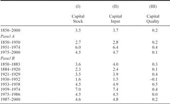
CAPITAL STOCK AND INPUT GROWTH, 1850-2000 (annual average logarithmic rates in percent)

Note:
The long periods in Panel A derive from structural breaks in a trend stationary GDP. Phases in Panel B are obtained as deviations from the trend in GDP (Prados de la Escosura, “Growth”). Growth rates are average annual logarithmic rates of change over periods delimited by peak years.
Sources:
See the text and Prados de la Escosura and Rosés, “Capital Accumulation.”
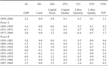
Finally, the long-run interest rate was used to approximate the rate of return on capital under perfect competition.Footnote 25Table 1 presents the evolution of capital stock and input from 1850 to 2000.Footnote 26
As Table 1, Panel A, shows, the capital input and stock do not follow a steady path. Expansion was more intense during the Golden Age, but did not return to the pre-1950 path of growth thereafter. Different phases of growth can be distinguished that, with the exception of the decade of transition to democracy (1975-1985), match GDP performance (Table 1, Panel B). After an initial period of intense progress up to the early 1880s, capital growth slowed down until World War I, resumed in the 1920s, and
THE COMPOSITION OF CAPITAL STOCK, 1850-2000 (1995 pesetas) (percent)

was interrupted from the 1930s to the early 1950s. Since the early 1950s capital accumulation grew at a faster and steadier pace, with a big spurt in the years 1959-1974.
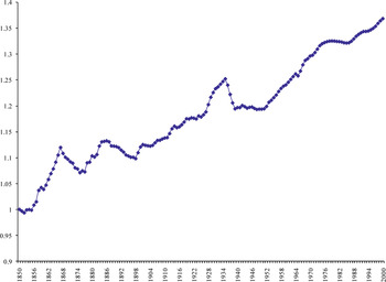
Changes in the composition of capital from residential construction toward nonresidential structures and, especially, machinery and equipment (Figure 1) increased the services provided by the capital stock and reflected a growing gap between the growth rates of capital input and stock (the so-called quality of capital) that rose in phases of fast capital growth (Table 1, column 3 and Figure 2). Three periods stand out in which capital quality grew more rapidly than the long-run trend: from the mid-1850s to the early 1880s, when foreign capital was invested in the railroads construction and in mining; the 1920s, when a new wave of foreign capital inflow and the electrification of Spanish economy took place; and the Golden Age (1953-1974), in which Spain completed electrification and replaced the old vintage capital after two decades of international isolation during the Great Depression, the Civil War (1936-1939), and the early Franco regime. It is worth noting that in spite of receiving a large influx of foreign capital since its accession to the European Union (1986), the “quality” of capital did not rise above the
QUALITY OF CAPITAL, 1850-2000 (1850 = 1)

historical trend rate over 1986-2000, suggesting a weak and delayed impact of information technology.Footnote 27
Land Input
Often in growth accounting exercises land is considered together with the capital stock because it is hard to determine the actual amount of land in use.Footnote 28 Establishing the price of unimproved land, which is the relevant one, is also a major obstacle since the market price of land includes improvements, which are a capital input. Nonetheless, following the usual practice in historical research, we consider land as an independent factor of production.Footnote 29
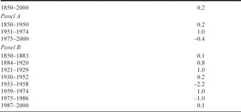
Since we found it impossible to distinguish the part that corresponded to capital incorporated into the improved land, we settled for a crude estimate of the land stock. The first step was to elaborate yearly figures for the stock of land. Unfortunately, estimates for total agricultural land only exist at some benchmarks before the late 1950s that we have interpolated to derive annual figures and, then, adjusted for the economic cycle with the deviations from the Hodrick-Prescott trend in agricultural output.Footnote 30 Next, we converted hectares of land into a stock by weighting each type of land by its price at two different benchmark years (1931 and 1985) and splicing the resulting quantity indices into a single Laspeyres index for the entire period considered.Footnote 31 Since the land stock grew little over the long run (Table 2), and certainly much less than capital and labor, its inclusion in the growth accounting exercise pushes TFP growth upwards.Footnote 32
Labor Input
The appropriate measure of labor input is the flow of services for production emanating from this factor.Footnote 33 Hence, our task is to estimate
CHANGE IN THE LAND STOCK, 1850-2000 (annual average logarithmic rates in percent)

Sources:
See the text and note to Table 1.
the labor force cross-classified by as many attributes as possible to capture its heterogeneity. Although census and survey data from 1850 to 1954 do not make it possible to match a worker's individual income with his or her age or education, we have been able to classify the population by gender, two different age attributes (adult, child), branchof activity, income, and hours worked.Footnote 34 The first step in the construction of labor input series was to put together yearly employment figures for the four main sectors of the economy (agriculture, forestry, fishing, industry construction, and services) on the basis of population censuses.Footnote 35 Employment in these four large sectors was then distributed into their branches. Up to 1955 population censuses allowed us to cross classify working population into 19 industries up to 1900, 21 industries for 1900-1910, 22 for 1911-1950, and 24 thereafter.Footnote 36 Lack of data for 1850-1900 forced us to breakdown manufacturing employment into its branches by assuming that its distribution in 1900 was representative of the entire period.Footnote 37
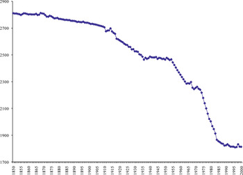
The second step was to convert the data on the number of workers into days and then hours worked per year for the period 1850-1954. We assumed that each full-time worker was employed 270 days per annum in industry and services. Such a figure results from deducting Sundays and religious holidays plus an allowance for illness.Footnote 38 This assumption is consistent with contemporary testimonies and supported by the available evidence.Footnote 39 In agriculture, however, contemporary and historians' estimates point to a lower figure for the working days per occupied.Footnote 40 Throughout most of the nineteenth and early twentieth century, peasants were only fully employed during the summer; they were idle for up to four months every year and worked outside agriculture. Therefore, we assumed that each male worker devoted 240 of his 270 days to farming and the 30 remaining days to services. The resulting figures for hours per worker/year declined over time (Figure 3) and varied greatly.Footnote 41
HOURS PER WORKER-YEAR, 1850-2000 (semilog scale)

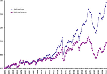
The amount of labor, measured by total hours worked, presents a moderate increase over the long run (Figure 4).Footnote 42 Labor force grew moderately up to World War I while it accelerated during the 1920s and early 1930s, partly as a result of population growth and rural-urban migration. Labor quantity rose again during the Golden Age (1951-1974). The “transition to democracy” decade (1975-1986) witnessed a dramatic employment destruction driven by the oil shocks and the exposition of traditionally sheltered industrial sectors to international
LABOR INPUT AND QUANTITY, 1850-2000 (1850=100) (semilog scale)

competition. Labor market deregulation, a marked increase in female participation rate, and the arrival of immigrants—only in the last decade of the twentieth century—are beneath the rise in employment since 1987. Population growth and the decline in hours per worker explain, in a proportion of two to one, most of the moderate increase in the labor quantity over the long run. Hours per worker and per year shrank from 2,800 at mid-nineteenth century to 1,800 by the end of the twentieth century (Figure 3).Footnote 43
Throughout the hundred and fifty years of modern economic growth considered here, the rise of the quantity of labor measure in the total amount of hours worked was mainly determined by population growth. However, a closer look reveals how other factors at work conditioned its evolution across different long swings. For example, the declining hours per worker/year over 1914-1936, a result of the gradual adoption of the eight hours per day standard associated to increasing urbanization and structural change. In the 1920s falling hours per worker went hand-in-hand with a significant increase in the employment rate, also linked to structural transformation. Between the early 1930s and 1950s the rising share of the working-age population, a result of the demographic transition, made up for the contraction in participation and employment rates. In the Golden Age, the growth in total hours worked was slowed by a significant fall in annual hours worked per employed person and a rise in the dependency rate (the ratio of nonworking to working-age population). Later, during the “transition to democracy” (1975-1986), a dramatic contraction in the quantity of labor took place as a result of the surge in unemployment, a fall in the participation rate, and a decline in yearly hours per worker. Since Spain's entry in the European Union (1986), the brisk recovery in the participation and employment rates help explain the increase in the total hours worked.
The third phase in the construction of the labor input is to weight each category of workers by its average nominal earnings.Footnote 44 The quality and availability of wage data necessary to construct these estimates vary enormously through time.Footnote 45
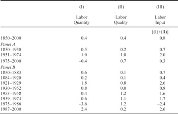
Figure 4 reports the evolution of labor input and labor quantity (unweighted hours worked) from 1850 to 2000. Although the evolution of labor input generally parallels that of labor quantity, the labor input does grow more rapidly because of shifts in labor composition (“quality”), which capture improvements in workers' skills and, hence, human capital.Footnote 46 Three phases stand out in the evolution of the labor input: the 1920s, the Golden Age, and 1986-2000 (Table 3). Labor quality improvements contributed significantly to labor input growth in the interwar and the Golden Age and compensated for a decline in labor quantity during the “transition to democracy” (1975-1986). But it added little following Spain's accession to the European Union in 1986.Footnote 47
LABOR QUANTITY, QUALITY, AND INPUT GROWTH, 1850-2000 (annual average logarithmic rates in percent)

Note:
Labor Quantity is the unweighted hours worked; Labor Quality, improvements in labor's skills (human capital); Labor Input, which adds up labor quantity and quality, is the flow of services emanating from labor.
Sources:
See the text and Prados de la Escosura and Rosés, “Proximate Sources,” and the note to Table 1.
Factor Shares
In addition to the real factor inputs described above, we need to know the elasticity of output with respect to each input (θi) in order to compute the sources of growth. Under the restrictive assumption of perfect competition and constant returns to scale, these elasticities can be proxied by the share of each factor's returns in national income. Such an assumption might be objectionable as restrictions on competition and monopolistic practices are common in Spanish history.Footnote 48 If monopolists earned rents, our “naive” results (obtained under the assumption of perfect competition) would bias total factor productivity growth.Footnote 49 Yet, even if this were the case, our results (as we shall see) would not be significantly altered.
Up to 1954 labor returns were directly estimated. From 1954 onwards we derived factor shares from the official national accounts that we previously spliced together.Footnote 50 To measure labor income correctly, it is crucial to establish what proportion of the income of proprietors, unpaid family workers, self-employed, and retired workers represent returns to labor.Footnote 51 We have assumed that entrepreneurs and self-employed workers have a labor income equal to the average compensation of employees in their corresponding industry.Footnote 52 Dividing total labor (including self-employed) compensation by GDP, we obtained the share of labor. The lack of information on land rents forced us to derive the land share as the residual after deducting labor outlays from agricultural gross value added. This method implies no returns to capital from agriculture and, hence, tends to overstate the share of land in GDP.Footnote 53 The share of capital was then obtained as a residual after deducting labor and land returns from GDP at factor costs.Footnote 54
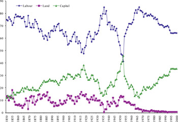
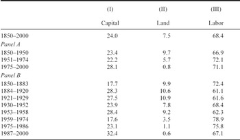
Figure 5 shows the evolution of the shares of land, capital, and labor in GDP. On average, for the one-and-a-half centuries considered, our factor shares are 0.08 for land, 0.24 for capital—that is, 0.32 for property—and 0.68 for labor, that roughly match the 1/3 and 2/3 weights conventionally employed in growth literature. Average shares vary, with labor fluctuating around two-thirds, except in the phase of accelerating growth, 1959-1974, and during the critical years of the “transition to democracy,” 1975-1986 (Table 4). Interestingly, the peak of labor share corresponds to years in which skilled workers represented a larger proportion of the labor force and income inequality was lower.Footnote 55
FACTOR SHARES IN GDP, 1850-2000 (percent)

The relative instability of the factors shares contrasts with the conventional assumption of stability. This is largely a consequence of data limitations, but the share fluctuations can be explained. Between mid-nineteenth century and World War I, the growing importance of capital can be attributed to rising investment rates and technological change favoring capital. The rise in inequality (from the late 1890s to the end of World War I) coincided with a return to strict protectionism, which favored land owners.Footnote 56 In the interwar years, the labor share grew significantly. Institutional labor market reforms favoring workers, especially the reduction in the number of working hours per day and the increasing voice of trade unions, contributed to a rise in wages relative to property incomes. Also the increase in the human capital endowment of the workforce influenced the expansion of labor. The early years of Franco's regime witnessed a sharp decrease in the labor share, an

outcome of dictatorship's economic policy that implied a redistribution of income towards property owners. Since the mid-1950s a rapid increase in labor share took place that peaked by the late 1960s, when pre-Civil War levels were recovered. The elevated labor shares reflected human capital accumulation and the more liberal economic policies that accompanied growth and structural change in the late Francoist regime. Since the early 1970s, however, the capital share in GDP has tended to grow at expenses of labor.
MAIN TRENDS IN TOTAL FACTOR PRODUCTIVITY
The sources of long-run growth in Spain are displayed in Table 5.Footnote 57 Over the one-and-a-half century considered, TFP and broad capital (physical and, to less extent, human capital) appear to be equally responsible for GDP growth. The early 1950s represent a divide between a hundred years of moderate growth dominated by factor accumulation, and half a century of fast growth led by total factor productivity, with 70 percent of the more rapid GDP growth after 1950 coming from efficiency gains.
SOURCES OF GDP GROWTH, 1850-2000 (annual average logarithmic rates in percent)

Sources:
See Tables 1-4 and the text and note to Table 1.
A closer look at long swing intervals reveals that prior to 1950, total factor productivity played a far from negligible role in 1850-1883 and the 1920s (Table 5). As a source of growth, TFP may actually be underestimated as it does not include the additional capital accumulation that results from a productivity increase.Footnote 58
Total factor productivity led GDP growth during 1953-1986, a period that included both the Golden Age and the decade of sluggish growth during the transition from dictatorship to democracy. TFP contributed to more than half of GDP growth during the Golden Age, and two-thirds to its acceleration over the previous hundred years, a large role by historical standards. In fact, about two-thirds and four-fifths of the acceleration in GDP growth in 1953-1958 and 1959-1974 over the previous long swings (1930-1952 and 1953-1958, respectively) were due to TFP, and in 1975-1986 efficiency gains prevented a GDP contraction. Since Spain has joined the European Union (1986), employment creation and the recovery of physical capital accumulation has offset the slowdown in total factor productivity.
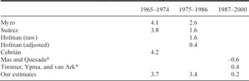
How do our results compare with those of empirical economists for the post-1964 era? A glance at Table 6 suggests that our growth rates
TFP GROWTH, 1965-2000: ALTERNATIVE ESTIMATES (annual average logarithmic rates in percent)

* Excluding residential structures from capital input.
Sources:
Suárez, “Economías de escala”; Hofman, “Economic Development”: 256, 1973-1989; Myro, “Evolución de la productividad”: 1966-1974, 1975-1981; Cebrián, “Fuentes del crecimiento”: 1964-1973; Timmer and Van Ark, “Information and Communications Technology”; Mas and Quesada, Nuevas tecnologías: 283, 1985-2002; for our estimates, see Table 5 and the text.
are in line with those available for 1965-1974 and for 1987-2000. And they too suggest that TFP growth slowed after Spain's admission into the European Union.
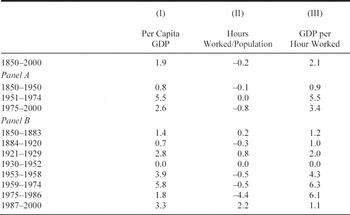
Modern economic growth is associated with improvements in GDP per head but, so far, the discussion has been focused on absolute GDP trends. We need, therefore, to establish the connection between increases in per capita GDP and efficiency gains. Table 7 provides an intermediate stage, namely, the decomposition of output per head into hours per person and output per hour. Although hours worked per person declined in the long run trend, the 1920s and the post-1986 years show a marked increase in the labor quantity per head. Labor productivity, in turn, grew at a modest pace before 1920 and since 1987, and stagnated in the 1930s and 1940s. But it experienced impressive gains between 1953 and 1986. Sluggish labor productivity lies beneath weak improvements in GDP per head, with the exception of the last quarter of the twentieth century when labor quantity and productivity evolve inversely. Hours worked dropped during the “transition to democracy,” but the decline was more than offset by the productivity surge associated to industrial restructuring and shifts of resources away from agriculture and traditional industrial sectors. Since 1987 the productivity slowdown has been compensated by a strong increase in hours worked. As Riccardo Faini put it for the Euro zone, Spain seems to have been unable to combine employment and productivity growth since the mid-1970s.Footnote 59
PER CAPITA GDP GROWTH AND ITS COMPONENTS, 1850-2000 (annual average logarithmic rates in percent)

Sources:
See the text, Prados de la Escosura and Rosés, “Proximate Sources,” and the note to Table 1.
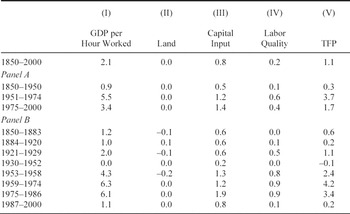
Labor productivity trends are determined, in turn, by human and physical capital/labor ratios and efficiency gains. Table 8 provides the decomposition of labor productivity growth. The main result is that TFP accounts for half the increase in labor productivity over the one-and-a-half centuries considered. Furthermore, the fluctuations in labor productivity growth parallel changes in TFP.
Conclusion
The main arguments of the article can now be restated. First of all, factor accumulation, especially capital, and TFP growth seem to have been complementary for GDP and labor productivity growth over the long-run Spanish experience suggests a two-stage process in which improving efficiency appears as a complex learning process that takes place once growth has been initiated by allocating additional capital and labor to production.Footnote 60 Abstention, rather than ingenuity, dominated

long-run growth in Spain up to 1950. Thereafter, TFP growth, a “free lunch” to use Joel Mokyr's words, drove economic progress. Our results therefore run counter to P. Krugman's intuition that growth on the basis of capital accumulation ultimately slows.Footnote 61
Second, we accept that our growth accounting yields only a range of best estimates and that our coverage of factor accumulation is far from perfect. However, it is important not to exaggerate the skepticism. Alternative measures of factor accumulation and factor shares lead to similar results for TFP growth.
Third, our results do not appear unusual in international perspective, where there is growing evidence suggesting that factor accumulation prevailed over efficiency gains in the early stages of development. Factor accumulation seems to play a role during the transitional phase to long-run growth.Footnote 62 Once modern economic growth is under way, TFP tends to perform a more significant part. Indeed, TFP provided at least one-quarter of British GDP growth between 1780 and 1860, a proportion that increases to three-eighths when embodied technological change is taken into account.Footnote 63 Slow TFP growth has also been confirmed for the nineteenth century in the United States.Footnote 64 Long-run assessments for countries in the European Periphery such as Portugal and Turkey show similar results.Footnote 65 During the last four decades of the twentieth century, developing countries exhibited growth rates dominated by factor accumulation.Footnote 66 In modern Spain, as in Britain during the Industrial Revolution, TFP accounted for most of labor productivity acceleration.Footnote 67 Does the ability to absorb and to adapt productively foreign ideas and technology depend on a country's development level?Footnote 68 Comparative historical research will be needed before this hypothesis can be put to the test.