Economic histories of the United States identify a period of rapid economic growth beginning in the 1820s and lasting to the outbreak of the Civil War (e.g., David Reference David1967; Davis Reference Davis2004), during which per capita income, real wages, and most other economic indicators of the standard of living increased considerably (e.g., Costa and Steckel Reference Costa, Steckel, Richard and Floud1997; Goldin and Margo Reference Goldin, Margo, Goldin and Rockoff1992; Margo Reference Margo2000). Despite this progress, the United States entered the Civil War having taken a step backward in another important facet of the standard of living—health. The best known manifestation of this pattern was the decline in average stature observed in the native-born Northern white male birth cohorts of the 1830s and 1840s (A’Hearn Reference A’Hearn, Komlos and Baten1998; Floud et al. Reference Floud, Fogel, Harris and Hong2011; Fogel Reference Fogel, Engerman and Gallman1986; Komlos Reference Komlos1987; Margo and Steckel Reference Margo and Steckel1983; Zimran Reference Zimran2019).Footnote 1 Known as the Antebellum Puzzle because rising incomes would typically be expected to improve health (Fogel Reference Fogel1994; McKeown Reference McKeown1976), this discrepancy between trends in economic and biological indicators of living standards has complicated the interpretation of the welfare effects of early modern economic growth in the United States. Despite the importance of this pattern to U.S. economic history, questions remain regarding its causes.
The economic growth of the antebellum period was caused, in part, by a contemporaneous Transportation Revolution that transformed the American continent and economy by expanding transportation infrastructure into large areas that were previously unlinked and undeveloped (Taylor Reference Taylor1951). Although economic theory shows that the impact of transportation on health may be positive or negative, it has long been suspected that the antebellum transportation expansion may have contributed to the contemporaneous decline in health (Cuff Reference Cuff2005; Haines, Craig, and Weiss Reference Haines, Craig and Weiss2003; McGuire and Coelho Reference McGuire and Coelho2011; Yoo Reference Yoo2012). But the effect of transportation on health in the antebellum United States remains empirically unclear because of data limitations (described by Atack Reference Atack2013) and methodological constraints faced by prior research.
In this paper, I exploit recent data and methodological advances to determine the effect of transportation improvements on average stature in the rural United States in the period 1820–1847. This period encompasses the decline in average stature that constitutes the Antebellum Puzzle (Craig Reference Craig, Komlos and Kelly2016; Zehetmayer Reference Zehetmayer2011). It also captures infrastructure expansion on a massive scale into previously isolated areas, consisting largely of construction of the canal network in the Northeast and Midwest and of expansions in navigability of the Mississippi River system and its major and minor tributaries through improvements in steamboat technology and the clearance of hazards to navigation. I focus on the rural population because this is the sector in which transportation is hypothesized to have contributed to declining health and because this was the sector in which the bulk of the decline in stature occurred (Steckel Reference Steckel1995).Footnote 2
My analysis is based on two main data sources that together enable me to link individuals’ adult height—a common measure of health in historical settings that reflects net nutritional status in childhood and adolescence (Floud et al. Reference Floud, Fogel, Harris and Hong2011; Steckel Reference Steckel1995)—to the transportation linkage status of their county-year of birth.Footnote 3 In particular, I use height data from the records of enlisters in the Union Army (Records of the Adjutant General’s Office 1861–1865). This source provides information on the heights, counties of birth, and birth cohorts of 25,566 native-born rural white men in the birth cohorts of 1820–1847 in the Northeast and Midwest regions of the United States. To describe the development of the transportation network in the antebellum United States, I use Geographic Information Systems (GIS) shape files created by Atack (Reference Atack2015, Reference Atack2016, Reference Atack2017), which provide the location and opening date of all canals, railroads, and steamboat-navigable waterways in the antebellum United States. This source marks an improvement over the transportation data available in previous investigations of the link between transport and health in the antebellum United States (Haines, Craig, and Weiss Reference Haines, Craig and Weiss2003; Yoo Reference Yoo2012), for which only approximations of the state of the transportation network in a single year were possible (Atack Reference Atack2013). I use these data to compute Donaldson and Hornbeck’s (Reference Donaldson and Hornbeck2016) market access statistic for all counties east of the Mississippi River for each year 1820–1847, which is my main measure of transportation linkage.
The main empirical challenge of this paper is to determine the impact of transportation improvements on height while addressing the possibility that any correlation between the two might be driven by omitted and potentially unobservable variables. For instance, local characteristics might have spurred economic growth, attracting transportation, affecting health, and creating a spurious relationship between the two. Two aspects of my analysis, made possible by the new data and methods that I use to measure transportation linkage, enable me to address these concerns to an extent not possible in prior studies of the link between transportation and health in the antebellum United States (Cuff Reference Cuff2005; Haines, Craig, and Weiss Reference Haines, Craig and Weiss2003; Yoo Reference Yoo2012). First, the panel structure of the data on a county’s transport linkage enables me to estimate specifications that include county fixed effects, capturing location-specific characteristics that might create a spurious relationship between transportation and height. Second, my use of the market access statistic to measure transportation linkage makes it possible to control directly for potentially endogenous transportation linkage and to identify the effects of market access on health using variation generated by construction elsewhere in the network, which is less likely to be related to confounding factors that might relate construction in a county to its health (Donaldson and Hornbeck Reference Donaldson and Hornbeck2016; Hornbeck and Rotemberg Reference Hornbeck and Rotemberg2019).
I find a negative effect of transportation linkage, as measured by market access in the county-year of birth, on health, as measured by adult stature. The magnitude of this relationship is large: In my preferred specification, I find that a one-standard-deviation increase in market access reduced average stature by 0.14 inches. To put this figure in perspective, average stature in my data declined by 0.82 inches from 1820 to 1847.Footnote 4
I also investigate one possible mechanism for the negative effect of transportation on average stature, which attributes the deleterious impact of transportation to the increases in population density that transportation generates. I refer to this as the local development mechanism. In combination with insufficient sanitation and public health infrastructure in this period, such concentration of population would have made previously undeveloped locations less healthy (Costa Reference Costa1993; Floud et al. Reference Floud, Fogel, Harris and Hong2011; Steckel Reference Steckel1995). Consistent with this mechanism, I find a positive impact of market access on population density. Heterogeneity in the impact of market access on population density and stature provides further support for this mechanism. In particular, I find that the effects of market access on increasing population density were stronger in counties where the suitability for wheat and corn production was greater (Food and Agriculture Organization 2002). This result is consistent with the importance of these goods in long-distance trade (Atack and Passell Reference Atack and Passell1994, pp. 292–94): Counties that were better able to produce these grains would have benefited more from improved linkage to markets, leading to greater population growth in these counties.Footnote 5 I also find that the negative impact of market access on stature was stronger in counties with greater wheat and corn suitability. Thus, counties where population density increased the most in response to rising market access were those where the deleterious effect of market access on average stature was the greatest. This is consistent with rising population density contributing to the decline in stature.
This paper contributes to the literature seeking to understand the causes of the deterioration of average stature in the antebellum United States (e.g., Costa Reference Costa1993; Haines, Craig, and Weiss Reference Haines, Craig and Weiss2003; Komlos Reference Komlos1998; Steckel Reference Steckel1995). Several theories have been proposed to explain this decline (Floud et al. Reference Floud, Fogel, Harris and Hong2011), and much evidence consistent with these theories has been marshaled. But well-identified causal evidence that any particular factor caused declines in height in the antebellum United States is lacking. In this paper, I provide direct and plausibly causal evidence as to a potential explanation for this puzzle by showing that the effect of market access on average stature, combined with the rise in market access over the antebellum period, can explain 37 percent of the decline in stature.Footnote 6 Moreover, by providing evidence consistent with the local development mechanism, which attributes the decline in health to epidemiological factors, the paper contributes to the debate over whether the changing epidemiological environment was a contributor to the antebellum decline in health (e.g., Costa Reference Costa1993; Komlos Reference Komlos2012).
This paper also brings the impacts of the antebellum period’s transportation improvements into sharper focus, adding to the literature on the impacts of transportation improvements in the nineteenth-century United States. Recent data improvements have enabled scholars to better determine the causal effects of transportation improvements in this context, but the focus has typically been on the impact of railroads on economic development (e.g., Atack et al. Reference Atack, Bateman, Haines and Margo2010; Donaldson and Hornbeck Reference Donaldson and Hornbeck2016; Hornbeck and Rotemberg Reference Hornbeck and Rotemberg2019). This paper broadens the scope of analysis of such work to health impacts and adds to the literature studying the effects of canal construction and expansions in river navigability,Footnote 7 which were the main transportation improvements in the period that I study.
This paper also makes a contribution outside of the nineteenth-century United States. Although there is a large literature describing the impacts of transportation improvements on a variety of economic outcomes,Footnote 8 such as urbanization and industrialization, the effects on health have received far less empirical attention and are not understood as well. To my knowledge, only a few studies (Ahmad Reference Ahmad2019; Burgess and Donaldson Reference Burgess and Donaldson2012; Tang Reference Tang2017) exist determining the causal effect of transportation on health in specific cases.Footnote 9 This paper contributes to this literature by providing an analysis of the effect of transportation on health in the context of a large and historically important infrastructure expansion. It shows, with attention to causality, that despite the well-known economic benefits of this expansion, it had a negative impact on health.
TRANSPORTATION AND HEALTH IN THE ANTEBELLUM UNITED STATES
The Antebellum Puzzle
Modern economic growth in the United States began around 1820 (David Reference David1967). This was the beginning of a long process that eventually brought the United States to world economic leadership and led to a drastic long-run improvement in living standards, including health (Fogel Reference Fogel1994). In the shorter run, however, the welfare effects of modern economic growth are less clear. Whereas income per capita and wages rose in the first few decades of U.S. modern economic growth (Costa and Steckel Reference Costa, Steckel, Richard and Floud1997; Goldin and Margo Reference Goldin, Margo, Goldin and Rockoff1992; Margo Reference Margo2000), health declined. The average height of native-born Northern white males in the United States declined by between 0.65 and 1.25 inches (depending on the estimate) between the birth cohorts of 1830 and 1860 (A’Hearn Reference A’Hearn, Komlos and Baten1998; Floud et al. Reference Floud, Fogel, Harris and Hong2011; Komlos Reference Komlos1987; Zimran Reference Zimran2019). It was not until nearly the birth cohort of 1900 that average stature would begin to rise again (Fogel Reference Fogel, Engerman and Gallman1986; Steckel Reference Steckel1995; Zehetmayer Reference Zehetmayer2011).Footnote 10 Moreover, between the first and second quarters of the nineteenth century, life expectancy at age 10 for males declined by about 3 years (Fogel Reference Fogel, Engerman and Gallman1986).
Despite a large body of research devoted to describing and debating the decline in health in the antebellum United States, a definitive explanation for it has not been identified. Recent scholarship favors a combination of two mechanisms (Floud et al. Reference Floud, Fogel, Harris and Hong2011).Footnote 11 The first, the disease explanation, holds that a variety of forces led to an increased exposure to disease during the antebellum period (Costa Reference Costa1993; Fogel Reference Fogel, Engerman and Gallman1986; Steckel Reference Steckel1995). The second, the food price explanation, argues that the decline in height was the result of a rise in the relative price of food that led individuals to substitute away from food consumption toward the consumption of manufactures (Komlos Reference Komlos1987; Komlos and Coclanis Reference Komlos and Coclanis1997). Distinguishing between these explanations is important in determining the welfare effects of early modern economic growth. Under the disease explanation, the decline in health was the product of a negative externality of economic growth, the welfare effects of which were, thus, ambiguous; but, under the food price explanation, it was the product of utility-maximizing choice, implying that welfare improved unambiguously during this period.
Although these explanations hypothesize that forces beyond the expansion of transportation infrastructure in the period played a role in spreading disease and changing relative prices, both also posit a role for transportation. Under the disease explanation, transportation may have carried disease along with freight and passengers, bringing infection to places that it had once been unable to reach (e.g., Tang Reference Tang2017). Indeed, disease was prevalent in urban areas in the antebellum United States (Floud et al. Reference Floud, Fogel, Harris and Hong2011), and transportation linkages in rural areas may have facilitated the spread of disease from urban areas to previously salubrious rural ones. Transportation may also have generated increases in local development (e.g., Atack et al. Reference Atack, Bateman, Haines and Margo2010; Donaldson and Hornbeck Reference Donaldson and Hornbeck2016). These gains may have reduced health as greater population density or urbanization increased exposure to disease by increasing contact between individuals and through the sanitation consequences of greater concentrations of population (Costa Reference Costa1993; Steckel Reference Steckel1995). Under the food price explanation, transportation may have affected health through its impact on relative prices. The originally rural areas being linked to the transportation network in this period were largely food producing. Transportation linkage in this setting would tend to increase the farm-gate price of food relative to that of manufactures. Under certain price and income elasticities, this would induce individuals to consume less food (or reduce expenditure on food), reducing health (Komlos Reference Komlos1987; Komlos and Coclanis Reference Komlos and Coclanis1997).
Importantly, transportation need not have had a negative effect on health at all. Indeed, the rising incomes generated by new transport links (e.g., Donaldson and Hornbeck Reference Donaldson and Hornbeck2016) might have contributed to improving health, just as the rising incomes of the period were expected to improve health. Indeed, Baten and Fertig (Reference Baten and Fertig2009) find evidence of such a positive effect in Germany in the late nineteenth century.
The empirical evidence underlying both of these explanations is limited. Largely as a result of limited data availability for the antebellum period, much of the evidence that has been marshaled in support of these explanations is suggestive, based either on cross-sectional correlations or on national time series. To my knowledge, there does not exist strong causal evidence showing that any particular force caused declines in height.Footnote 12
Among this prior research is the study of Haines, Craig, and Weiss (Reference Haines, Craig and Weiss2003), to which the present paper is most closely related. Haines, Craig, and Weiss (Reference Haines, Craig and Weiss2003) study the relationship between height (also using data from the Union Army records) and mortality, on the one hand, and transportation and a variety of measures of local agricultural production on the other. They find that transportation presence was associated with average stature being lower by about 0.25–0.30 inches. The data and methods available at the time that their study was carried out prevent the results from being given a strong causal interpretation. First, Haines, Craig, and Weiss’s (Reference Haines, Craig and Weiss2003, pp. 391–92) measure of transportation linkage was an indicator of whether a county was on a navigable waterway in 1840—the most detailed data available at the time. Besides the obvious limitations coming from the lack of time variation in these data, Atack (Reference Atack2013, p. 318) describes the difficulty in ascertaining the precise location of these waterways. Donaldson and Hornbeck (Reference Donaldson and Hornbeck2016) also point out the limitations of a binary indicator of transportation linkage, which does not capture the impacts of construction elsewhere in the network. Moreover, Haines, Craig, and Weiss (Reference Haines, Craig and Weiss2003) were not able to effectively address issues of endogeneity in the relationship between transport and health. A host of factors may have affected both transport linkage and health, creating a spurious relationship between the two. Thus, while Haines, Craig, and Weiss’s (Reference Haines, Craig and Weiss2003) results are consistent with transportation contributing to the antebellum decline in health, convincing causal evidence does not yet exist. Similar concerns constrain the related results of Cuff (Reference Cuff2005) and Yoo (Reference Yoo2012). Moreover, no prior evidence exists regarding the mechanism by which transportation may have affected health in this context. This paper is able to advance on all of these fronts, providing a clearer view of the role of the Transportation Revolution in shaping the evolution of health in the antebellum United States.
Transportation in the Antebellum United States
The first major internal improvement in the United States was the Erie Canal, completed in 1825. Though coastal shipping was well developed by this point and some turnpikes had emerged, the interior of the continent was virtually isolated from the Atlantic Coast. Thus, the Erie Canal was revolutionary, dramatically easing interregional trade between the Northeast and the (upper) Midwest. The financial success of the Erie Canal sparked a surge in canal construction in the Northeast and Midwest, with the greatest investment in canal construction occurring in the decade ending 1845. Although many of these canals were financially unsuccessful, they had important impacts on the economic development of the areas through which they passed and on the counties that they linked to the broader market, increasing land values and reducing transport costs. The new canals also reshaped trade patterns, with long-distance trade being rerouted from the Mississippi and Ohio rivers to the Great Lakes and Erie Canal. Another main transportation innovation of the antebellum period was the steamboat, with improvements in steamboat construction technology and the clearance of hazards to navigation gradually opening first the main rivers and then the smaller tributary rivers to steam navigation. The first railroads were also built in the antebellum period, but largely in the 1850s—after the study period of this paper (Atack and Passell Reference Atack and Passell1994, pp. 150–59).
The impact of improved water transportation on agriculture is well documented. Canals and steamboats made shipments of meat and grain from the Midwest to the markets of the Northeast and Europe possible for the first time. Indeed, shipments from western states “grew at an average annual rate of over 10 percent from the 1830s as production was increasingly oriented toward more distant markets” (Atack and Passell Reference Atack and Passell1994, p. 162). Competition from Midwestern farms also caused a shift in the production of Northeastern farms toward more locally oriented goods, such as dairy (Atack and Passell Reference Atack and Passell1994, pp. 160–71).
The impacts of canal construction and improvements in river navigability on nonagricultural outcomes, such as industrialization, have received less attention. However, some of the recent research on the impacts of railroads in the antebellum United States suggests that expanded water transportation may also have had an effect on other forms of development. For instance, Hornbeck and Rotemberg (Reference Hornbeck and Rotemberg2019) find that the railroad increased manufacturing, using data from the 1860 Census of Manufactures. Such a potential impact of transportation is particularly important in the case of the Northeast, where farming became less important after expanding water transportation increased Midwestern competition, as discussed above. Atack et al. (Reference Atack, Bateman, Haines and Margo2010) also find that the railroad caused an increase in urbanization in the Midwest during the 1850s. All of these impacts of transportation provide potential channels for transportation to have affected health. Among many other possible outcomes, the income gains coming from greater ability to produce agricultural and industrial products for larger markets may have generated population growth, both due to Malthusian responses (Ahmad Reference Ahmad2019) and due to in-migration. This greater population concentration, in turn, may have led to a greater prevalence of disease.
DATA AND EMPIRICAL APPROACH
Height Data
The main outcome on which I focus is adult height. This measure, which is commonly used as an indicator of health in historical and developing contexts (e.g., Deaton Reference Deaton2007; Floud et al. Reference Floud, Fogel, Harris and Hong2011), is unique in the antebellum United States in that it is perhaps the only measure that can provide insights into health for the bulk of the population for a number of years.Footnote 13 Average stature is increased by greater calorie and protein consumption and by a better sanitary environment, while strenuous physical labor, malnutrition, and chronic disease tend to decrease it (Deaton Reference Deaton2007; Floud et al. Reference Floud, Fogel, Harris and Hong2011; Steckel Reference Steckel1995).Footnote 14
Data on the heights of men born in the United States in the years 1820–1847 are available from the records of enlistments in the Union Army during the Civil War (Records of the Adjutant General’s Office 1861–1865). This widely used source is informative of height, place of birth, age, year of enlistment, and place of enlistment. I combine three random samples of this source. The first comes from the Union Army Project (Fogel et al. Reference Fogel, Costa, Haines, Lee, Nguyen, Pope, Rosenberg, Scrimshaw, Trussell, Wilson, Wimmer, Kim, Bassett, Burton and Yetter2000), which provides information on a random sample of approximately 40,000 individual observations from the original records. The second is provided by Cuff (Reference Cuff2005), yielding approximately 12,000 additional observations of men born in the state of Pennsylvania and serving in Pennsylvania regiments. Finally, I collected and digitized approximately 3,000 additional observations from the original records.
As is standard in the use of these data, I restrict the sample to white men born in the Northeast or the Midwest. Coverage of the South is sparse because of the very limited representation of southerners in the Union Army. I also exclude individuals measured before age 18, which implies that the youngest birth cohort included in the sample is that of 1847. I also exclude birth cohorts older than 1820 because of the relative lack of representation of these older cohorts in the military. Finally, I limit the sample to those for whom county of birth, height, birth year, and age of measurement are known.Footnote 15 After imposing these restrictions, 31,402 observations remained. For a subset of these observations, the county of enlistment could also be determined.
I restrict attention to individuals born in counties that had no urban population in 1820, reducing the sample to 25,566 individuals.Footnote 16 I make this restriction for three main reasons. First, Steckel (Reference Steckel1995, p. 1927) points out that understanding patterns in height in the antebellum United States requires a focus on the rural sector. This sector encompasses the bulk of the population and drove the bulk of the decline in stature. Moreover, the decline in stature of the urban sector is less puzzling than the decline of the rural sector, as the growing cities of the period were noted as unhealthy (e.g., Floud et al. Reference Floud, Fogel, Harris and Hong2011; Haines Reference Haines2004); the challenge is to explain the health declines of rural areas. Second, transport linkages are not hypothesized as explanatory factors for declining stature in urban areas—if anything, better transport linkages between cities and food-producing areas would tend to improve health (Zehetmayer Reference Zehetmayer2013). It is the effect of transport on rural areas that is important in searching for an explanation for the Antebellum Puzzle. Finally, many transport links were built to link the interior to specific urban areas (e.g., the Erie Canal, Pennsylvania’s Main Line, the C&O Canal), implying that endogeneity of transport is particularly severe for these areas.
A key question regarding the enlistment data is whether they are representative of the broader population of interest—native-born rural white males in the Northeast and Midwest in the birth cohorts of 1820–1847. The oversampling of Pennsylvanians is one obvious concern, which I address by reweighting so that the distribution of states of residence matches that of the 1860 census. Another concern is that entrance into the Union Army was subject to a minimum height requirement. Although this requirement was not stringently enforced, the left tail of the height distribution was underrepresented.Footnote 17 The common approach in the historical heights literature is to use a reduced-sample maximum likelihood estimator that omits any observations below the cutoff point and assumes normality of the stature distribution (A’Hearn Reference A’Hearn, Komlos and Baten1998). In the present context, however, there were a number of individuals who were able to enlist despite the restriction, suggesting that this is not a completely proper modeling of the role of the minimum height requirement in enlistment. As a result, the findings reported below do not use such a truncation-corrected regression. Online Appendix C repeats the main results with this method of analysis, showing that the results are robust to it.
A more nuanced concern is that selection into military service was nonrandom (Bodenhorn, Guinnane, and Mroz Reference Bodenhorn, Guinnane and Mroz2017). This concern is mitigated by the fact that nearly half of the population at risk for military service enlisted (Zimran Reference Zimran2019). For this reason, the Union Army data are considered to be representative of the white male population of the Northern states (Fogel et al. Reference Fogel, Costa, Haines, Lee, Nguyen, Pope, Rosenberg, Scrimshaw, Trussell, Wilson, Wimmer, Kim, Bassett, Burton and Yetter2000). This view is reinforced by Zimran’s (Reference Zimran2019) formal investigation of bias in historical height data sources, which finds that the height data in the Union Army records suffer from little bias.Footnote 18 Moreover, my inclusion of county, birth year, and enlistment year fixed effects in all main specifications addresses many of the possible forms of this bias, such as changing incentives for enlistment over time (Bodenhorn, Guinnane, and Mroz Reference Bodenhorn, Guinnane and Mroz2017) and differences over counties in ideology (Zimran Reference Zimran2019, Reference Zimran2020a). But, in the end, I am not able to rule out the possibility that selection may have varied by county-birth cohort such that selection changed in response to transportation, creating a relationship between observed height and transportation that does not reflect the relationship between actual height and transportation.Footnote 19 Despite this limitation, the Union Army data provide the best available view of trends in health during the antebellum period.
Transportation Data
Information on transportation infrastructure is given by GIS shape files created by Atack (Reference Atack2015, Reference Atack2016, Reference Atack2017). These files provide the location of all steamboat-navigable rivers, canals, and railroads in the continental United States constructed or opened prior to 1914.Footnote 20 These files do not provide information on the location of turnpikes, but this omission is unlikely to have a major effect on results because of the high costs of wagon transportation (Donaldson and Hornbeck Reference Donaldson and Hornbeck2016; Taylor Reference Taylor1951). These shape files also provide the year in which any particular segment of canal, rail, or river first became available (and, if applicable, when it ceased to be).
I use these data to create two measures of transportation linkage. The first is a simple measure that takes a value of one in years in which a county was linked to water or rail transportation, and zero otherwise.Footnote 21 While it is a straightforward measure and is used in prior research (e.g., Atack et al. Reference Atack, Bateman, Haines and Margo2010; Haines, Craig, and Weiss Reference Haines, Craig and Weiss2003), this faces some important limitations. First, it does not capture the impacts of new forms of transportation entering already linked areas. Relatedly, it treats all transportation links as equivalent, though it is clear that they would not be. More importantly, given the transportation history of the period, this binary measure does not capture changes in the transportation network that affect a county but take place far away from it in the network. Perhaps the most important such change in the study period is the construction of the Erie Canal, which had profound effects on the Midwest’s ability to access markets despite all of the construction being located in New York. An alternative measure that allows heterogeneity in the value of a transport link and that captures the effects of distant construction is, therefore, preferable.
Donaldson and Hornbeck’s (Reference Donaldson and Hornbeck2016) market access measure addresses these shortcomings and is my second and preferred measure of transport linkage. Formally, the measure is created as follows. Following an algorithm described in Online Appendix D, I compute approximate iceberg transportation costs,  ${\tau _{jkt}} \ge 1$, between each county pair jk in each year t ∈ {1820, … , 1847}. These costs are based on the least-cost shipping path between each county pair according to state of the transportation network in each year and estimates of mode-specific transport costs by distance. Market access in county j for year t is then defined as
 $$\matrix{ {{\rm{M}}{{\rm{A}}_{jt}} = {{10}^{ - 4}}\mathop \sum \nolimits_k {p_k}\tau _{jkt}^\theta }, \cr }$$
where pk is the population of county k in 1820.Footnote 22 The choice to use 1820 population rather than year t population is made because allowing population to change over time would cause market access to capture improvements in both transportation linkage and population growth.Footnote 23 My interest is in the effects of the former; the latter would have its own impacts on health. I compute Equation (1) using a value of θ = − 3.51,Footnote 24 though ultimately the choice of θ , which governs the rate at which transport costs decrease connectedness, has little impact on the qualitative results.Footnote 25
Less formally, market access is a measure that increases as a county becomes closer—in the sense of reduced transportation costs—to population in other parts of the country. As new transportation links are constructed, they reduce transportation costs from one county to others (and differentially so based on their location in space or in the network), increasing a county’s market access. In many ways, market access provides similar information to the binary measure of linkage—given the high cost of wagon transportation, the arrival of a transport link in an unlinked county drastically reduces the transport cost between this county and all others, raising market access considerably. But it is also a richer measure than this. Donaldson and Hornbeck (Reference Donaldson and Hornbeck2016) explain that it can capture the impacts of improvements throughout the transport network on a county. This is most clearly illustrated by the construction of the Erie Canal, through it applies to all other transport construction. The Erie Canal was built in upstate New York, and in the sense of the binary transport indicator, it would appear to affect only those counties through with it passed. But it is well known that the Erie Canal had a profound impact on the upper Midwest. The market access measure captures this effect—the transport cost between Midwestern counties and the population centers of the Northeast would be considerably reduced by the opening of a water route linking the Great Lakes and the Atlantic, leading to an increase in the market access of the midwestern counties.
Market access also captures the arrival of new transport to already linked areas and allows heterogeneity in the impact of transport linkages—their impact depends on the ability of new transport to reduce transport costs between a county and others in the United States. For instance, construction that linked one county only to another sparsely populated county would lead to a smaller increase in market access than construction that linked that county to a major city. Similarly, the first construction linking a county to a major city would generate a greater increase in that county’s market access than a second link that only slightly reduced travel costs.
Other Data
I supplement the height and transportation data with county-level data from the decennial U.S. censuses of 1820–1850 (Manson et al. Reference Manson, Schroeder, Van Riper and Ruggles2017). This source provides county-level population, urban population (which, following the standard census definition, is the number of people living in places of population 2,500 or greater), and data on agricultural and manufacturing production and employment. I supplement these data with Craig, Copeland, and Weiss’s (Reference Craig, Copland and Weiss2012) data on the nutritional value of agricultural production for 1840 and 1850 and with data on suitability for wheat and corn production from the Food and Agriculture Organization (2002).
I standardize all data—including the transportation-linkage indicator, market access computations, assignment of counties of birth, and the county-specific data described above—to 1860 county boundaries. I focus on 1860 counties because the counties of birth of enlisters are reported in the years 1861–1865 and enlisters are likely to have reported their place of birth based on the boundaries existing at the time of the report. Where necessary, I standardize variables to 1860 county boundaries using Hornbeck’s (Reference Hornbeck2010) method, as implemented by Perlman (Reference Perlman2014).
Summary Statistics
Using the sources described above, I created and merged two data sets.Footnote 26 The first is a panel data set with observations at the county-year level on transportation linkage and market access. The second provides individual-level data on native-born white males with known height, county of birth, year of birth, and age of measurement, born between 1820 and 1847. Merging these two data sets matches each individual in the Union Army data to the transportation linkage and market access of his county-year of birth.
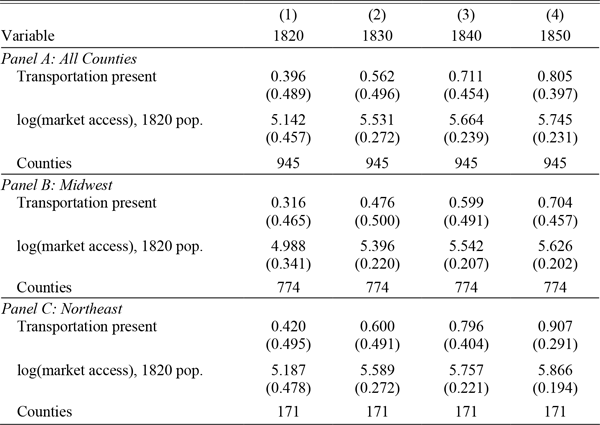
Table 1 summarizes the county-level measures of transportation linkage, divided by region and decadal year and weighted by population. There was a clear pattern of growth over time in the fraction of the population living in a county linked to the transportation network. In the entire sample region, less than 40 percent of the population lived in a county that was linked to the transportation network in 1820. By 1850, this fraction had risen to over 80 percent. The Northeast and the Midwest viewed separately exhibited similar patterns, although the population of the Northeast was consistently more linked than that of the Midwest.
SUMMARY STATISTICS FOR COUNTY-LEVEL DATA

Notes: The sample in Panel A includes all counties with no urban population in 1820. Panels B and C divide this sample by region. Means are presented with standard deviations in parentheses. Observations are weighted by population in each decade.
Source: See text.
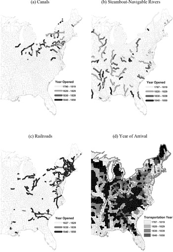
Figure 1 provides a graphical summary of the spread of transportation infrastructure over this period. Panels (a)–(c) show the spread of each mode of transportation. Panel (d) uses this information to determine the year that a county was first linked to the (nonwagon) transport network. It shows that the transportation network gradually spread inland. The sample period began with only the coasts and the counties bordering the major internal waterways being linked to the network, and it concluded with much of the interior being linked, particularly in the North.
SPREAD OF TRANSPORTATION INFRASTRUCTURE

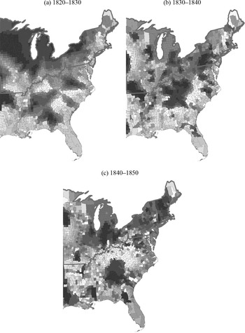
Market access is also summarized in Table 1. As with the linkage measure, this measure shows patterns of growth over the study period, and of greater market access in the Northeast than in the Midwest. The development of the market access measure over time and space is described graphically in Figure 2. This figure depicts the change in market access in each decade, darker shading indicating counties with greater increases.Footnote 27 It shows that, as intended, market access captures changes that transportation linkage does not. For instance, the counties in the sample region with the greatest increase in market access between 1820 and 1830 are those bordering the upper Mississippi and the Great Lakes, as well as those in western New York. These changes reflect the opening of the Erie Canal and of the upper Mississippi. Between 1830 and 1840, large increases are observed in central Pennsylvania and in Indiana and Ohio, reflecting canal construction. Finally, between 1840 and 1850, large increases are again observed in Indiana and Ohio, also reflecting canal construction.
CHANGES IN MARKET ACCESS BY DECADE

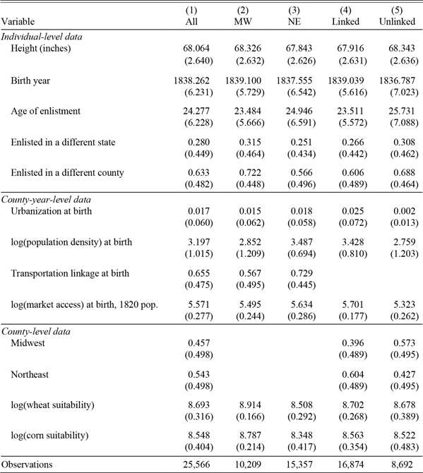
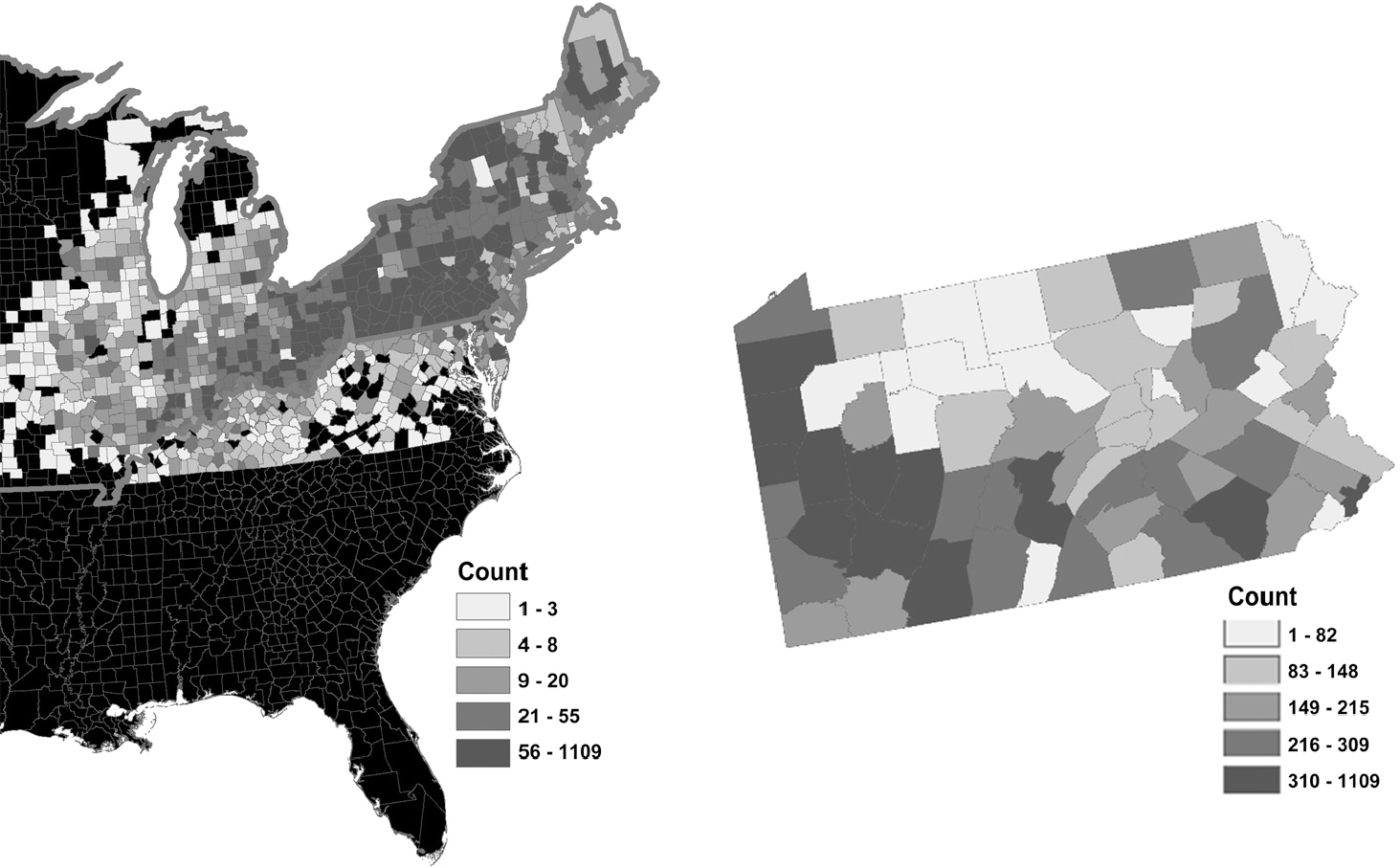
Table 2 provides summary statistics at the individual level for heights and for other variables for the complete sample and for various subsamples. Column (1) represents the benchmark sample of analysis—native-born white males whose counties of birth had no urban population in 1820. Columns (2) and (3) divide the sample by region, and Columns (4) and (5) divide the sample by whether the individual’s county of birth was linked or unlinked to the transportation network in the individual’s year of birth. A majority of the sample was born in the Northeast—a mechanical consequence of weighting the data to reflect state population in 1860. Figure 3 delves into the geographic distribution of data in further detail. It presents the number of individual height observations by county, separating Pennsylvania from the rest of the country. On the whole, the sample tends to draw from the more populous areas of the country. Importantly, it includes almost all counties in the Northeast and the Midwest.Footnote 28 Nonetheless, some counties are represented by only a small number of observations. To ensure that limited representation of some counties does not create spurious results, Online Appendix E repeats the main analysis limiting the sample either to the better represented states of New York and Pennsylvania or to counties with at least 100 observations, with similar results.
SUMMARY STATISTICS FOR INDIVIDUAL-LEVEL DATA

Notes: The sample includes all height observations of native-born white males born in the Northeast or Midwest in counties with no urban population in 1820. Means are presented with standard deviations in parentheses. Observations are weighted to correct for oversampling. Linked indicates individuals born in counties with a transport link in the birth year; unlinked denotes the opposite. MW denotes Midwest; NE denotes Northeast. The number of observations refers to the number of individuals in the sample with known height, year of enlistment, age of enlistment, and county of birth.
Source: See text.
NUMBER OF OBSERVATIONS BY COUNTY

Table 2 also shows that the benchmark sample was 68.1 inches tall on average, and Columns (2) and (3) reveal that the Northeast suffered a height disadvantage of about half an inch relative to the Midwest. A height disadvantage of about 0.4 inches is present for those born in transportation-linked counties relative to those whose birth counties were unlinked in the birth year.Footnote 29
There are also differences between regions and between linked and unlinked counties in measures of population concentration. Consistent with the expected effects of transportation linkage (and with a variety of endogeneity concerns), there is a considerable advantage in urbanization and population density at birth for individuals born in linked counties.Footnote 30 There is also an advantage in population density at birth for Northeasterners, though the level of urbanization at birth was similar for the Northeast and the Midwest (recall that any county with an urban population in 1820 is omitted). While there is a premium in agricultural suitability for the Midwest, there does not appear to be a meaningful difference in agricultural suitability of the birth county for individuals born in linked and unlinked counties.
Finally, about 27 percent of the sample enlisted in a state other than the state of birth (state of enlistment is determined by the state of the regiment in which an individual enlisted), while nearly 63 percent enlisted in a county other than the county of birth.Footnote 31 The probability of enlisting in a county or state other than that of birth was greater for Midwesterners but smaller for individuals born in counties linked to the transportation network.
Empirical Specification
The basic specification that I use to study the relationship between transportation and height is
 $$\matrix{ {{h_{ijt}} = {\gamma _t} + {\delta _a} + {\delta _e} + \beta {x_{jt}} + {\bf{z}}_j^\prime\tau + {\varepsilon _{ijt}}}. \cr }$$
In Equation (2), hijt is the height of individual i born in county j in year t, γt are birth cohort-specific intercepts, δa are indicators for each measurement age below 21 to address cases in which individuals are observed before reaching terminal height, δe are enlistment-year fixed effects designed to address the possibility of changing composition of military enlisters over the course of the Civil War,Footnote 32xjt is a measure of transportation linkage in the birth year (either the binary measure or the logarithm of market access), and zj is a vector of various county-level control variables to be introduced below.Footnote 33 I cluster standard errors throughout the analysis at the county level.Footnote 34 My initial analysis estimates this equation by ordinary least squares (OLS). This specification is comparable to that used by prior studies of the transportation-health relationship in the antebellum United States (especially Haines, Craig, and Weiss Reference Haines, Craig and Weiss2003).
This framework assumes that the effect of transportation on height is described fully by the relationship of terminal height with transportation linkage in the birth year. While previous studies suggest that conditions in the birth year are likely to be more important than in any other year of life (e.g., Steckel Reference Steckel1995; Woitek Reference Woitek2003), it is possible to determine the consequences of relaxing this assumption. I do this in Online Appendix B, where I find that transportation linkage around the year of birth is more strongly associated with terminal stature than is transportation linkage in other phases of life.
Although Equation (2) is useful in establishing a correlation, any relationship that it uncovers between transportation and height may be spurious. For instance, a particular county may have been densely populated or highly urbanized for some reason besides transportation linkage, such as a favorable geographic location. When transportation infrastructure was constructed, the fact that this county was already developed would make it more likely to become linked to the network.Footnote 35 Moreover, the sanitation consequences of population concentration might make this area unhealthy. This hypothetical relationship would produce a negative β in Specification (2) even if the true β were zero. Not all confounds must be in this direction. For instance, if better agricultural land attracted transport construction and raised incomes and health, a spurious positive β would arise.
The improved data available from Atack’s (Reference Atack2015, Reference Atack2016, Reference Atack2017) shape files and the advantages of market access as a measure of transport linkage enable me to address these endogeneity concerns. The panel structure of the transportation data enables me to augment Equation (2) with the addition of county fixed effects αj (requiring the omission of the county-specific controls zj) so that it becomes
 $$\matrix{ {{h_{ijt}} = {\alpha _j} + {\gamma _t} + {\delta _a} + {\delta _e} + \beta {x_{jt}} + {\varepsilon _{ijt}}}. \cr }$$
This specification captures time-invariant county characteristics (such as a favorable location), identifying the effect of transportation on height on the basis only of local changes.
A concern that remains in Equation (3) is that a force other than transportation that varies over time within a county might both affect health and attract transportation. For instance, a favorable location might only have become important as the economy grew. This concern would not be captured by the county fixed effects αj. One approach that I will use to address this concern is to include county-decade fixed effects rather than simply county fixed effects.Footnote 36 Another approach is made possible by the use of market access to measure transportation linkage. Specifically, I can estimate
 $$\matrix{ {{h_{ijt}} = {\alpha _j} + {\gamma _t} + {\delta _a} + {\delta _e} + \beta \log \left( {{\rm{M}}{{\rm{A}}_{jt}}} \right) + \pi {T_{jt}} + {\varepsilon _{ijt}}}, \cr }$$
where MAjt is market access computed as in Equation (1) and Tjt is a binary indicator of transportation linkage. The coefficient of interest in this equation is β. Based on the identification strategy used by Donaldson and Hornbeck (Reference Donaldson and Hornbeck2016) and Hornbeck and Rotemberg (Reference Hornbeck and Rotemberg2019), this specification identifies the effect of market access on height on the basis only of variations in market access induced by construction elsewhere in the network. That is, any endogeneity is likely to be captured by directly controlling for local transport linkage. The remaining variation in market access, which drives the estimate of β , is then relatively free of this endogeneity.
Online Appendix G presents an additional identification strategy, based on the straight-line instruments commonly used in the transport literature (e.g., Atack et al. Reference Atack, Bateman, Haines and Margo2010; Banerjee, Duflo, and Qian Reference Banerjee, Duflo and Qian2012; Ghani, Goswami, and Kerr Reference Ghani, Goswami and Kerr2016; Hornung Reference Hornung2015). In particular, I compute an alternative measure of market access based on the 1820 transport network augmented with canals built to connect major watersheds (i.e., the Atlantic, Great Lakes, and Mississippi) to one another and to major cities. I then use this alternative measure of market access to instrument for actual market access. This analysis, which also finds evidence of a negative effect of market access on height, provides supporting evidence based on an entirely different source of identifying variation.
THE EFFECT OF TRANSPORTATION ON HEIGHT
OLS Results
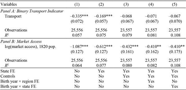
I begin the analysis by estimating Equation (2) by OLS using the binary indicator of transportation linkage as the regressor of interest. This estimation most closely matches that performed by Haines, Craig, and Weiss (Reference Haines, Craig and Weiss2003). Results of this estimation are presented in Panel A of Table 3. The regression of Column (1), which includes only birth-year indicators, age-of-measurement indicators, enlistment-year indicators, and no other controls, yields a negative and statistically significant relationship between transportation presence in the birth year and average stature. This relationship is robust to the inclusion of state fixed effects in Column (2), though this addition reduces the magnitude of the estimated coefficient by about half. This latter estimate indicates that individuals whose counties of birth had a transport link in their birth year were 0.17 inches shorter than those whose counties of birth were unlinked in their year of birth. This magnitude is large compared to the contemporaneous urban height penalty of 0.29 inches (Zimran Reference Zimran2019). It is also roughly comparable in magnitude to the estimates of Haines, Craig, and Weiss (Reference Haines, Craig and Weiss2003), whose benchmark results indicate that transportation linkage in the county of birth (though not necessarily in the year of birth) was associated with a height penalty of about 0.25 inches.
OLS REGRESSIONS

Significance levels: ***p < 0.01, **p < 0.05, *p < 0.1.
Notes: The dependent variable is height in inches. The sample includes individuals born in the Northeast or Midwest in counties with no urban population in 1820. All specifications include birth-year, measurement-age, and enlistment-year fixed effects. Standard errors are clustered at the county level. Observations are weighted to correct for oversampling. Controls are Herfindahl indices for 1840 calorie and protein production, third-degree polynomials in the logarithm of distance from New York and Cincinnati, as well as logs of the following variables: 1840 calorie and protein production, 1850 values of farms and capital in manufacturing, area, 1820 population, 1840 cattle and swine stocks, 1840 employment by sector, 1840 values of agricultural and manufacturing output, population in 1840, and population in 1850.
Source: See text.
In Column (3), I repeat the specification of Column (2) with the addition of a variety of county-level controls. Some of these control variables are those that Haines, Craig, and Weiss (Reference Haines, Craig and Weiss2003) include in their analysis—1840 calorie and protein production, Herfindahl indices for calorie and protein production, and 1850 values of farms and capital in manufacturing. I also add several other variables that may have impacted health. These include area and 1820 population (to capture population concentration in 1820), 1840 cattle and swine stocks, 1840 employment by sector, and values of agricultural and manufacturing output. All of these variables are included in logarithmic form, and I also include the logarithm of population in 1840 and 1850 in order to make the other measures effectively per capita. I also include third-degree polynomials in the logarithm of distance from New York and Cincinnati. These controls are intended to capture a variety of county characteristics, such as agricultural productivity, density, and geography, that might generate health differences even in the absence of a transport link. The post-1820 values are included with full recognition that their 1820 values would be preferable (later values may be bad controls). However, due to the limited data availability of the antebellum period, the inclusion of data on, for example, agricultural production is not possible prior to 1840, and I err on the side of controlling for the features that these measures capture rather than not doing so. For the main results, I will capture these characteristics with county fixed effects.
The inclusion of these controls in Column (3) reduces the magnitude of the estimated coefficient on transportation linkage and renders the estimated coefficient statistically insignificant. While the magnitude of the resultant coefficient is non-negligible, it is considerably smaller than the estimates of Columns (1) and (2). The addition in Column (4) of interactions of birth year and region fixed effects, or of the interactions of state and birth year fixed effects in Column (5), has little additional impact on the estimates.
One potential reason for the lack of a statistically significant relationship between transport and height in Columns (3)–(5) of Panel A of Table 3 is that the transport indicator captures only a limited amount of variation in linkage.Footnote 37 Besides the conceptual benefits of the market access measure, discussed above, it also has the technical benefit of providing more treatment variation in a setting where data are limited. Panel B of Table 3 repeats the analysis of Panel A but replaces the binary measure of linkage with the logarithm of market access as the explanatory variable of interest. Columns (1) and (2) estimate Equation (2) without the additional county-level controls, without and with the inclusion of state fixed effects, respectively. As was the case with the binary measure of transportation linkage, a large, negative, and statistically significant coefficient is present on the measure of transportation linkage and is nearly halved (but is otherwise robust) when state fixed effects are included. In particular, the estimates of Column (2), which include the state fixed effects, indicate that a one-standard-deviation increase in market access (0.28 log points, as shown in Table 2) is associated with a reduction in average height of 0.171 inches.
Columns (3)–(5) repeat this estimation, including the various county-level control variables and the region-by-birth year or state-by-birth year indicators. The addition of these controls to regressions of height on market access does not eliminate the statistical significance of the negative relationship between market access and height. Moreover, the impact of the inclusion of the controls on the magnitude of the coefficient is smaller than it was for the transport indicator. In particular, the estimates of Column (5), which includes the state-by-birth year indicators, imply that a one-standard-deviation increase in market access is associated with a decline in average stature of 0.115 inches, or about 1.7 times the implied impact of a transportation linkage in its analog in Panel A.
Fixed Effects Results
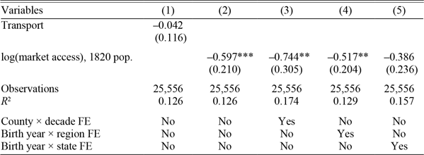
As discussed above, the results of Table 3 are potentially spurious. To begin addressing endogeneity concerns, Table 4 presents estimates of Equation (3), which includes county fixed effects. I begin in Column (1) by using the transport linkage indicator as the regressor of interest. Given the binary regressor, this coefficient can be interpreted as a generalized difference-in-differences coefficient. The estimated coefficient is –0.042, which is smaller than the estimates including controls in Table 3 and is statistically insignificant. Given the conceptual and technical limitations of the transport linkage indicator, as discussed above, the absence of a meaningful transport-health relationship using this regressor is not surprising.
COUNTY FIXED EFFECTS REGRESSIONS

Significance levels: ***p < 0.01, **p < 0.05, *p < 0.1.
Notes: The dependent variable is height in inches. The sample includes individuals born in the Northeast or Midwest in counties with no urban population in 1820. All specifications include birth-year, measurement-age, enlistment-year, and county fixed effects. Standard errors are clustered at the county level. Observations are weighted to correct for oversampling.
Source: See text.
Column (2) estimates the same specification with the logarithm of market access as the regressor of interest. This column reveals that the negative and statistically significant relationship between market access and height is robust to the inclusion of the county fixed effects, and thus to the concerns that they address over endogeneity. Moreover, at –0.597, the magnitude of the coefficient is comparable to the estimates of Table 3.
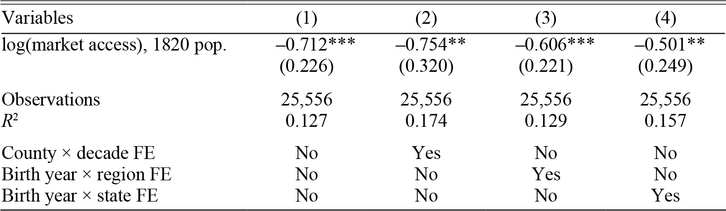
This result and its approximate magnitude are robust to the inclusion, in Column (3), of county-decade fixed effects in order to more flexibly address county-specific characteristics that may be time variant. Columns (4) and (5) supplement the county fixed effects with region- and state-by-birth year indicators, respectively. While the inclusion of these indicators reduces the magnitude of the estimated coefficients, and in the case of Column (5) it is reduced to the point of being marginally statistically insignificant (p = 0.102), the rough magnitude and sign of the coefficient is retained, supporting the conclusion that transportation improvements generated declines in stature-implied health.
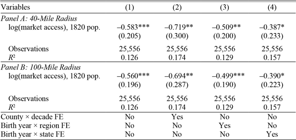
Table 5 investigates the extent to which the height-market access relationship uncovered in Table 4 is driven by connections to nearby or more distant counties. In particular, I adjust Equation (1) to compute market access as
 $${\widetilde{{\rm{MA}}}_{jt}} = {10^{ - 4}}\sum\limits_k {{p_k}} \tau _{jkt}^\theta 1\left\{ {{d_{jk}} \gt \bar d} \right\},$$
where djk is the distance between counties j and k, {ċ} is the indicator function, and  $\bar d$ is a cutoff value. I then re-estimate Equation (3) using this alternative measure of market access as the regressor of interest. Panel A of Table 5 uses a 40-mile cutoff, following Fogel’s (Reference Fogel1964) use of this distance as an important cutoff; Panel B uses a 100-mile cutoff. The results of Table 5 indicate that the impact of market access on height largely comes from the reduction of transport costs to more distant markets—the results are virtually identical to those of Table 4 even after replacing MAjt with
 ${{\widetilde{{\rm{MA}}}_{jt}}}$ computed as in Equation (5).
MARKET ACCESS OMITTING NEARBY COUNTIES

Significance levels: ***p < 0.01, **p < 0.05, *p < 0.1.
Notes: The dependent variable is height in inches. The sample includes individuals born in the Northeast or Midwest in counties with no urban population in 1820. All specifications include birth-year, measurement-age, enlistment-year, and county fixed effects. Panel A computes a county’s market access omitting counties within 40 miles. Panel B computes a county’s market access omitting counties within 100 miles. Standard errors are clustered at the county level. Observations are weighted to correct for oversampling.
Source: See text.
To further address potential endogeneity of transport linkage, I estimate Equation (4). By controlling directly for transport linkage, these specifications identify the effect of market access on height using only variation in linkage coming from construction elsewhere in the network, which is less likely to be endogenous to local development than is the directly-controlled-for local construction. Reassuringly, the negative effect of market access on height documented in Table 4 is made even stronger by the results of Table 6, which provide plausibly causal estimates consistent with this effect.Footnote 38 Overall, based on the results of Tables 4–6, I conclude that the data provide strong and robust evidence of a negative relationship between stature and market access in the county-year of birth.
COUNTY FIXED EFFECTS REGRESSIONS CONTROLLING FOR TRANSPORT LINKAGE

Significance levels: ***p < 0.01, **p < 0.05, *p < 0.1.
Notes: The dependent variable is height in inches. The sample includes individuals born in the Northeast or the Midwest in counties with no urban population in 1820. All specifications include birth-year, measurement-age, enlistment-year, and county fixed effects, as well as an indicator for having a transport link in the birth year in the county of birth. Standard errors are clustered at the county level. Observations are weighted to correct for oversampling.
Source: See text.
Having shown that transportation linkages had a deleterious impact on health in the antebellum period, these results provide an empirical basis for a potential explanation of the Antebellum Puzzle—that it was caused, in part, by the expansion of the transportation network in the antebellum period. This is the first evidence of an explanation for the Antebellum Puzzle with estimates that can plausibly be given a causal interpretation, and the first that relates declines in height to changes in local circumstances (by virtue of the county fixed effects included in the estimation).
How much of the deterioration in average stature can be attributed to the growth of the transportation network? The empirical pattern to be explained is a 0.82-inch decline in average stature that is present in the benchmark sample.Footnote 39 Table 1 shows that the logarithm of market access increased by 0.603 from 1820 to 1850. My preferred estimate of the effect of market access on height is given by Column (4) of Table 6, which uses the Donaldson and Hornbeck (Reference Donaldson and Hornbeck2016) and Hornbeck and Rotemberg (Reference Hornbeck and Rotemberg2019) method to address endogeneity and which includes the most conservative time trends.Footnote 40 Thus, the coefficient of –0.501 implies that changing market access can explain a decline in average stature of 0.30 inches, or 37 percent of the observed decline.
It is also possible that a negative relationship between market access in the county-year of birth and health as measured by adult stature may be the result of individuals leaving newly linked locations to move to less healthy urban environments, implying that the new transport linkages did not reduce the health of the place of birth but, instead, pushed individuals to move to other, less healthy locations. Alternatively, the results may be the product of less healthy individuals moving to newly linked areas and having children there who have lower adult stature. Neither of these cases would inhibit the interpretation of the results above as the causal effect of transportation linkages on the terminal heights of individuals born in an affected county-year; but, if these were the mechanisms by which the effect operated, the interpretation of the results as explaining an overall decline in average stature in the whole economy would be more tenuous. In Online Appendix H, I show that to the extent that it is possible to evaluate these mechanisms, they are not consistent with the data.
THE LOCAL DEVELOPMENT MECHANISM
As discussed above, there are at least three mechanisms by which market access may have negatively impacted stature-implied health—disease transmission, local development, and relative prices. Distinguishing between these various theoretical mechanisms is important in better understanding the effects of transportation, the causes of the antebellum decline in health, and, ultimately, the welfare effects of early modern economic growth in the United States. Unfortunately, the limited data availability for the antebellum United States makes it impossible to evaluate all of these possible mechanisms. But there are sufficient data to determine whether there is empirical support for the mechanism of transportation increasing population density, thereby decreasing health, which I call the local development mechanism.
A necessary condition for this mechanism to be valid is that there should be a positive impact of increased market access on population density. I test this by estimating the equation
 $$\log \left( {{y_{jt}}} \right) = {\alpha _j} + {\gamma _t} + \beta \log \left( {{\rm{M}}{{\rm{A}}_{jt}}} \right) + \pi {T_{jt}} + {\varepsilon _{jt}}$$
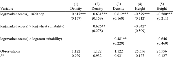
for years 1820–1850, where yjt is the population density of county j in year t, and the coefficient of interest is β . This is an adapted version of Equation (4), and like this equation, it identifies the effect of market access by observing the response to improvements in market access coming from construction elsewhere in the network. I present the results in Column (1) of Table 7. Following Atack et al. (Reference Atack, Bateman, Haines and Margo2010), I limit the sample to county-years in which counties had already achieved their 1860 boundaries so that results are not driven by changes in population density caused by changes in county boundaries. I weight observations according to the ratio of county population in each year to total population in that year. I find a large, positive, and statistically significant impact of market access on population density. The estimated coefficients imply that the increase in market access from 1820 to 1850 (0.603 in the data set with counties as the unit of observation, as shown in Table 1) is associated with a 0.372 log point increase in population density.
THE LOCAL DEVELOPMENT MECHANISM

Significance levels: ***p < 0.01, **p < 0.05, *p < 0.1.
Notes: The dependent variables are listed in the column headers. The sample in Columns (1)–(3) includes all county-years with borders fixed to 1860, with no urban population in 1820, and in the Midwest or Northeast. The sample in Columns (4) and (5) includes individuals born in the Northeast or Midwest in counties with no urban population in 1820. All specifications include year and county fixed effects and control for transportation linkage. Columns (4) and (5) also include measurement-age and enlistment-year fixed effects. Observations in Columns (1)–(3) are weighted by the ratio of county population in each year to total population in that year. Observations in Columns (4) and (5) are weighted to correct for oversampling. Standard errors are clustered at the county level.
Source: See text.
This result is an important piece of evidence in favor of the local development mechanism—it is well known that greater population density was associated with worse health (Floud et al. Reference Floud, Fogel, Harris and Hong2011), and it stands to reason that by inducing greater population density, transportation may have harmed health. More evidence, however, is available from heterogeneity in the effects of increased market access. I focus specifically on heterogeneity with respect to a county’s suitability for wheat and corn production.Footnote 41 Given the importance of these products in the long-distance trade that market access measures (as indicated, in part, by Table 5), I expect a greater increase in population density in response to increases in market access in more agriculturally suitable counties, as the benefits of greater market access are likely to be larger there.
Columns (2) and (3) of Table 7 test this prediction by interacting market access with the logarithm of a measure of a county’s average suitability for wheat or corn production (Food and Agriculture Organization 2002). The results are consistent with this prediction, revealing that the effects of market access on increasing population density were stronger in counties with greater agricultural suitability. I demean the measures of suitability so that, for example, the estimates of Column (2) can be interpreted as implying that a county with average wheat suitability experienced an increase in population density of 0.631 percent in response to a one percent increase in market access and that a county with wheat suitability one percent above the mean had a 0.626-percentage-point stronger reaction. Similar results are evident for corn suitability. Thus, counties with greater agricultural suitability tended to experience greater increases in population density in response to improvements in transport linkages, likely reflecting immigration of individuals seeking to establish farms. This view is further supported by Table A.4 in Online Appendix A, which shows an increase in the acreage devoted to farming in response to rising market access, with greater increases in counties with greater suitability for wheat and corn production.Footnote 42
This heterogeneity in the effect of market access on population provides an opportunity to test the local development mechanism. If population density increased more in response to rising market access in more agriculturally suitable counties, then average stature should have decreased more in response to rising market access in these counties.Footnote 43 To test this, I repeat the interaction approach in estimating Equation (4) in Columns (4) and (5) of Table 7, with height as the dependent variable. I find that, as predicted, the negative relationship of market access with stature was stronger in the more agriculturally suitable counties, though the interaction coefficients are only marginally statistically significant (p = 0.095 for wheat suitability and p = 0.159 for corn suitability).
Altogether, the results of Columns (2)–(5) of Table 7 indicate that in the counties where agricultural productivity caused population density to grow more in response to rises in market access, the effects of market access on reducing height were stronger. This is consistent with the contention that the effect of transportation on market access passed through the channel of increasing local development that, in a setting of poor sanitation and public health, worsened the local disease environment.
This evidence adds to the debate over the causes of the antebellum deterioration in health. As discussed above, the local development mechanism is a component of the disease explanation for the Antebellum Puzzle. By finding evidence consistent with this mechanism, I add to the evidentiary basis of the disease explanation.Footnote 44
CONCLUSION
Why did health in the United States deteriorate in the antebellum period, just as modern economic growth began? This is an important question of U.S. economic history—one that bears centrally on understanding the evolution of living standards on the American path to industrial leadership. Since this Antebellum Puzzle was first discovered by Fogel et al. (Reference Fogel, Engerman, Floud, Steckel, Trussell, Wachter, Margo, Sokoloff and Villaflor1979), economic historians have sought to explain why health deteriorated at the onset of modern economic growth, which should have improved it. But evidence as to possible answers to this question is limited. In this paper, I test whether the transportation improvements of the antebellum period contributed to the decline in average stature.
Specifically, I study the relationship between transportation and height in the antebellum United States using data on stature from the records of enlistments in the Union Army combined with GIS data on the development of the antebellum transportation network. I find evidence of a negative effect of market access on average stature that is large enough to explain 37 percent of the decline in average stature in my data. Evidence supporting such a relationship had previously been found (Cuff Reference Cuff2005; Haines, Craig, and Weiss Reference Haines, Craig and Weiss2003; Yoo Reference Yoo2012), but improvements in data availability (Atack Reference Atack2013) and methods for the study of transportation (Donaldson and Hornbeck Reference Donaldson and Hornbeck2016) enable me to provide plausibly causal estimates where only suggestive correlations had previously been available. I also go beyond this existing research by providing evidence consistent with the contention that a mechanism for this effect was the role of transportation in increasing population density, which would have led to a deterioration in the epidemiological environment in a period of poor sanitation technology.
This paper helps to better understand the impacts of transportation infrastructure construction in the historical United States, and in developing countries more generally. In such settings, the beneficial effects of transportation improvements for economic development are well known (Bogart Reference Bogart, Diebolt and Haupert2018; Donaldson Reference Donaldson2015). Less is known, however, about the impact of transportation on health, where the theoretical impact is ambiguous and only a small number of empirical investigations exist to study this impact in specific settings (Burgess and Donaldson Reference Burgess and Donaldson2012; Tang Reference Tang2017). As a result, this paper sheds light on an aspect of the literature that is only beginning to come into focus.
On the whole, this paper provides an interesting and important warning. The Antebellum Puzzle cautions that the early phases of modern economic growth may not be unambiguously welfare-improving. The results of this paper show that infrastructure improvements with well-known economic benefits may also have an unintended negative impact on at least some aspect of welfare and, therefore, may also not be unambiguously welfare-improving.