1. Introduction
Droplets constitute an integral part of a wide variety of natural and industrial processes, including pharmaceuticals (Zhang, Chan & Leong Reference Zhang, Chan and Leong2013; Iqbal et al. Reference Iqbal, Zafar, Fessi and Elaissari2015), food (Kralova & Sjöblom Reference Kralova and Sjöblom2009; Dickinson Reference Dickinson2011; Lamba, Sathish & Sabikhi Reference Lamba, Sathish and Sabikhi2015), cosmetics (Varvaresou & Iakovou Reference Varvaresou and Iakovou2015; Venkataramani, Tsulaia & Amin Reference Venkataramani, Tsulaia and Amin2020), crude-oil processing (Frising, Noïk & Dalmazzone Reference Frising, Noïk and Dalmazzone2006; Bera & Mandal Reference Bera and Mandal2015; Abdulredha et al. Reference Abdulredha, Hussain, Abdullah and Hong2022), among many others. Of late, somewhat more sophisticated applications have also emerged, especially in areas related to micro- and millifluidic devices (Teh et al. Reference Teh, Lin, Hung and Lee2008). Indeed, droplets are now routinely used for encapsulating specific cells and particles in miniaturised platforms (Stone, Stroock & Ajdari Reference Stone, Stroock and Ajdari2004; Vollenbroek et al. Reference Vollenbroek, Nieuwelink, Bomer, Tiggelaar, van den Berg, Weckhuysen and Odijk2023) for the purposes of monitoring and analysis (Köster et al. Reference Köster2008; Li et al. Reference Li, Liu, Zhuang and Goda2021). For instance, droplet-based flow cytometry (McKinnon Reference McKinnon2018) is now a standard tool in a biochemist’s toolbox, which heavily relies upon encapsulating cells using small drops. This facilitates single-cell analysis (Li et al. Reference Li, Liu, Zhuang and Goda2021) and industrial enzyme production (Yuan et al. Reference Yuan, Tu, Tong, Lin, Zhang and Wang2022), and thus, holds significant promise for drug discovery as well as other biomedical applications (Yin & Marshall Reference Yin and Marshall2012). Furthermore, droplets also serve as versatile microreactors by enabling efficient mixing of reagents, and have been used as such for nanoparticle synthesis (Nightingale et al. Reference Nightingale, Krishnadasan, Berhanu, Niu, Drury, McIntyre, Valsami-Jones and DeMello2011; Zhang et al. Reference Zhang, Wang, Tong and Xia2014), analysis of reaction kinetics related to food digestion and nutrient absorption (Schroen et al. Reference Schroen, Berton-Carabin, Renard, Marquis, Boire, Cochereau, Amine and Marze2021), and medical diagnostics and therapeutics (Kaushik, Hsieh & Wang Reference Kaushik, Hsieh and Wang2018; Agnihotri et al. Reference Agnihotri, Ugolini, Sullivan, Yang, De Ganzó, Lim and Konry2022; Aubry, Lee & Lu Reference Aubry, Lee and Lu2023). In all these applications, precise monitoring and control of droplet trajectories in narrow confinements become indispensable.
It has long been established that the kinetics of a drop is significantly influenced by surface-active agents (surfactants), which are routinely added (and sometimes are naturally present) in multiphase systems for stabilising them (Baret Reference Baret2012). Most surfactants are soluble in the continuous phase and are adsorbed onto the suspended droplets’ interfaces, thus forming Gibbs monolayers. This causes the interfacial tension to reduce, and the extent of this reduction depends on the precise interfacial surfactant concentration. As the ensuing background flow transports the surfactants, their distribution becomes uneven, resulting in surface tension gradients and subsequently Marangoni stresses (Stone & Leal Reference Stone and Leal1990; Leal Reference Leal2007). The interaction between these stresses and the imposed flow are often quite intricate because of the nonlinear coupling between flow and surfactant transport and, hence, their impact on the drop’s motion may also be far ranging. In particular, inside narrow confinements, asymmetric Marangoni stresses have been shown (Hanna & Vlahovska Reference Hanna and Vlahovska2010; Pak et al. Reference Pak, Feng and Stone2014; Das et al. Reference Das, Mandal, Som and Chakraborty2017, Reference Das, Mandal and Chakraborty2018; Ahmed et al. Reference Ahmed, Izbassarov, Lu, Tryggvason, Muradoglu and Tammisola2020) to instigate cross-stream migration of droplets towards the channel centreline, which underscores their capability towards controlling droplet trajectories.
In many practical applications (such as the stabilisation of emulsions, cytometry, oil recovery, and of late, in active drops; see, e.g. Maass et al. Reference Maass, Krüger, Herminghaus and Bahr2016; Lippera et al. Reference Lippera, Morozov, Benzaquen and Michelin2020; Dwivedi, Pillai & Mangal Reference Dwivedi, Pillai and Mangal2022; Michelin Reference Michelin2023) a relatively high concentration of surfactants is used to maximise their impact. When the concentration exceeds the critical micelle concentration (CMC), the excess individual surfactant molecules, called monomers, undergo spontaneous self-aggregation. As a result, depending on the geometry and the intermolecular interactions between the monomers, they may either completely phase separate or form finite-sized aggregates called micelles (Israelachvili Reference Israelachvili2011). The micelles often act as surfactant reservoirs, releasing or consuming free monomers near a droplet interface (Stebe, Lin & Maldarelli Reference Stebe, Lin and Maldarelli1991; Stebe & Maldarelli Reference Stebe and Maldarelli1994), and hence, are expected to influence the flow around the drop. In particular, it has been shown (Lucassen Reference Lucassen1975; Stebe et al. Reference Stebe, Lin and Maldarelli1991; Langevin Reference Langevin2014; Manikantan & Squires Reference Manikantan and Squires2020) that the formation and breakup of micelles help sustain a nearly uniform monomer concentration in the bulk, which, in turn, affects the adsorption–desorption at the droplet interface. This can suppress the Marangoni stresses leading to interfacial remobilisation, thereby affecting how the droplets move.
Despite their prevalence, theoretical/numerical investigations on droplet motion in the presence of high concentrations of surfactants, especially those beyond the CMC, are relatively scarce in the literature. Some recent studies mainly focus on instabilities associated with planar interfaces in the presence of micelles, and assume that they do not directly interact with the surfactants adsorbed at the interface (Craster, Matar & Papageorgiou Reference Craster, Matar and Papageorgiou2009; Kalogirou & Blyth Reference Kalogirou and Blyth2019, Reference Kalogirou and Blyth2020). In contrast, Morozov (Reference Morozov2020) has explored self-propelling active drops, where micelles do interact with the droplet interface, forming swollen micelles that absorb and transport small fractions of the droplet phase – a mechanism popularly known as solubilisation. On the other hand, most prior studies (Janssen & Anderson Reference Janssen and Anderson2008; Hanna & Vlahovska Reference Hanna and Vlahovska2010; Sharanya et al. Reference Sharanya, Sekhar and Rohde2018, Reference Sharanya, Sekhar and Rohde2019; Panigrahi et al. Reference Panigrahi, Santra, Banuprasad, Das and Chakraborty2021) only explore the motion and possible cross-stream migration of passive drops being advected in narrow confinements in the presence of bulk-insoluble surfactants. The relatively few who do account for bulk solubility (Luo, Shang & Bai Reference Luo, Shang and Bai2019; Ahmed et al. Reference Ahmed, Izbassarov, Lu, Tryggvason, Muradoglu and Tammisola2020) have largely ignored the role of micelles and only probed the space of low concentrations. Therefore, the mechanics of micelle formation in bulk-soluble surfactants with high concentrations, their interactions with a drop suspended in an external flow and their subsequent impact on the precise trajectory of the drop remains an important open question with significant practical relevance.
Here, we attempt to address the above open question by examining the role of a highly concentrated surfactant solution as the continuous phase with concentrations exceeding the CMC, in governing the trajectory of a small drop. We consider the drop to be suspended in an unbounded Poiseuille flow, which is tantamount to ignoring the impact of the confinement walls. We construct a semi-analytical-cum-numerical framework to solve the flow and the surfactant concentrations around the drop along with its trajectory. The micelles are assumed to be monodisperse, while the transport of surfactants (both monomers and micelles) are characterised by arbitrary Péclet numbers (
 $Pe_s,\;Pe_b$
and
 $Pe_m$
, defined later), with an arbitrarily strong coupling between bulk and interfacial transport of monomers – characterised by the bulk interaction parameter
 $\omega$
(defined later) (Jadhav, Mandal & Ghosh Reference Jadhav, Mandal and Ghosh2024).
Our results reveal that the droplet undergoes cross-stream migration towards the channel centre – indeed, this has been known in the literature (Hanna & Vlahovska Reference Hanna and Vlahovska2010) for bulk-insoluble surfactants. The rate of this migration strongly depends on the bulk surfactant concentration and its precise impact hinges on the sensitivity of the interfacial tension to the surfactant molecules (characterised by the Marangoni number,
 $Ma$
). Beyond the CMC, however, the bulk monomer concentration reaches an upper bound, which restricts the influence of any further increase in the bulk concentration on the cross-stream migration of the drop. We further establish that increased adsorption–desorption between the interface and the bulk slows down the cross-stream migration, whereas a stronger coupling between interfacial and bulk transport facilitates the same.
The remainder of this paper is arranged as follows. Section 2 provides an outline of the physical system under consideration, the key assumptions, the characteristic scales and the important non-dimensional numbers. In § 3 (accompanied by Appendix A) we present the governing equations, the boundary conditions and the general semi-analytical framework for determining the drop’s trajectory and the associated concentration fields, along with a brief outline of the solution methodology. Section 4 along with Appendix B showcase the detailed results for the surfactant concentration distribution, parametric studies and droplet trajectories. Conclusions are drawn in § 5. Finally, in Appendix C the detailed formulation for the Frumkin isotherm, which incorporates non-ideal surfactant behaviour, is presented.
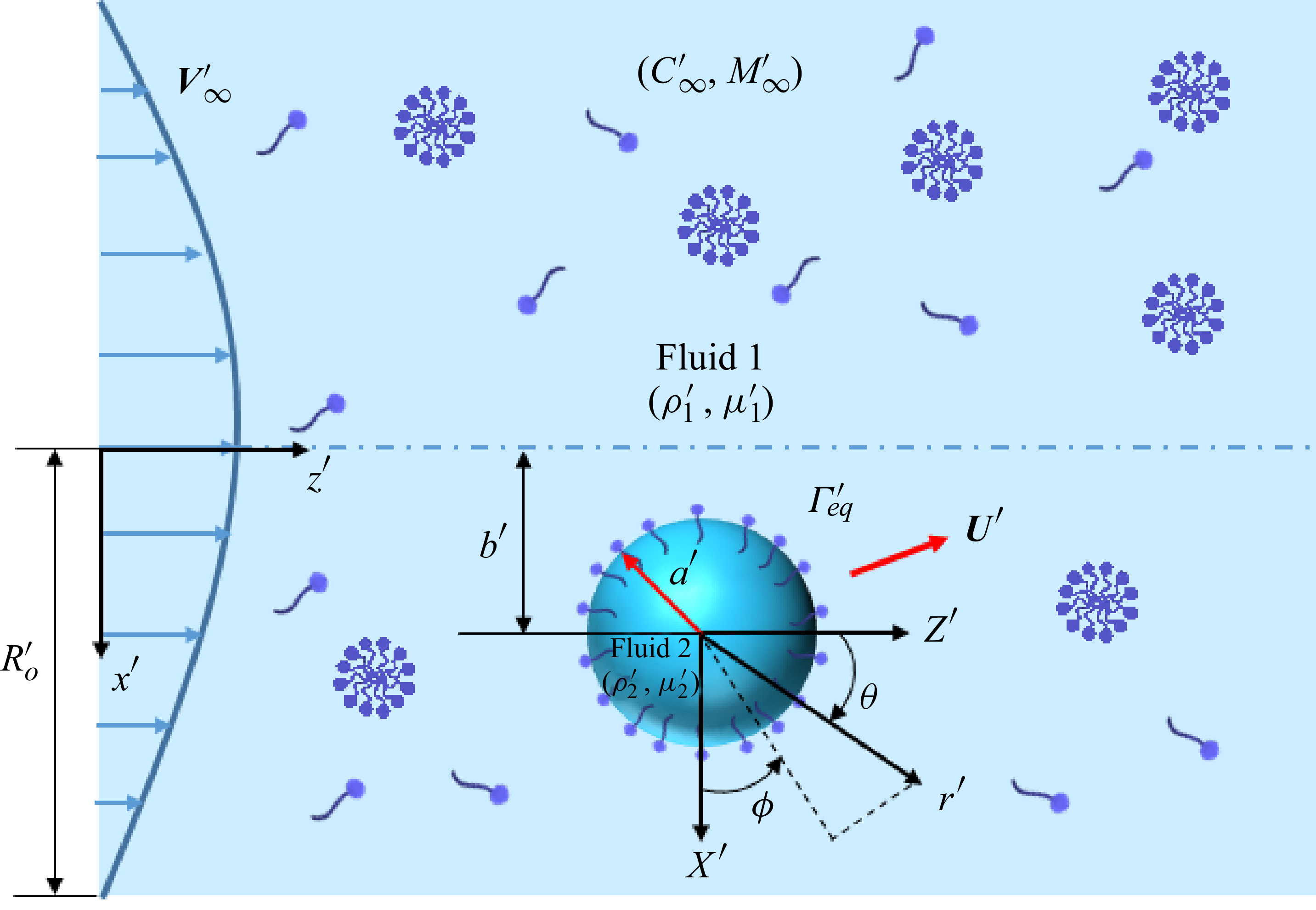
Schematic of a neutrally buoyant spherical drop of radius
 $a^{\prime}$
moving with velocity
 $\boldsymbol{U}^{\prime}$
in a background cylindrical Poiseuille flow of velocity
 $\boldsymbol{V}^{\prime}_{\infty}$
. The carrier phase (fluid 1) and the droplet (fluid 2) have density
 $\rho ^{\prime}_{1}$
and
 $\rho ^{\prime}_{2}$
, and viscosity
 $\mu ^{\prime}_{1}$
and
 $\mu ^{\prime}_{2}$
, respectively. Surfactant monomers and micelles are present in fluid 1 with far-field concentrations
 $C^{\prime}_{\infty}$
and
 $M^{\prime}_{\infty}$
, respectively. The total bulk concentration is
 $C^{\prime}_t = C^{\prime}_{\infty} + N M^{\prime}_{\infty}$
,
 $N$
being the aggregation number. The monomers are adsorbed from the bulk at the droplet interface to form a monolayer therein, with concentration
 $\varGamma ^{\prime}$
. The surface tension of the clean drop (
 $\sigma ^{\prime}_{s}$
) is reduced by the surfactants (
 $\sigma ^{\prime}(\varGamma ^{\prime})\lt \sigma ^{\prime}_{s}$
). A Cartesian coordinate system (
 $X^{\prime},Y^{\prime},Z^{\prime}$
) is attached to the drop centre, located at a cross-stream distance
 $b^{\prime}(t^{\prime})$
from the flow centreline. A spherical coordinate system (
 $r^{\prime},\theta ,\phi$
) is also attached to the drop centre. A fixed Cartesian coordinate system (
 $x^{\prime},y^{\prime},z^{\prime}$
) has also been shown, which tracks the overall motion of the drop.

2. The problem statement
2.1. Physical description of the system
Figure 1 illustrates the schematic representation of the physical system under consideration. We consider a spherical droplet of radius
 $a^{\prime}$
, moving with velocity
 $\boldsymbol{U}^{\prime}(t^{\prime})$
(a priori unknown) in an unbounded cylindrical Poiseuille flow. In a spherical coordinate (
 $r^{\prime},\theta ,\phi$
) attached to the droplet centre (see figure 1), this velocity field may be expressed as
 $\boldsymbol{V}^{\prime}_\infty = U^{\prime}_0[1-(b^{\prime}/R^{\prime}_0)^2 - r'^2\sin ^2{\theta }/R'^2_0 - 2r'b'\sin {\theta }\cos {\phi }/R'^2_o]\hat {\boldsymbol{e}}_z$
, where
 $U^{\prime}_0$
is the maximum centreline (by enforcing
 $b^{\prime} = 0$
) velocity,
 $R^{\prime}_0$
is the so-called cylinder radius and
 $b^{\prime}$
is the cross-stream distance of the drop from the centreline. The carrier phase (fluid 1) has density
 $\rho ^{\prime}_{1}$
and viscosity
 $\mu ^{\prime}_{1}$
, while the droplet phase (fluid 2) has density
 $\rho ^{\prime}_{2}$
and viscosity
 $\mu ^{\prime}_{2}$
. Surfactants at high concentrations (
 $\gt$
CMC) are present in the continuous phase, which may lead to the simultaneous existence of monomers and micelles in equilibrium. Their respective diffusivities are given by
 $D^{\prime}_b$
and
 $D^{\prime}_m$
, while their far-field equilibrium concentrations are (uniform)
 $C^{\prime}_{\infty}$
and
 $M^{\prime}_{\infty}$
, respectively. Each micelle is assumed to be an aggregate of
 $N$
monomers – this is called the aggregation number; the total bulk concentration of surfactants thus becomes
 $C^{\prime}_t = C^{\prime}_{\infty} + N M^{\prime}_{\infty}$
. For simplicity, we assume the micelles to be monodisperse, i.e. all micelles have the same aggregation number (
 $N$
), which is also independent of the total bulk concentration. Indeed, this condition is approximately satisfied for spherical micelles (such as those formed by sodium dodecyl sulphate) (Israelachvili Reference Israelachvili2011), although micelles with different geometries, such as rod-like or cylindrical ones show highly polydisperse aggregation numbers, which also depend on the bulk concentration. The formation and breakup of micelles are usually treated as an
 $N$
th-order reaction kinetics (Israelachvili Reference Israelachvili2011), with respective rate constants taken as
 $k^{\prime}_m$
and
 $k^{\prime}_b$
.
Bulk monomers also get adsorbed (and desorbed) at the droplet interface to form Gibbs monolayers, wherein the interfacial concentration is
 $\varGamma '$
(equilibrium value is
 $\varGamma ^{\prime}_{eq}$
). These interfacial surfactants get transported along the interface with surface diffusivity
 $D^{\prime}_{s}$
, while they also lower the surface tension as
 $\sigma '(\varGamma ')\lt \sigma ^{\prime}_{s}$
, where
 $\sigma ^{\prime}_{s}$
is the tension experienced by a clean (surfactant-free) interface. We take
 $k^{\prime}_a$
and
 $k^{\prime}_d$
respectively as the adsorption and desorption rate constants between the interface and the bulk. A Cartesian coordinate system (
 $X^{\prime},Y^{\prime},Z^{\prime}$
) may be attached to the drop’s centre, while another one fixed with the laboratory frame (
 $x^{\prime},y^{\prime},z^{\prime}$
) may also be set up as shown in figure 1, to track the overall movement of the drop.
2.2. The characteristic scales and the key assumptions
Hereon in the rest of the paper we use non-dimensional variables, unless otherwise mentioned. The non-dimensional version of any variable, say,
 $\mathcal{A}'$
is defined as
 $\mathcal{A} = \mathcal{A}'/\mathcal{A}_c$
, where
 $\mathcal{A}_c$
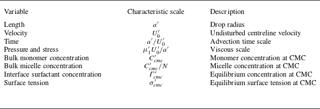
is the characteristic scale of the said variable. Table 1 lists the characteristic scales chosen in this paper. While the choice of characteristic scales for length, velocity and time are straightforward, the scale for the bulk monomer concentration is chosen as the CMC (
 $C^{\prime}_{\textit{cmc}}$
– see the discussion ahead) and that for the micelles (when they are present) is chosen as
 $C^{\prime}_{\textit{cmc}}/N$
. This also helps us pin down the characteristic interfacial surfactant concentration and the surface tension respectively to
 $\varGamma ^{\prime}_{\textit{cmc}}$
and
 $\sigma ^{\prime}_{\textit{cmc}}$
, which correspond to their equilibrium values (
 $\varGamma ^{\prime}_{eq}$
and
 $\sigma '(\varGamma ^{\prime}_{eq})$
) when the total bulk concentration is the same as the CMC (
 $C^{\prime}_t = C_{\textit{cmc}}$
).
Characteristic scales chosen for pertinent variables.

As we adopt a semi-analytical approach, a few assumptions become necessary. We have restricted the number of assumptions to a minimum and they are outlined as follows. (i) The flow is assumed to be viscosity-dominated and quasi-steady on the basis of a small Reynolds number (
 ${Re} = \rho ^{\prime}_1U^{\prime}_0a'/\mu ^{\prime}_1 \ll 1$
) and unit Strouhal number (
 $St = t_cU^{\prime}_0/a' = 1$
) (Leal Reference Leal2007). (ii) We shall assume that the drop remains spherical during the course of its motion on the basis of a small capillary number (
 $Ca = \mu ^{\prime}_1U^{\prime}_0/\sigma ^{\prime}_{\textit{cmc}} \ll 1$
) (Hanna & Vlahovska Reference Hanna and Vlahovska2010) – this is indeed a reasonable assumption and we justify it in the forthcoming subsection. (iii) We assume no direct interactions between the micelles and the interfacial surfactants. In the limited number of studies that do consider coupling between the transport of micelles and fluid flow, this assumption has been routinely enforced (Kalogirou & Blyth Reference Kalogirou and Blyth2019). However, we do emphasise that any additional interactions between the interfacial surfactants and the micelles (such as those due to solubilisation) may be seamlessly integrated within our framework, albeit at the expense of higher computational costs. (iv) For simplicity, in the main paper, we assume that the adsorption–desorption of monomers onto the interface follow the ideal gas isotherm. This holds true when the surfactant molecules are point-like and non-interacting (Manikantan & Squires Reference Manikantan and Squires2020). As a consequence, surface tension varies linearly with interfacial surfactant concentration as
 $\sigma ' = \sigma ^{\prime}_s - RT'\varGamma '$
, where
 $T'$
is the absolute temperature and
 $R$
is the universal gas constant. Furthermore, the net adsorption flux between the interface and the bulk takes the following simple form:
 $J^{\prime}_b = k^{\prime}_aC'-k^{\prime}_d\varGamma '$
(Manikantan & Squires Reference Manikantan and Squires2020). In a more general scenario, the surfactant molecules interact with each other, and are of finite size, which limits the maximum number of such molecules on an interface. These ‘non-ideal’ features become especially vital at high concentrations (
 $C^{\prime}_t \geqslant C^{\prime}_{\textit{cmc}}$
) and are nicely captured by the well-known Frumkin isotherm (Manikantan & Squires Reference Manikantan and Squires2020), although adapting it will enhance the complexity of the theory as well as the required computations. Nevertheless, we have also incorporated the Frumkin isotherm within our framework, the detailed formulation for which has been included in Appendix C. (v) Any excess rheological stresses (such as those given by the Boussinesq–Scriven model) arising from surfactants at the interface (Dandekar & Ardekani Reference Dandekar and Ardekani2020) are ignored. (vi) Finally, it is assumed that the channel walls play no role, which entails
 $a'/R^{\prime}_0 \ll 1$
.
The net micelle formation rate from the aggregation of
 $N$
monomers reads (Danov et al. Reference Danov, Vlahovska, Horozov, Dushkin, Kralchevsky, Mehreteab and Broze1996; Israelachvili Reference Israelachvili2011; Kalogirou & Blyth Reference Kalogirou and Blyth2020)
 $J^{\prime}_m = k^{\prime}_b C'^N - k^{\prime}_m M'$
. Far away from the drop, the monomers and the micelles are in equilibrium so that
 $J^{\prime}_m = 0$
. It then follows that in this region,
 $M^{\prime}_{\infty } = k^{\prime}_b C'^{N}_{\infty }/k^{\prime}_m$
, and the total bulk concentration becomes
 $C^{\prime}_t = C^{\prime}_{\infty} + N k^{\prime}_b C'^{N}_{\infty }/k^{\prime}_m$
. A little bit of algebra then shows that the micelle formation kick starts when
 $C^{\prime}_t$
exceeds a minimum threshold, given by
 $C^{\prime}_{\textit{cmc}} = (k^{\prime}_m/N k^{\prime}_b)^{1/(N-1)}$
– the CMC, which is now expressible in terms of the rate constants (Kalogirou & Blyth Reference Kalogirou and Blyth2020) and provides a natural choice for the characteristic concentration. It then follows from the expression for
 $J^{\prime}_b$
mentioned earlier that with
 $C^{\prime}_t = C^{\prime}_{\textit{cmc}}$
, the equilibrium interfacial concentration becomes
 $\varGamma ^{\prime}_{\textit{cmc}} = k^{\prime}_aC^{\prime}_{\textit{cmc}}/k^{\prime}_d$
– this provides a natural choice for the characteristic value of
 $\varGamma '$
.
2.3. The non-dimensional numbers
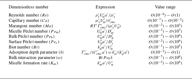
Upon enforcing the non-dimensionalisation scheme discussed in § 2.2, several important non-dimensional numbers emerge that are listed in table 2, along with their possible range of values. These have been computed based on a wide range of possible values of the underlying quantities (such as drop radius, centreline velocity, etc.), details of which are given in the caption. It is important to note that although
 ${Re} \ll 1$
,
 $Pe_m, Pe_b$
and
 $Pe_s$
may still be
 $O(1)$
or larger because the molecular diffusivities of monomers and micelles (
 $D'$
) are usually significantly smaller than the kinematic viscosities of various liquids that are used as the continuous phase. We further note that
 $Ca \ll 1$
, which supports assumption (ii) (negligible deformation) laid out in § 2.2. Indeed prior experiments (Santra et al. Reference Santra, Das, Das and Chakraborty2018) do reveal that surfactant-laden drops remain nearly spherical while undergoing cross-stream migration in a confined flow.
Key dimensionless numbers with their range of values. The following values have been chosen for the various characteristic scales:
 $a'\sim O(10^{-6}) - O(10^{-3})$
m,
 $U^{\prime}_0 \sim O(10^{-6}) - O(10^{-3})$
m s−1,
 $D^{\prime}_m$
and
 $D^{\prime}_b\sim O(10^{-9}) - O(10^{-11})$
m
 $^2$
s−1,
 $D^{\prime}_s\sim O(10^{-10})$
m
 $^2$
s−1,
 $\sigma ^{\prime}_{\textit{cmc}} \sim 10^{-2}$
N m−1,
 $\mu ^{\prime}_1\sim O(10^{-3}) - O(10^{-1})$
Pa s. Data taken from Chang & Franses (Reference Chang and Franses1995), Ferri & Stebe (Reference Ferri and Stebe2000), Kumar et al. (Reference Kumar, Priyadharsini, Prameela and Mandal2011), Kalogirou & Blyth (Reference Kalogirou and Blyth2020).

Schematic showing the role played by the various dimensionless numbers listed in table 2. (a) The micelle Péclet number (
 $Pe_m$
), the bulk Péclet number (
 $Pe_b$
), the surface Péclet number (
 $Pe_s$
) and the Biot number (
 $Bi$
) respectively contribute to the micelle, monomer and interfacial transport and the adsorption–desorption process. (b) The Marangoni number (
 $Ma$
) is associated with the surface tension gradient; adsorption depth (
 $\delta$
) is related to the rate of adsorption from the bulk. The micelle formation rate (
 $K_m$
) indicates how fast micelles form or dissociate. Panels (a) and (b) are adapted from Jadhav et al. (Reference Jadhav, Mandal and Ghosh2024). (c) Plot of equilibrium bulk monomer concentration (
 $C_{\infty }$
) and micelle concentration (
 $M_{\infty }$
) versus the total bulk concentration
 $C_t = C_{\infty } + M_{\infty } = C_{\infty } + C_{\infty }^N$
for aggregation number
 $N=100$
.

Figure 2 depicts the physical mechanisms that depend on some of the dimensionless parameters shown in table 2. While the physical significance of the various Péclet, Reynolds and capillary numbers are straightforward, we shall focus on the following key parameters. (a) The Marangoni number (
 $Ma$
), which indicates how sensitive the surface tension (
 $\sigma$
) is to the interfacial surfactant concentrations (
 $\varGamma$
) – see panel (b). (b) The Biot number (
 $Bi$
– see panel a), which is the ratio of the advective time scale (
 $t^{\prime}_a \sim a'/U^{\prime}_0$
) and the desorption time scale (
 $1/k^{\prime}_d$
);
 $Bi = 0$
signifies the insoluble surfactant limit. (c) The bulk interaction parameter (
 $\omega = Bi Pe_b \delta$
), which is the ratio of the time scales of the bulk diffusion of monomers (
 $\sim \delta ' a'/D^{\prime}_b$
) to the time scale of desorption from the interface; this parameter essentially dictates the extent to which the interfacial transport of surfactants influence the bulk transport (Jadhav et al. Reference Jadhav, Mandal and Ghosh2024). Here
 $\omega = 0$
signifies the decoupled limit due to infinitely fast bulk diffusion (Jadhav et al. Reference Jadhav, Mandal and Ghosh2024). Note that the definition of
 $\omega$
includes the adsorption depth
 $\delta$
, which indicates the extent of the region close to the interface where the monomer concentration gets depleted – see panel (b) for an illustration. (d) Finally, the micelle formation rate constant (
 $K_m$
) is another key parameter, which represents the time scale of the formation and breakup of micelles – we discuss more on this in § 3.1.2.
Figure 2(c) shows the variation of the (equilibrium) far-field monomer (
 $C_{\infty }$
) and micelle (
 $M_{\infty }$
) concentrations as the total bulk concentration
 $C_t= C_{\infty } + M_{\infty } = C_{\infty } + C_{\infty }^N$
(
 $0.1 \leqslant C_t \leqslant 3$
) is varied. The aggregation number has been taken as
 $N = 100$
. It is evident that for
 $C_t \lt C_{\textit{cmc}} = 1$
, only monomers are present in the continuous phase. On the other hand, micelle formation begins only when
 $C_t \gt 1$
, i.e. when
 $C_t$
exceeds the CMC, and concomitantly, the monomer concentration then plateaus at
 $C_{\infty } = 1$
. The above features of self-aggregation when the bulk concentration goes beyond the CMC is thus intrinsic to the
 $N$
th-order kinetics of micelle formation described at the end of § 2.2.
3. Analysis of droplet motion
3.1. Dimensionless governing equations and boundary conditions
3.1.1. Mass and momentum conservation equations
For brevity, we directly begin with dimensionless variables and equations, expressed in the reference frame attached to the drop. The flow in the
 $i$
th fluid (
 $i=1,2$
) satisfies the continuity and Stokes equations,
 \begin{equation} \boldsymbol{\nabla }\boldsymbol{\cdot }\boldsymbol{u}_i = 0, \quad \lambda _i{\nabla} ^2\boldsymbol{u}_i = \boldsymbol{\nabla } p_i, \end{equation}
where,
 $\boldsymbol{u},p$
are the velocity and pressure fields, respectively, and
 $\lambda _i = \mu ^{\prime}_i/\mu ^{\prime}_1$
is the viscosity ratio, with
 $\lambda _1 = 1$
and
 $\lambda _2 = \mu ^{\prime}_2/\mu ^{\prime}_1 = \lambda$
. These equations are subject to the far-field condition
 $\boldsymbol{u}_1\rightarrow \boldsymbol{u}_{\infty } = \boldsymbol{V}_{\infty } - \boldsymbol{U}$
,
 $p_1\rightarrow p_{\infty }$
as
 $r \rightarrow \infty$
and the boundedness condition,
 $|\boldsymbol{u}_2|\lt \infty , |p_2|\lt \infty$
, inside the drop. Here,
 $p_\infty$
is the pressure field associated with the imposed velocity field
 $\boldsymbol{V}_\infty$
. The boundary conditions at the drop interface are the continuity of velocity, no penetration and stress balance, which respectively take the following forms (Leal Reference Leal2007):
 \begin{align} \boldsymbol{I}_s\boldsymbol{\cdot }\boldsymbol{u}_1 & = \boldsymbol{I}_s\boldsymbol{\cdot }\boldsymbol{u}_2, \end{align}
 \begin{align} \boldsymbol{u}_1\boldsymbol{\cdot } \hat {\boldsymbol{n}} = & \boldsymbol{u}_2\boldsymbol{\cdot } \hat {\boldsymbol{n}} = 0, \end{align}
 \begin{align} (\boldsymbol{\tau }_1 - \boldsymbol{\tau }_2) \boldsymbol{\cdot } \hat {\boldsymbol{n}} = & \frac {\sigma (\boldsymbol{\nabla }\boldsymbol{\cdot }\hat {\boldsymbol{n}})\hat {\boldsymbol{n}}}{Ca} - \frac {\boldsymbol{\nabla }_s \sigma }{Ca}. \end{align}
In the above,
 $\hat {\boldsymbol{n}}$
is the outward interface normal to the droplet,
 $\boldsymbol{I}_s = \boldsymbol{I}-\hat {\boldsymbol{n}}\hat {\boldsymbol{n}}$
,
 $\boldsymbol{\tau }_i$
is the stress tensor in the
 $i$
th fluid, defined as
 $\boldsymbol{\tau }_i = -p_i\boldsymbol{I} + \lambda _i(\boldsymbol{\nabla }\boldsymbol{u}_i + (\boldsymbol{\nabla }\boldsymbol{u}_i)^T)$
,
 $\boldsymbol{I}$
is the identity tensor. The surface tension
 $\sigma$
, when the interfacial surfactants follow the ideal gas isotherm, may be written as (Vlahovska, Bławzdziewicz & Loewenberg Reference Vlahovska, Bławzdziewicz and Loewenberg2009)
 \begin{equation} \sigma = 1 + Ma \:Ca (1-\varGamma ). \end{equation}
3.1.2. Governing equations for surfactant transport
The interfacial surfactants when described by the ideal gas isotherm, satisfy the following conservation (Leal Reference Leal2007; Manikantan & Squires Reference Manikantan and Squires2020) at the droplet interface:
 \begin{equation} \frac {\partial \varGamma }{\partial t} + \boldsymbol{\nabla }_s\boldsymbol{\cdot }(\varGamma \boldsymbol{u}_s) = \frac {1}{Pe_s}{\nabla} _s^2 \varGamma + J_b. \end{equation}
Here
 $\boldsymbol{u}_s = \boldsymbol{u}\boldsymbol{\cdot }\boldsymbol{I}_s$
is the velocity component tangential to the interface,
 $\boldsymbol{\nabla }_s = \boldsymbol{I}_s\boldsymbol{\cdot }\boldsymbol{\nabla }$
is the surface gradient operator and
 $J_b = Bi\:(C-\varGamma )$
is the net adsorption flux of the monomers at the interface. Evidently, at equilibrium,
 $J_b = 0$
and, hence,
 $\varGamma _{eq} = C_{\infty }$
.
The bulk transport of monomers and micelles in the continuous phase (fluid 1) are governed by the advection–diffusion-reaction equations, given by (Kalogirou & Blyth Reference Kalogirou and Blyth2020)
 \begin{align} \frac {\partial C}{\partial t} + \boldsymbol{u}_1\boldsymbol{\cdot }\boldsymbol{\nabla } C = \frac {1}{Pe_b}{\nabla} ^{2}C - J_m, \end{align}
 \begin{align} \frac {\partial M}{\partial t} + \boldsymbol{u}_1\boldsymbol{\cdot }\boldsymbol{\nabla } M = \frac {1}{Pe_m}{\nabla} ^{2}M + J_m, \end{align}
where
 $J_m = K_m (C^N - M)$
is the net rate of micelle formation per unit volume, with
 $K_m$
being the effective dimensionless rate constant. A relatively larger
 $K_m$
essentially indicates relatively faster formation and breakup of micelles. The above equations are subject to uniform far-field monomer and micelle concentration conditions,
 $\boldsymbol{\nabla } C_{\infty } = \boldsymbol{\nabla } M_{\infty } = \boldsymbol{0}$
. At the droplet interface, the micelle flux is assumed to be zero,
 $\hat {\boldsymbol{n}}\boldsymbol{\cdot }\boldsymbol{\nabla } M = 0$
, while the monomer adsorption–desorption must be balanced by its diffusive flux from the bulk to the interface, which may be expressed as (Manikantan & Squires Reference Manikantan and Squires2020)
 $\hat {\boldsymbol{n}}\boldsymbol{\cdot }\boldsymbol{\nabla } C = \omega (C - \varGamma )$
. We emphasise that when micelles do not form (typically for
 $C_t \ll 1$
),
 $M = 0$
identically and, hence, one only needs to solve for the monomer concentration in the bulk. We reiterate that surfactant exchange at the interface, along with (3.3) (and also (3.4)) change significantly when surfactants become non-ideal – see Appendix C.1 for further details.
It is important to note that although the flow itself is quasi-steady, the interfacial and bulk transport of monomers and micelles are inherently unsteady owing to the continuous cross-stream migration of the drop, when
 $Pe_s \sim Pe_b \sim Pe_m \geqslant O(1)$
. The drop velocity may be computed by noting that the net hydrodynamic drag on it must be zero, which yields
 $\int _{\mathcal{S}} \hat {\boldsymbol{n}}\boldsymbol{\cdot }\boldsymbol{\tau }_1 {\textrm{d}}A = \boldsymbol{0}$
, where the integration is carried out over the drop interface.
3.2. Semi-analytical solution for the coupled flow and transport problem
In what follows, we shall derive a mixed semi-analytical-cum-numerical framework for the flow and the concentration fields. However, since
 $Ca \ll 1$
(see table 2), we shall ignore all
 $O(Ca)$
and higher-order corrections (also see assumption (ii) in § 2.2), which allows us to assume that the droplet remains spherical. As such, all boundary conditions at the drop interface are expressed at
 $r = 1$
, the normal component of the stress balance condition becomes redundant, while
 $\hat {\boldsymbol{n}} = \hat {\boldsymbol{e}}_r$
. The other relevant dimensionless numbers such as
 $Pe_s,\;Pe_b,\;Pe_m,\;Bi,\;Ma,\;\omega$
, etc., are all assumed to be arbitrary.
3.2.1. Solution for the flow field
Equation (3.1) subject to (3.2) govern the flow, wherein the velocity and the pressure fields may be expressed using the Lamb’s general solution (Lamb Reference Lamb1932; Happel & Brenner Reference Happel and Brenner1983). To this end, we apply a modified version of the procedure reported by Hetsroni & Haber (Reference Hetsroni and Haber1970) for flow around a clean drop in an unbounded arbitrary velocity field, which was later extended for the presence of surfactants as well (Haber & Hetsroni Reference Haber and Hetsroni1972).
The velocity and pressure in the continuous phase (fluid 1) may be written as, using the spherical coordinate attached to the drop (Hetsroni & Haber Reference Hetsroni and Haber1970; Mandal, Ghosh & Chakraborty Reference Mandal, Ghosh and Chakraborty2016),
 \begin{align} \boldsymbol{u}_1 = \boldsymbol{u}_{\infty } + \boldsymbol{v}_1, \quad p_1 = p_{\infty } + \sum _{n=1}^{\infty } p^{(1)}_{-n-1}, \end{align}
where,
 \begin{equation} \boldsymbol{v}_1 = \sum _{n=1}^{\infty } \Big [ \boldsymbol{\nabla } \times \left(\boldsymbol{r}\chi ^{(1)}_{-n-1}\right) + \boldsymbol{\nabla } \varPhi ^{(1)}_{-n-1} - \frac {n-2}{2n(2n-1)}r^2 \boldsymbol{\nabla } p^{(1)}_{-n-1} + \frac {n+1}{n(2n-1)}\boldsymbol{r} p^{(1)}_{-n-1} \Big ]. \end{equation}
Here
 $\boldsymbol{v}_1$
is the disturbance velocity in the outer fluid caused by the presence of the drop, which decays to zero as
 $r\rightarrow \infty$
. Furthermore,
 $\boldsymbol{u}_{\infty } = \boldsymbol{V}_{\infty } - \boldsymbol{U}$
is the far-field velocity (i.e. the imposed Poiseuille flow) in the droplet reference frame and has the following expression (Hetsroni & Haber Reference Hetsroni and Haber1970):
 \begin{equation} \boldsymbol{u}_{\infty } = \left [1-\left (\frac {b}{R_0}\right )^2 - \frac {X^2+Y^2}{R_0^2} - \frac {2b}{R_0^2}X\right ]\hat {\boldsymbol{e}}_z - \boldsymbol{U}. \end{equation}
Here
 $\boldsymbol{U}$
is the drop’s velocity. Similarly, the velocity and pressure fields inside the drop are given by
 \begin{equation} \boldsymbol{u}_2 = \sum _{n=1}^{\infty } \left [ \begin{array}{ll} \displaystyle \boldsymbol{\nabla } \times \left(\boldsymbol{r}\chi ^{(2)}_{n}\right) + \boldsymbol{\nabla } \varPhi ^{(2)}_{n} + \frac {n+3}{2(n+1)(2n+3)\lambda }r^2 \boldsymbol{\nabla } p^{(2)}_{n} \\ \displaystyle - \frac {n}{(n+1)(2n+3)\lambda }\boldsymbol{r} p^{(2)}_{n} \end{array} \right ], \quad p_2 = \sum _{n=1}^{\infty } p^{(2)}_{n}. \end{equation}
In (3.7) and (3.9),
 $\chi ^{(i)}_n,\varPhi ^{(i)}_n$
and
 $p^{(i)}_n$
(for
 $i = 1,\;2$
) are the spherical harmonics of order ‘
 $n$
’ for the
 $i$
th fluid. For instance,
 $p^{(1)}_{-n-1}$
has the form (Hetsroni & Haber Reference Hetsroni and Haber1970)
 \begin{equation} p^{(1)}_{-n-1} = r^{-n-1} \sum _{m=0}^{n}\Big [ A^{m}_{-n-1}(t)\cos {(m\phi )} + \hat {A}^{m}_{-n-1}(t)\sin {(m\phi )} \Big ] \mathcal{P}^m_n(\nu ), \end{equation}
where
 $\mathcal{P}^m_n$
is the associated Legendre polynomial of degree
 $n$
and
 $m$
, and
 $\nu = \cos {\theta }$
. Detailed expressions for the remaining spherical harmonics in both the fluids have been included in Appendix A.1. It is crucial to realise that the coefficients
 $A^{l}_{q}$
’s,
 $\hat {A}^{l}_{q}$
’s and others like them (see Appendix A.1) are functions of time, because the drop may undergo cross-stream migration. The boundary conditions (3.2) may be used to determine a set of algebraic equations that are linear in the coefficients
 $A^{m}_{-n-1}, \hat {A}^{m}_{-n-1}\ldots$
etc., and they are also included in Appendix A.1 (see (A7) therein). These equations are solved for the unknown coefficients by truncating the series in (3.7) and (3.9) after
 $N_1$
terms – see § 3.3 for further details.
3.2.2. Solution for the drop’s migration velocity and position
The drop migration velocity may be deduced by carrying out an overall force balance. Since the drop is force free (neglecting gravity), the net hydrodynamic drag on it must be zero, which yields (Hetsroni & Haber Reference Hetsroni and Haber1970)
 \begin{equation} \boldsymbol{\nabla }(r^3p^{(1)}_{-2}) = \boldsymbol{0}. \end{equation}
Using (3.10), (3.11) can be simplified to write
 $A^{0}_{-2} = A^{1}_{-2} = \hat {A}^{1}_{-2} = 0$
. Upon substituting the expressions for
 $A^{0}_{-2},\;A^{1}_{-2}$
and
 $\hat {A}^{1}_{-2}$
as reported in Appendix A.1, and following the procedure outlined by Hetsroni & Haber (Reference Hetsroni and Haber1970), the three components of the drop’s migration velocity (
 $\boldsymbol{U}(t) = U_x(t) \:\hat {\boldsymbol{e}}_x + U_y(t)\: \hat {\boldsymbol{e}}_y + U_z(t)\: \hat {\boldsymbol{e}}_z$
) at any time instant may be computed as follows, for the ideal gas isotherm:
 \begin{equation} \left . \begin{array}{lll} \displaystyle U_x(t) = \frac {2Ma}{3(2+3\lambda )}\varGamma _1^1(t),\\[8pt] \displaystyle U_y(t) = \frac {2Ma}{3(2+3\lambda )}\hat {\varGamma }_1^1(t),\\[8pt] \displaystyle U_z(t) = 1-\left (\frac {b(t)}{R_0}\right )^2 - \frac {2\lambda }{(2+3\lambda )R_0^2} + \frac {2Ma}{3(2+3\lambda )}\varGamma _1^0(t). \end{array}\right \} \end{equation}
The instantaneous drop position (
 $\boldsymbol{x}_d(t) = x_d(t)\: \hat {\boldsymbol{e}}_x + y_d(t)\: \hat {\boldsymbol{e}}_y + z_d(t)\: \hat {\boldsymbol{e}}_z$
) may be estimated by solving
 ${\textrm{d}}\boldsymbol{x}_d/{\textrm{d}}t = \boldsymbol{U}(t)$
. Furthermore, we note that the cross-stream distance of the drop (
 $b(t)$
) appearing in (3.8) (and also in (3.12)) is given by
 $b(t) = \sqrt {x^2_d(t) + y^2_d(t)}$
. Finally, the coefficients
 $\varGamma _{1}^{1}$
,
 $\hat {\varGamma }_1^1$
and
 $\varGamma _1^0$
in (3.12) are contributions from the interfacial surfactant concentrations, and bear the signature of the coupling between the flow and surfactant transport. The right-hand side of (3.12) gets altered when the Frumkin isotherm is considered – see Appendix C.2 for further details. In the subsections ahead, we thus discuss how to determine the bulk (both monomer and micelle) and the interfacial surfactant concentrations, which will complete our solution.
3.2.3. Solution for the interfacial surfactant concentration (
 $\varGamma$
)

The interfacial monomer concentration at
 $r=1$
may be written using surface harmonics as follows (Haber & Hetsroni Reference Haber and Hetsroni1972):
 \begin{equation} \varGamma (\nu ,\phi ,t) = \sum _{n=0}^{\infty }\sum _{m=0}^{n} \Big [ \varGamma ^{m}_{n}(t) \cos {(m\phi )} + \hat {\varGamma }^{m}_{n}(t) \sin {(m\phi )} \Big ] \mathcal{P}^m_n(\nu ). \end{equation}
Here the set of coefficients
 $\boldsymbol{\varGamma }(t) = [\varGamma _0^0(t),\varGamma _1^0(t),\ldots ]$
and
 $\boldsymbol{\hat {\varGamma }}(t) = [\hat {\varGamma }_0^0(t),\hat {\varGamma }_1^0(t),\ldots ]$
need to be evaluated at every time instant. We substitute (3.13) along with the expressions for the velocity field in fluid 2 from (3.9) into (3.4), which yields a system of ordinary differential equations (ODEs), and they have been provided in Appendix A.2; see (A8) therein. Upon using the orthogonality conditions for the surface harmonics in (A8), the following system of ODEs emerge for each coefficient in the sets
 $\boldsymbol{\varGamma }$
and
 $\boldsymbol{\hat {\varGamma }}$
; these are as follows:
 \begin{align} \frac {{\textrm{d}}\varGamma ^{m}_{n}}{{\textrm{d}}t} = \frac {(2n+1)(n-m)!}{2(n+m)!\mathcal{N}(m)}\int _{0}^{2\pi } {\textrm{d}}\phi \int _{-1}^{1} {\textrm{d}}\nu \:{\mathbb{R}}(\nu ,\phi ,t,\boldsymbol{\varGamma })\mathcal{P}^m_n(\nu )\cos {(m\phi )}, \end{align}
 \begin{align} \frac {{\textrm{d}}\hat {\varGamma }^{m}_{n}}{{\textrm{d}}t} = \frac {(2n+1)(n-m)!}{2(n+m)!\mathcal{N}(m)}\int _{0}^{2\pi }{\textrm{d}}\phi \int _{-1}^{1} {\textrm{d}}\nu \: {\mathbb{R}}(\nu ,\phi ,t,\boldsymbol{\hat {\varGamma }})\mathcal{P}^m_n(\nu ) \sin {(m\phi )}. \end{align}
Here
 $\mathcal{N}(0) = 2\pi$
and
 $\mathcal{N}(m) = \pi$
for
 $m \neq 0$
. The expression for
 ${\mathbb{R}}(\nu ,\phi ,t)$
can be found in (A8). The above set of ODEs have been solved using a fourth-order Runge–Kutta method by truncating the series in (3.13) after
 $N_2$
terms (see § 3.3 for further details).
3.2.4. Solution for the monomer (
$C$
) and the micelle (
$M$
) concentrations in the bulk


The monomer concentration in the bulk (
 $C$
) may be expressed as
 $C = C_{\infty } + C_*$
, where
 $C_*$
is the disturbance caused by the drop and vanishes in the far field (as
 $r\rightarrow \infty$
). Similarly, the micelle concentration may also be written as
 $M = M_{\infty } + M_*$
. Since (3.5) are valid for the entirety of the continuous phase, i.e. for
 $r \in [1,\infty )$
, we employ a coordinate transformation used previously by Lin, Hu & Misbah (Reference Lin, Hu and Misbah2020), which reads
 $\overline {r} = 1/r$
, along with
 $\overline {C}_*(\overline {r},\theta ,\phi ) = C_*(r,\theta ,\phi )/\overline {r}$
and
 $\overline {M}_*(\overline {r},\theta ,\phi ) = M_*(r,\theta ,\phi )/\overline {r}$
, so that the domain becomes finite in
 $\overline {r} \in (0,1]$
. The transformed bulk transport equations governing
 $\overline {C}_*$
and
 $\overline {M}_*$
have been reported in Appendix A.3; see (A10).
It is possible to represent
 $\overline {C}_*$
and
 $\overline {M}_*$
using modified spherical harmonics as (Lin et al. Reference Lin, Hu and Misbah2020)
 \begin{align} \overline {C}_*(\overline {r},\nu ,\phi ,t) = \sum _{n=0}^{\infty }\sum _{m=0}^{n} \Big [ C^{m}_{n}(\overline {r},t) \cos {(m\phi )} + \hat {C}^{m}_{n}(\overline {r},t) \sin {(m\phi )} \Big ] \mathcal{P}^m_n(\nu ), \end{align}
 \begin{align} \overline {M}_*(\overline {r},\nu ,\phi ,t) = \sum _{n=0}^{\infty }\sum _{m=0}^{n} \Big [ M^{m}_{n}(\overline {r},t) \cos {(m\phi )} + \hat {M}^{m}_{n}(\overline {r},t) \sin {(m\phi )} \Big ] \mathcal{P}^m_n(\nu ), \end{align}
where the coefficient functions
 $C^{m}_{n},\;\hat {C}^{m}_{n},\;M^{m}_{n}$
and
 $\hat {M}^{m}_{n}$
have to be determined. Upon substituting (3.15) in (A10), it may be transformed into a system of partial differential equations (PDEs) that involves the above coefficients; they have been included in Appendix A.3; see (A12) therein. Independent equations that govern the individual coefficient functions
 $C^{m}_{n},\;\hat {C}^{m}_{n},\;M^{m}_{n}$
and
 $\hat {M}^{m}_{n}$
may be derived by applying the orthogonality conditions for spherical harmonics. For instance, the above procedure leads to the following equation for
 $C^{m}_{n}$
:
 \begin{equation} \frac {1}{\overline {r}^4}\frac {\partial C^{m}_{n}}{\partial t} + \mathcal{F}^m_n(\overline {r},t) = \frac {1}{Pe_b} \Bigg [ \frac {1}{\overline {r}^2}\frac {\partial }{\partial \overline {r}}\Bigg (\overline {r}^2\frac {\partial C^{m}_{n}}{\partial \overline {r}}\Bigg ) - \frac {n(n+1)}{\overline {r}^2}C^{m}_{n}\Bigg ]. \end{equation}
Here the functional form of
 $\mathcal{F}^m_n(\overline {r},t)$
is mentioned in Appendix A.3 (see (A14) there). Similar governing equations may also be derived for the remaining coefficient functions
 $\hat {C}^{m}_{n},\;M^{m}_{n}$
and
 $\hat {M}^{m}_{n}$
. The boundary conditions for
 $\overline {C}_*$
and
 $\overline {M}_*$
may also be recast to derive independent conditions for the coefficient functions in the ideal gas scenario as
 \begin{equation} (1+\omega )\:C^{m}_{n}(1,t) + \left .\frac {\partial C^{m}_{n}}{\partial \overline {r}}\right \rvert _{\overline {r} = 1} = \mathcal{G}^m_n(1,t), \quad M^{m}_{n}(1,t) + \left .\frac {\partial M^{m}_{n}}{\partial \overline {r}}\right \rvert _{\overline {r} = 1} = 0, \end{equation}
where the functional form of
 $\mathcal{G}^m_n(1,t)$
has been reported in Appendix A.3 (see (A15) there). The boundary conditions for
 $\hat {C}^{m}_{n}(1,t)$
and
 $\hat {M}^{m}_{n}(1,t)$
have similar forms to those in (3.17). In Appendix C.2 we establish that the above condition gets modified significantly when the surfactants obey the Frumkin isotherm instead of the ideal gas one. The PDEs (3.16) and (A12) are solved using a first-order mixed implicit–explicit time marching scheme, where the nonlinear terms (
 $\mathcal{F}^m_n(\overline {r},t)$
) emerging from the advective fluxes and the self-aggregation process are treated explicitly, while the diffusive terms are handled implicitly. At the same time, the series in (3.15) are truncated after
 $N_3$
terms; refer to § 3.3 for further discussion.
3.3. Numerical solution methodology
The detailed step-by-step strategy for the solution of the velocity, the interfacial concentration and the bulk monomer and micelle concentrations is provided in § S1 and § S4 of the supplementary material is available at https://doi.org/10.1017/jfm.2025.10865. The discretised versions of the bulk monomer and micelle transport equations are also reported in equations (S1–S3) therein. Nevertheless, some key facets of the numerical implementation are important to note, which are given below.
-
(i) All computations for the complete droplet trajectories shown in § 4.4 start at
$(x_d,y_d,z_d) = (1.5,0,0)$
. For the parametric results shown in § 4.3, the drop starts at
$(x_d,y_d,z_d) = (1.65,0,0)$
, while its velocity is estimated when it reaches
$(x_d,y_d,z_d) = (1.5,0,0)$
(so that the initial transients become inconsequential). In both scenarios, the initial velocity is set to zero (
$\boldsymbol{U}(t=0) = \boldsymbol{0}$
). -
(ii) The initial surfactant concentration outside the drop is taken to be uniform everywhere and equal to the far-field concentration, i.e.
$C(t=0) = C_{\infty }$
and
$M(t=0) = M_{\infty }$
. Recall that these concentrations are simply the equilibrium values, which are evaluated by solving the equations
$C_{\infty }^N - M_{\infty } = 0$
and
$C_{\infty } + M_{\infty }N = C_t$
for a specified
$C_t$
. Furthermore, the initial interfacial concentration is taken as the equilibrium concentration,
$\varGamma (t=0) = C_{\infty }$
, for the ideal gas isotherm. -
(iii) The Lamb’s general solution for velocity, pressure (see (3.7) and (3.9)) and those for the interfacial and bulk surfactant concentrations (see (3.13) and (3.15)) are all truncated at
$N_1 = N_2 = N_3 = 6$
modes. -
(iv) In all simulations, a uniform time-step size of
$\Delta t = 2 \times 10^{-4}$
has been chosen. During the initial phase of the drop’s motion, we take
$N_{r} = 50$
grid points in the radial direction (corresponding to
$\Delta \overline {r} = 0.02$
), while
$N_{r} = 32$
grid points (corresponding to
$\Delta \overline {r} = 0.03125$
) are taken when the droplet approaches the centreline. -
(v) In all simulations, the polar (
$\theta$
) and azimuthal (
$\phi$
) directions respectively have 32 and 64 grid points for the purposes of computing the integrals given in (3.14), (A14) and (A15). As such, numerical integrations are carried out using Gaussian quadrature in the polar (
$\theta$
or
$\nu$
) direction and the trapezoidal rule in the azimuthal (
$\phi$
) direction.


The time-step independence (to fix
 $\Delta t$
), grid independence (to fix
 $N_r$
) and mode independence (to fix
 $N_1,N_2$
and
 $N_3$
) tests are included in § S2 of the supplementary material.
4. Results and discussion
The primary aim of this study is to examine the impact of high surfactant concentrations, particularly those above the CMC, on the overall trajectory of the drop, which entails cross-stream migration dynamics as a key element. Among the various non-dimensional numbers discussed in § 2.3, the role of the surface and bulk Péclet numbers (
 $Pe_s \text{ and }Pe_b$
, respectively) on droplet motion have been documented in the literature (Wang, Papageorgiou & Maldarelli Reference Wang, Papageorgiou and Maldarelli1999; Muradoglu & Tryggvason Reference Muradoglu and Tryggvason2008; Jadhav & Ghosh Reference Jadhav and Ghosh2022). Therefore, in this paper we have fixed
 $Pe_s = 100$
and
 $Pe_b = 20$
, unless stated otherwise. In what follows, we probe the impact of a few selected parameters among those reported in table 2, which are mainly related to bulk surfactant concentration, its interactions with the interface and the micelle formation process through self-aggregation. These parameters are as follows: (i) the total surfactant concentration (
 $C_t = C_{\infty } + C_{\infty }^N$
), (ii) the micelle formation rate (
 $K_m$
), (iii) the micelle Péclet number (
 $Pe_m$
), (iv) the micelle aggregation number (
 $N$
), (v) the Biot number (
 $Bi$
), (vi) the bulk interaction parameter (
 $\omega$
), and (vii) the Marangoni number (
 $Ma$
). Furthermore, we have chosen the viscosity ratio
 $\lambda = 0.1$
and the cylinder radius
 $R_0 = 5$
for the remainder of this section, except in § 4.1.
The rest of the section is arranged as follows. In § 4.1 we validate our mixed semi-analytical-cum-numerical scheme by comparing its results with findings from the existing literature. Variations in the bulk monomer (
 $C$
), micelle (
 $M$
) and interfacial (
 $\varGamma$
) surfactant concentrations are examined in § 4.2. Subsequently, § 4.3 presents a detailed parametric study on the impact of the above-mentioned parameters on the variations in the cross-stream migration velocity at a specific location. Finally, in § 4.4 we investigate the complete droplet trajectories. All results in this section correspond to the ideal gas isotherm. A limited few results for the Frumkin isotherm have been included in Appendix C.3.
4.1. Validation
We first compare our results with those of Hanna & Vlahovska (Reference Hanna and Vlahovska2010), who investigated the impact of bulk-insoluble (
 $C = M = 0$
) and non-diffusing (
 $Pe_s \rightarrow \infty$
) surfactants on droplet migration in an unbounded plane Poiseuille flow. The far-field velocity in their study was taken as
 $\boldsymbol{u}_{\infty } = (-2 x_d X - X^2)\hat {\boldsymbol{e}}_z - \boldsymbol{U}$
, where the velocity scale is
 $u_c \sim \alpha 'a'^2$
and
 $2\alpha 'x^{\prime}_d$
is the local shear rate. With this
 $\boldsymbol{u}_{\infty }$
, our results show excellent agreement with theirs when the presence of bulk-soluble surfactants is neglected by setting
 $Bi = 0$
(and also,
 $C = M = 0$
), and interfacial diffusion is rendered negligible by setting
 $Pe_s = 10^4 \gg 1$
. Figure 3(a) compares our findings (lines) with those of Hanna & Vlahovska (Reference Hanna and Vlahovska2010) (symbols) for the cross-stream position of the drop (
 $x_d$
) as a function of time (
 $t$
), when
 $\lambda = 5$
. Values of all other relevant parameters are mentioned in the caption. One observes that the presence of surfactants propels a spherical drop toward the channel centreline.
Comparison between our results (lines) and those of Hanna & Vlahovska (Reference Hanna and Vlahovska2010) (symbols) for (a) the drop’s cross-stream location (
 $x_d$
) versus
 $t$
for
 $\lambda = 5$
, and (b) rescaled cross-stream migration velocity (
 $U_x\lambda$
) versus rescaled cross-stream distance from the centreline (
 $x_d\lambda /Ma$
) for various values of
 $\lambda \:(= 10,\;50)$
. Other relevant parameters are
 $Ma = 10, Pe_s = 10^4, Bi=0$
(insoluble surfactant). (c) Comparison of
 $\varGamma -1$
(in the
 $XZ$
plane) versus
 $\psi$
(angle sweeping the
 $XZ$
plane), between our results (lines) and those of Pak et al. (Reference Pak, Feng and Stone2014) (symbols), for droplet positions
 $b = 0$
(at centreline),
 $0.75$
and
 $1.5$
. Other relevant parameters are
 $Bi = 0$
(insoluble surfactants),
 $Pe_s = 0.2, Ma = 10, \lambda = 5$
and
 $R_0 = 5$
.

Figure 3(b) shows the comparison of the variations in the rescaled cross-stream migration velocity (
 $U_x\lambda$
) with the rescaled distance from the centreline (
 $x_d\lambda /Ma$
) for various choices of viscosity ratio (
 $\lambda$
), between our study (lines) and that of Hanna & Vlahovska (Reference Hanna and Vlahovska2010) (symbols). Again excellent agreement between the two is noted. This figure establishes that the rate of cross-stream migration becomes maximum at an intermediate distance from the centreline and eventually vanishes as the drop approaches the centreline.
In figure 3(c) we compare our results (lines) for the interfacial concentration (
 $\varGamma$
) of an insoluble surfactant (again,
 $Bi = C = M = 0$
), with those of Pak et al. (Reference Pak, Feng and Stone2014) (symbols), who analysed droplet migration in an unbounded Hagen–Poiseuille flow. In their study, the interfacial transport of surfactants was assumed to be diffusion dominated, which entails a small surface Péclet number (
 $Pe_s \ll 1$
). Pak et al. derived perturbative (in terms of
 $Pe_s$
) analytical solutions for the droplet migration velocity (
 $\boldsymbol{U}$
) and the interfacial surfactant concentration (
 $\varGamma$
) up to second-order in
 $Pe_s$
. For the purposes of comparison, we have set
 $Pe_s = 0.2 \ll 1$
, while
 $\boldsymbol{u}_{\infty }$
remains the same as defined in (3.8). In figure 3(c),
 $\varGamma -1$
is plotted in the
 $XZ$
plane against the angle
 $\psi \in [0,360]$
, which represents an angle that sweeps the plane, as shown in the inset. The comparison is made at various cross-stream distances of the drop’s centre, given by
 $b = 0,\; 0.75$
and
 $1.5$
, with
 $R_0 = 5$
; values of all other parameters are mentioned in the caption. Again, excellent agreement is observed between the two sets of results. As expected,
 $\varGamma$
is symmetric when
 $b=0$
; this variation results from the ensuing flow sweeping the surfactants from the front of the drop (
 $\psi \lt 90$
or
 $\psi \gt 270$
, where
 $\varGamma \lt 1$
), towards the rear end (
 $90 \lt \psi \lt 270$
, where
 $\varGamma \gt 1$
). The distribution however becomes asymmetric when
 $b\neq 0$
– we shed further light on this in the subsections ahead.
Our simulations reveal that
 $U_y = 0$
due to symmetry, which agrees with the results of Pak et al. (Reference Pak, Feng and Stone2014). Our results for
 $U_x$
and
 $U_z$
also show excellent agreement with those of Pak et al., although we have not included them for brevity. We have further compared our results with those of Das et al. (Reference Das, Mandal, Som and Chakraborty2017, Reference Das, Mandal and Chakraborty2018), who examined the migration of a surfactant-laden droplet (bulk insoluble,
 $Bi = 0$
) in Poiseuille flow in the presence of a temperature gradient. This comparison is presented in § S3 of the supplementary material.
4.2. Variations in the surfactant concentration
Figure 4 illustrates the evolution of the interfacial surfactant concentration,
 $\varGamma$
, at various cross-stream distances (
 $b = 1.5,\;1.4,\;0.2$
and 0.01) relative to the channel centreline, as shown schematically at the top of the figure. Panels (a–d) display the contours of
 $\varGamma$
along with vector plots representing the interfacial velocity field,
 $\boldsymbol{u}_s = u_{\theta }\hat {\boldsymbol{e}}_{\theta } + u_{\phi }\hat {\boldsymbol{e}}_{\phi }$
, at those four locations mentioned above. Panels (e–h) show the corresponding Mercator projections of
 $\varGamma$
and
 $\boldsymbol{u}_s$
, while panels (i–l) represent the contours of net adsorption flux at the interface, given by
 $J_b = Bi(C-\varGamma )$
, as Mercator projections at the same four positions of the droplet centre. The black and red dashed lines respectively represent the equator (
 $\theta = 90^{\circ }$
) and the prime meridian (
 $\phi =0^{\circ }$
). The caption furnishes further details on other relevant parameters.
The schematic at the top depicts the cross-stream positions of the drop where the subsequent variations in the surfactant concentrations have been shown. The first row depicts the surface contours of
 $\varGamma$
along with the vector plots of
 $\boldsymbol{u}_s$
(white arrows) at
 $b =$
(a)
 $1.5$
, (b)
 $1.4$
, (c)
 $0.2$
and (d)
 $0.01$
. (e)–(h) Mercator projections of the
 $\varGamma$
and
 $\boldsymbol{u}_s$
, on the
 $\theta -\phi$
space at the same positions as considered in the first row. (i)–(l) Mercator projections of the contours of the net adsorption flux onto the interface (
 $J_b = Bi(C-\varGamma )$
) for the same droplet positions as in panels (a)–(d). The dashed black and red lines are respectively the equator (
 $\theta = 90^{\circ }$
) and the prime meridian (
 $\phi =0^{\circ }$
). The coordinate system attached to the drop is shown in panel (a) and in the schematic on top. The north–south–east–west directions are also shown in panel (a). Other relevant parameters are
 $Pe_s = 100,\;Pe_b = 20,\;Pe_m = 40,\;Bi = 0.1,\;\omega = 10, C_t = 3,\;C_{\infty } = 1.07,\;M_{\infty } = 1.93,\;N = 10,\;K_m = 0.1$
and
 $Ma = 0.1$
.

Figure 5 exhibits the associated variations in the bulk monomer (panels a–d) and micelle (panels e–f) concentrations (for
 $C_t = 3$
) in the
 $XZ$
plane at the same positions of the drop during the course of its motion as considered in figure 4. The
 $XZ$
plane is divided into two half-planes:
 $\phi =0^{\circ }$
on the right and
 $\phi =180^{\circ }$
on the left of the red dotted line (same as the
 $Z$
axis) in panel (a). The angle
 $\psi$
in the
 $XZ$
plane is then defined as
 $\psi = \theta$
in the right half-plane (
 $\phi =0^{\circ }$
) and
 $\psi = 360^{\circ }-\theta$
in the left half-plane (
 $\phi = 180^{\circ }$
) of the drop’s surface. The caption provides the values of other relevant parameters.
Contours of the bulk monomer concentration (
 $C$
) in the
 $XZ$
plane at (a)
 $b = 1.5$
, (b)
 $b = 1.4$
, (c)
 $b = 0.2$
and (d)
 $b=0.01$
. (e)–(h) Contours of the bulk micelle concentration (
 $M$
) in the
 $XZ$
plane at those same positions of the drop (also the same as the schematic at the top of figure 4). Panel (a) shows the
 $XZ$
axes attached to the drop along with the half-plane
 $\phi =0^{\circ }$
where
 $\psi = \theta$
, and the half-plane
 $\phi =180^{\circ }$
where
 $\psi = 360^{\circ } - \theta$
. Other relevant parameters are the same as in figure 4.

At
 $b= 1.5$
, in figures 4(a) and 4(e) the polar component of the velocity (
 $u_{\theta }\gt 0$
) near the prime meridian (
 $\phi =0^{\circ }$
) sweeps the interfacial surfactants from the northern region (
 $\theta \lt 90^{\circ }$
) to the southern one (
 $\theta \gt 90^{\circ }$
), leading to monomer accumulation near the south pole (
 $\varGamma \gt C_{\infty }$
) and depletion in the north (
 $\varGamma \lt C_{\infty }$
), and alters the initially uniform interfacial concentration
 $\varGamma = C_{\infty }$
. Conversely, the opposite dynamics takes place near
 $\phi =180^{\circ }$
, as evident from the Mercator projection in figure 4(e). On the other hand, the azimuthal velocity component
 $u_{\phi }$
acts to reduce the variability in
 $\varGamma$
by transporting surfactants from regions of accumulation to regions of depletion. However, since the polar velocity component (
 $u_{\theta }$
) is significantly stronger than the azimuthal flows (
 $u_{\phi }$
), the accumulation and the depletion zones persist prominently. Notably, the extent of these zones is smaller near
 $\phi =180^{\circ }$
compared with
 $\phi =0^{\circ }$
, due to weaker flow strength in the former region. A keen examination of panels (a) and (e) further reveals that the aggregate sizes of the depletion and accumulation zones differ slightly between the two hemispheres, which also creates a mismatch in the surface tension gradients in these two regions. This results in a net pulling force on the interface in the positive
 $x$
direction, and hence, the drop as a whole migrates in the opposite direction toward the flow centreline.
In figures 4(b) and 4(f), at
 $b=1.4$
, the variation in
 $\varGamma$
is qualitatively similar to that in figure 4(a). The simulations suggest that at this position, the variability in
 $\varGamma$
across the interface reaches its maximum, with the most pronounced accumulation and depletion regions. At
 $b = 0.2$
(figures 4
c and 4
g), as the drop approaches the channel centreline, the overall strength of
 $\boldsymbol{u}_s$
decreases and consequently so does the variability in
 $\varGamma$
. The flow is now nearly axisymmetric, and hence, the polar (north–south) component of
 $\boldsymbol{u}_s$
dominates, with only minor contributions from the azimuthal (east–west) component. As a result, the accumulation and the depletion zones near the prime meridian (
 $\phi =0^{\circ }$
, red dotted line) extend eastward and westward, covering a larger portion of the droplet’s surface. At the centreline (
 $b=0.01$
), as shown in figures 4(d) and 4(h), the azimuthal velocity (
 $u_{\phi }$
) vanishes entirely because of axisymmetry. Hence, for all
 $\phi$
, the flow transports the interfacial surfactants from north to south (
 $u_{\theta }\gt 0$
– see the white arrows), creating a large accumulation zone in the southern hemisphere and a similar depletion zone in the northern hemisphere.
Accumulation of surfactants at any region of the interface leads to desorption into the bulk (
 $J_b \lt 0$
), while depleted regions promote net adsorption of monomers onto the interface (
 $J_b \gt 0$
). These features are clearly visible in figure 4(i–l). Akin to
 $\varGamma$
, the maximum variation in the net adsorption flux
 $J_b$
, also occurs at
 $b=1.4$
(see panel j), and subsequently decreases as the drop approaches the centreline.
The associated variations in the bulk monomer and micelle concentrations as depicted in figure 5 may be explained based on trends for
 $\varGamma$
observed in figure 4. Recall that the bulk monomer concentration (
 $C$
) is influenced by several mechanisms: adsorption and desorption at the interface, described by the flux
 $\omega (C-\varGamma )\sim J_b$
, advection–diffusion in the bulk, and the consumption and release of monomers due to micelle formation and breakup, represented by
 $J_m$
. Figure 5(a–d) clearly shows that the bulk monomer concentration (
 $C$
) exhibits accumulation (
 $C \gt C_{\infty }$
) and depletion zones (
 $C \lt C_{\infty }$
), close to the drop, similar to the patterns observed for
 $\varGamma$
. When the drop is away from the channel centreline (
 $b = 1.5$
or
 $1.4$
), there are multiple distinct accumulation and depletion regions. However, as the drop approaches the centreline (
 $b = 0.2$
and
 $0.01$
), these accumulation and depletion zones become axisymmetric, with a single accumulation region in the southern hemisphere (
 $\theta \gt 90^{\circ }$
) and a single depletion region in the northern hemisphere (
 $\theta \lt 90^{\circ }$
). It is clear from panel (b) that the maximum variability in
 $C$
is observed at
 $b=1.4$
– again exactly similar to the trend of
 $\varGamma$
.
The accumulation and depletion of bulk monomers exactly mirror the same phenomena occurring for the interfacial surfactant concentration (
 $\varGamma$
), which drives adsorption–desorption between the bulk and the interface. For instance, the accumulation of interfacial surfactants occurs in the southern region around
 $\phi =0^{\circ }$
(
 $90^{\circ }\lt \psi \lt 180^{\circ }$
– see figure 4
b,f). Therefore, monomers get dumped in the bulk because of desorption (
 $J_b \lt 0$
), which leads to local accumulation in the bulk and a spike in
 $C$
. Conversely, depletion of
 $\varGamma$
is observed in the northern region near
 $\phi =0^{\circ }$
and in the southern region near
 $\phi =180^{\circ }$
(see panel f). Therefore, adsorption from the bulk (
 $J_b \gt 0$
) takes place in these regions, leading to a depletion of monomers therein.
Since the total bulk concentration
 $C_t = 3 \gt$
CMC in figure 5, concentrations of monomers (
 $C$
) and micelles (
 $M$
) in the bulk remain strongly coupled. Figure 5(e–h) show that the micelles also exhibit distinct accumulation (
 $M \gt M_{\infty }$
) and depletion zones (
 $M \lt M_{\infty }$
), and indeed these regions mirror those of
 $C$
, driven by the self-aggregation rate
 $J_m$
. In regions of monomer accumulation in the bulk (
 $C \gt C_{\infty }$
), the excess monomers drive local micelle formation (
 $J_m \gt 0$
), and this leads to a spike in the micelle concentration (
 $M \gt M_{\infty }$
), whilst capping the maximum monomer concentration. Conversely, in monomer depletion zones in the bulk (
 $C \lt C_{\infty }$
), the local equilibrium is disturbed, which leads to spontaneous dissociation of micelles (
 $J_m \lt 0$
) into monomers to replenish their deficit. The extent of accumulation and depletion regions for both monomers and micelles strongly depend on the respective Péclet numbers. Lastly, akin to
 $\varGamma$
and
 $C$
, the maximum variation in the micelle concentration,
 $M$
, also occurs at
 $b=1.4$
, gradually decreasing afterwards as the drop approaches the flow centreline.
Micelle formation flux (
 $J_m= K_m(C^N-M)$
) in the
 $XZ$
plane versus
 $\overline {r}\;\;(= 1/r)$
along (a)
 $\psi =135^{\circ }$
and (b)
 $\psi =60^{\circ }$
, for
 $b=1.5,\;1.4,\;0.2$
and
 $0.01$
– see figures 3(c) and 5(a) for the definitions of
 $\psi$
. Other relevant parameters are the same as in figure 4.

Figure 6 displays the variations in the micelle formation rate (
 $J_m$
) with radial distance (
 $\overline {r}\:(=1/r)$
) at two distinct angular positions, namely at
 $\psi = 135^{\circ }$
(panel a) where the formation rate is close to its maximum, and
 $\psi =60^{\circ }$
(panel b) where this rate is close to its minimum. The same droplet positions as in figure 5 have been considered here, while the values of all other relevant parameters are mentioned in the caption. As expected, panel (a) depicts a positive micelle formation rate (
 $J_m \gt 0$
) for being located in the southern region (
 $90^{\circ }\lt \psi \lt 180^{\circ }$
) near
 $\phi =0^{\circ }$
, where monomer accumulation takes place, which then rapidly self-aggregate to form excess micelles. In contrast, panel (b) shows that
 $J_m\lt 0$
leads to the dissociation of micelles within the monomer depletion zones, located in the northern region (
 $0^{\circ }\lt \psi \lt 90^{\circ }$
) near the
 $\phi =0^{\circ }$
half-plane. Indeed, the difference between
 $J_{m,{max}}$
and
 $J_{m,{min}}$
is at its maximum when
 $b=1.4$
(when the variability in
 $C$
,
 $M$
and
 $\varGamma$
are also at their respective peaks), beyond which both
 $J_{m,{max}}$
and
 $J_{m,{min}}$
decrease as the drop approaches the channel centreline, diminishing the intensity of the respective accumulation and depletion regions, as corroborated by figures 4 and 5.
4.3. Impact of micelles on the cross-stream migration of the drop: parametric study
Figure 7 demonstrates the influence of total surfactant concentration in the bulk (
 $C_t$
) on the cross-stream migration velocity (
 $|U_x|$
) for various choices of the Marangoni number,
 $Ma = 0.1,\;0.5$
and
 $1$
, when the drop is located at
 $b=1.5$
. Panel (a) depicts the variations in
 $|U_x|$
with
 $C_t$
(over the same range as in figure 2
c); the inset shows the variations in the coefficient
 $|\varGamma ^1_1|$
, which dictates the migration velocity, as a function of
 $C_t$
. Panels (b) and (c) display the variations in the interfacial concentration,
 $\varGamma$
with
 $\psi$
(see figure 5
a for the definition of
 $\psi$
) for
 $Ma = 0.5$
and
 $Ma = 0.1$
, respectively. The insets in these panels illustrate the corresponding variations in the net adsorption flux onto the interface (
 $J_b$
). Panels (d) and (e) showcase the variations in the bulk monomer concentration near the interface (
 $C(r=1)$
) with
 $\psi$
for
 $Ma = 0.5$
and
 $Ma = 0.1$
, respectively. The two insets in each of these panels portray the corresponding variations in the bulk micelle concentration (
 $M(r=1)$
) and the micelle formation rate near the interface (
 $J_m(r=1)$
). In panels (b–e) we have chosen
 $C_t = 0.1,0.8,3$
and the designated entities are plotted in the
 $XZ$
plane. The caption outlines the values of all other relevant parameters.
(a) Plot of the cross-stream migration velocity (
 $|U_x|$
) versus
 $C_t$
for
 $Ma = 0.1,\;0.5$
and
 $1$
, when the drop is located at
 $b = 1.5$
. The inset shows
 $|\varGamma ^1_1|$
vs
 $C_t$
for the same parameters. Panels (b) and (d) respectively show plots of
 $\varGamma$
vs
 $\psi$
and
 $C(r=1)$
vs
 $\psi$
in the
 $XZ$
plane for
 $C_t = 0.1,\;0.8$
and
 $3$
when
 $Ma = 0.5$
. Panels (c) and (e) show those same plots when
 $Ma = 0.1$
. The insets in (b) and (c) depict the net adsorption flux onto the interface (
 $J_b$
) versus
 $\psi$
. The insets in (d) and (e) exhibit
 $M(r=1)$
vs
 $\psi$
(the first inset) and the aggregation rate at the interface (
 $J_m\:(r=1)$
) versus
 $\psi$
(the second inset). Other relevant parameters remain identical to those in figure 4.

Figure 7(a) establishes that
 $|U_x|$
shows a non-monotonic variation with
 $C_t$
depending on Marangoni number
 $Ma$
, and the inset reveals that this variation mirrors the trend of
 $|\varGamma ^1_1|$
vs
 $C_t$
, simply because
 $|U_x|\propto Ma |\varGamma ^1_1|$
(see (3.12)). We recall that in the absence of surfactants (
 $C_t = 0$
), a clean spherical droplet will not undergo cross-stream migration in the given situation. However, even a small amount of surfactant (
 $C_t = 0.1 \ll 1$
) induces migration due to Marangoni stresses caused by the variations in interfacial surfactant concentration (
 $\varGamma$
). As the total bulk concentration
 $C_t$
increases, so do the variations in
 $\varGamma$
, which enables Marangoni stresses to intensify (see figures 7
b and 7
c), enhancing the cross-stream migration (i.e.
 $|U_x|$
) in the process. However, this process ceases to be effective beyond a threshold value of
 $C_t$
, especially for relatively higher values of the Marangoni number (
 $Ma=0.5,\;1$
). One possible explanation for this stems from the fact that, at large enough
 $C_t$
, the Marangoni stresses become sufficiently strong and immobilises the droplet interface itself. Specifically, an increase in
 $Ma$
weakens the polar flows (
 $u_{\theta }$
) and strengthens the azimuthal flows (
 $u_{\phi }$
). As discussed in figure 4, polar flows are responsible for creating gradients in
 $\varGamma$
, while azimuthal flows act to diminish these variations and make
 $\varGamma$
uniform. Indeed panels (b) and (c) show that
 $\varGamma$
remains relatively closer to a uniform value throughout the interface when
 $Ma$
increases from
 $0.1$
to
 $0.5$
. Consequently,
 $|\varGamma ^1_1|$
decreases with
 $Ma$
(see the inset in panel a), and this decrement dominates over any change in
 $Ma$
as far as
 $|U_x|$
is concerned (recall that
 $|U_x|\propto Ma |\varGamma ^1_1|$
). Therefore, the intensity of cross-stream migration also sees a dip beyond a critical
 $C_t$
. Understandably, this turn around in
 $|U_x|$
when
 $C_t$
is increased is expected for relatively larger
 $Ma$
values, as is indeed observed in panel (a). In fact, the precise value of
 $C_t$
where the maximum
 $|U_x|$
is realised depends strongly on the Marangoni number (
 $Ma$
). For instance, for
 $Ma = 0.5$
, the peak value of
 $|U_x|$
is observed around
 $C_t \sim 0.4$
; this peak shifts to lower
 $C_t$
values as
 $Ma$
increases. However, at very low concentrations (
 $C_t=0.1$
),
 $|\varGamma ^1_1|$
remains unaffected by
 $Ma$
, and thus, in such cases,
 $|U_x|$
increases with
 $Ma$
. The above results align well with the findings of Pak et al. (Reference Pak, Feng and Stone2014), who observed that
 $|U_x|\propto Ma$
for bulk-insoluble surfactants at low surface Péclet number (
 $Pe_s$
). When non-ideal surfactant behaviour is incorporated using the Frumkin isotherm, it is found that the finite size of the surfactant molecules tend to reduce the extent of cross-stream migration by nearly saturating the interface beyond a given bulk concentration – see figure 14 and the related discussion in Appendix C.3.
Beyond the CMC (
 $C_t \gt 1$
), rapid self-aggregation leads to micelle formation and, hence, limits the availability of the monomers. This puts a cap on the magnitude of the interfacial concentration
 $\varGamma$
and also restricts its variations across the interface to a large extent. As a result, both
 $|\varGamma _1^1|$
and thereby
 $|U_x|$
essentially plateau beyond
 $C_t = 1$
. In fact, figures 7(b) and 7(c) do indicate that
 $\varGamma$
changes by a relatively small amount, despite a nearly four-fold increase in
 $C_t$
from
 $0.8$
to
 $3$
, regardless of
 $Ma$
. This behaviour is consistent with earlier observations in the literature (Stebe et al. Reference Stebe, Lin and Maldarelli1991; Langevin Reference Langevin2014; Manikantan & Squires Reference Manikantan and Squires2020), which report that above the CMC, the interface becomes remobilised, as the diminished Marangoni stresses have a limited impact on droplet motion.
At sufficiently low surfactant concentrations, such as for
 $C_t = 0.1 \ll 1$
, only monomers are expected to be present in the continuous phase (
 $M = 0$
everywhere), as is indeed observed in the insets of figures 7(d) and 7(e). Just below the CMC however (specifically at
 $C_t = 0.8$
), something very interesting takes place. Because of desorption from the interface, the local bulk monomer concentration may exceed the CMC (
 $C_t \gt 1$
) close to the droplet, triggering micelle formation in these areas (see the insets in panels d and e). As a consequence, despite the far-field concentration (
 $C_t$
) being lower than the CMC, a small amount of micelles do exist in the continuous phase, purely because of the coupling between the bulk and the interfacial transport. A somewhat similar mechanism for micelle formation had earlier been proposed by Stebe & Maldarelli (Reference Stebe and Maldarelli1994) in the context of settling drops, and our simulations suggest that such pathways may indeed be feasible.
Figure 8 portrays the influence of the Biot number (
 $Bi$
) and the bulk interaction parameter (
 $\omega$
) on the cross-stream migration velocity of the drop positioned at
 $b=1.5$
. Panel (a) depicts the variations in
 $|U_x|$
with
 $Bi$
for
 $\omega = 10$
, while panel (d) plots
 $|U_x|$
vs
 $\omega$
for
 $Bi=0.1$
, both for
 $C_t = 0.1,\;0.8$
and
 $3$
. The insets in these two panels show the variations in the coefficient
 $|\varGamma ^1_1|$
as a function of
 $Bi$
and
 $\omega$
, respectively. Panels (b) and (e) respectively represent the variations in
 $\varGamma$
with
 $\psi$
for
 $Bi = 0.1,0.9,5$
and
 $\omega = 0.1,3.5,10$
, when
 $C_t=3$
. The insets in these panels illustrate the corresponding variations in the net adsorption flux at the interface (
 $J_b = Bi(C-\varGamma )$
). Panels (c) and (f) display the variations in the bulk monomer concentration near the interface (
 $C(r=1)$
) with
 $\psi$
, for the same choices of
 $Bi$
,
 $\omega$
and
 $C_t$
as in panels (b) and (e). The insets in these panels depict the corresponding variations in the bulk micelle concentration (
 $M(r=1)$
) and the micelle formation rate near the interface (
 $J_m\:(r=1)$
). All variables are plotted in the
 $XZ$
plane. Values of other relevant parameters are given in the caption.
(a) Plot of
 $|U_x|$
vs
 $Bi$
for
 $\omega = 10$
and (d)
 $|U_x|$
vs
 $\omega$
for
 $Bi = 0.1$
and
 $Ma = 0.5$
. The insets in (a) and (d) respectively show
 $|\varGamma ^1_1|$
vs
 $Bi$
and
 $|\varGamma ^1_1|$
vs
 $\omega$
, for
 $C_t = 0.1,\;0.8$
and
 $3$
. Panels (b) and (c) respectively depict
 $\varGamma$
vs
 $\psi$
and
 $C(r=1)$
vs
 $\psi$
in the
 $XZ$
plane for
 $Bi = 0.1,0.9$
and
 $5$
and a fixed
 $\omega = 10$
. Panels (e) and (f) respectively exhibit those same plots for
 $\omega = 0.1,\,3.5$
and
 $10$
, and a fixed
 $Bi = 0.1$
. The insets in (b) and (e) show the plot of
 $J_b(r=1)$
vs
 $\psi$
. The insets in panels (c) and (f) plot the bulk micelle concentration (
 $M(r=1)$
) and micelle formation rate near the interface (
 $J_m\:(r=1)$
) versus
 $\psi$
, all in the
 $XZ$
plane. We have taken
 $C_t = 3$
in panels (b), (c), (e) and (f); all other relevant parameters are identical to figure 7.

Figure 8(a) reveals that
 $|U_x|$
decreases with
 $Bi$
(which represents the rate of monomer adsorption at the interface) for all choices of the total bulk concentration
 $C_t$
, and
 $|\varGamma ^1_1|$
exhibits an exactly similar trend (see inset). As
 $Bi$
increases, the exchange of monomers between the bulk and the interface becomes more pronounced, and this also gets reflected as a commensurate rise in
 $J_b$
shown in the inset of panel (b). The relatively larger
 $J_b$
tends to diminish the existing non-uniformities in
 $\varGamma$
, as evident from panel (b), resulting in a reduction in
 $|\varGamma ^1_1|$
and, therefore, the cross-stream migration velocity. In fact, examining panels (b) and (c), it becomes evident that the largest variability in
 $\varGamma$
as well as
 $C(r=1)$
occurs at a relatively low Biot number (
 $Bi = 0.1$
), which also results in greater local variations in the micelle concentration (
 $M(r=1)$
) because of a larger micelle formation rate (
 $J_m(r=1)$
). The respective variations in
 $\varGamma ,C, J_m$
and
 $M$
progressively diminish with increasing
 $Bi$
, making the aforementioned quantities closer to a uniform value.
Figure 8(d) shows that the bulk interaction parameter (
 $\omega$
) has an opposite impact to that of
 $Bi$
on the cross-stream migration, since both
 $|U_x|$
and
 $|\varGamma ^1_1|$
increase with
 $\omega$
for all values of the total bulk concentration
 $C_t$
. Recall that a relatively lower
 $\omega$
indicates that adsorption–desorption between the interface and the bulk has relatively little impact on the bulk monomer concentration and, hence, it tends to stay uniform due to fast diffusion; see panel (f). On the contrary, a large
 $\omega$
tends to slow down the movement of the monomers and, hence, delays the replenishment or removal of monomers from near the drop interface. This feature becomes clear from the increased variations in
 $C(r=1)$
with
 $\omega$
in panel (f). In other words, a relatively larger
 $\omega$
tends to make the accumulation and the depletion zones more pronounced, which obviously impedes any further adsorption–desorption of monomers at the interface (see the variations in
 $J_b(r=1)$
in the inset of panel e). In a way, this counteracts the impact of
 $Bi$
and results in increasingly non-uniform surface concentration (
 $\varGamma$
), as evident from panel (e). As a consequence,
 $|\varGamma ^1_1|$
increases and so does the cross-stream migration velocity. In fact, panel (f) shows that any increment in
 $\omega$
also causes the variations in
 $C$
,
 $M$
as well as
 $J_m$
to increase, at least close to the droplet interface.
Figure 9 illustrates the influence of micelle-specific parameters, in particular, the micelle formation rate (
 $K_m$
, panel a), the micelle Péclet number (
 $Pe_m$
, panelb) and the aggregation number (
 $N$
, panel c), on the cross-stream migration velocity. Corresponding variations in
 $|\varGamma ^{1}_1|$
have been shown in the respective insets, while values of all other relevant parameters are mentioned in the caption.
Cross-stream migration velocity (
 $|U_x|$
) versus
 $C_t$
for (a) various
 $K_m\;(\: = 0.1,\;1,\;10)$
with
 $Pe_m=40$
and
 $N = 10$
, (b) various
 $Pe_m\;(\: = 20,\;40,\;60,200)$
with
 $K_m=10$
and
 $N = 10$
, and (c) various
 $N\;(\: = 10,30,50)$
with
 $K_m=0.1$
and
 $Pe_m = 40$
. The insets plot
 $|\varGamma ^1_1|$
vs
 $C_t$
for the same parameters as in the main panels. Other relevant parameters are identical to those in figure 7.

It is expected that specific properties of the micelle will only impact
 $|U_x|$
beyond a critical
 $C_t$
, i.e. when micelles are abundant in the continuous phase. As per figure 5, the self-aggregation actually begins when
 $C_t \sim 0.8$
(fuelled by desorption), which is a little below the CMC and, hence,
 $|U_x|$
should depend on parameters such as
 $K_m,\;Pe_m$
and
 $N$
, when
 $C_t \geqslant 0.8$
. This is indeed what is observed in all panels of figure 9. On a more general note, the micelle properties seem to have relatively little impact on the migration velocity (
 $U_x$
), as opposed to say,
 $Ma$
,
 $Bi$
or
 $\omega$
. One possible reason for this is the absence of any direct interactions between the micelles and the surfactants on the interface; see assumption (iii) in § 2.2. Therefore, although the self-aggregation process itself, which leads to micelle formation, has a strong impact on cross-stream migration (see, for instance, figure 7), the specific details of this process seem to have relatively little influence on the same, especially when the micelles do not directly interact with the droplet interface.
Nevertheless, figure 9 reveals some noteworthy trends. An increase in the micelle formation rate (
 $K_m$
) generally reduces
 $U_x$
, whereas a relatively higher micelle Péclet (
 $Pe_m$
) and aggregation number (
 $N$
) tend to enhance
 $U_x$
, especially at high bulk concentrations (
 $C_t \geqslant 1$
). For large
 $K_m$
, faster monomer–micelle exchange homogenises the bulk monomer concentration, reducing the Marangoni stresses and, thus,
 $U_x$
in the process. In contrast, a relatively higher
 $Pe_m$
and
 $N$
accelerate micelle transport and formation, depleting monomers near the interface and amplifying the interfacial concentration gradients, which boosts
 $|U_x|$
. Their impact is more pronounced than that of
 $K_m$
– altering
 $|U_x|$
by about
 $8\,\% \unicode{x2013}28\,\%$
. This is because
 $K_m$
contributes linearly to the micelle formation flux (
 $J_m= K_m(C^N - M)$
), while the same varies exponentially with the aggregation number
 $N$
, making its influence inherently stronger. The extent to which the micelle formation rate
 $K_m$
impacts cross-stream migration also depends on the Biot number (
 $Bi$
). In fact, the influence of
 $K_m$
is expected to diminish when the
 $Bi$
is relatively small (
 $Bi = 0.1$
), as is the case in panel (a). The variations in
 $U_x$
driven by
 $K_m$
at a higher
 $Bi$
value have been shown in figure 12 in Appendix B.1.
In this context, it may be noted that previous studies such as that of Morozov (Reference Morozov2020) have shown that micelles may directly interact with the interface by solubilising it to form ‘swollen micelles’ (i.e. micelles enclosing nano-droplets). They generally have very low diffusivity and high resistance to breakup, and thus, tend to accumulate near the droplet interface, hindering the natural adsorption–desorption processes between the interface and the bulk. As a result, any non-uniformity in the concentration of these swollen micelles may potentially result in relatively enhanced Marangoni stresses even at concentrations above the CMC, possibly impacting droplet migration. Therefore, unlike regular micelles, the properties of swollen micelles, such as their Péclet number, aggregation number and formation rate, may play a significant role in governing a drop’s trajectory. However, the precise extent of their influence cannot be determined without a dedicated analysis, which lies beyond the scope of the present paper.
4.4. Analysis of droplet trajectories
Figure 10 presents the droplet trajectories for the Marangoni number,
 $Ma = 0.1$
(panels a,c) and
 $Ma = 0.5$
(panels b,d), at
 $C_t = 0.1$
,
 $0.4$
,
 $0.8$
and
 $3$
. Panels (a) and (b) depict the drop’s cross-stream position (
 $b = x_d$
) relative to its streamwise position (
 $z_d$
), while panels (c) and (d) illustrate the variations in the drop’s cross-stream migration velocity (
 $U_x$
) as a function of its cross-stream position (
 $x_d$
). The caption provides the values of all other relevant parameters.
Plot of the cross-stream position of the drop (
 $b = x_d$
) versus its streamwise position (
 $z_d$
) for (a)
 $Ma = 0.1$
and (b)
 $Ma = 0.5$
, both for various
 $C_t\:(=0.1,\;0.4,\;0.8,\;\text{and}\;3)$
. (c,d) Cross-stream migration velocity (
 $U_x$
) versus
 $x_d$
for the same choices of parameters respectively as in (a) and (b). Other parameters remain the same as in figure 7.

Figures 10(a) and 10(b) both confirm that the drop consistently migrates toward the flow centreline (indicated by
 $U_x \lt 0$
) at all cross-stream positions. This has previously been observed experimentally (Santra et al. Reference Santra, Das, Das and Chakraborty2018; Panigrahi et al. Reference Panigrahi, Santra, Banuprasad, Das and Chakraborty2021), and this behaviour stems from the formation of non-axisymmetric surfactant accumulation and depletion regions near the droplet’s interface, as explained earlier in figure 4. Panels (c) and (d) indicate that the cross-stream migration velocity of the drop reaches a maximum at around
 $x_d \sim 1.4$
, before gradually diminishing to zero near the centreline (as it must because of axisymmetry) – this again qualitatively agrees with the findings of Hanna & Vlahovska (Reference Hanna and Vlahovska2010). The impact of the total bulk concentration (
 $C_t$
) is however more interesting and in fact depends strongly on the choice of
 $Ma$
. Recall that in figure 7(a),
 $U_x$
was shown to decrease with
 $C_t$
(for
 $C_t\gt 0.4$
), when
 $Ma = 0.5$
(or larger); the opposite is observed when
 $Ma = 0.1$
. It is also expected that these trends for
 $U_x$
will remain qualitatively unchanged regardless of the specific location of the drop. Thence, it follows that increasing the total bulk concentration will facilitate faster cross-stream migration when
 $Ma = 0.1$
, while the reverse should be true for
 $Ma = 0.5$
. These assertions are clearly found to be satisfied in panels (a) (for
 $Ma = 0.1$
) and (b) (for
 $Ma = 0.5$
).
Indeed, recent experiments by Santra et al. (Reference Santra, Das, Das and Chakraborty2018) suggest that relatively augmented levels of dissolved surfactants in the bulk may suppress cross-stream migration of drops. A direct quantitative comparison with their results is difficult because of a few critical differences between the two studies. Santra et al. conducted their experiments in a rectangular microchannel, whereas our analysis considers flow inside a circular tube. At the same time, in their experiments, the surfactant was only present inside the aqueous droplet phase, whereas in the present work, they are present in the carrier phase, while no surfactants penetrate the droplet phase. Furthermore, confinements and the deformation of the drop also played a role in migration, but their impact has been ignored in our work. In fact, their results show that droplets undergo cross-stream migration even in the absence of surfactants, primarily due to droplet deformation (as seen in figure 6 in their paper). The presence of surfactants suppressed the deformation, but possibly also caused migration on its own. Further increasing its concentration reduced the extent of migration – a feature that qualitatively agrees with our results. Nevertheless, we can attempt to approximate the Marangoni number based on Santra et al.’s (Reference Santra, Das, Das and Chakraborty2018) results. To this end, we note the following parameter values: the reference temperature:
 $T' = 298.15$
K; viscosity of the carrier phase (sunflower oil):
 $\mu ^{\prime}_1 = 0.04914$
Pa s; centreline velocity:
 $U^{\prime}_0 \approx 8.5 \times 10^{-4}$
m s−1 (from figure 4 in their work); equilibrium surfactant concentration:
 $\varGamma ^{\prime}_{eq} = 5 \times 10^{-7}$
mol m−
 $^2$
at a bulk concentration of
 $100$
ppm, which corresponds to
 $C_t = 0.25$
(i.e.
 $25\,\%$
of the CMC
 $= 400$
ppm). Using these values and substituting
 $\varGamma ^{\prime}_{c} \approx \varGamma ^{\prime}_{eq}$
, we estimate the Marangoni number as
 $Ma \approx 29.67$
. Since the interfacial concentration at the CMC (
 $\varGamma ^{\prime}_{\textit{cmc}}$
) is expected to be higher than the equilibrium value at 100 ppm (
 $\varGamma ^{\prime}_{\textit{cmc}} \gt \varGamma ^{\prime}_{eq}$
), the actual Marangoni number defined as based on
 $\varGamma ^{\prime}_{\textit{cmc}}$
in their experiment would be
 $Ma \gt 29.67$
. Notwithstanding the major differences between the two studies stated earlier, as per our results, any increment in the bulk surfactant concentration should suppress cross-stream migration at such high Marangoni numbers, as also observed in their experiments.
Plot of the cross-stream position of the drop (
 $b = x_d$
) versus its streamwise position (
 $z_d$
) for (a) various
 $Bi\:(=0.1,\;0.6,\;\text{and}\;1.4)$
with
 $\omega = 10,\;C_t = 0.8$
, and (b) various
 $\omega \:(=2,\;6,\;\text{and}\;10)$
with
 $Bi = 0.1$
and
 $C_t = 0.8$
. (c,d) Cross-stream migration velocity (
 $U_x$
) versus
 $x_d$
for the same choices of parameters respectively as in (a) and (b). Other parameters are the same as in figure 8.

Figure 11 depicts the influence of the Biot number
 $Bi$
(panels a,c) and the bulk interaction parameter
 $\omega$
(panels b,d) on the drop trajectories for
 $C_t = 0.8$
. Panels (a) and (b) depict the variations in
 $x_d(t)$
relative to
 $z_d(t)$
, while panels (c) and (d) illustrate the corresponding variations in
 $U_x$
as a function of
 $x_d$
; values of all other relevant parameters have been mentioned in the caption. Recall from figure 8(a) that a relatively larger
 $Bi$
diminishes
 $U_x$
by making the interfacial surfactant concentration close to uniform, while figure 8(d) established that increments in
 $\omega$
counteract this by hindering adsorption–desorption, and therefore, results in increased
 $U_x$
. Again, one expects that these trends will remain uncharged regardless of the location of the drop; thus, increments in
 $Bi$
should force the drop to cover a larger distance before approaching the centreline, while increments in
 $\omega$
should lead to the opposite effect. This is exactly what is noted in panels (a) and (b). Furthermore, the overall variations in
 $U_x$
with
 $x_d$
also remain qualitatively identical to those in figure 10.
The impact of specific micelle properties (
 $K_m$
,
 $Pe_m$
,
 $N$
) on the droplet trajectory is presented in figure 13, included in Appendix B.2. One finds their influence on the overall trajectory to be quite limited, as also suggested by figure 9. In essence, the presence of micelles in highly concentrated surfactant solutions thus play a significant role in influencing droplet trajectories by altering the monomer concentrations, even without directly interacting with the droplet. This remains one of the most novel findings of the present study.
5. Conclusion
This paper examines the motion and possible cross-stream migration of a drop suspended in a cylindrical Poiseuille flow in the presence of bulk-soluble surfactants at high concentrations, which may lead to the formation of micelles. The exchange of monomers between the droplet and the bulk, and the subsequent interfacial transport of the adsorbed surfactants are modelled using the ideal gas isotherm, while an appended framework for the Frumkin isotherm has also been developed (see Appendix C). The micelles are assumed to have no direct interactions with the drop interface. The fluid flow is considered viscosity-dominated and quasi-steady (
 ${Re} \ll 1$
), with the droplet remaining approximately spherical due to a small capillary number (
 $Ca \ll 1$
). The abundance of monomers and micelles depends on the total bulk concentration level (
 $C_t$
), while their transport is governed by factors such as the rate of adsorption–desorption at the interface (indicated by
 $Bi$
), the bulk interaction parameter (
 $\omega$
), bulk advective and diffusive fluxes (controlled by
 $Pe_b$
and
 $Pe_m$
), the micelle formation rate (
 $K_m$
) and the aggregation number (
 $N$
). All of the above parameters have been taken to be arbitrary herein. We develop a mixed semi-analytical-cum-numerical framework, utilising (modified) spherical and surface harmonics as eigenfunctions to represent the velocity field, as well as the interfacial and bulk monomer and micelle concentrations. Our framework has been thoroughly validated by comparing several special cases of our results with those from the existing literature.
Several noteworthy conclusions may be drawn from the findings of the present study. It is observed that for any given bulk surfactant concentration (
 $C_t \gt 0$
), a drop consistently migrates toward the channel centreline – a feature also reported in experiments (Santra et al. Reference Santra, Das, Das and Chakraborty2018; Panigrahi et al. Reference Panigrahi, Santra, Banuprasad, Das and Chakraborty2021). This cross-stream migration arises due to the uneven distribution of interfacial surfactant concentration
 $\varGamma$
, which generates a net asymmetric pull on the droplet. Our results suggest that the drop’s cross-stream migration velocity reaches a maximum at an intermediate cross-stream distance during its journey, and this also aligns well with existing studies.
Recent experiments (Santra et al. Reference Santra, Das, Das and Chakraborty2018) suggest that a relatively larger bulk concentration (
 $C_t$
) can suppress the cross-stream migration of a drop. Our simulations, however, suggest that this relation is complicated and actually depends on how sensitive the interfacial tension is to the surfactant concentration, which is captured by the Marangoni number (
 $Ma$
). For sufficiently low
 $Ma$
, a larger
 $C_t$
facilitates migration, while for relatively larger
 $Ma$
values, increments in
 $C_t$
hinder cross-stream migration, which qualitatively agrees with experiments. In fact, for relatively large
 $Ma$
, the cross-stream migration velocity exhibits a maxima at an intermediate
 $C_t$
and diminishes thereafter. However, when
 $C_t$
exceeds the CMC, the micelles serve as a reservoir, either releasing or absorbing monomers (without interacting with the interfacial surfactants), which restricts their abundance in the bulk. As a result, beyond the CMC, the cross-stream migration velocity only shows a relatively weak dependence on
 $C_t$
. At the same time, a relatively faster adsorption–desorption (large
 $Bi$
) between the interface and the bulk helps suppress cross-stream migration, while a relatively stronger coupling between the bulk and the interfacial transport of surfactants (given by
 $\omega$
) facilitates the same.
On the other hand, the specific properties of the micelles, such as the formation rate (
 $K_m$
), their bulk transport (
 $Pe_m$
) and the aggregation number (
 $N$
) seem to have little impact on the cross-stream migration, possibly because of the absence of direct interactions between the micelles and the interface. It thus seems that the formation of micelles at sufficiently high bulk concentrations does have a significant impact on the migration of a drop in a narrow confinement, although the specific details of the self-aggregation kinetics seem to play a relatively subdued role.
Our simulations further suggest that the distribution of interfacial concentration (
 $\varGamma$
) is largely governed by the local flow, which sweeps the surfactants in a preferred direction (usually towards the southern hemisphere) leading to proportionate accumulation and depletion. This, in turn, drives adsorption–desorption from the interface, which causes further accumulation and depletion of monomers in the bulk. When
 $C_t \gt 1$
, or sufficiently close to 1, this also triggers concomitant formation or dissociation of micelles in the bulk, thus changing their local concentration in the process. In fact, our simulations reveal that it is possible to have
 $M\gt 0$
(micelle formation), purely because of desorption of surfactants from the droplet interface, even when
 $C_t \lt 1$
.
Supplementary material
Supplementary material is available at https://doi.org/10.1017/jfm.2025.10865.
Funding
S.N.J. and U.G. gratefully acknowledge the financial support provided for this work by SERB, Govt. of India, through the Core Research Grant no. CRG/2023/002468. S.M. gratefully acknowledge the financial support provided for this work by SERB, Govt. of India, through the grant no. EEQ/2021/000561.
Declaration of interests
The authors declare no conflict of interest.
Appendix A. Details on solutions using spherical harmonics in § 3.2
A.1. Detailed equations for the velocity field
The expressions for the remaining spherical harmonics in fluid 1 appearing in (3.7) are as follows (Mandal et al. Reference Mandal, Ghosh and Chakraborty2016):
 \begin{equation} \left . \begin{array}{ll} \displaystyle \varPhi ^{(1)}_{-n-1} = r^{-n-1} \sum _{m=0}^{n}\Big [ B^{m}_{-n-1}(t)\cos {(m\phi )} + \hat {B}^{m}_{-n-1}(t)\sin {(m\phi )} \Big ] \mathcal{P}^m_n(\nu ),\\[8pt] \displaystyle \chi ^{(1)}_{-n-1} = r^{-n-1} \sum _{m=0}^{n}\Big [ D^{m}_{-n-1}(t)\cos {(m\phi )} + \hat {D}^{m}_{-n-1}(t)\sin {(m\phi )} \Big ] \mathcal{P}^m_n(\nu ). \end{array}\right \} \end{equation}
Similarly, the harmonics appearing in the velocity and pressure fields in fluid 2 (the droplet phase) as given in (3.9), may be expressed as
 \begin{equation} \left . \begin{array}{lll} \displaystyle p^{(2)}_{n} = \lambda r^{n} \sum _{m=0}^{n}\Big [ E^{m}_{n}(t)\cos {(m\phi )} + \hat {E}^{m}_{n}(t)\sin {(m\phi )} \Big ] \mathcal{P}^m_n(\nu ),\\[8pt] \displaystyle \varPhi ^{(2)}_{n} = r^{n} \sum _{m=0}^{n}\Big [ F^{m}_{n}(t)\cos {(m\phi )} + \hat {F}^{m}_{n}(t)\sin {(m\phi )} \Big ] \mathcal{P}^m_n(\nu ),\\[8pt] \displaystyle \chi ^{(2)}_{n} = r^{n} \sum _{m=0}^{n}\Big [ G^{m}_{n}(t)\cos {(m\phi )} + \hat {G}^{m}_{n}(t)\sin {(m\phi )} \Big ] \mathcal{P}^m_n(\nu ). \end{array}\right \} \end{equation}
The far-field velocity may be recast using spherical harmonics as
 \begin{equation} \boldsymbol{u}_{\infty } = \sum _{n=1}^{\infty } \left [\begin{array}{lll} \displaystyle \boldsymbol{\nabla } \times \{\boldsymbol{r}(\chi ^{(\infty )}_{n} + \chi ^{(\infty )}_{-n-1})\} + \boldsymbol{\nabla } (\varPhi ^{(\infty )}_{n} + \varPhi ^{(\infty )}_{-n-1}) \\[8pt] \displaystyle + \frac {n+3}{2(n+1)(2n+3)}r^2 \boldsymbol{\nabla } p^{(\infty )}_{n} - \frac {n-2}{2n(2n-1)}r^2 \boldsymbol{\nabla } p^{(\infty )}_{-n-1} \\[8pt] \displaystyle - \frac {n}{(n+1)(2n+3)}\boldsymbol{r} p^{(\infty )}_{n} + \frac {n+1}{n(2n-1)}\boldsymbol{r} p^{(\infty )}_{-n-1} \end{array}\right ], \end{equation}
where
 \begin{equation} \left . \begin{array}{lll} \displaystyle p^{(\infty )}_{n} = \frac {r^{n}(4n+6)}{n} \sum _{m=0}^{n}\Big [ \alpha ^{m}_{n}(t)\cos {(m\phi )} + \hat {\alpha }^{m}_{n}(t)\sin {(m\phi )} \Big ] \mathcal{P}^m_n(\nu ),\\[8pt] \displaystyle \varPhi ^{(\infty )}_{n} = \frac {r^{n}}{n} \sum _{m=0}^{n}\Big [ \beta ^{m}_{n}(t)\cos {(m\phi )} + \hat {\beta }^{m}_{n}(t)\sin {(m\phi )} \Big ] \mathcal{P}^m_n(\nu ),\\[8pt] \displaystyle \chi ^{(\infty )}_{n} = \frac {r^{n}}{n(n+1)} \sum _{m=0}^{n}\Big [ \gamma ^{m}_{n}(t)\cos {(m\phi )} + \hat {\gamma }^{m}_{n}(t)\sin {(m\phi )} \Big ] \mathcal{P}^m_n(\nu ). \end{array}\right \} \end{equation}
The expressions for
 $p^{(\infty )}_{-n-1},\varPhi ^{(\infty )}_{-n-1},\chi ^{(\infty )}_{-n-1}$
are the same as in (A4) with
 $n$
replaced by
 $-n-1$
, while
 $\mathcal{P}^m_{-n-1} = \mathcal{P}^m_n$
. The boundary conditions at
 $r=1$
in (3.2) may be converted to the following vector identities, using the steps outlined by Brenner (Reference Brenner1964) and Hetsroni & Haber (Reference Hetsroni and Haber1970):
 \begin{equation} \left . \begin{array}{cccc} \displaystyle \boldsymbol{u}_2\boldsymbol{\cdot }\hat {\boldsymbol{e}}_r = \boldsymbol{v}_1\boldsymbol{\cdot }\hat {\boldsymbol{e}}_r + \boldsymbol{u}_{\infty }\boldsymbol{\cdot }\hat {\boldsymbol{e}}_r = 0, \quad \left [r\frac {\partial u_{2,r}}{\partial r}\right ]_{r = 1} - \left [r\frac {\partial v_{1,r}}{\partial r}\right ]_{r = 1} = \left [r\frac {\partial u_{\infty ,r}}{\partial r}\right ]_{r = 1},\\[8pt] \displaystyle \boldsymbol{r}\boldsymbol{\cdot }(\boldsymbol{\nabla }\times \boldsymbol{u}_2) - \boldsymbol{r}\boldsymbol{\cdot }(\boldsymbol{\nabla }\times \boldsymbol{v}_1) = \boldsymbol{r}\boldsymbol{\cdot }(\boldsymbol{\nabla }\times \boldsymbol{u}_{\infty }),\\[8pt] \displaystyle \boldsymbol{r}\boldsymbol{\cdot }(\boldsymbol{\nabla }\times (\boldsymbol{r}\times \boldsymbol{T}_2)) - \boldsymbol{r}\boldsymbol{\cdot }(\boldsymbol{\nabla }\times (\boldsymbol{r}\times \boldsymbol{T}_1)) + Ma\:{\nabla}^{2}_s \varGamma = \boldsymbol{r}\boldsymbol{\cdot }(\boldsymbol{\nabla }\times (\boldsymbol{r}\times \boldsymbol{T}_{\infty })),\\[8pt] \displaystyle \boldsymbol{r}\boldsymbol{\cdot }(\boldsymbol{\nabla }\times \boldsymbol{T}_2) - \boldsymbol{r}\boldsymbol{\cdot }(\boldsymbol{\nabla }\times \boldsymbol{T}_1) = \boldsymbol{r}\boldsymbol{\cdot }(\boldsymbol{\nabla }\times \boldsymbol{T}_{\infty }). \end{array}\right \} \end{equation}
In (A5),
 $\boldsymbol{T}_i = \boldsymbol{\tau }_i\boldsymbol{\cdot }\hat {\boldsymbol{e}}_r$
(
 $i = 1,2,\infty$
) is the traction acting across the interface and may be written as (Happel & Brenner Reference Happel and Brenner1983)
 \begin{eqnarray} &&\boldsymbol{T}_i = \frac {\lambda _i}{r} \sum _{n=-\infty }^{\infty }\Big [(n-1)\boldsymbol{\nabla }\times (\boldsymbol{r} \chi ^{(i)}_n) + 2(n-1)\boldsymbol{\nabla } \varPhi ^{(i)}_n - \frac {2n^2+4n+3}{\lambda _i(n+1)(2n+3)}\boldsymbol{r} p^{(i)}_n \nonumber \\ && \qquad +\, \frac {n(n+2)}{\lambda _i(n+1)(2n+3)}r^2 \boldsymbol{\nabla } p^{(i)}_n\Big ], \end{eqnarray}
where
 $\lambda _{\infty } = 1$
. Substituting the expressions for velocity and stress as given above in (A5) and applying orthogonality conditions for spherical harmonics, it is possible to derive the following six linear algebraic equations in the various unknown coefficients:
 \begin{align} (4n+6)F^m_n + E^m_n &= 0, \end{align}
 \begin{align} \frac {(n+1)}{4n-2}A^m_{-n-1} - (n+1)B^m_{-n-1} = -(\alpha ^m_{n}&+\alpha ^m_{-n-1}+\beta ^m_{n}+\beta ^m_{-n-1}), \end{align}
 \begin{align} \frac {n(n+1)}{4n-2}A^m_{-n-1} - (n+1)(n+2)B^m_{-n-1} + &\frac {n(n+1)}{4n+6}E^m_{n} + n(n-1)F^m_{n}= \nonumber \\ (n+1)\alpha ^m_{n}-n\alpha ^m_{-n-1}+(n-1)\beta ^m_{n}&-(n+2)\beta ^m_{-n-1}, \end{align}
 \begin{align} n(n+1)[G^m_n - D^m_{-n-1}] = \gamma ^m_{n} &+ \gamma ^m_{-n-1}, \end{align}
 \begin{align} -\frac {(n+1)^2(n-1)}{2n-1}A^m_{-n-1} + 2n(n+1)(n+2)&B^m_{-n-1} + \frac {n^2(n+2)\lambda }{2n+3}E^m_{n} + \nonumber \\ 2n(n-1)(n+1)\lambda F^m_{n} + Ma\:n(n+1)\varGamma ^m_n =& 2n(n+2)\alpha ^m_{n} + \nonumber \\ 2(n-1)(n+1)\alpha ^m_{-n-1} + 2(n-1)(n+1)&\beta ^m_{n} + 2n(n+2)\beta ^m_{-n-1}, \end{align}
 \begin{align} n(n+1)(n+2)D^m_{-n-1} + \lambda n(n+1)(n-1)&G^m_n = (n-1)\gamma ^m_{n} - (n+2)\gamma ^m_{-n-1}. \\[9pt] \nonumber \end{align}
In (A7e
),
 $\varGamma ^m_n$
is the coefficient appearing in the interfacial surfactant concentration; see (3.13). Similar algebraic equations for the coefficients
 $\hat {A}^m_{-n-1},\hat {B}^m_{-n-1},\ldots ,$
etc. may be found by replacing
 $A^m_{-n-1},B^m_{-n-1},\ldots ,$
by
 $\hat {A}^m_{-n-1},\hat {B}^m_{-n-1},\ldots ,$
in the above equations. The coefficients
 $\alpha ^m_{-n-1},\beta ^m_{-n-1},\;\ldots ,$
may be estimated by comparing the expansion for
 $\boldsymbol{u}_{\infty }$
as given in (A3) and (A4) to its known form mentioned in (3.8). It is important to note that the above algebraic equations may be trivially solved for the coefficients
 $A^m_{-n-1},B^m_{-n-1},\ldots ,$
etc., provided
 $\varGamma ^m_n$
is known.
A.2. Detailed equations for the interfacial surfactant concentration
The system of ODEs for
 $\boldsymbol{\varGamma }(t)$
and
 $\boldsymbol{\hat {\varGamma }}(t)$
as mentioned in § 3.2.3 have the following form (at
 $r=1$
):
 \begin{eqnarray} &&\sum _{n=0}^{\infty }\sum _{m=0}^{n} \Big [ \frac {{\textrm{d}}\varGamma ^{m}_{n}}{{\textrm{d}}t} \cos {(m\phi )}+ \frac {{\textrm{d}}\hat {\varGamma }^{m}_{n}}{{\textrm{d}}t} \sin {(m\phi )} \Big ] \mathcal{P}^m_n(\nu ) = {\mathbb{R}}(\nu ,\phi ,t), \nonumber \\ &&\text{where,}\;\;{\mathbb{R}}(\nu ,\phi ,t)= \mathcal{Y}_{r} (\nu ,\phi ,t)\:\varGamma (\nu ,\phi ,t,\boldsymbol{\varGamma },\boldsymbol{\hat {\varGamma }}) + \mathcal{Y}_{\theta }(\nu ,\phi ,t)\:\mathcal{S}_1(\nu ,\phi ,t,\boldsymbol{\varGamma },\boldsymbol{\hat {\varGamma }}) \nonumber \\ &&+\, \mathcal{Y}_{\phi }(\nu ,\phi ,t)\: \mathcal{S}_2(\nu ,\phi ,t,\boldsymbol{\varGamma },\boldsymbol{\hat {\varGamma }}) + \frac {1}{Pe_s}\: \mathcal{S}_3(\nu ,\phi ,t,\boldsymbol{\varGamma },\boldsymbol{\hat {\varGamma }}) + J_b (\nu ,\phi ,t,\boldsymbol{\varGamma },\boldsymbol{\hat {\varGamma }}). \end{eqnarray}
In (A8),
 $J_b$
is the net adsorption flux given in § 3.1.2 and the expressions for
 $\mathcal{Y}_{r}$
,
 $\mathcal{Y}_{\theta }$
,
 $\mathcal{Y}_{\phi }$
and
 $\mathcal{S}_1$
through
 $\mathcal{S}_3$
are as follows:
 \begin{align} & \mathcal{Y}_{r}(\nu ,\phi ,t) = \sum _{n=0}^{\infty }\sum _{m=0}^{n} \frac {n}{2n+3} \Big [ E^{m}_{n}(t) \cos {(m\phi )} + \hat {E}^{m}_{n}(t) \sin {(m\phi )} \Big ]\mathcal{P}^m_n(\nu ), \end{align}
 \begin{align} & \mathcal{Y}_{\theta }(\nu ,\phi ,t) = \sum _{n=0}^{\infty }\sum _{m=0}^{n}\Bigg \{\frac {-\sqrt {1-\nu ^2}}{(n+1)(2n+3)}\Big [E^{m}_{n}(t) \cos {(m\phi )} + \hat {E}^{m}_{n}(t) \sin {(m\phi )}\Big ] \:[\mathcal{P}^m_n(\nu )]' \nonumber \\ & \qquad +\, m\Big [-G^{m}_{n}(t) \sin {(m\phi )} + \hat {G}^{m}_{n}(t) \cos {(m\phi )}\Big ]\frac {\mathcal{P}^m_n(\nu )}{\sqrt {1-\nu ^2}}\Bigg \}, \end{align}
 \begin{align} & \mathcal{Y}_{\phi }(\nu ,\phi ,t) = \sum _{n=0}^{\infty }\sum _{m=0}^{n}\Bigg \{\frac {m}{(n+1)(2n+3)}\Big [E^{m}_{n}(t) \sin {(m\phi )} - \hat {E}^{m}_{n}(t) \cos {(m\phi )}\Big ] \frac {\mathcal{P}^m_n(\nu )}{(1-\nu ^2)} \nonumber \\ &\qquad -\, \Big [G^{m}_{n}(t) \cos {(m\phi )} + \hat {G}^{m}_{n}(t) \sin {(m\phi )}\Big ][\mathcal{P}^m_n(\nu )]'\Bigg \}, \end{align}
 \begin{align} & \mathcal{S}_1(\nu ,\phi ,t,\boldsymbol{\varGamma },\boldsymbol{\hat {\varGamma }}) = \sum _{n=0}^{\infty }\sum _{m=0}^{n}\Big [ \varGamma ^{m}_{n}(t) \cos {(m\phi )} + \hat {\varGamma }^{m}_{n}(t) \sin {(m\phi )} \Big ] \sqrt {1-\nu ^2}\:[\mathcal{P}^m_n(\nu )]', \end{align}
 \begin{align} & \mathcal{S}_2(\nu ,\phi ,t,\boldsymbol{\varGamma },\boldsymbol{\hat {\varGamma }}) = \sum _{n=0}^{\infty }\sum _{m=0}^{n}m\Big [ -\varGamma ^{m}_{n}(t) \sin {(m\phi )} + \hat {\varGamma }^{m}_{n}(t) \cos {(m\phi )} \Big ]\:\mathcal{P}^m_n(\nu ), \end{align}
 \begin{align} &\mathcal{S}_3(\nu ,\phi ,t,\boldsymbol{\varGamma },\boldsymbol{\hat {\varGamma }}) = -\sum _{n=0}^{\infty }\sum _{m=0}^{n}n(n+1)\Big [ \varGamma ^{m}_{n}(t) \cos {(m\phi )} + \hat {\varGamma }^{m}_{n}(t) \sin {(m\phi )} \Big ] \mathcal{P}^m_n(\nu ). \end{align}
Here
 $[\mathcal{P}^m_n(\nu )]' = {\textrm{d}}\mathcal{P}^m_n(\nu )/{\textrm{d}}\nu$
. Orthogonality conditions for surface harmonics may now be used to extract ODEs for the individual modes, which are given in (3.14).
A.3. Detailed equations for the bulk monomer and micelle concentrations
The transformed bulk transport equations for
 $\overline {C}_*$
and
 $\overline {M}_*$
in § 3.2.4 are
 \begin{align} \frac {1}{\overline {r}^5} \left [\overline {r}\frac {\partial \overline {C}_*}{\partial t} + \boldsymbol{u}_1\boldsymbol{\cdot }\overline {\boldsymbol{\nabla }}\: \overline {C}_* \right ] = \frac {1}{Pe_b}\overline {\boldsymbol{\nabla }}^{2}\overline {C}_* - J_m, \end{align}
 \begin{align} \frac {1}{\overline {r}^5} \left [\overline {r}\frac {\partial \overline {M}_*}{\partial t} + \boldsymbol{u}_1\boldsymbol{\cdot }\overline {\boldsymbol{\nabla }}\: \overline {M}_* \right ] = \frac {1}{Pe_m}\overline {\boldsymbol{\nabla }}^{2}\overline {M}_* + J_m, \end{align}
where the transformed
 $J_m$
is given as
 \begin{equation} J_m = \frac {K_m}{\overline {r}^5}\left [(C_{\infty }+\overline {r}\:\overline {C}_*)^N - (M_{\infty }+\overline {r}\:\overline {M}_*)\right ]. \end{equation}
Equations (A10a
) and (A10b
) are subject to the following boundary conditions:
 $\hat {\boldsymbol{e}}_r\boldsymbol{\cdot }\overline {\boldsymbol{\nabla }}\:\overline {C}_* = \omega [C_{\infty }+\overline {r}\:\overline {C}_*-\varGamma ]$
and
 $\hat {\boldsymbol{e}}_r\boldsymbol{\cdot }\overline {\boldsymbol{\nabla }}\:\overline {M}_* = 0$
, at
 $\overline {r} = 1$
, while
 $\overline {\boldsymbol{\nabla }}\:\overline {M}_* = \overline {\boldsymbol{\nabla }}\:\overline {C}_* = 0$
at
 $\overline {r} = 0$
. The expressions for
 $\overline {\boldsymbol{\nabla }}$
and
 $\overline {\boldsymbol{\nabla }}^2$
can be found in Lin et al. (Reference Lin, Hu and Misbah2020).
Upon substituting the form given in (3.15) into (A10), the system of PDEs mentioned in § 3.2.4 take the following form for the transport of monomers:
 \begin{eqnarray} &&\sum _{n=0}^{\infty }\sum _{m=0}^{n} \frac {1}{\overline {r}^4}\Bigg [ \frac {\partial C^{m}_{n}}{\partial t} \cos {(m\phi )} + \frac {\partial \hat {C}^{m}_{n}}{\partial t} \sin {(m\phi )} \Bigg ] \mathcal{P}^m_n(\nu ) + \mathbb{F}_c(\overline {r},\nu ,\phi ,t) = \nonumber \\ &&\frac {1}{Pe_b}\sum _{n=0}^{\infty }\sum _{m=0}^{n}\Bigg [\frac {1}{\overline {r}^2}\frac {\partial }{\partial \overline {r}}\Bigg (\overline {r}^2\frac {\partial C^{m}_{n}}{\partial \overline {r}}\Bigg ) \cos {(m\phi )} + \frac {1}{\overline {r}^2}\frac {\partial }{\partial \overline {r}}\Bigg (\overline {r}^2\frac {\partial \hat {C}^{m}_{n}}{\partial \overline {r}}\Bigg ) \sin {(m\phi )} - \nonumber \\ &&\frac {n(n+1)}{\overline {r}^2}\bigg (C^{m}_{n} \cos {(m\phi )} + \hat {C}^{m}_{n} \sin {(m\phi )}\bigg )\Bigg ]\mathcal{P}^m_n(\nu ). \end{eqnarray}
Here the functional form of
 $\mathbb{F}_c$
is
 \begin{eqnarray} \mathbb{F}_c(\overline {r},\nu ,\phi ,t) &&= \sum _{n=0}^{\infty }\sum _{m=0}^{n} \Bigg \{ \:\Bigg [\frac {-u_{1,r}}{\overline {r}^3} \! \bigg( C^{m}_{n} \cos {(m\phi )} + \hat {C}^{m}_{n} \sin {(m\phi )}\! \bigg) - \frac {u_{1,r}}{\overline {r}^2} \Bigg ( \frac {\partial C^{m}_{n}}{\partial \overline {r}} \cos {(m\phi )} \nonumber \\ &&+\frac {\partial \hat {C}^{m}_{n}}{\partial \overline {r}} \sin {(m\phi )}\! \Bigg) + \frac {u_{1,\phi }}{\overline {r}^3}\frac {m}{\sqrt {1-\nu ^2}} \bigg (\!\!-C^{m}_{n} \sin {(m\phi )} + \hat {C}^{m}_{n} \cos {(m\phi )}\! \bigg)\! \Bigg] \mathcal{P}^m_n(\nu ) \nonumber \\ &&-\frac {u_{1,\theta }}{\overline {r}^3}\bigg ( C^{m}_{n} \cos {(m\phi )} + \hat {C}^{m}_{n} \sin {(m\phi )}\bigg )\sqrt {1-\nu ^2}\:[\mathcal{P}^m_n(\nu )]'\Bigg \} + J_m. \end{eqnarray}
The system of PDEs for the micelle transport also look very similar and may be found by replacing
 $C^{m}_{n}$
by
 $M^{m}_{n}$
,
 $\hat {C}^{m}_{n}$
by
 $\hat {M}^{m}_{n}$
and
 $Pe_b$
by
 $Pe_m$
in (A12), and replacing
 $J_m$
by
 $-J_m$
in (A13).
The functional form of
 $\mathcal{F}^m_n$
appearing in (3.16) and that of
 $\mathcal{G}^m_n$
appearing in (3.17) in § 3.2.4 are as follows:
 \begin{align} \mathcal{F}^m_n(\overline {r},t) &= \frac {(2n+1)(n-m)!}{2(n+m)!\mathcal{N}(m)}\int _{0}^{2\pi } {\textrm{d}}\phi \int _{-1}^{1} {\textrm{d}}\nu \:\mathbb{F}_c(\overline {r},\nu ,\phi ,t) \mathcal{P}^m_n(\nu )\cos {(m\phi )}, \end{align}
 \begin{align} \mathcal{G}^{m}_n(1,t) &= -\frac {(2n+1)(n-m)!}{2(n+m)!\mathcal{N}(m)}\int _{0}^{2\pi }{\textrm{d}}\phi \int _{-1}^{1} {\textrm{d}}\nu \:\omega [C_{\infty } - \varGamma ] \mathcal{P}^m_n(\nu )\cos {(m\phi )}. \end{align}
Appendix B. Impact of
$\boldsymbol{K}_{\boldsymbol{m}},\boldsymbol{Pe}_{\boldsymbol{m}}$
and
$\boldsymbol{N}$
on the droplet trajectory and cross-stream migration


B.1. Impact of
$K_m$
at high surface exchange rate

Figure 12 illustrates the variations in
 $|U_x|$
as a function of the total bulk concentration (
 $C_t$
) for the micelle formation rate
 $K_m = 0.1,1,10$
with
 $Bi = 5$
. The inset depicts the corresponding variations in
 $|\varGamma ^{1}_1|$
. It was noted earlier that the extent to which
 $K_m$
impacts
 $U_x$
also depends on the Biot number (
 $Bi$
), which controls the rate of exchange between the interface and the bulk. The impact of
 $K_m$
is expected to diminish when
 $Bi$
is relatively small, indicating a slow surface adsorption–desorption (
 $Bi = 0.1$
). This is exactly what was observed in figure 9(a), wherein
 $U_x$
barely changes upon increasing
 $K_m$
by 100 folds. On the contrary, for a relatively larger
 $Bi$
,
 $K_m$
is expected to have a greater influence on
 $U_x$
, although the overall migration velocity should get reduced as per figure 8(a). Indeed, figure 12 depicts that, for
 $Bi = 5$
, a relatively large reduction in
 $U_x$
, in the tune of
 $\sim 40\,\% - 50\,\%$
, is realised when
 $K_m$
increases from
 $0.1$
to
 $10$
. Therefore, when there are no kinetic barriers to surface adsorption, micellisation can increase interfacial mobility, but reduce cross-stream migration.
Cross-stream migration velocity (
 $|U_x|$
) versus
 $C_t$
for various
 $K_m\;(\: = 0.1,\;1,\;10)$
for fast adsorption–desorption with
 $Bi = 5$
. The inset plots
 $|\varGamma ^1_1|$
vs
 $C_t$
for the same parameters as above. Other parameters are the same as in figure 9.

B.2. Impact of micelle’s properties on the droplet trajectories
Figure 13 provides representative examples of droplet trajectories, illustrating the influence of the following micelle-specific properties:
 $K_m$
(panels (a,d),
 $Pe_m$
(panels b,e) and
 $N$
(panels c,f). Panels (a–c) plot
 $x_d(t)$
vs
 $z_d(t)$
, while panels (d–f) display the variations in the drop’s cross-stream migration velocity (
 $U_x$
) during the course of its motion.
Plot of the cross-stream position of the drop (
 $b = x_d$
) versus its streamwise position (
 $z_d$
) for (a) various
 $K_m\:(=0.1,1,\text{and}\,10)$
, (b) various
 $Pe_m\:(=20,40,60\;\text{and}\:200)$
and (c) various
 $N\:(=10,30,{}\text{and}\;50)$
. (d–f) Cross-stream migration velocity (
 $U_x$
) versus
 $x_d$
for the same choice of parameters respectively as in panels (a–c). Other parameters are the same as in figure 9.

Cross-stream migration velocity (
 $|U_x|$
) versus
 $C_t$
for various
 $\zeta \;(\: = 10^{-4},0.3,\;0.6,\;0.9)$
for the Frumkin isotherm, with
 $Ma = 0.5$
and surfactant interaction parameter,
 $\chi = 0.1$
. For comparison, the ideal gas isotherm results are plotted in black (
 $Ma = 0.5$
trend in figure 7
a). (b) Plot of
 $\varGamma /\varGamma _{\infty }$
vs
 $\psi$
in the
 $XZ$
plane for
 $C_t =3$
and three choices of
 $\zeta = 0.3,\;0.6$
and
 $0.9$
. Other parameters are the same as in figure 7.

It was shown in figure 9 that the specific details of the micelle formation process have relatively little impact on
 $U_x$
. As a result, it is also expected that those same factors will also have minimal influence on the overall droplet trajectory. This is indeed what is observed in all panels of figure 13, as the trajectories change very little with variations in
 $K_m$
,
 $Pe_m$
or
 $N$
. Nevertheless, it may be noted that
 $Pe_m$
seems to have the largest impact (among the three parameters chosen here) on the overall trajectory, and increments in its value facilitate a faster movement towards the centreline, which is consistent with figure 9(b). Similarly, an increase in the aggregation number (
 $N$
) also propels a marginally faster migration to the channel centre.
Appendix C. Theoretical framework for non-ideal surfactants
In the main paper we assumed ideal surfactant behaviour — treating the molecules as point-sized entities with no intermolecular interactions. However, real surfactants deviate from this idealisation, especially at high concentrations. At an elevated
 $C_t$
, the finite area occupied by the surfactant molecules and their mutual interactions become important factors in governing their behaviour. To account for these non-ideal effects, we adopt the Frumkin isotherm (Leal Reference Leal2007; Manikantan & Squires Reference Manikantan and Squires2020), which mandates that the adsorbed surfactants occupy a limited number of available lattice sites at the interface while also experiencing mutual interactions. In this framework,
 $\varGamma ^{\prime}_{\infty}$
denotes the maximum interfacial surfactant concentration limited by molecular size and the interaction parameter
 $\chi$
captures the nature of molecular interactions;
 $\chi \gt 0$
implies attraction, whereas
 $\chi \lt 0$
indicates repulsion. The corresponding surface pressure (
 $\varPi '$
) for the Frumkin isotherm is expressed as (Manikantan & Squires Reference Manikantan and Squires2020) (with units)
 \begin{equation} \varPi '(\varGamma ') = -R'T'\varGamma ^{\prime}_{\infty }\left [\ln {\left (1-\frac {\varGamma '}{\varGamma ^{\prime}_{\infty }}\right )} + \frac {\chi }{2}\left (\frac {\varGamma '}{\varGamma ^{\prime}_{\infty }}\right )^2\right ]. \end{equation}
The original framework presented for the ideal gas isotherm may aptly be modified to incorporate the Frumkin isotherm. We discuss this in more detail in the following.
C.1. Governing equations and boundary conditions for the Frumkin isotherm
As usual, we stick to a dimensionless formulation, wherein the same characteristic scales as outlined in table 1 have been used for non-dimensionalisation. Furthermore, the dimensionless numbers appearing throughout this section have the same definitions as provided in table 2. The mass and momentum conservation equations are unchanged from those presented in § 3.1.1, i.e. (3.1)–(3.2). The surface tension
 $\sigma$
, for the Frumkin isotherm, may be written as (Jadhav & Ghosh Reference Jadhav and Ghosh2022)
 \begin{equation} \sigma = \sigma _R + Ca\:(Ma/\zeta ) \left [\ln {\left (1-\zeta \varGamma \right )} + \frac {\chi }{2}\left (\zeta \varGamma \right )^2\right ], \end{equation}
where
 $\sigma _R = \sigma ^{\prime}_s/\sigma ^{\prime}_{\textit{cmc}}$
. The surfactant packing factor,
 $\zeta = \varGamma ^{\prime}_{\textit{cmc}}/\varGamma ^{\prime}_{\infty } \lt 1$
, represents the ratio of the interfacial surfactant concentration at the CMC to the maximum attainable concentration. Clearly,
 $\zeta \rightarrow 1$
corresponds to a highly packed interface, whereas
 $\zeta \ll 1$
indicates the dilute limit, approaching the ideal gas behaviour.
The interfacial surfactant transport equation (3.4) is now modified as (Manikantan & Squires Reference Manikantan and Squires2020; Jadhav & Ghosh Reference Jadhav and Ghosh2022)
 \begin{equation} \frac {\partial \varGamma }{\partial t} + \boldsymbol{\nabla }_s\boldsymbol{\cdot }(\varGamma \boldsymbol{u}_s) = \frac {1}{Pe_s}\boldsymbol{\nabla }_s\boldsymbol{\cdot }\left (D_{s,{eff}} \boldsymbol{\nabla }_s \varGamma \right ) + J_b, \end{equation}
where the effective diffusivity is given by
 $D_{s,{eff}} = (1-\zeta \varGamma )^{-1}-\chi \zeta \varGamma$
(Jadhav & Ghosh Reference Jadhav and Ghosh2022). The net adsorption flux takes the following form (Manikantan & Squires Reference Manikantan and Squires2020):
 \begin{equation} J_b = Bi\left [KC\left (\frac {1}{\zeta } - \varGamma \right ) - \varGamma \exp {(-\chi \zeta \varGamma )}\right ]. \end{equation}
Here
 $K = k^{\prime}_a C^{\prime}_{\textit{cmc}} / k^{\prime}_d$
is the adsorption number, representing the ratio of adsorption to desorption fluxes from the bulk at the CMC. For the Frumkin isotherm,
 $K$
and the surfactant packing factor
 $\zeta$
are related through the zero-flux equilibrium condition (
 $J_b = 0$
) at the CMC (
 $\varGamma = C = 1$
), yielding
 $K = \exp {(-\chi \zeta )}[(1/\zeta ) - 1]^{-1}$
. Unlike in the ideal case, the Frumkin isotherm yields
 $\varGamma _{\textit{eq}} \neq C_{\infty }$
, indicating that the interfacial equilibrium concentration differs from the far-field monomer concentration and has to be evaluated from (C4) by enforcing
 $J_b = 0$
.
The bulk transport equations for monomers (
 $C$
) and micelles (
 $M$
) remain identical to those in (3.5). Similarly, the far-field boundary conditions for both species, as well as the zero-flux condition for micelles at the interface remain unchanged from those described in § 3.1.2. However, the exchange of monomers at the interface entails a balance between their diffusive flux from the bulk and the adsorption–desorption flux from the interface, which may now be expressed as (Manikantan & Squires Reference Manikantan and Squires2020)
 $\hat {\boldsymbol{n}}\boldsymbol{\cdot }\boldsymbol{\nabla } C = \omega [KC(\zeta ^{-1}-\varGamma ) - \varGamma \exp {(-\chi \zeta \varGamma )}]$
– this makes the surfactant exchange boundary condition strongly nonlinear.
C.2. The solution methodology
The methodology for evaluating the velocity field (
 $\boldsymbol{u}$
) remains identical to that outlined in § 3.2.1, where Lamb’s general solution is used. Accordingly, (3.6)–(3.10) in § 3.2.1, along with (A1)–(A7) in Appendix A.1, continue to apply. For the Frumkin isotherm, the Marangoni stress term in the tangential stress balance, (A5), has to be modified from the ideal gas form
 $Ma {\nabla}^{2}_s \varGamma$
to the following:
 \begin{equation} \mathcal{T}(\nu ,\phi ) = Ma\:\Bigg \{{\nabla}^{2}_s \varGamma \left [\frac {1}{1-\zeta \varGamma }- \chi \zeta \varGamma \right ] + \left [\frac {1}{(1-\zeta \varGamma )^2} - \chi \right ] \zeta \:|\boldsymbol{\nabla }_s \varGamma |^2\Bigg \}. \end{equation}
Evidently, the Marangoni stress becomes a nonlinear function of
 $\varGamma$
when the non-ideal behaviour of surfactants is taken into account. Further note that, for
 $\zeta \ll 1$
,
 $\mathcal{T} \sim Ma {\nabla}^{2}_s \varGamma$
, i.e. the ideal gas limit is recovered in the dilute limit. Now, in the algebraic equation for the tangential stress balance, (A7e
), the ideal gas term
 $Ma\:n(n+1)\varGamma ^m_n$
is replaced by
 $\mathcal{I}^m_n$
, which may be evaluated based on (C5) as
 \begin{equation} \mathcal{I}^m_n = -\frac {(2n+1)(n-m)!}{2(n+m)!\mathcal{N}(m)}\int _{0}^{2\pi }{\textrm{d}}\phi \int _{-1}^{1} {\textrm{d}}\nu \:\mathcal{T}(\nu ,\phi )\:\mathcal{P}^m_n(\nu )\cos {(m\phi )}. \end{equation}
The analysis for droplet migration velocity
 $\boldsymbol{U}(t)$
and position
 $\boldsymbol{x}_d(t)$
follows the same approach as in § 3.2.2, with the force balance given by (3.11). The expression for the migration velocity retains the same form as (3.12), except that the term
 $Ma\:n(n+1)\varGamma ^m_n$
(respectively
 $Ma\:n(n+1)\hat {\varGamma }^m_n$
) is replaced by
 $\mathcal{I}^m_n$
(respectively
 $\hat {\mathcal{I}}^m_n$
) in accordance with the Frumkin isotherm.
The solution procedure for the interfacial surfactant concentration
 $\varGamma$
follows the same steps as outlined in § 3.2.3, where
 $\varGamma$
is represented by (3.13). The ODEs governing the coefficients
 $\varGamma ^m_n$
and
 $\hat {\varGamma }^m_n$
retain the same form as (3.14). Accordingly, (A8) also remains unchanged, except for a slight modification in the definition of
 ${\mathbb{R}}(\nu ,\phi ,t)$
. Specifically, the term involving the surface Péclet number (
 $Pe_s$
), originally given by
 $(1/Pe_s)\mathcal{S}_3(\nu ,\phi ,t,\boldsymbol{\varGamma },\boldsymbol{\hat {\varGamma }})$
, is replaced by
 $(1/Pe_s)[\mathcal{S}_4(\nu ,\phi ,t,\boldsymbol{\varGamma },\boldsymbol{\hat {\varGamma }})+ \mathcal{S}_5(\nu ,\phi ,t,\boldsymbol{\varGamma },\boldsymbol{\hat {\varGamma }})]$
, where
 $\mathcal{S}_4$
and
 $\mathcal{S}_5$
are defined as
 \begin{align} \mathcal{S}_4(\nu ,\phi ,t,\boldsymbol{\varGamma },\boldsymbol{\hat {\varGamma }}) &= \left (\frac {-1}{1-\zeta \varGamma } + \chi \zeta \varGamma \right ) \mathcal{S}_3, \end{align}
 \begin{align} \mathcal{S}_5(\nu ,\phi ,t,\boldsymbol{\varGamma },\boldsymbol{\hat {\varGamma }}) &= \zeta \left (\frac {1}{(1-\zeta \varGamma )^2} - \chi \right ) \left [\mathcal{S}_1^2 + \frac {\mathcal{S}_2^2}{1-\nu ^2}\right ]. \end{align}
Here the forms of
 $\mathcal{S}_1$
to
 $\mathcal{S}_3$
remain the same as those given in (A9).
The solution procedures for the bulk monomer (
 $C$
) and micelle (
 $M$
) concentrations also follow the same approach as described in § 3.2.4. The expressions for the perturbed concentrations and the governing PDEs for the coefficients appearing in them remain identical to (3.15) and (3.16), respectively. The boundary condition at the interface for the micelle concentration and the overall structure of (A10)–(A14) also remain unchanged. However, for the Frumkin isotherm, the boundary condition for monomers (
 $\bar {C}_*$
) at the interface gets modified to
 \begin{equation} \hat {\boldsymbol{e}}_r\boldsymbol{\cdot }\overline {\boldsymbol{\nabla }}\:\overline {C}_* = \omega \left [K(C_{\infty }+\overline {r}\:\overline {C}_*)\left (\frac {1}{\zeta } - \varGamma \right )-\varGamma \exp {(-\chi \zeta \varGamma )}\right ]. \end{equation}
Upon substituting the expression for
 $\overline {C}_*$
, applying the orthogonality conditions for spherical harmonics and after a bit of algebraic simplification, the above condition may be recast in the following form (for replacing (3.17)):
 \begin{equation} \sum _{l=0}^{\infty }\sum _{k=0}^{l}\: C^{k}_{l}(1,t)\:\mathbb{X}_{nl}^{mk} + \left .\frac {\partial C^{m}_{n}}{\partial \overline {r}}\right \rvert _{\overline {r} = 1} = \mathcal{G}^m_n(1,t), \end{equation}
It is evident that unlike the ideal gas isotherm, here, the modal coefficients
 $C^m_n$
are coupled across various modes. The functional form of
 $\mathbb{X}_{nl}^{mk}$
and
 $\mathcal{G}^m_n$
are as follows:
 \begin{align} \mathbb{X}_{nl}^{mk}(1,t) &= \frac {(2n+1)(n-m)!}{2(n+m)!\mathcal{N}(m)} \int _{0}^{2\pi } {\textrm{d}}\phi \! \int _{-1}^{1} {\textrm{d}}\nu \:\mathcal{Z}(\nu ,\phi ,t)\cos {(k\phi )}\:\mathcal{P}^k_l(\nu ) \mathcal{P}^m_n(\nu )\cos {(m\phi )}, \nonumber \\ & \text{with,}\quad \mathcal{Z}(\nu ,\phi ,t) = 1 + \omega \:K\left (\frac {1}{\zeta } - \varGamma \right ), \end{align}
 \begin{align} \mathcal{G}^m_n(1,t) & = -\frac {(2n+1)(n-m)!}{2(n+m)!\mathcal{N}(m)}\int _{0}^{2\pi }{\textrm{d}}\phi \int _{-1}^{1} {\textrm{d}}\nu \: \omega \Bigg [K\left (\frac {1}{\zeta } - \varGamma \right )C_{\infty } \nonumber\\ & - \varGamma \exp {(-\chi \zeta \varGamma )}\Bigg ]\: \mathcal{P}^m_n(\nu )\cos {(m\phi )}. \end{align}
The boundary condition for
 $\hat {C}^{m}_{n}(1,t)$
has a similar form as (C9).
A comprehensive treatment of the boundary condition for monomer exchange at the interface, including its derivation, simplification and numerical implementation, is provided in § S4 of the supplementary material. We have performed parametric simulations using the Frumkin isotherm to evaluate the cross-stream migration velocity (
 $U_x$
) by employing the same paradigm as outlined in § 3.3. As such, the droplet is initially placed at
 $(x_d, y_d, z_d) = (1.65, 0, 0)$
with zero velocity and its cross-stream migration velocity (
 $U_x$
) is recorded when it reaches
 $b = x_d = 1.5$
. The initial conditions for the interfacial and bulk concentrations are identical to those in § 3.3. Notably, the initial interfacial concentration
 $\varGamma (t = 0)$
is now estimated based on the discussion after (C4). The number of modes (
 $N_1$
–
 $N_3$
), time-step size (
 $\Delta t$
) and spatial resolution (
 $N_r$
) are also kept the same as in § 3.3.
C.3. Impact of surface packing factor (
$\zeta$
) on the cross-stream migration velocity

Figure 14 illustrates the variations in the cross-stream migration velocity (panel a) of the drop (
 $|U_x|$
) with total bulk concentration (
 $C_t$
) for various choices of the surface packing factor,
 $\zeta = 10^{-4},\;0.3,\;0.6$
and
 $0.9$
. Trends corresponding to the ideal gas isotherm for
 $Ma = 0.5$
have also been shown in black for comparison. Panel (b) presents the variations in the normalised interfacial concentration (
 $\varGamma /\varGamma _{\infty }$
) with the angular coordinate
 $\psi$
(refer to figure 5
a for the definition of
 $\psi$
) for a fixed
 $Ma = 0.5$
and
 $C_t = 3$
, but three choices of
 $\zeta = 0.3,\;0.6$
and
 $0.9$
. The caption provides the values of all other relevant parameters.
Furthermore, we set the surfactant interaction parameter to
 $\chi = 0.1$
, which indicates a weak attractive interaction between the amphiphilic molecules.
At low surfactant packing (
 $\zeta = 10^{-4}$
), the results from the non-ideal scenario closely follow those of the ideal gas isotherm and serves as a validation for the modified framework. Increasing
 $\zeta$
does not bring about any qualitative changes in the overall trend shown by
 $U_x$
as compared with the ideal gas scenario, although the magnitude of
 $U_x$
does decrease significantly. At the same time, there seems to be little change in
 $U_x$
with
 $\zeta$
when the bulk concentration is low.
Akin to the ideal gas isotherm, above the CMC, the spontaneous formation and breakup of micelles can make the droplet interface insensitive to Marangoni stresses, causing
 $U_x$
to decrease and eventually plateau. This so-called remobilisation also persists for non-ideal surfactants and in fact becomes even more pronounced with increasing
 $\zeta$
, as evident from a steeper decline and an earlier onset of the plateau in
 $U_x$
. The reason for all of the trends discussed above lies in a relatively uniform distribution of interfacial surfactants under high packing conditions, wherein the interface comes close to being saturated and, hence, there is little room for any variability in
 $\varGamma$
, either driven by transport or adsorption. This phenomena is clearly visible in figure 14(b), where the spatial variation in the interfacial concentration
 $\varGamma$
is significantly reduced for
 $\zeta = 0.9$
(densely packed) compared with
 $\zeta = 0.3$
(loosely packed).