2. Single particle orbit

Let us consider two monoenergetic and uniform electron beams of rest mass ( $m$ ) with different energy ( ${\it\gamma}_{i}mc^{2},{\it\gamma}_{i}$ is the relativistic Lorentz factor, $c$ is speed of light in vacuum) and different density ( $n_{bi}$ ) (the subscript $i=1,2$ refers to the different quantities of the two beams) which is injected along the positive $z$ direction trough the circularly polarized magnetostatic field (helical wiggler) and a guide magnetic field is specifically,

where $B_{w}$ , $B_{0}$ , $k_{w}=2{\rm\pi}/{\it\lambda}_{w}$ , ${\it\lambda}_{w}$ $\hat{e}_{x}$ , $\hat{e}_{y}$ , $\hat{e}_{z}$ are the amplitude of the wiggler field, GMF, the wiggler wave number and the wiggler period and the unit vectors of a Cartesian coordinate system, respectively.

The electron orbit equations can be obtained by substitution of the electric and magnetic fields in the Lorentz force equation, and read

where ${\it\delta}\boldsymbol{E}$ and ${\it\delta}\boldsymbol{B}$ are the fluctuating electromagnetic fields which are easily derived from the vector and scalar potentials [2–3]. Here $\boldsymbol{p}_{i}$ and $\boldsymbol{v}_{i}$ represent the momentum and electron velocity, respectively. It is convenient to work in a rotating frame with the wiggler field defined in

In order to examine the effect of the adiabatic increase in $B_{w}(z)$ on the trajectories of the electrons which enter the wiggler with purely axial motion it shall be assumed that

which provides for a smooth, adiabatic transition to the constant $B_{w}$ region over twenty wiggler periods. Here, $N_{w}$ are the number of entry tapers of wiggler periods. The appropriate equations of motion follow from (2.2) in the absence of fluctuating fields for momentum-like variable $\boldsymbol{u}_{i}=\boldsymbol{p}_{i}/mc$ in rotating frame which were introduced in (2.3) are obtained as

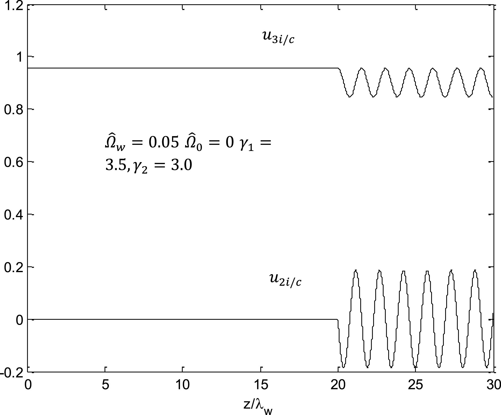
where, $\hat{{\it\Omega}}_{w}=(eB_{w})/(mc^{2}k_{w})$ is a function of the axial position ( $z$ ) and $\hat{{\it\Omega}}_{0}=(eB_{0})/(mc^{2}k_{w})$ is scaled GMF. As an example, we consider energy of the beams which corresponding to ${\it\gamma}_{1}=3.5$ , ${\it\gamma}_{2}=3.0$ and a wiggler field in which $\hat{{\it\Omega}}_{w}=0.05$ . We plot $u_{3i}$ and $u_{2i}$ versus axial position that is seen in figure 1. The electron trajectory exhibits small oscillations about the steady-state orbit. The value of $u_{2i}$ remain small $(u_{2i}\cong 0)$ over the entire course of the trajectory. Plot of $u_{3i}$ also exhibit a small oscillation about the value for the steady-state orbit; however mean value of it is less than its initial value.

Figure 1.

Plot of the single-particle trajectories versus axial distance for, $\hat{{\it\Omega}}_{w}=0.05$ , $\hat{{\it\Omega}}_{0}=0$ , ${\it\gamma}_{1}=3.5,{\it\gamma}_{2}=3.0$ .

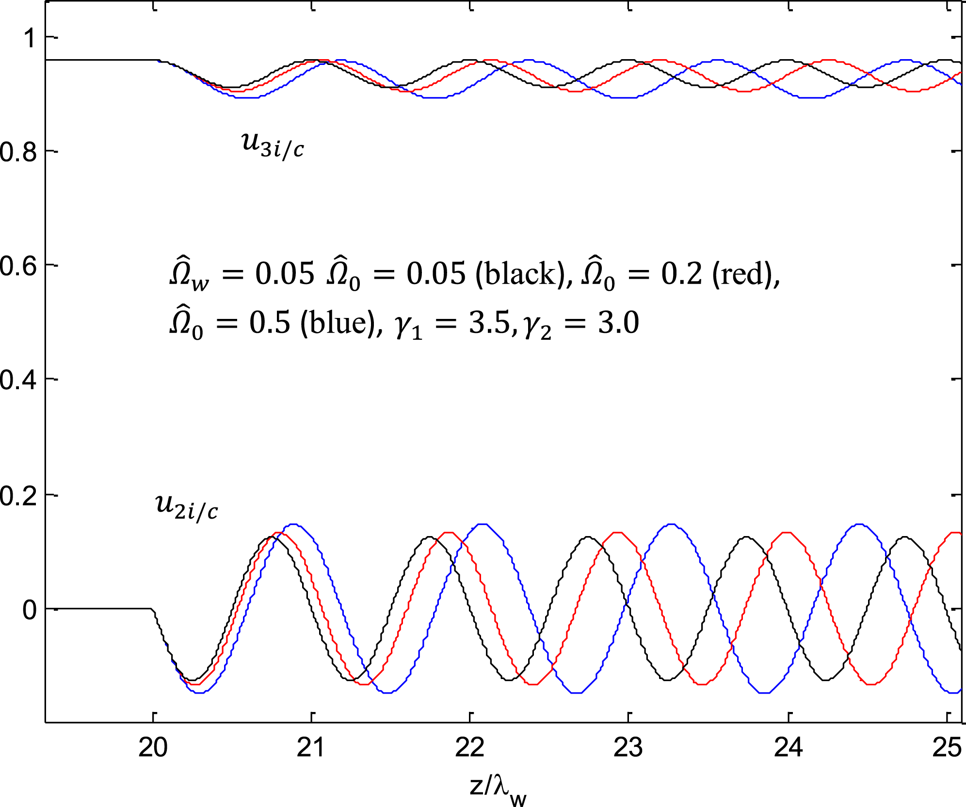
As magnitude of the $\hat{{\it\Omega}}_{0}$ (corresponding to an increase in GMF) increases from 0 to 0.62 the magnitude of the fluctuation relative to the steady-state bulk value $u_{2i}$ increases, this fact is shown in figure 2. Increases in $u_{2i}$ cause an increase in the interaction time of the particles with the wave and as a result it [increases in fluctuation of $u_{2i}$ ] causes to reach the shorter distance to saturation, which will be discussed in the next sections.

Figure 2.

Plot of the single-particle trajectories versus axial distance for $\hat{{\it\Omega}}_{w}=0.05$ , $\hat{{\it\Omega}}_{0}=0$ (black), $\hat{{\it\Omega}}_{0}=0.2$ (red), $\hat{{\it\Omega}}_{0}=0.5$ (blue), ${\it\gamma}_{1}=3.5,{\it\gamma}_{2}=3.0$ .

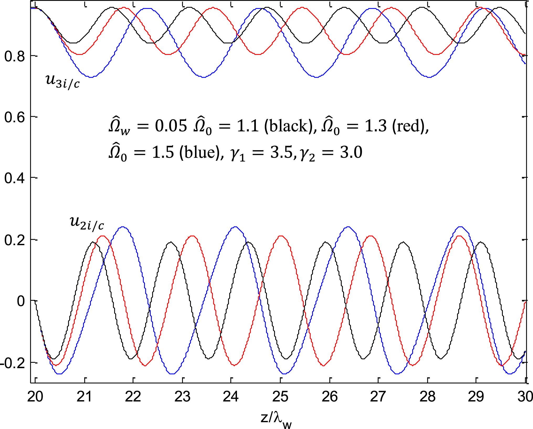
Parameters consistent with Group-II steady-state orbits are considered in figure 3. With an adiabatic rise in wiggler magnitude, we encounter an increase in the magnitude of $u_{2i}$ , however, small oscillations about mean values are found in constant wiggler amplitude region. In this regime, perturbation about the steady-state orbits is large. Although increasing the strange of the GMF along with the steady-state axial velocity, it causes to decrease the perturbations about the helical orbits, as is shown in figure 3.

Figure 3.

Plot of the single-particle trajectories versus axial distance for $\hat{{\it\Omega}}_{w}=0.05$ , $\hat{{\it\Omega}}_{0}=1.1$ (black), $\hat{{\it\Omega}}_{0}=1.3$ (red), $\hat{{\it\Omega}}_{0}=1.5$ (blue), ${\it\gamma}_{1}=3.5$ , ${\it\gamma}_{2}=3.0$ .

As the GMF strange is increased, perturbation about the steady-state orbits increases. In the special range of the GMF strange, (i.e.  $1.788\leqslant \hat{{\it\Omega}}_{0}$ ) for $\hat{{\it\Omega}}_{w}=0.05$ , ${\it\gamma}_{1}=3.5$ and ${\it\gamma}_{2}=3.0$ large fluctuations in the electron velocity occur. However, for $\hat{{\it\Omega}}_{0}\leqslant 1.788$ , transverse components of the electron velocity may become small which the radial excursions of the electron beam make it easy for the beams to propagate.

3. Particle-field equations

In order to derive the dynamical equations which govern the evolution of the radiation the scalar and vector potentials of radiation and space-charge wave are substituted into the Maxwell’s equations. The vector potential of the radiation field can be written as

and

where ${\it\delta}\hat{A}(z)$ and ${\it\delta}\widehat{\emptyset }(z)$ are the time-independent amplitudes of vector and scalar potentials. The phase of an electromagnetic wave of frequency ${\it\omega}$ and wavenumber $k_{+}$ is given by

and

is the phase of the space-charge wave with the same frequency but wavenumber $k$ . By substituting microscopic fields and source current in Maxwell’s equations and assuming slowly varying amplitudes and wavenumbers over a wavelength (slow time-scale approximation) one could obtain the field equations (Freund & Antonsen Reference Freund and Antonsen1996; Raghavi, De Ninno & Mehdian Reference Raghavi, De Ninno and Mehdian2008; Mahdizadeh & Aghamir Reference Mahdizadeh and Aghamir2012). The procedure is similar to (Freund & Antonsen Reference Freund and Antonsen1996; Raghavi et al. Reference Raghavi, De Ninno and Mehdian2008) and results are given in the following equations,

where, ${\it\Gamma}_{+}$ defines the growth rate (i.e. the logarithmic derivative) of the vector potential, ${\it\delta}a=(e{\it\delta}\hat{A}(\bar{z}))/mc^{2},{\it\delta}{\it\varphi}=(e{\it\delta}\widehat{\emptyset }(\bar{z}))/mc^{2}$ , ${\it\omega}_{bi}^{2}=(4{\rm\pi}n_{i}e^{2})/mc^{2}$ are the scaled amplitude of the vector potential, scaled amplitude of the space-charge potential and the plasma frequency denoted by the ambient beam density, respectively. Here, ${\it\psi}\equiv {\it\alpha}_{+}(\bar{z},\bar{t})+\bar{z}$ and ${\it\psi}_{sc}(\equiv {\it\alpha}(\bar{z},\bar{t}))$ are the ponderomotive and space-charge phases, respectively, which are given as In the above differential equations, we have changed the integration parameter from $\bar{t}$ to $\bar{z}$ , according to the relation $\text{d}/\text{d}\bar{t}={\it\beta}_{3}(\text{d}/\text{d}\bar{z})$ (which ${\it\beta}_{3i}=v_{3i}/c$ ). It is convenient to scale all quantities to $c$ (speed of light in vacuum) and $k_{w}$ , i.e.  $\bar{t}=tck_{w}$ , $\bar{z}=zk_{w}$ , $\bar{{\it\omega}}={\it\omega}/ck_{w}$ , $\bar{k}=k/k_{w}$ , $\bar{t}_{0}=t_{0}ck_{w}$ , $\bar{{\it\omega}}_{bi}={\it\omega}_{bi}/ck_{w}$ .

The averaging operator $\langle (\cdots \,)\rangle =(1/2{\rm\pi})\int _{-{\rm\pi}}^{{\rm\pi}}{\it\sigma}({\it\psi}_{0})\,\text{d}{\it\psi}_{0}(\cdots \,)$ is defined over an ensemble of beam electrons injected into the interaction region within one wave period. Here, ${\it\sigma}({\it\psi}_{0})$ refers to the initial beam distribution in phase. Since it is assumed that the beams are uniformly distributed, it is taken as ${\it\sigma}({\it\psi}_{0})=1$ where ${\it\psi}_{0}(=-\bar{{\it\omega}}\bar{t}_{0})$ is the initial phase, and $\bar{t}_{0}$ is scaled injection time. Derivation of dynamical equations (3.5a–d ) is presented in the appendix A.

Since we treat the case of a steady-state amplifier configuration, one may integrate z and write the Lorentz force equations as (Freund & Antonsen Reference Freund and Antonsen1996)

It has been assumed that the amplitudes and phases are slowly varying functions of position, i.e.  $|\partial {\it\delta}a/\partial z|\ll |k_{+}{\it\delta}a|$ , and this occurs only in a vicinity of the wave-particle resonance at ${\it\omega}\approx (k_{+}+k_{w})v_{3i}$ .

Equations (3.5) and (3.6) together with (3.7) give a set of $10N+4$ self-consistent first order nonlinear differential equations which describe the wave evolution in the two-stream FEL. Here $N$ refers to the total number of electrons, subjected to the initial conditions.

4. Numerical solutions

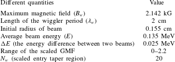
Using the fourth-order Runge–Kutta method, the set of coupled differential equations (3.5)–(3.7), has been solved numerically for a two-stream FEL working in amplifier mode. A wave ( ${\it\omega},k_{+}$ ) of arbitrary amplitude is injected into the system in concert with two relativistic, monoenergetic and noiseless electron beams. The typical parameters of the two-stream FEL system used in this work are the same with the numerical analyses which have been listed in table 1.

Table 1.

Two-stream FEL parameters under consideration.

The averages in the dynamical equations have been calculated by the Simpson’s rule in each of the variables with a total 17 semi-particles per wave period. The electrons are uniformly distributed in phase for $-{\rm\pi}\leqslant {\it\psi}_{0}\leqslant {\rm\pi}$ in order to model the case of a continual and un pre-bunched beam. The wiggler field is assumed to increase adiabatically to a constant level over twenty wiggler periods. Since the wiggler field increases adiabatically from zero at the entry plane, the growth rate of the vector potential is initially zero as well (i.e. $({\it\Gamma}_{+})_{0}=0$ ). The electromagnetic mode was chosen to correspond to the wave characterized by the highest linear growth rates. For a finite value of initial scalar potential and a uniform initial electron distribution the initial $\bar{k}$ value vanishes. The arbitrary initial values for the vector and scalar potentials are the same and they are of order $1.0\times 10^{-6}$ . Generally, the frequency of the amplified wave is determined by the intersection of the slow space-charge wave mode and the transverse electromagnetic mode.

Corresponding, the initial value of the axial velocity may be obtained by solving a cubic equation, which results from requiring the conservation of the total energy for the steady state orbits. Substituting ${\it\gamma}_{0i},{\it\omega}$ and $v_{0zi}$ into the transverse electromagnetic mode one can obtain the initial value of the $k_{+}$ .

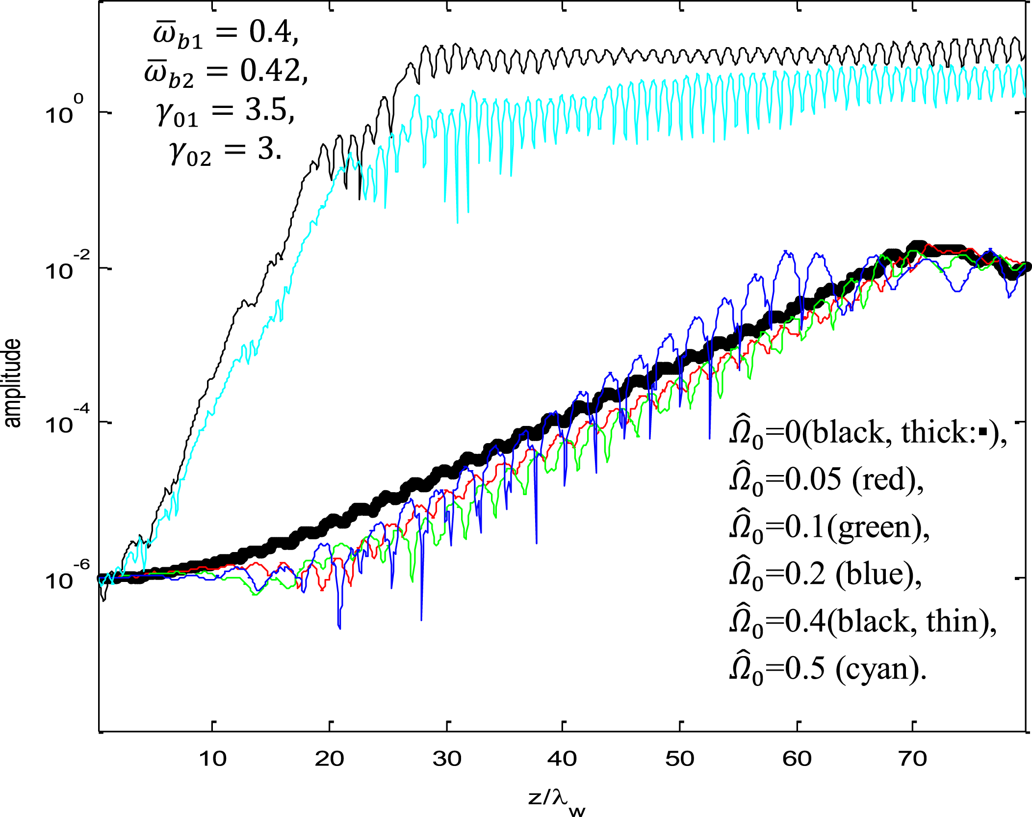
An example of the simulation results for the Group I orbit is shown in figure 4 in which the radiation field amplitude which is corresponding to the power is plotted as a function of axial position for the case in which $\hat{{\it\Omega}}_{w}=0.4$ , ${\it\gamma}_{1}=3.5$ , ${\it\gamma}_{2}=3.0$ , $\bar{{\it\omega}}_{b1}=0.4$ , $\bar{{\it\omega}}_{b2}=0.42$ , for some different value of the axial GMF such as: $\hat{{\it\Omega}}_{0}=0.05$ (red), $\hat{{\it\Omega}}_{0}=0.1$ (green) and $\hat{{\it\Omega}}_{0}=0.2$ (blue), $\hat{{\it\Omega}}_{0}=0.4$ (black, thin), $\hat{{\it\Omega}}_{0}=0.5$  (cyan) and without a GMF (black, thick: ▪). It is explicitly seen from the figure that, using GMF leads to an elevated increase in the amplitude and further decline in the distance to saturation. The input signal frequency depends on the axial GMF as well as the other initial two-stream FELs parameter. In the case of no GMF for $0<z/{\it\lambda}_{w}\leqslant 8.721$ , the amplitude which corresponds to the power remains almost at its initial value ( $\cong 10^{-6}$ ), such region corresponds to the small signal regime. Amplitude increases exponentially for $8.721\leqslant z/{\it\lambda}_{w}$ and continues the increase up to $z/{\it\lambda}_{w}\cong 70.37$ , which is the saturation point but the radiation amplitude does not increase. The region where amplitude increase exponentially i.e.  $8.721\leqslant z/{\it\lambda}_{w}<70.37$ is the nonlinear regime and $z/{\it\lambda}_{w}=70.37$ is the saturation point with scaled amplitude of ${\it\delta}a\cong 0.02005$ (for the case of $\hat{{\it\Omega}}_{0}=0$ ).

Figure 4.

Graphs of the amplitude of the radiation field versus axial coordinate for: $\hat{{\it\Omega}}_{0}=0$ (black, thick: ▪), $\hat{{\it\Omega}}_{0}=0.05$ (red), $\hat{{\it\Omega}}_{0}=0.1$ (green), $\hat{{\it\Omega}}_{0}=0.2$ (blue), $\hat{{\it\Omega}}_{0}=0.4$ (black, thin), $\hat{{\it\Omega}}_{0}=0.5$ (cyan).

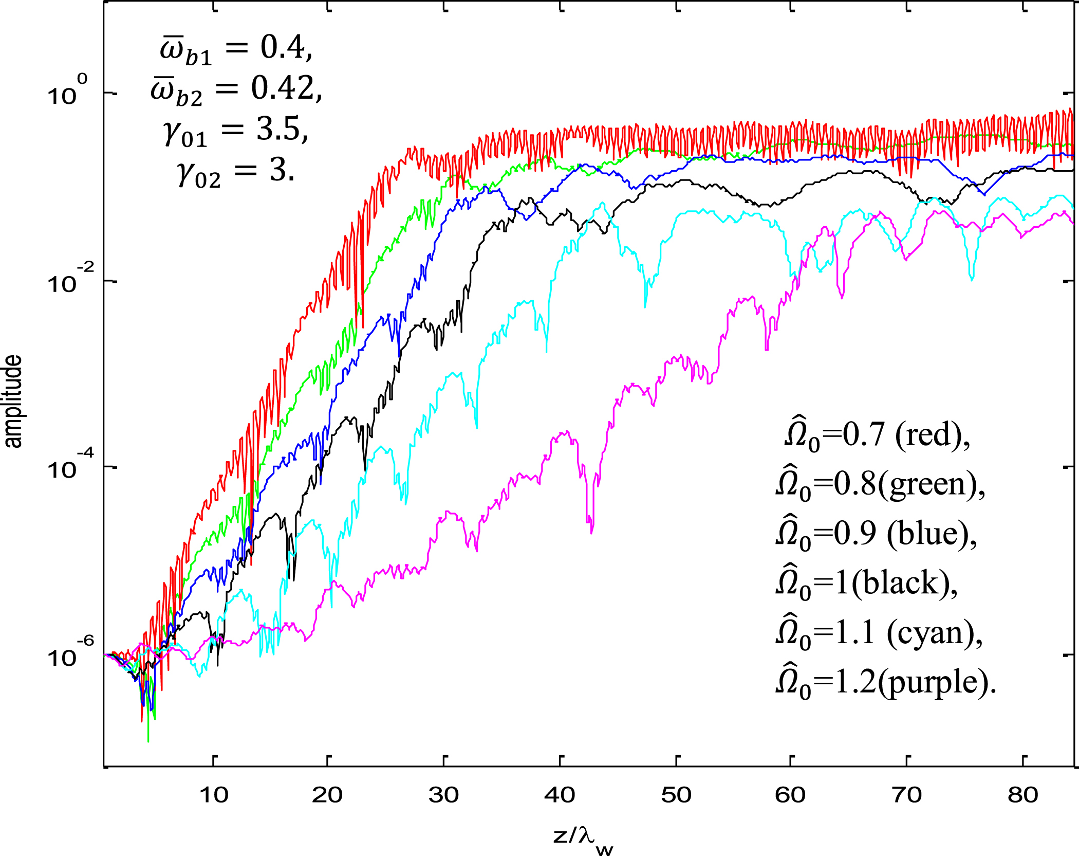
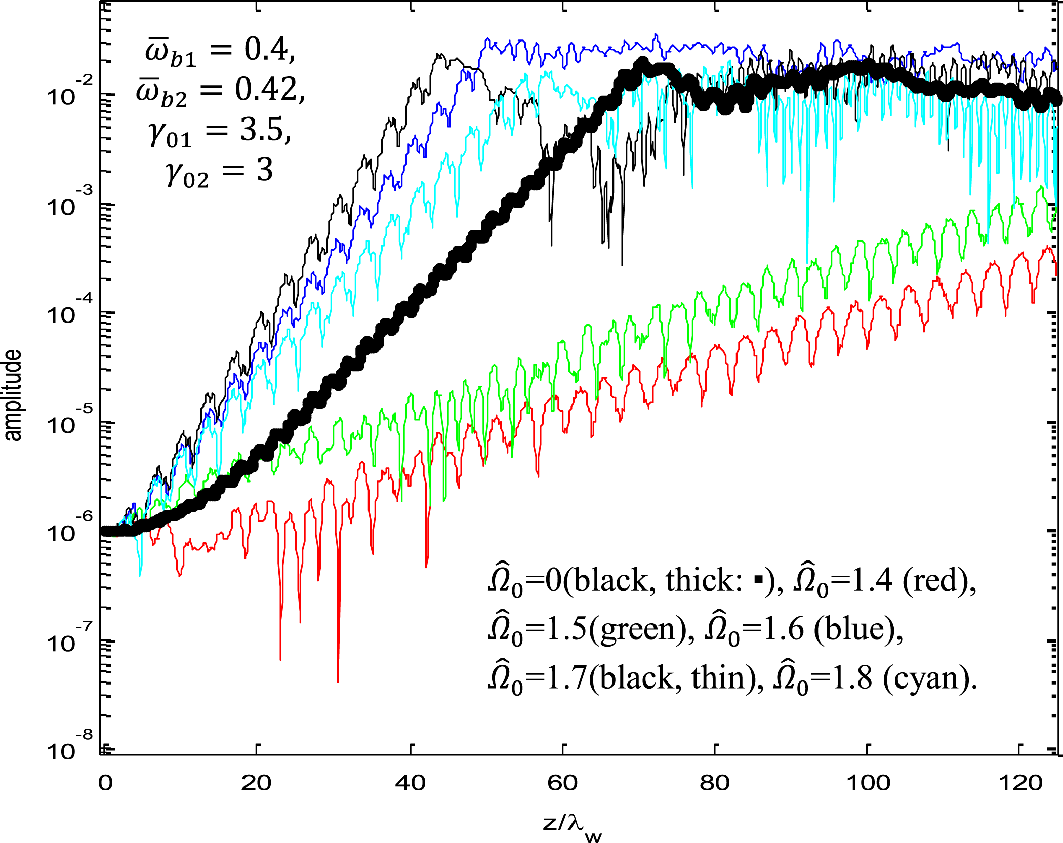
Different values of saturation point stemmed from different GMF strengths, as seen in figures 5 and 6. For instance, in the case of $\hat{{\it\Omega}}_{0}=0.5$ (cyan), the amplitude of the radiation begins to be amplified at $z/{\it\lambda}_{w}=2.51$ and the saturation point is at $z/{\it\lambda}_{w}=31.33$ with scaled amplitude of ${\it\delta}a\cong 2.29$ . This range of GMF corresponds to Group I single particle trajectories with $v_{0z1}/c=0.9715$ , $v_{0z2}/c=0.9434$ and in this range the resonant frequency as well as the efficiency are lower.

Figure 5.

Graphs of the amplitude of the radiation field versus axial coordinate for: $\hat{{\it\Omega}}_{0}=0.7$ (red), $\hat{{\it\Omega}}_{0}=0.8$ (green), $\hat{{\it\Omega}}_{0}=0.9$ (blue), $\hat{{\it\Omega}}_{0}=1$ (black), $\hat{{\it\Omega}}_{0}=1.1$ (cyan), $\hat{{\it\Omega}}_{0}=1.2$ (purple).

Figure 6.

Graphs of the amplitude of the radiation field versus axial coordinate for: $\hat{{\it\Omega}}_{0}=0$ (black,thick: ▪), $\hat{{\it\Omega}}_{0}=1.4$ (red), $\hat{{\it\Omega}}_{0}=1.5$ (green), $\hat{{\it\Omega}}_{0}=1.6$ (blue), $\hat{{\it\Omega}}_{0}=1.7$ (black, thin), $\hat{{\it\Omega}}_{0}=1.8$ (cyan).

Increases in the axial GMF lead to a longer distance to saturation above the value $\hat{{\it\Omega}}_{0}=0.5$ up to $\hat{{\it\Omega}}_{0}=1.4$ as shown in figures 4 and 5. It is worth mentioning that in order to compare the saturation distance, efficiency and single particle orbit in case there is GMF or not, all quantities for the two cases are the same i.e. total current, initial energy of the electrons and so on. To compare the effect of GMF on the distance to saturation and wave amplitude it is evident from figure 6 in which in the case of $\hat{{\it\Omega}}_{0}=1.7$ (black, thin), scaled distance to saturation is 43.67 (87.34 cm); however, in the case of no GMF it is 70.37 (140.74 cm). At the same time, scaled wave amplitude in the case of $\hat{{\it\Omega}}_{0}=1.7$ (black, thin) is 0.02399, however in the latter case is 0.02005 and scaled resonant frequency for two cases of $\hat{{\it\Omega}}_{0}=1.7$ (black, thin) and $\hat{{\it\Omega}}_{0}=0$ (black, thick) is the same and it is 5.837. The distance to saturation decrease to about 37.94 % because of the presence of the axial GMF; however, the decrease in the saturation length employing the ion-channel guide in FEL is about 30 % (Raghavi et al. 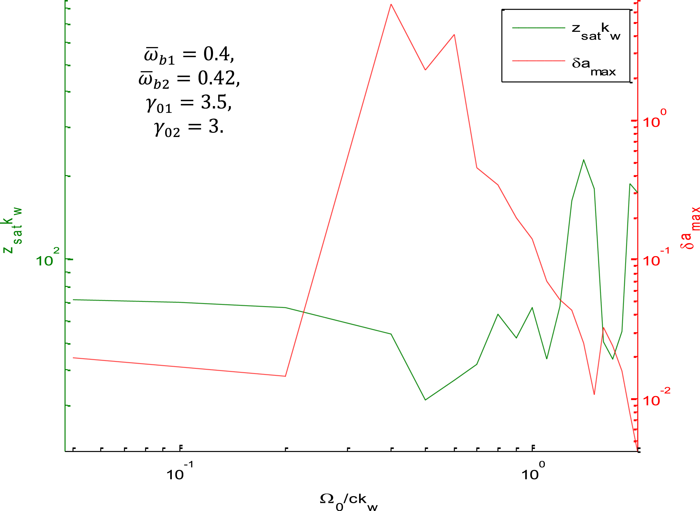Reference Raghavi, De Ninno and Mehdian2008). But, the wave amplitude does not have a considerable increase within both output enhancement (i.e. the ion-channel and axial GMF). The beating of the wiggler and the electromagnetic wave result in the ponderomotive potential and when the bunched electrons trapped in that’s potential saturation occurs, upsurges in the GMF cause (1) to increase the fluctuation levels in the electron velocities about the steady-state trajectories, (2) decrease axial component of velocities, alternatively, increase quiver velocity (3) decline divergence of the electron beam and these effects will compete with the increases in the efficiency and power. A summary of the distance to saturation and maximum amplitude of radiation are shown in figure 7 as functions of scaled GMF.

Figure 7.

Graphs of the distance to saturation (dashed line) and the maximum amplitude (dotted line) versus scaled GMF strength.

It is evident from figure 7 that shorter distance to saturation occur for $\hat{{\it\Omega}}_{0}=0.5$ . Initially distance to saturation decreases for values $\hat{{\it\Omega}}_{0}<0.5$ then increases (for the range of $0.5<\hat{{\it\Omega}}_{0}<1.4$ ), after that decreases (for the range of $1.4<\hat{{\it\Omega}}_{0}<1.7$ ) and finally increases. Using the GMF cause to increases maximum amplitude of radiation. The larger amplitude occurs for the scaled GMF strange of $\hat{{\it\Omega}}_{0}=0.4$ . More increases in GMF strength decrease the maximum amplitude of radiation as shown in figure 7.

Figure 8.

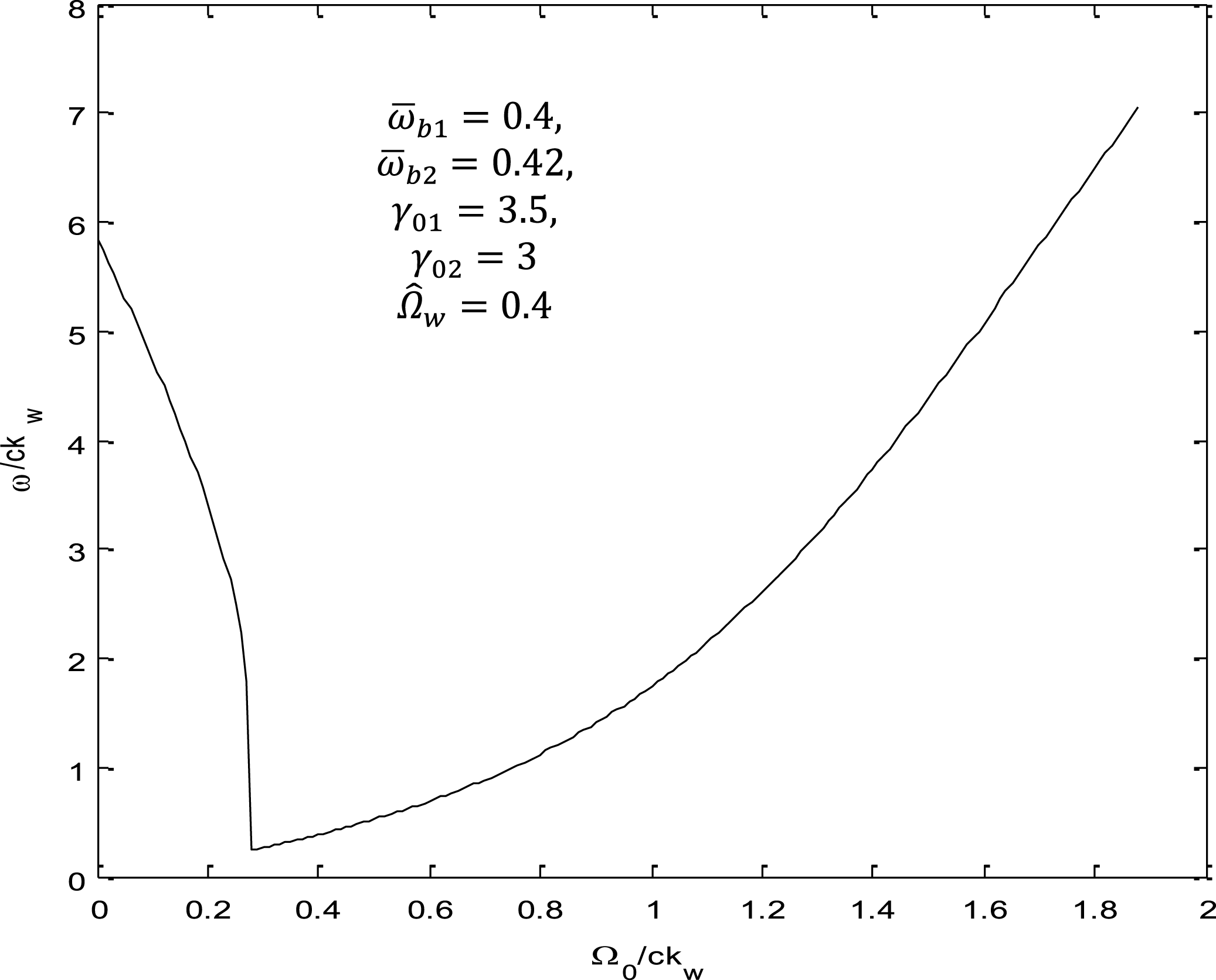
Graphs of the resonant frequency versus axial GMF strange for $\hat{{\it\Omega}}_{w}=0.4$ , $\bar{{\it\omega}}_{b1}=0.4,\bar{{\it\omega}}_{b2}=0.42,{\it\gamma}_{01}=3.5,{\it\gamma}_{02}=3$ .

The resonant frequency versus axial GMF strange for a typical value of wiggler strange ( $\hat{{\it\Omega}}_{w}=0.4$ ) was shown in figure 8. First resonant frequency decreases and then for the range of $\hat{{\it\Omega}}_{0}>0.287$ it increases. By adjusting the axial GMF strange, tuning a given wiggler configuration at different output wavelength is applicable. For a benchmark in our study, when we consider all quantities of each beam equal to zero results of Freund & Antonsen (Reference Freund and Antonsen1996), Raghavi et al. (Reference Raghavi, De Ninno and Mehdian2008) are recovered.

Figure 9.

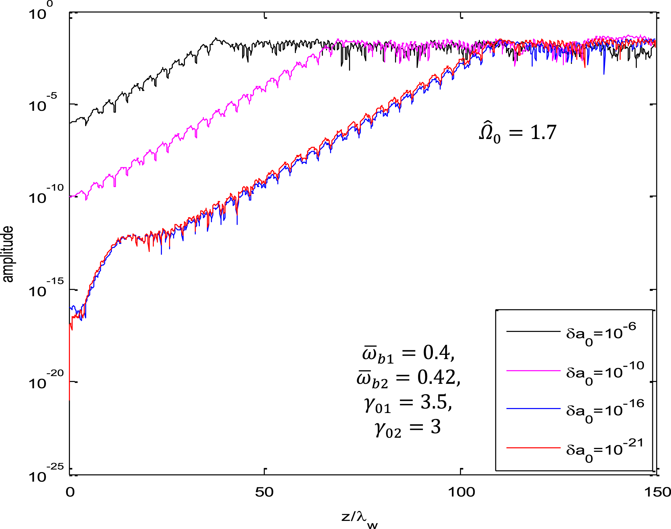
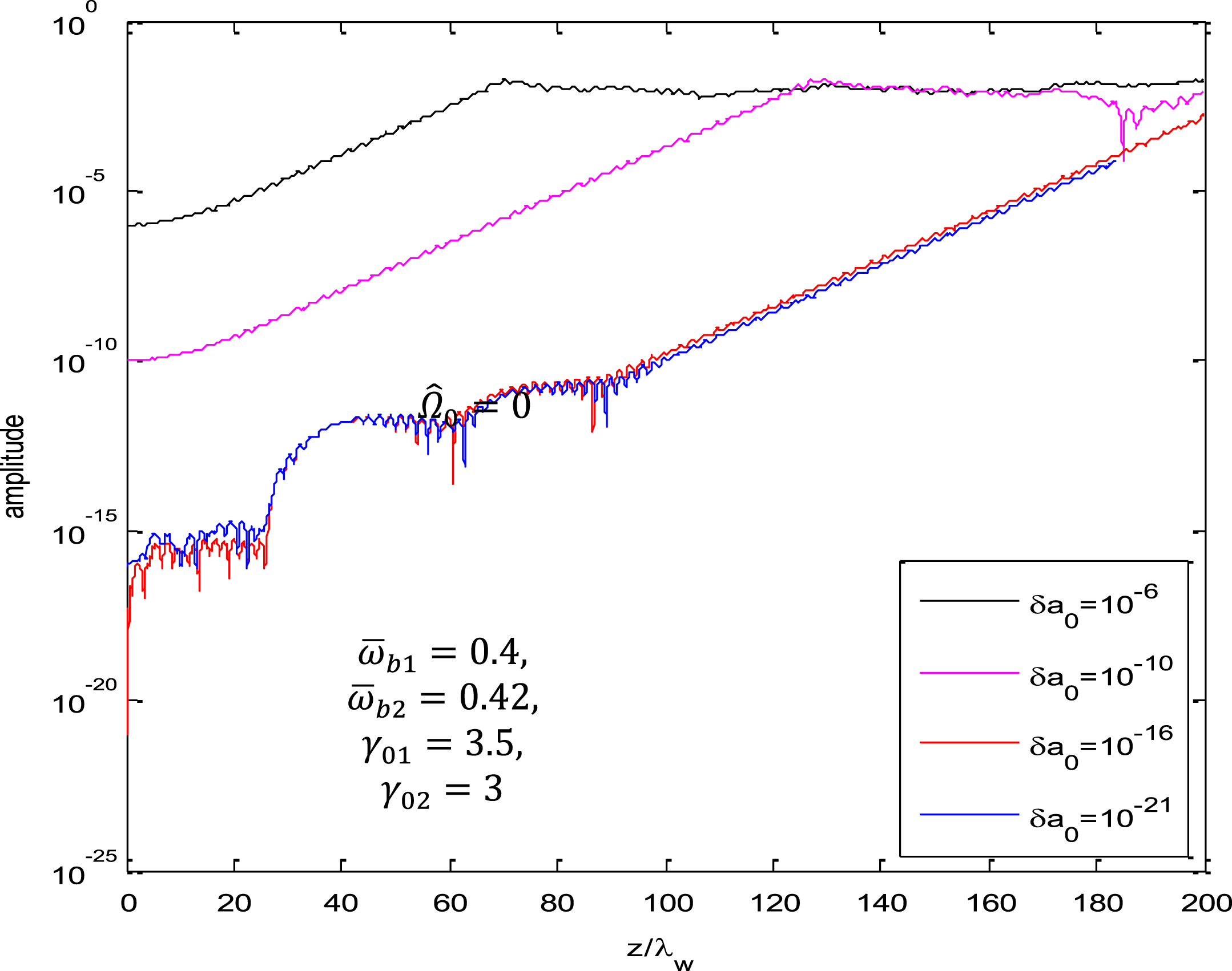
Graphs of the amplitude of the radiation field versus axial coordinate for different value of the seed intensity.

Figure 10.

Graphs of the amplitude of the radiation field versus axial coordinate for different value of the seed intensity.

Maximum wave amplitude of the output radiation does not depends on the initial amplitude of the seed. However, for the seeds with the least initial amplitude, ratio of the final electromagnetic (EM) wave amplitude to the initial amplitude have maximum value, as shown in figures 9 and 10. It is evident from the figures that the seeds with high intensity decreases the distance to saturation because the seeds with high intensity hastens bunching process of the electron and result particle trapping in the ponderomotive potential. The efficiency can be defined as the ratio of the output radiation field energy-flux increase to the initial beams-energy-flux and it is given by

where the ${\it\eta}$ shows net energy transfers to the wave and ${\it\delta}a_{sat}$ is the radiation field amplitude at saturation.

Figure 11.

Graphs of the efficiency versus scaled longitudinal distance for: $\hat{{\it\Omega}}_{0}=0$ (blue), $\hat{{\it\Omega}}_{0}=1.7$ (red).

The axial position dependence of the linear efficiency is illustrated in figure 11 for two cases with and without considering the GMF. It is clear from the figure that efficiency increases while we consider the GMF. In the case of no GMF it is about mean value 1.65 %. However, when we consider GMF it is about 2.61 %. in this case, the evolution of radiation fields become more regular as well.

Figure 12.

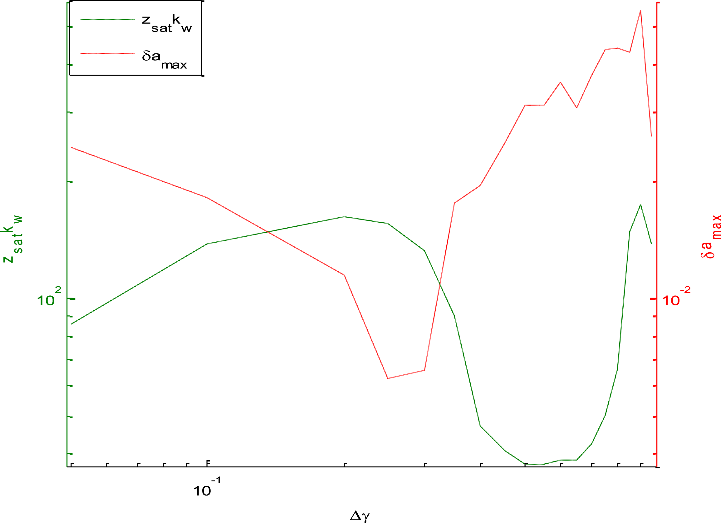
Graphs of the maximum amplitude (red) and the distance to the saturation (azure) versus scaled the difference of initial two beams energy.

Maximum amplitude and the distance to saturation as a function of scaled the difference of initial two beams energy are plotted in figure 12. It is evident from the figure that for the value of ${\rm\Delta}{\it\gamma}=0.9$ the amplitude of the radiation has maximum value; however, for the range of $0.45\leqslant {\rm\Delta}{\it\gamma}\leqslant 0.65$ distance to saturation have minimum value. On the other hand, for the range out of $0.45\leqslant {\rm\Delta}{\it\gamma}\leqslant 0.65$ the distance to saturation increases. As was seen in figure 6 employing an axial GMF does not affect strongly the amplitude of the radiation output. Thus, the difference value of the initial energy of two beams (which corresponds to relativistic factor) that we chose for our simulation is reasonable.