Introduction
Classical molecular dynamics (MD) simulation is an effective tool to access the atomic structure of glass, which usually remains invisible from traditional experimental techniques.[Reference Huang, Kurasch, Alden, Shekhawat, Alemi, McEuen, Sethna, Kaiser and Muller1–Reference Du, Massobrio, Du, Bernasconi and Salmon3] In turn, better understanding the atomic structure of glasses is key to decipher their genome, that is, to understand how their composition and structure control their engineering properties.[Reference Bauchy4] However, the accuracy of glass modeling based on MD simulations largely depends on the reliability of the underlying empirical forcefield, i.e., two-body (and sometimes three-body or more) interatomic potential.[Reference Du, Massobrio, Du, Bernasconi and Salmon3,Reference Yu, Wang, Wang, Sant and Bauchy5] Although ab initio molecular dynamics (AIMD) can, in theory, overcome these limitations, the high-computational cost of this technique renders challenging glass simulations—which typically require large systems for statistical averaging and long timescales to slowly quench a melt down to the glassy state.[Reference Du, Massobrio, Du, Bernasconi and Salmon3,Reference Li, Song, Yang, Krishnan, Wang, Smedskjaer, Mauro, Sant, Balonis and Bauchy6,Reference Ganster, Benoit, Delaye and Kob7] The development of new, improved empirical forcefields presently represents a bottleneck in glass modeling.[Reference Behler8–Reference Bartók, Kermode, Bernstein and Csányi10]
Empirical forcefields are typically based on functionals that depend on several parameters (e.g., partial atomic charges, etc.), which need to be properly optimized in order to minimize a given cost function.[Reference Sundararaman, Huang, Ispas and Kob11,Reference Wang, Anoop Krishnan, Wang, Smedskjaer, Mauro and Bauchy12] One option is to define the cost function in terms of the difference between the structure or properties of the simulated system and available experimental data. However, such an optimization method may not yield a realistic forcefield in the case of glassy materials, since simulated and experimental glasses are prepared with significantly different cooling rates and, hence, their direct comparison may not be meaningful.[Reference Li, Song, Yang, Krishnan, Wang, Smedskjaer, Mauro, Sant, Balonis and Bauchy6,Reference Lane13] Although this problem can be partially overcome by conducting the optimization based on crystals rather than glasses, crystal-based potentials do not always properly describe the structure and properties of disordered, out-of-equilibrium glasses.[Reference Wang, Anoop Krishnan, Wang, Smedskjaer, Mauro and Bauchy12] Alternatively, empirical forcefield can be parameterized based on AIMD simulations.[Reference Carré, Ispas, Horbach and Kob9,Reference van Beest, Kramer and van Santen14,Reference Carré, Horbach, Ispas and Kob15] However, directly optimizing the forcefield in order to match with the interatomic forces or energy derived from AIMD sometimes results in unrealistic structures for the simulated glasses.[Reference Carré, Ispas, Horbach and Kob9,Reference Sundararaman, Huang, Ispas and Kob11,Reference Ercolessi and Adams16] Recently, Kob and Huang et al. proposed a new optimization scheme, wherein the optimization cost function is defined based on the difference between the structure of a simulated liquid and that obtained by AIMD simulations under similar conditions.[Reference Carré, Ispas, Horbach and Kob9,Reference Sundararaman, Huang, Ispas and Kob11,Reference Carré, Horbach, Ispas and Kob15] However, such cost functions are very “rough,” that is, they exhibit a large number of local minima (i.e., several sets of parameters yield similar, competitive results). This is a challenge as conventional gradient-based optimization methods [e.g., steepest descent or conjugate gradient (CG)] are highly inefficient to explore rough functions and are likely to yield a local minimum rather than the global one.[Reference Shewchuk17] Due to this issue, conventional optimization methods are often biased, that is, their outcomes strongly depend on the starting point.
As an alternative route to conventional “intuition-based” forcefield parameterization, artificial intelligence and machine learning (ML) techniques have potential to offer some efficient, non-biased optimization schemes.[Reference Gubernatis and Lookman18,Reference Ramprasad, Batra, Pilania, Mannodi-Kanakkithodi and Kim19] To this end, several ML-based forcefields have been proposed.[Reference Behler8,Reference Huan, Batra, Chapman, Krishnan, Chen and Ramprasad20,Reference Li, Li, Pickard, Narayanan, Sen, Chan, Sankaranarayanan, Brooks and Roux21] However, although such forcefields can approach the accuracy of AIMD at a fraction of computing cost, their parameterization remains tedious and the complex form of the resulting forcefields render challenging their physical interpretation and their implementation.[Reference Bartók, Kermode, Bernstein and Csányi10,Reference Huan, Batra, Chapman, Krishnan, Chen and Ramprasad20–Reference Hellström, Behler, Andreoni and Yip22] For these reasons, ML-based forcefields have thus far mostly been limited to simple systems (e.g., comprising only one element at a time[Reference Bartók, Kermode, Bernstein and Csányi10,Reference Deringer and Csányi23] ), which does not yet offer a realistic path toward the simulation of complex multi-component glasses.
Here, we present a new less accurate, but more pragmatic approach to efficiently parameterize forcefields based on ML-based optimization. Our method is based on a predefined empirical potential form, wherein the parameters are optimized versus AIMD simulations by Gaussian process regression (GPR) and Bayesian optimization (BO). We illustrate our new method by taking the example of glassy silica (g-SiO2), an archetypal model for complex silicate glasses. Our method yields a new interatomic forcefield for g-SiO2 that offers an unprecedented agreement with ab initio simulations. We demonstrate that, compared with traditional optimization methods, our ML-based optimization scheme is more efficient and non-biased. Overall, this work provides a realistic pathway toward the accurate, yet computationally efficient simulation of non-equilibrium disordered materials.
This paper is organized as follows. First, “Methods” section describes the technical details of the simulations and parameterization strategy. The application of our method to glassy silica is then presented in the “Results” section. We then discuss the advantage of our approach over conventional optimization methods in the “Discussion” section. Finally, some conclusions are given in the “Conclusions” section.
Methods
Reference ab initio simulations
A “reference” structure of a liquid silica system is first prepared by Car–Parrinello molecular dynamics (CPMD).[Reference Car and Parrinello24] The simulated system comprises 38 SiO2 units (114 atoms) in a periodic cubic simulation box of length 11.982 Å—in accordance with the experimental density of 2.2 g/cm3.[Reference Bansal and Doremus25] The electronic structure is described with the framework of density functional theory and the choice of pseudopotentials for silicon and oxygen, exchange and correlation functions, and the plane-wave cutoff (70 Ry) are based on previous CPMD simulations of glassy silica.[Reference Carré, Ispas, Horbach and Kob9,Reference Carré, Horbach, Ispas and Kob15] A timestep of 0.0725 fs and a fictitious electronic mass of 600 atomic units are used. An initial liquid configuration is first prepared by conducting a classical MD run at 3600 K using the well-established van Beest–Kramer–van Santen (BKS) potential (see section “Classical molecular dynamics simulations”).[Reference van Beest, Kramer and van Santen14] The obtained configuration is then relaxed via CPMD at 3600 K for 3.5 ps at constant volume. Such duration is long enough considering the small relaxation time of the system at such elevated temperature. A subsequent dynamics of 16 ps is then used for statistical averaging and to compute the Si–Si, Si–O, and O–O partial pair distribution functions (PDFs) of the simulated liquid system. More details can be found in Refs. Reference Carré, Ispas, Horbach and Kob9 and Reference Carré, Horbach, Ispas and Kob15
Classical molecular dynamics simulations
A new empirical forcefield for g-SiO2 is then parameterized by conducting some classical MD simulations. The simulated system comprises 1000 SiO2 units (3000 atoms) in a periodic cubic simulation box of length 35.661 Å, which corresponds to an experimental density of 2.2 g/cm3.[Reference Bansal and Doremus25] An initial configuration is first prepared by relaxing the system for 10 ps at 3600 K in the NVT ensemble. The partial PDFs of the simulated systems are then computed based on a subsequent NVT dynamics of 10 ps. A timestep of 1 fs is used for all simulations.
The interatomic potential energy between each pair of atom i, j is here described by adopting the Buckingham form[Reference Carré, Ispas, Horbach and Kob9,Reference van Beest, Kramer and van Santen14] :
 $$U_{ij} = \displaystyle{{q_iq_j} \over {4\pi \varepsilon _0r_{ij}}} + A_{ij}\exp \left( {-\displaystyle{{r_{ij}} \over {\rho_{ij}}}} \right)-\displaystyle{{C_{ij}} \over {r_{ij}^6}} + \displaystyle{{D_{ij}} \over {r_{ij}^{24}}} $$
where r ij is the distance between each pair of atoms, q i is the partial charge of each atom (q O for oxygen, q Si for silicon, so that q O = −q Si/2), ε 0 is the dielectric constant, and the parameters A ij, ρ ij, C ij, and D ij describe the short-range interactions. A cutoff of 8 Å is used for the short-range interactions. The long-range Coulombic interactions are evaluated by a damped shifted force model[Reference Fennell and Gezelter26] with a damping parameter of 0.25 and a cutoff of 8 Å. The last term serves as to add a strong repulsion at short distance to prevent the “Buckingham catastrophe”.[Reference Carré, Ispas, Horbach and Kob9] Since this term only aims to prevent any atomic overlap, the D ij parameters are not included in the present optimization and their value is fixed based on Ref. Reference Carré, Ispas, Horbach and Kob9 (viz., D ij = 113, 29, and 3,423,200 eV Å24 for O–O, Si–O, and Si–Si interactions, respectively). Note that this Buckingham formulation is chosen as it typically provides a good description of ionocovalent systems and has been shown to offer an improved description of g-SiO2 as compared to alternative forms (e.g., Morse formulation).[Reference Sundararaman, Huang, Ispas and Kob11]
Optimization cost function
In total, the parameterization of this potential [Eq. (1)] requires the optimization of ten independent parameters, namely, the partial charge q Si and the short-range parameters {A ij, ρ ij, C ij} for each of the three atomic pairs (Si–O, O–O, and Si–Si). This set of parameters is denoted Ξ hereafter. Following Kob and Huang et al., we define the optimization cost function R x as follows[Reference Carré, Ispas, Horbach and Kob9,Reference Sundararaman, Huang, Ispas and Kob11,Reference Carré, Horbach, Ispas and Kob15] :
 $$R_{\rm x} = \sqrt {\displaystyle{{\chi _{{\rm SiO}}^2 + \chi _{{\rm OO}}^2 + \chi _{{\rm SiSi}}^2} \over 3}} $$
where the  $\chi _{a\beta} ^2 $ terms capture the level of agreement between the partial PDFs obtained by classical MD and AIMD[Reference Wright27]:
 $$\chi _{a\beta} ^2 = \displaystyle{{\sum\nolimits_r {{[g_{a\beta} ^{{\rm AIMD}} (r)-g_{a\beta} ^{{\rm MD}} (r)]}^2}} \over {\sum\nolimits_r {{[g_{a\beta} ^{{\rm AIMD}} (r)]}^2}}} $$
where  $g_{a\beta} ^{{\rm AIMD}} (r)$ and
 $g_{a\beta} ^{{\rm MD}} (r)$ are the partial PDFs for each pair of atoms α–β.
Although additional properties (e.g., energy, stiffness, etc.) could be included, we herein restrict the cost function to the difference between AIMD and MD partial PDFs. This choice is motivated by the following facts. (i) Although other structural descriptors could be used to describe the structure of the simulated glasses, the PDF offers a convenient description of the short-range environment around each atom[Reference Carré, Ispas, Horbach and Kob9,Reference Carré, Horbach, Ispas and Kob15] and, hence, capture some important features of the atomic structure. (ii) We purposely exclude from the training set any properties of glassy SiO2 (e.g., experimental density or stiffness) as such properties are not uniquely defined and depend on the cooling rate. (iii) Including some additional properties (i.e., besides the PDFs) in the cost function would raise the question of which weight to attribute to each property—which would render the parameterization of the forcefield biased to this arbitrary choice.
Forcefield optimization by machine learning
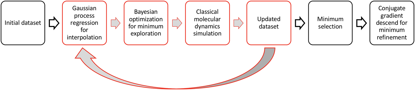
We now describe the ML-based optimization scheme used herein to parameterize the forcefield. An overview of the parameterization process is presented in Fig. 1. First, we create an initial dataset comprising some “known points,” that is, the values of the cost function R x for select sets of parameters Ξ. GPR[Reference Frazier and Wang28,Reference Rasmussen and Williams29] is then used to interpolate the known points and assess the interpolation uncertainty over the entire parameter space. The BO based on the expected improvement method[Reference Frazier and Wang28] is then used to predict an optimal set of parameters Ξ that offers the best “exploration versus exploitation trade-off,” that is, the best balance between (i) exploring the parameter space and reducing the model uncertainty and (ii) finding the global minimum of the cost function. The cost function R x{Ξ} associated with the set of parameters predicted by BO is subsequently calculated by conducting a classical MD simulation and comparing the structure of the simulated liquid with that of the reference AIMD configuration (see section “Optimization cost function”). This new datapoint R x{Ξ} is then added to the dataset. The new dataset is then used to refine the GPR-based interpolation and predict a new optimal set of parameters by BO. This cycle is iteratively repeated until a satisfactory minimum in the cost function is obtained (i.e., after about 600 iterations in this work). Finally, the global minimum predicted by BO is further refined by conducting a CG optimization.[Reference Shewchuk17]
Flowchart diagram summarizing our parameterization strategy.
Results
New interatomic forcefield for glassy silica
We conduct the optimization of the forcefield while keeping the Si–Si interaction energy term as being zero (i.e., A SiSi = C SiSi = 0 and ρ SiSi = 1 Å). This choice is motivated by the fact that the original BKS potential does not comprise any Si–Si interaction energy terms, which suggests that the addition of these terms may not be necessary. In turn, decreasing the number of variable parameters allows us to increase the efficiency of the optimization. In addition, decreasing the complexity of the forcefield limits the risk of overfitting, which, in turn, is likely to increase the transferability of the new forcefield to new systems that are not considered during its training. The effect of the complexity of the forcefield (and of Si–Si terms) is further discussed in Ref. Reference Liu, Fu, Li, Sabri and Bauchy30.
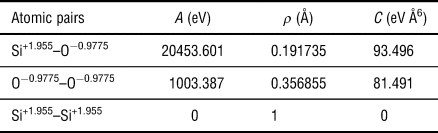
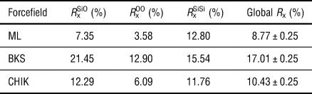
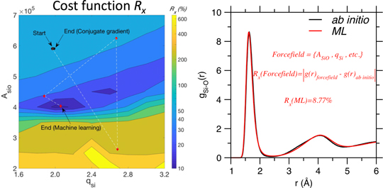
The forcefield parameters obtained after the BO and CG optimization steps are listed in Table I. The performance of our forcefield (as quantified in terms of the final cost function R x) is compared with that of select alternative potentials in Table II. We find that our new ML forcefield yields an R x of 8.77%. This constitutes a significant improvement with respect to the well-established BKS potential (for which R x is about 17%).[Reference van Beest, Kramer and van Santen14,Reference Wang, Yu, Lee and Bauchy31] Our new potential is also found to be slightly better than the CHIK potential parameterized by Kob et al..[Reference Carré, Horbach, Ispas and Kob15] This is not surprising as the CHIK potential was obtained based on the optimization of a slightly different cost function.[Reference Carré, Horbach, Ispas and Kob15] However, it is worth noting that our new potential exhibits a lower complexity than the CHIK parameterization (which comprises three extra parameters for the Si–Si interactions).
Parameters of our new interatomic potential “ML” [see Eq. (1)].

The partial charges are indicated as subscripts for each pair of atoms.
Comparison of our new “ML” forcefield with select alternative classical potentials, namely, “BKS”[Reference van Beest, Kramer and van Santen14] and “CHIK.”[Reference Carré, Horbach, Ispas and Kob15]

In detail, we find that the parameters of our ML forcefield are significantly different from those of the original BKS potential—which illustrates the roughness of the cost function. Interestingly, we find that our ML potential relies on a partial charge for Si atoms that is significantly smaller than that of the BKS potential (+1.955 versus +2.4 for BKS). In turn, this value is close to that of the CHIK (+1.91[Reference Carré, Horbach, Ispas and Kob15]) and Wang–Bauchy potential (+1.89[Reference Wang, Anoop Krishnan, Wang, Smedskjaer, Mauro and Bauchy12]). This suggests that “soft potentials” (i.e., which relies on lower partial charges) appear to consistently perform better than the stiffer ones, e.g., BKS. The cost function R x associated with each interatomic pair [see Eq. (3)] is also provided in Table II. Overall, we note that our ML potential consistently offers an improved description of the interatomic structural order for each pair of atoms.
Partial pair distribution functions
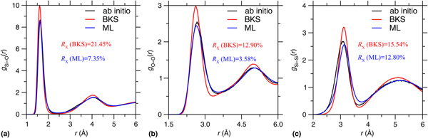
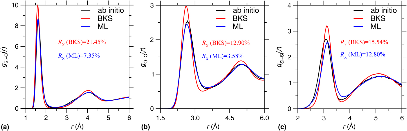
We now further analyze the structure of the simulated SiO2 liquid (i.e., at 3600 K). Figure 2 shows the partial PDFs predicted by our new ML forcefield. The data are compared with the reference ab initio partial PDFs used for the training of the potential[Reference Carré, Horbach, Ispas and Kob15] as well as those predicted by the BKS potential.[Reference van Beest, Kramer and van Santen14] Overall, we find that our ML forcefield offers an excellent agreement with AIMD simulations—although this is not surprising as our forcefield is specifically trained to match these data. Nevertheless, these results show that the Buckingham formulation adopted herein is appropriate for the SiO2 system and further supports the ability of our optimization method to offer a robust parameterization. We note that the average Si–Si distance predicted by our potential is slightly shifted with respect to that obtained in AIMD simulations [see Fig. 2(c)]. This may arise from a general limitation of the Buckingham formulation. Nevertheless, our ML forcefield offers a significant improvement with respect to the BKS potential, especially in the case of the Si–O and O–O partial PDFs (see also Table II). We note that our ML forcefield systematically predicts some PDF peaks that are broader than those predicted by BKS, which suggests that our forcefield yields a slightly more disordered structure. This may be linked with the fact that our potential relies on lower partial charge values (i.e., softer Coulombic interactions).
(a) Si–O, (b) O–O, and (c) Si–Si partial PDFs in liquid silica (at T = 3600 K) predicted by our new “ML” forcefield and compared with the ab initio reference.[Reference Carré, Horbach, Ispas and Kob15] The partial PDFs predicted by the BKS potential are added for comparison.[Reference van Beest, Kramer and van Santen14]
Partial bond angle distributions
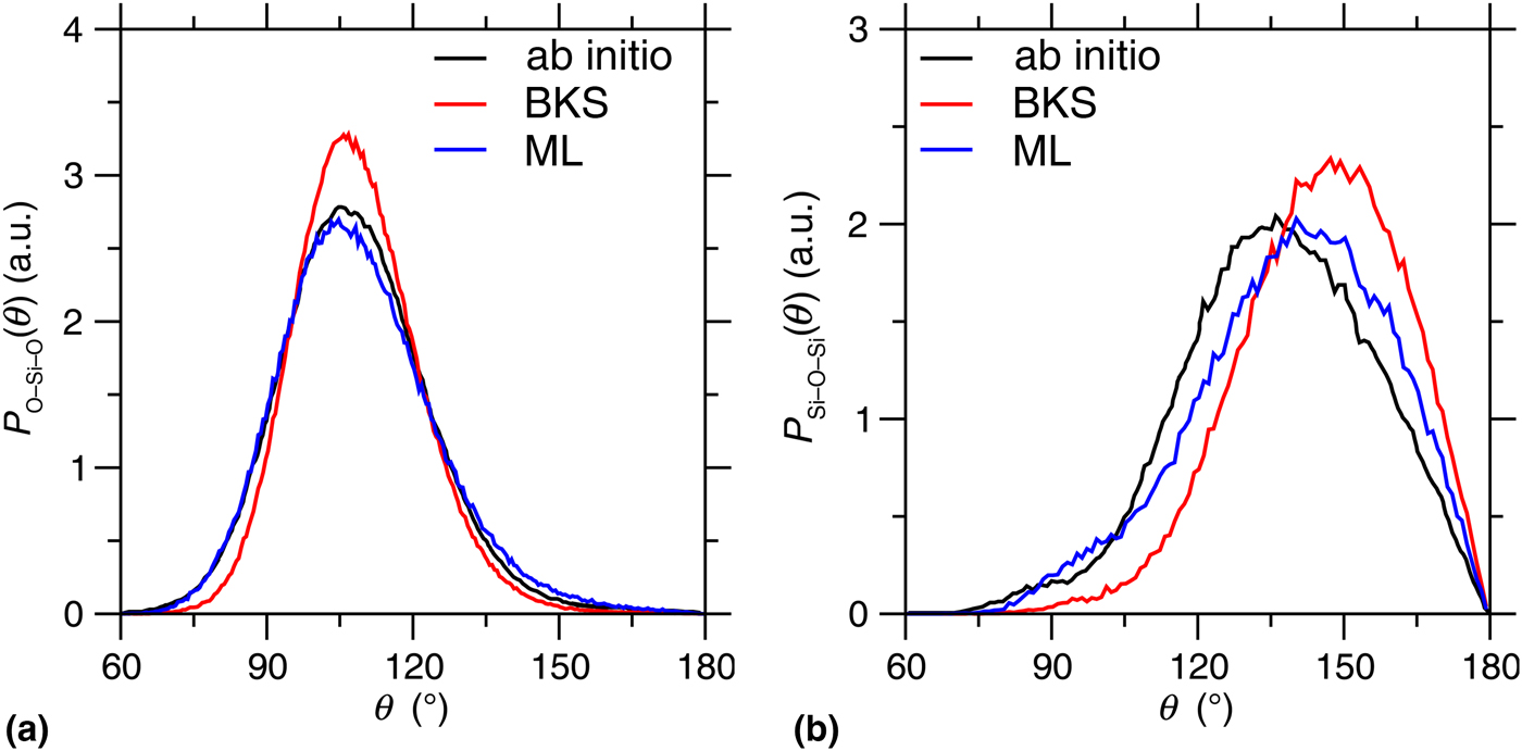
We now focus on the angular environment around each atom. To this end, Fig. 3 shows the O–Si–O and Si–O–Si partial bond angle distributions (PBADs) predicted by our ML forcefield for the liquid silica system (at T = 3600 K). The data are compared with those obtained by ab initio simulations[Reference Carré, Horbach, Ispas and Kob15] and predicted by the BKS potential.[Reference van Beest, Kramer and van Santen14] Overall, we observe that the PBADs predicted by our ML forcefield are in very good agreement with those obtained by ab initio simulations—with a significant improvement with respect to the BKS potential. This is significant as the PBADs are not explicitly included in the cost function used herein and such three-body correlations are not fully encoded in two-body correlations (i.e., as captured by the partial PDFs). As such, these results offer a strong a posteriori validation of the performance of our new ML forcefield.
(a) O–Si–O and (b) Si–O–Si PBADs in liquid silica (at T = 3600 K) predicted by our new “ML” forcefield and compared with the ab initio reference.[Reference Carré, Horbach, Ispas and Kob15] The PBADs predicted by the BKS potential are added for comparison.[Reference van Beest, Kramer and van Santen14]
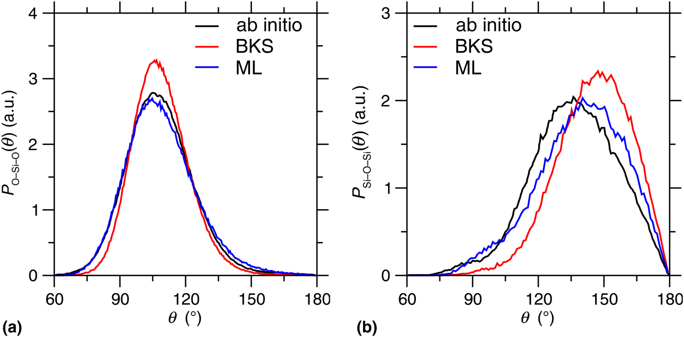
As expected, our forcefield yields a tetrahedral environment for Si atoms (with an average O–Si–O angle of about 109°). However, we note that the O–Si–O PBAD predicted by our ML forcefield is broader than that obtained with BKS, which suggests that our potential yields a slightly more disordered angular environment around Si atoms. Again, this may be linked with the fact that our potential relies on lower fictive charges than BKS (see section “Partial pair distribution functions”). In contrast, we observe that our forcefield slightly overestimates the value of Si–O–Si angle with respect to AIMD simulations. This is likely linked with the fact that our potential overestimates the Si–Si average distance (see section “Partial pair distribution functions”), which appears to be a general limitation of the two-body Buckingham formulation. Nevertheless, the Si–O–Si PBAD yielded by our forcefield is significantly improved with that obtained by BKS (which tends to largely overestimate the average Si–O–Si angle).
Discussion
Comparison between gradient-based and machine-learning-based optimization
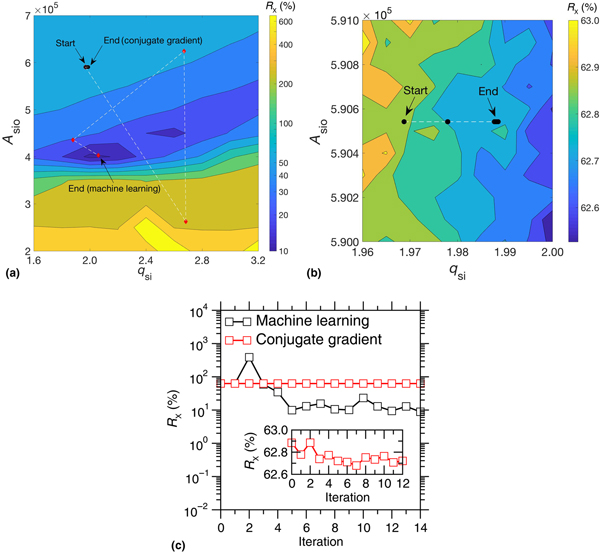
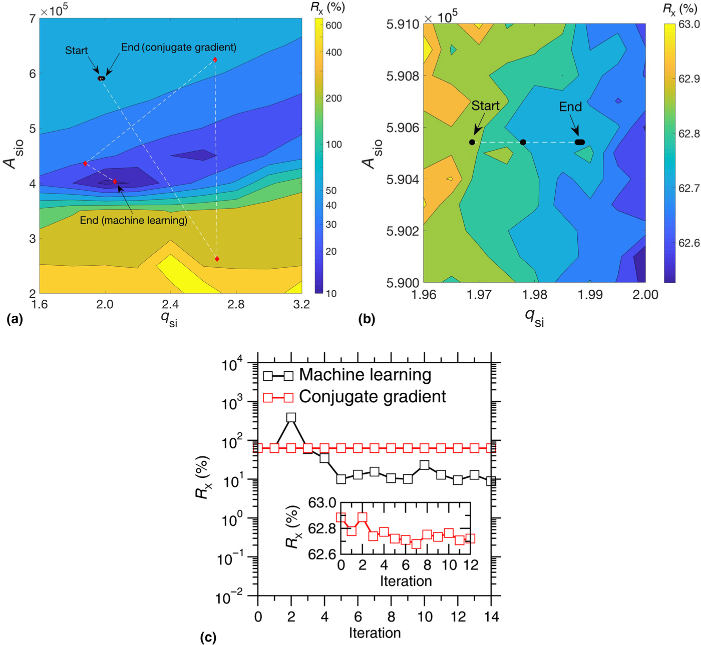
We now discuss the performance of our ML-based optimization method by comparing its ability to identify the global minimum of the cost function with that of the CG method. Here, for illustrative purposes, only two parameters (q Si and A SiO) are optimized in both cases, while the other eight forcefield parameters are kept fixed and equal to those found in the original BKS potential.[Reference van Beest, Kramer and van Santen14] As shown in Fig. 4(a), the cost function R x shows a very rough dependence on the forcefield parameters—wherein the level of roughness appears to increase when upon zooming on the fine details of the landscape [see Fig. 4(b)]. The pathways explored (starting from the same initial point) upon the ML-based and CG-based optimizations in the (q Si, A SiO) space is shown in Fig. 4(a). We observe that the ML-based optimization quickly converges toward the global minimum of the cost function after only five iterations, after which the cost function R x shows a plateau around 10% [see Fig. 4(c)]. This illustrates the efficiency of our optimization technique. In contrast with our ML optimization method, the CG optimization quickly gets “stuck” in a local minimum of the cost function [see Fig. 4(c)] and does not succeed at identifying the global minimum. This highlights the fact that traditional gradient-based optimization methods are not appropriate in the case of such high-roughness function and, hence, are highly biased based on the chosen starting point. Although the efficiency of the CG method could certainly be improved by adjusting some parameters (e.g., the learning rate and step length[Reference Shewchuk17]), such fine-tuning necessarily requires some level of intuition or trial-and-error optimization, which is a clear advantage of the present ML approach.
Comparison between ML and CG optimization. Only the partial charge of the Si atoms q Si and the parameter A SiO are here optimized, while the other eight forcefield parameters are kept fixed. (a) Contour plot showing the cost function R x as a function of q Si and A SiO. The red and black circles indicate the path explored upon ML and CG optimization, respectively. Panel (b) is a zoom-in of the data presented in panel (a) to better observe the path explored upon CG optimization. (c) Evolution of the cost function R x during the ML and CG optimizations. The inset is a zoom-in of the data obtained in the case of CG optimization.
Lessons from the BKS potential
It worth further focusing on the BKS potential[Reference van Beest, Kramer and van Santen14] to establish some general conclusions regarding the development of interatomic forcefields for glassy materials. The well-established BKS potential was parameterized by sequentially optimizing the O–O and Si–O energy terms so as to an isolated SiO4 cluster (saturated by four H atoms) matches with ab initio simulations. Si–Si energy terms were forced to be zero. In addition, the experimental elastic constants of silica were used to discriminate several competing sets of parameters. This suggests that the BKS potential is specifically trained to offer an excellent description of the interatomic potential in the vicinity of its equilibrium position. In detail, the position of the minima of each energy terms is encoded in the geometry of the isolated SiO4 cluster (i.e., the average interatomic distances), while the curvature of the potential energy at the vicinity of the equilibrium position is encoded in the elastic constant. Nevertheless, as detailed in the section “Results,” this optimization scheme tends to overestimate the radial and angular order around Si atoms (see Figs. 2 and 3). This suggests that optimization schemes placing a strong emphasis on describing the shape of the forcefield in the very close vicinity of the equilibrium position may not be appropriate to describe the disordered structure of glasses, which are intrinsically out-of-equilibrium and wherein the atoms are not exactly located at their minimum-energy positions. For instance, the degree of asymmetry of the forcefield is likely to play a key role in governing the structure of disordered materials and may not be efficiently trained by considering only equilibrium structures (e.g., crystals or isolated clusters). This suggests that parameterization methods based on liquid structures (as the present one) may be more appropriate to develop new improved forcefields for complex glasses.
Conclusions
Overall, this study establishes a general and versatile framework to accelerate the parameterization of new, improved empirical forcefields for disordered materials. As shown herein with the example of silica, our method makes it possible to quickly reoptimize previous well-established potentials (e.g., the BKS forcefield). By using, as a reference, some liquid structures prepared by AIMD simulations, our parameterization scheme is better suited for glass modeling than alternative methods based on equilibrium crystal or isolated atomic clusters. Importantly, the use of ML rather than alternative traditional optimization methods (e.g., CG) (i) drastically improves the efficiency of the parameterization procedure, (ii) suppresses the risk of bias resulting from arbitrary choices regarding the starting point of the optimization, and (iii) significantly reduces the role played by “personal intuition” during the parameterization. As a key advantage over alternative conventional methods, the present ML-based parameterization method is highly scalable and, hence, can be used to parameterize multi-component systems (i.e., many forcefield parameters can be optimized simultaneously). Overall, this work establishes an efficient, pragmatic method to develop new improved forcefields for the simulation of complex “real-world” materials—which addresses an immediate concern since more accurate ML-based forcefields that do rely on a predefined functional are unlikely to be available for complex multi-component systems in the near future.
Acknowledgments
This work was supported by the National Science Foundation under Grants No. 1562066, 1762292, and 1826420.