1. Individual-Based Models in Ecology

While the classical models of theoretical ecology take populations as their basic units, a newer approach to ecological modeling explicitly represents organisms and their properties. The model organisms of individual-based models (IBMs) are given locations, behaviors, developmental trajectories, and the possibility of interaction with other organisms and the environment. The dynamic consequences of these models can be investigated using computer simulations.

In their landmark book about the use of IBMs in ecology, Grimm and Railsback explain the theoretical virtues of IBMs as follows: “We are interested in such population-level properties as persistence, resilience, and patterns of abundance over space and time. None of these population-level properties is just the sum of the properties of individuals. Instead, population-level properties emerge from the interactions of adaptive individuals with each other and the environment” (Reference Grimm and Railsback2005, 4). They go on to argue that constructing and analyzing IBMs is the best way to capture the emergence of population-level properties from individual-level properties and interactions.

We can think of these claims as involving a cluster of four closely related theses:

• 1. Ecological phenomena are not mere aggregates of organisms’ properties.

• 2. Ecological phenomena are emergent.

• 3. IBMs can be constructed that demonstrate emergent phenomena.

• 4. IBMs explain emergent phenomena.

These theses are listed in order of increasing controversy. The first seems completely uncontroversial. No one who looks at the complexity of ecological phenomena could imagine that they are mere aggregates. Even though these systems are composed of individual organisms and abiotic features, the interactions between these organisms and features is absolutely essential to the nature of any ecological system.

The second claim is a little more controversial, but when it is understood in a suitably restrained way, few would argue against the claim that many ecological properties are emergent. In particular, a popular analysis of biological emergence comes from Wimsatt’s (Reference Wimsatt1997) test for aggregativity. An aggregative system is one in which the whole is a mere aggregate of its parts, whereas nonaggregative systems display emergent properties that cannot be accounted for by a simple summation of the properties of individual parts. For a system to count as aggregative, Wimsatt argues that the behavior of the system must be invariant under four different types of alterations to its parts: (1) rearrangement, (2) addition or deletion, (3) decomposition and recombination, and (4) linear amplification. Ecological systems almost always fail some, and often fail all four, of Wimsatt’s criteria. For example, a predator/prey system in the world will have properties like spatial structure, a predator satiation level, individual differences in ability to find cover, and so on, which would prevent invariance under rearrangement, addition, or recombination.

A number of authors have criticized Wimsatt’s test as too weak, admitting too many phenomena as emergent (e.g., Humphreys Reference Humphreys1997). Although I have sympathy with these critiques, I think the sense in which ecologists describe their systems as emergent very closely matches Wimsatt’s test. If this restrained sense of emergence is all that ecologists intend, then there is nothing very mysterious about it. Emergence is simply a matter of higher levels of organization having properties that the parts do not have.

The third and fourth theses are more substantial and more controversial, so let’s begin by considering whether IBMs can be constructed that demonstrate emergent phenomena. I think the best way to approach this question is by looking at the kinds of examples that motivate modelers to make such claims.

One of the most well-known IBMs is Craig Reynold’s Boids model of flocking (Reynolds Reference Reynolds and Stone1987). Boids models were originally developed as a way for computer animators to make more realistic populations of birds. It has since been used in computer animation to simulate many different types of coordinated motion including the movement of fish, penguins, and bats. But more important for our purposes, this model can be used to study how bird flocks can cohere without a master controller when each bird follows a simple set of rules.

The model is implemented as follows: a two-dimensional grid is created and populated with boids, the individuals of the model. These boids have a heading along which they travel at constant speed, and the initial headings are set randomly. In each cycle of the model, every boid updates its heading according to three rules:

To implement these three rules, the modeler must create specific implementations of them. Such implementations explicitly define the boundaries and geometry of the virtual space, the definition of a neighborhood, and a notion of distance. Parameters are needed to specify critical angles and distances for each of the three rules. For example, an implementation of the separation rule might say that the boids need to maintain a minimum distance of 2 units, and if they do not, then they adjust their heading by 3 degrees. An implementation of the alignment rule might say that the boid can “see” all of its neighbors in a 3-unit radius, and in each cycle of the model, it should adjust its heading up to 4 degrees in the direction of its neighbors’ average heading.

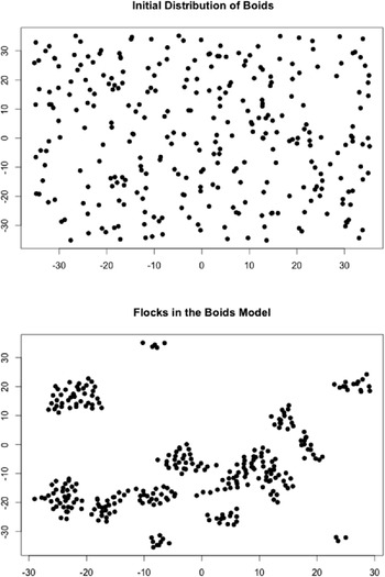
In figure 1, I show an initial, random distribution of boids and the formation of clusters of boids using Wilensky’s (Reference Wilensky1998) implementation of the model. It exhibits the same kind of dynamical flocking patterns as birds or schools of fish. Yet, nowhere in the program is there a description of this behavior; it simply emerges from the way that the model agents interact with one another. Moreover, no one agent is leading the pack. What appears to be purposeful behavior emerges from the interactions.

Figure 1.

Initial random distribution (top) and the formation of flocks (bottom) in a boids model.

Although this is just one example, it is illustrative of what researchers employing IBMs try to do. This model, along with Schelling’s model of segregation, is one of the primary exemplars for fields with names like “Individual Based Ecology” or “Complex Adaptive Systems.” The existence of such models lets us see that the third thesis is true. IBMs are capable of exhibiting or demonstrating emergence.

The most controversial claim about IBMs is that they can explain the emergent phenomena of ecological and other complex systems. Can we really use IBMs to understand the emergence of higher-level ecological phenomena? Not everyone is convinced.

Ecologist Joan Roughgarden gave a very succinct statement of why we might be skeptical of such a claim. She wrote: “I don’t think it’s easy to discern the causation being revealed by an IBM simulation. And if we don’t learn something about causation we don’t learn anything scientifically important. The results of IBMs seem to arise (emerge) by magic. It is not clear how the results are tested and what part of the assumptions is critical to the result. How do we drill down through the computer output to uncover what’s going on that is responsible for the aggregate result?” (personal communication, 2012). Roughgarden’s point is a subtle one. She does not deny that models of underlying mechanisms can be used to help explain higher-level phenomena. Part of the explanation of why, for example, gas expands to fill whatever container it is sealed in has to do with the underlying structure and motion of the gas molecules. What she is arguing is that to explain the emergence of a higher-level phenomenon, you need to explain how the lower-level processes give rise to the higher-level behavior.

Let’s distinguish between explanations of emergent phenomena and explanations of the emergence of phenomena. Call the first group mechanistic explanations and the second emergence explanations. Grimm and Railsback’s fourth thesis is ambiguous between these two readings. If they are speaking about generating mechanistic explanations for higher-level phenomena, then the crucial test is to see whether we can learn about the counterfactual dependence of higher-level properties on lower-level mechanisms. If, however, they mean that IBMs can give us emergence explanations, then we need to be able to “drill down” to the underlying causal structure of the model to see how this gives rise to the higher-level patterns. This is a kind of reductive explanation, which requires connecting the mechanism instantiated in the IBMs with the higher-level phenomenon.

Before proceeding, I want to note that the demand for emergence explanations and the reductionism that this entails need not be part of a general commitment to the explanatory priority of reductive explanation. A blanket commitment to reductionism is compatible with Roughgarden’s desire to see emergence explanations, as is a more liberal view about the nature of explanation that allows for explanations to come in different forms. However, if one wants to give an emergence explanation, to show how the lower-level mechanism gives rise to the higher-level emergent phenomenon, then some kind of reductive explanation has to be constructed.

2. Mechanistic Explanations with IBMs

IBM-based mechanistic explanations allow us to abstract from the details of each and every interaction between individuals (i.e., the actual instantiation of the IBM) and develop a generalized mechanistic understanding of the dependence of higher-level properties and patterns on lower-level mechanistic factors. Although this kind of analysis is not always easy to perform, it is the sort of thing that can be seen in exemplary IBM research.

In order to illustrate how such an analysis works, let’s consider a more biologically realistic example of an IBM drawn from the forestry literature. Before extensive human settlement, much of central Europe was covered by a climax beech forest. This forest had a particular spatial pattern: although most of it was composed of dense growth with a thick canopy, there were patches where the forest was thin, and trees of various species, sizes, and ages filled in.

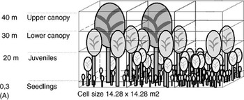
One model that tries to account for this patchiness, along with the vertical structure of forest stands is the BEFORE (BEech FOREst) model (Rademacher et al. Reference Rademacher, Neuert, Grundmann, Wissel and Grimm2004). This model represents the forest as a grid of 14 m² cells and proceeds in time steps whereby each cell on the grid updates its state according to the model’s transition rules. Each cell can represent a location that is composed of beech, pioneer species such as birch, or a mixture of species.

In order to represent height, the BEFORE model stacks four cells vertically on top of each cell of the two-dimensional grid. These vertical cells correspond to the ground (seedling) layer, the juvenile tree layer, the lower canopy, and the upper canopy. Each vertical cell can contain trees of the appropriate height, with trade-offs restricting the total number of trees that can grow at a particular cell on the two-dimensional lattice.

Trees in the upper canopy are represented as having crowns. This allows the model to represent the interaction between crown widths, the sizes of other trees, and the amount of sunlight reaching the forest floor. For example, a single tree that takes up 50% of a cell’s horizontal area will prevent more trees from growing in a given cell than one that takes up 12.5%. Spaces in the upper canopy allow trees in the lower canopy to rapidly grow and fill this space. Spaces in both canopies allow light to reach the understory and promote growth. Further, the model allows an occasional heavy wind to topple the tallest trees and hence to open spaces in the canopy. A simplified representation of the BEFORE model is shown in figure 2.

Figure 2.

Simplified representation of the BEFORE model described in Rademacher et al. (Reference Rademacher, Neuert, Grundmann, Wissel and Grimm2004). Figure courtesy of Volker Grimm.

Through a set of nine main transition rules, BEFORE’s creators attempted to reproduce the dynamical pattern of patch formation and the typical pattern of forest succession (changes in species types and maturity levels) without specifically encoding these dynamics into the model. The transition rules involve development of individual trees, interaction with light, possibility of storm events, and so forth.

Succession patterns involve more than changes in species; they also involve changes in the vertical cross-section of a forest. Early communities contain short plants and trees. By the time a mature beech forest is established, the canopy is very high and the understory is mostly clear. The tallest trees receive all of the sunlight because of this canopy. At the same time, the height of these mature beech trees makes them susceptible to being damaged or killed by powerful windstorms.

Simulations using the BEFORE model generate mosaic patterns of trees, but the most interesting uses of the model are those that show what can generate these mosaic patterns. In particular, the BEFORE model shows that disturbances to the system often lead to local homogenization. For example, when an extremely strong storm that destroys large parts of the upper canopy is unleashed in the model, the forest quickly homogenizes in the damaged locations. “It takes about seven time steps (ca. 100 years) until the effect, or ‘echo’, of the extreme storm event is ‘forgotten’, i.e. no longer detectable in the forest structure and dynamics” (Rademacher et al. Reference Rademacher, Neuert, Grundmann, Wissel and Grimm2004, 360).

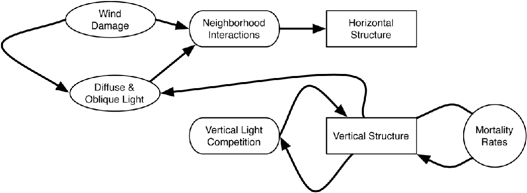
In summarizing the factors responsible for forest structure, Rademacher et al. argue that despite the many variables in the model and the model’s many transition rules, most of the forest structure can be explained by two major factors: vertical light competition and neighborhood interactions. Vertical light competition is primarily responsible for the vertical structure of the forest. It is itself affected by the existing vertical structure of the forest and tree mortality rates. Neighborhood interactions drive the horizontal or mosaic structure of the forest. These interactions are primarily driven by incident diffuse and oblique light, which are themselves affected by vertical structure and wind damage from major storms.

Rademacher et al. discovered that these factors were key to explaining forest structure by engaging in a kind of counterfactual analysis. They systematically altered variables and parameters, holding some fixed and changing others, and looked at the effect it had on synchrony, patchiness, and vertical structure. Their paper lists a total of 16 parameters that were investigated, and they use the outcome of this investigation to determine the most important causal factors.

One way to represent the kind of results summarized above is to construct a causal graph (Pearl Reference Pearl2000; Spirtes, Glymour, and Scheines Reference Spirtes, Glymour and Scheines2000). Although much of the literature has focused on the use of statistics to construct causal graphs from data sets, one can also construct the complete causal graph of an IBM by systematic exploration of the parameter space. In figure 3, I show a causal graph describing the results reported in Rademacher et al. (Reference Rademacher, Neuert, Grundmann, Wissel and Grimm2004). This graph is a summary of what was discovered by analyzing the BEFORE model, and a similar graph could be constructed for any IBM.

Figure 3.

Causal graph showing the major mechanistic relationships in the BEFORE model.

This causal graph of the BEFORE model is clearly the representation of a mechanism. It shows the dependence of horizontal and vertical forest structure on neighborhood interactions and mesolevel properties such as wind damage and incident light. This graph gives us the base from which we can give mechanistic explanations for the forest’s structure. For example, if a bit more detail about the strength and directionality of the connections was filled in, it would let us determine how patchiness increases with increasing wind damage.

In general, IBM-generated causal graphs show the dependence of higher-level, emergent properties on lower-level ones. This kind of mechanistic information is exactly what we need to generate mechanistic explanations for emergent phenomena. But the question still remains: Can IBMs help us to explain the emergence of those higher-level properties? Can we construct the appropriate kind of reductive explanation that shows why the higher-level property emerged from the ensemble of the lower-level ones?

3. Emergence Explanations

We come finally to the question of emergence explanations: reductive explanations that show how emergent phenomena arise from lower-level interactions. As those familiar with the literature about reduction know, strict reductive explanations are very hard to come by. The Nagelian view of reduction as complete derivation of higher-level phenomena from lower-level phenomena finds few examples, even in physics. The most plausible cases of reductive explanations are not direct derivations but instead rely on yet more theory at an intermediate level. This theory, often statistical, connects the underlying physical interactions with the higher-level property. It is worth taking the time to look at one such example in order to consider how difficult it would be to actually create the right kind of reductive explanation.

One area that has long captured the attention of philosophers working on reductive explanations is statistical mechanics (e.g., Nagel Reference Nagel1961; Sklar Reference Sklar1993). This theory connects higher-level thermodynamic properties to lower-level, physical interactions among particles. Part of the reason these explanations are fruitful to study is because there is well-developed theory at both the higher and the lower level, and statistical mechanics shows how statistical principles can connect these theories.

To illustrate this point, we can take one of the simplest examples from statistical thermodynamics: the explanation for how molecular motion gives rise to the macroscopic property of energy. In order to connect molecular motion to total internal energy, the theorist does the following things: first, she enumerates all the possible microstates of the system. Because we are interested in the connection between motion and energy, we enumerate all of the states corresponding to all possible kinetic and potential energy distributions of the particles in the system. This set of microstates is called an ensemble of states.

The next step in the reductive explanation is to calculate the probability distribution of all the states and the energy of each of these states. Finally, we can recover the relevant property (total internal energy) by connecting a statistical operation, simple summation in this case, to the relevant quantity. This last step gives us an expression for the total internal energy of the system (U) as a summation of the energy of each possible microstate multiplied by the probability of that state. The expression is as follows:

To make this expression useful, we need a way of calculating the probability distribution. If we assume that the system is at equilibrium—not undergoing chemical reactions, not exchanging energy outside of the system, and all of the particles are identical—then we can calculate the relevant probabilities using what is called the canonical partition function (McQuarrie and Simon Reference McQuarrie and Simon1997). The expression for this probability can be written as follows:

where

When the appropriate substitutions are made, we now have a procedure that directly links properties of the underlying molecular motion to a high-level property of the system, in this case, total internal energy.

The details are not as important for this article as the basic structure of the procedure. The emergence of high-level, thermodynamic properties was explained by first developing a high-level theory (thermodynamics) along with the low-level theory (mechanics). A further theory (statistical mechanics) showed how statistical properties of the lower-level system correspond to the higher-level properties. It also explains why the high-level properties have the character that they do.

Could something like statistical mechanics be developed for ecology that would connect lower-level biotic and abiotic properties to higher-level ecological properties? As a contingent matter, this is very doubtful, especially at the current stage in the development of theoretical ecology. Part of the appeal of the IBM research program advocated by Grimm and coworkers is that relatively little is known about the nature of the lower-level ecological interactions. IBMs are supposed to be a way of starting to get a handle on these interactions.

Moreover, there have been attempts to apply statistical mechanics-like methods to ecology (e.g., Dewar and Porté Reference Dewar and Porté2008). These studies almost always rely on highly simplified representations of the higher-level patterns and have to adopt what is called the maximum entropy assumption, an idealization that represents the underlying population as being unstructured. Although some impressive results can be obtained using these methods, it is a far cry from showing how the dynamics of actual populations can arise from individual-level interactions. And this would be complicated manyfold if the underlying population interactions were developed using IBMs instead of more traditional models of species abundance.

It is safe to say that we are nowhere near having a statistical mechanics-like theory for ecology. So it is worth considering whether the kind of information encoded in causal graphs can be used for emergence explanations. Will they allow us to make a series of logical or mathematical inferences that connects the variables in the causal graph with the behavioral pattern? Have we “drilled down” and found the mechanism that produces the emergent behavior?

Constructing causal graphs from IBMs gives us important counterfactual information. Such graphs show us how altering a lower-level property can change a higher-level property. However, the essential information required for emergence explanations is missing. Causal graphs do not explain where the higher-level properties come from or why they have the properties they have. Moreover, counterfactual dependence does not necessarily tell us about the kinds of composition relations necessary for constructing emergence explanations. Thus I conclude, tentatively, that IBMs themselves do not generate explanations of emergence. It may well take a third type of model, akin to statistical mechanics, to generate emergence explanations from IBMs.

I suspect that most individual-based modelers recognize that they are not in a position to give emergence explanations, sometimes writing about other potential avenues for developing emergence explanations. For example, in an important methodological article about agent-based modeling (social science IBMs), Joshua Epstein writes that the primary goal of agent-based modeling is generative. The modeler should ask herself, “How could the decentralized local interactions of heterogenous autonomous agents generate the given regularity?” (Epstein Reference Epstein2006, 5). He goes on to discuss what he calls generative sufficiency. “Agent-based models provide computational demonstrations that a given microspecification is in fact sufficient to generate a macrostructure of interest. Agent-based modelers may use statistics to gauge the generative sufficiency of a given microspecification—to test the agreement of real-world and generated macrostructures. … A good fit demonstrates that the target macrostructure—the explanandum … is effectively attainable under repeated application of agent-interaction rules: It is effectively computable by agent society” (8). The core message is that if you can build a model that generates a phenomenon, you have explained it. Epstein explicitly states the converse: “If you didn’t grow it, you didn’t explain its emergence” (8).

I grant that building an IBM can help us explain the mechanisms underlying an emergent phenomenon. But how can showing that a microspecification is sufficient to generate an emergent phenomenon explain the emergence of that phenomenon? It certainly does not show how the microstructure composes to form the emergent phenomenon. Nor does it show that the emergence of the phenomenon was necessary. Building an IBM that exemplifies a certain emergent property simply shows us that the emergent property can be generated from a given microstructure. Although this might contribute to the emergence explanation, it certainly does not constitute one.

Several replies to my skepticism suggest themselves. The first is simple disagreement with my claim that generative sufficiency does not explain the emergence of higher-level phenomena. One might argue that generative sufficiency constitutes a completely satisfying explanation of emergence. This might be especially true in cases in which IBMs gave unanticipated demonstrations. For example, once you have shown that the mosaic structure of European forests depends on diffuse and oblique light, there is nothing further to explain. Asking for an explanation of this dependence is asking for one explanation too many.

While I have some sympathies with this perspective, I ultimately think that it is too pessimistic. We really do have some examples of genuine emergence explanations, such as those in statistical mechanics. Is there any reason to think that some new theoretical approach for linking IBMs to higher-level behaviors cannot be developed? There certainly is no in-principle reason why such an approach could not be developed.

A second objection suggests that reductive explanations of emergence are incoherent because there is something incoherent about interlevel explanation. One way to formulate this argument would be to start with a causal analysis of explanation. This would require interlevel causation in order to have interlevel explanation. But such causation is highly controversial. Craver and Bechtel, for example, argue that “bottom-up causation” is not a real causal relation. Instead, it refers to a hybrid of “constitutive and causal relations in a mechanism, where the constitutive relations are interlevel, and the causal relations are exclusively intralevel” (Craver and Bechtel Reference Craver and Bechtel2007, 547). If we think that all explanations are causal and Craver and Bechtel are correct about the incoherence of interlevel causation, then we might think that emergence explanations are incoherent.

Even if one accepts Craver and Bechtel’s analysis of interlevel causation, the quest to find emergence explanations using IBMs does not run afoul of this critique. In the cases I have discussed, we do not have a specific understanding of the constitutive relations between lower- and upper-level properties. We know, of course, that forests are composed of trees and that the solar flux on the whole forest is composed of light falling on particular plants. But the goal of emergence explanations is to show that such-and-such aspects of individual-level phenomena in such-and-such degrees combine to form the emergent properties.

A final objection is that I am giving up the game too soon, declaring the impossibility of emergence explanations at a very early stage in IBM research. To be clear, I am not saying that emergence explanations are impossible. Indeed, part of the reason that I do not think that Epstein’s analysis of emergence explanations is sufficient is because I think that (1) there are real emergence explanations in science, and (2) IBM proponents propose to give them but (3) have not yet given them. So while I do not think that the IBM research program has delivered on emergence explanations, I remain hopeful.

Does it really matter whether IBMs can deliver emergence explanations? I suppose it depends why one cares about building IBMs. They undoubtedly have many virtues: IBMs allow for a huge amount of representational flexibility. They make it easy to include fluctuations, inhomogeneities, local adaptation, learning, and so forth. And they allow for a kind of modularity, letting theorists easily “plug in” one bit of theory into another (Railsback and Grimm Reference Railsback and Grimm2011). These features assure that IBMs will have an important place in ecological modeling in the future. Moreover, as I have argued throughout this article, IBMs can give us real mechanistic information about lower-level processes and then show that changes in aspects of these mechanisms give rise to changes in population-level phenomena. However, if we want to give emergence explanations for ecological properties, we do not yet know how to generate them with IBMs.