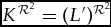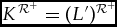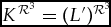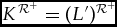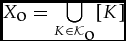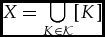



1. INTRODUCTION
How can we explain an agent’s choices? The classical theory of rational choice does so by ascribing to the agent a preference relation over the options – in the simplest case, an ordering. This preference relation explains the agent’s choices if, in every choice context, the agent chooses the most preferred option among the feasible ones.Footnote 1 The choices are then said to be rationalized by the preference relation. When choices involve uncertainty, we must ascribe beliefs as well as preferences to the agent, such that the agent always chooses an expectation-maximizing option, but the logic of the explanation is similar. Though elegant and influential, this theory has some well-known problems:
An empirical problem: It cannot accommodate all empirically documented patterns of choices. As psychologists and behavioural economists have amply shown, people often choose in ways that cannot be naturally rationalized by any preference relation over the options. For example, people are susceptible to framing effects, often satisfice rather than optimize, and follow social norms that are not in line with the constraints of classical rational choice theory (e.g. Camerer et al. Reference Camerer, Loewenstein and Rabin2004). We give some illustrations later.
An explanatory problem: Even when there is a preference relation over the options that rationalizes an agent’s choices, it is far from clear whether this can be viewed as a genuine explanation of those choices. For a start, many economists adopt a behaviouristic interpretation of preferences and treat preference relations merely as formal representations of choices and not as genuinely explanatory. But aside from this concern, when we are asked, ‘why did you choose teaching rather than banking as your career’, simply saying ‘because I preferred one to the other’ is not very illuminating. We are expected to give reasons for our choices, as philosophers and psychologists have long emphasized (e.g. Shafir et al. Reference Shafir, Simonson and Tversky1993; Lenman Reference Lenman and Zalta2011). A better explanation might be that we perceive teaching as a way of making a social contribution and promoting learning, while we perceive banking as a way of making money and supporting the economy’s status quo; and we rank the first bundle of properties more highly than the second.
A predictive problem: A less widely recognized problem is that the classical theory is limited in its ability to predict an agent’s future choices (Bermudez Reference Bermudez2009). If we simply ascribe a preference relation to the agent, based on his or her past choices, then we can predict future choices only in special cases: namely when this preference relation already ranks the options involved. This is only the case when these options are ones the agent has encountered before, unless we can somehow extrapolate the agent’s preferences to them. When the options are genuinely new, this extrapolation is difficult. This limitation is a byproduct of the parsimonious informational basis of classical choice theory.
We introduce a ‘reason-based’ framework for explaining individual choices, which is intended to overcome all of these problems. It is prompted by our diagnosis of a key shortcoming of the classical theory: the lack of an account of how agents perceive the options they are faced with. In the classical theory, options are usually primitives, which are not further unpacked, and agents have preferences over them. In reality, however, each option has numerous properties, and an agent focuses only on some, but not all, of these properties in making his or her choices. Recall the example of teaching versus banking. An agent might perceive the first option as the property bundle ‘contributing to society and promoting learning’ and the second as the property bundle ‘making money and supporting the economy’s status quo’. Our framework captures the idea that agents perceive the options in terms of ‘motivationally salient’ properties. Choices are then made, not based on fixed preferences over options, but based on more fundamental preferences over motivationally salient property bundles (cf. Lancaster Reference Lancaster1966; Gorman Reference Gorman1980).
We lift two common but problematic assumptions. One is that the agents whose choices we seek to explain perceive the options in the same way as we, the modellers, do. In our framework, we can express different hypotheses about how an agent perceives the options, and ask what choice behaviours these hypotheses would predict. A second assumption which we lift is that an agent will always perceive the same options in the same way, irrespective of the choice context. In our framework, an agent’s perception of the options may depend on the context, in the following two ways.
First, the motivationally salient properties may vary from context to context. We call this phenomenon ‘context-variance’. It arguably plays a role in framing effects. Second, the motivationally salient properties may go beyond ‘intrinsic’ properties of the options and include ‘context-related’ properties. Examples are whether an option conforms to a context-specific social norm (e.g. is it polite?), whether it is above average quality among the available options, or whether the choice menu offers luxury options. We call this phenomenon ‘context-relatedness’. It arguably plays a role in sophisticated choice behaviours such as non-consequentialist or norm-following behaviours.
Once we recognize those two kinds of context-dependence, we can explain many non-classical choice behaviours. Finally, the move from options as primitives to options that are perceived as bundles of properties also yields new resources for predicting an agent’s future choices: properties can be recombined in new ways, and an agent’s attitudes towards certain property instantiations in the past can give us evidence for his or her attitudes towards new instantiations of those properties.
Related literature: This paper is related to the large body of work on classical and non-classical choice theory in economics, psychology and philosophy. For an overview of classical choice theory and the rationalization of choices by preferences, see Bossert and Suzumura (Reference Bossert and Suzumura2010). There are, by now, many papers which propose non-classical models of individual choice, prompted by the shortcomings of standard rational choice theory (see e.g. Sen Reference Sen1993; Suzumura and Xu Reference Suzumura and Xu2001; Kalai et al. Reference Kalai, Rubinstein and Spiegler2002; Gaertner and Xu Reference Gaertner and Xu2004; Manzini and Mariotti Reference Manzini and Mariotti2007, Reference Manzini and Mariotti2012; Mandler et al. Reference Mandler, Manzini and Mariotti2012; Cherepanov et al. Reference Cherepanov, Feddersen and Sandroni2013). However, these works do not explain choices in the ‘reason-based’ way developed here or in terms of the two orthogonal kinds of context-dependence we identify.Footnote 2 There are some works discussing variants of one of those two kinds of context-dependence, notably papers by Salant and Rubinstein (Reference Salant and Rubinstein2008), Bernheim and Rangel (Reference Bernheim and Rangel2009), Bossert and Suzumura (Reference Bossert and Suzumura2009) and Bhattacharyya et al. (Reference Bhattacharyya, Pattanaik and Xu2011), as reviewed later.
An important precursor to our approach is Shafir, Simonson, and Tversky’s work on reason-based choice and context-dependent preferences in psychology (e.g. Simonson Reference Simonson1989; Shafir et al. Reference Shafir, Simonson and Tversky1993; Tversky and Simonson Reference Tversky and Simonson1993; for a recent discussion, see de Clippel and Eliaz Reference de Clippel and Eliaz2012). They proposed that ‘when faced with the need to choose, decision makers often seek and construct reasons in order to resolve the conflict and justify their choice’ (Shafir et al. Reference Shafir, Simonson and Tversky1993: 11). Our framework can be viewed as a novel formalization and development of these ideas.
There are also several related works on property-based preferences, the logic of preferences, and preference change. In consumer theory, Lancaster (Reference Lancaster1966) and Gorman (Reference Gorman1980) developed the idea that an agent’s preferences over consumption goods depend on their characteristics. In philosophy, von Wright (Reference von Wright1963) studied the logic of preferences, still influencing current work (e.g. Liu Reference Liu2010); and Pettit (Reference Pettit, Bacharach and Hurley1991) and de Jongh and Liu (Reference de Jongh, Liu, Grüne-Yanoff and Hansson2009) discussed the dependence of an agent’s preferences on properties of the options.
In our own previous work, we developed a model of how reasons, or motivationally salient properties, relate to preferences, and used this model to study preference change (Dietrich and List Reference Dietrich and List2011, Reference Dietrich and List2013a, Reference Dietrich and List2013b). Osherson and Weinstein (Reference Osherson and Weinstein2012) proposed a formal logic of preferences based on reasons. Unlike these earlier papers, the present paper (i) focuses on the explanation of choice, not preference, (ii) treats motivationally salient properties, not as exogenously given, but as endogenously determined by the choice context, and (iii) considers not only ‘intrinsic’ properties of the options, but also properties related to the choice context.
Structure of the paper: In Section 2, we briefly introduce the classical theory of rational choice, our point of departure. In Section 3, we informally describe our framework, followed by a more formal exposition in Section 4. In Section 5, we characterize all choice functions that can be explained in a reason-based way. In Section 6, we discuss some applications. In Section 7, we turn to the prediction of choices in novel contexts.
2. THE CLASSICAL THEORY OF RATIONAL CHOICE
2.1. The basics
We begin by reviewing the basics of classical rational choice theory. The central concept is that of an agent’s choice function. This assigns, to each choice context, the option(s) chosen by the agent in that context. The aim is to explain or ‘rationalize’ a given choice function by ascribing to the agent a preference relation over the options. This ‘rationalization’ is successful if, in each choice context, the agent chooses the most preferred option(s) in that context, according to the ascribed preference relation.
It is natural to view the choice function as the explanandum – the observable object that we seek to explain – and the preference relation as the explanans – the theoretical object that does the explaining. However, as noted in the introduction, many choice theorists avoid using the language of ‘explanation’, because they interpret the preference relation behaviouristically, as a mere representation of the choice function: a convenient way to express its informational content. Elsewhere, we have argued against this behaviouristic interpretation (Dietrich and List Reference Dietrich and List2016).
Formally, the observable primitives of the classical theory are the following:
• A non-empty set X of options. Typical elements are x, y, z, . . .
• A non-empty set
 $\mathcal {K}$ of contexts (sometimes called ‘menus’), where each element $K\in \mathcal {K}$ is a non-empty set K⊆X of feasible options. In the simplest case, $\mathcal {K}$ is the set of all non-empty subsets of X.
• A choice function
$C:\mathcal {K}\rightarrow 2^{X}$, which assigns to each context $K\in \mathcal {K}$ a non-empty set of ‘chosen options’ in K (i.e. C(K)⊆K). If the chosen set C(K) contains more than one option, this means that several options are tied for choice.




The choice function C is rationalizable by a preference relation if there exists a binary relation ≿ on X such that, for all contexts  $K\in \mathcal {K}$,
 $$\begin{equation*}
C(K)=\lbrace x\in K:x\succsim y\text{ for all }y\in K\rbrace \text{.}
\end{equation*}$$
A simple example illustrates these definitions. Here, the set X consists of an apple, a banana and a coconut; the set  $\mathcal {K}$ consists of all non-empty subsets of X; and the choice function C is as follows:
• C({apple, banana, coconut}) = {apple};
• C({apple, banana}) = {apple};
• C({apple, coconut}) = {apple};
• C({banana, coconut}) = {banana};
• C({apple}) = {apple};
• C({banana}) = {banana};
• C({coconut}) = {coconut}.
This choice function can be rationalized by a (complete and transitive) preference relation ≿ which satisfies
 $$\begin{equation*}
\mbox{apple}\succ \mbox{banana}\succ \mbox{coconut}.
\end{equation*}$$
As is standard, ≻ is the strict part of ≿, and ~ is the indifference part.
2.2. When is a choice function rationalizable by a preference relation?
Not all logically possible choice functions can be rationalized by a preference relation. For instance, if an agent chooses an apple from the set {apple, banana, coconut} and a banana from the set {apple, banana}, then no preference relation will rationalize this pattern of choices. To be consistent with the first choice, i.e. C({apple, banana, coconut}) = {apple}, the preference relation would have to rank the apple at least weakly above all three fruits. But then the apple would also have to be chosen from the set {apple, banana}, which contradicts the second choice, i.e. C({apple, banana}) = {banana}.
From the perspective of scientific method, the fact that not all choice functions can be rationalized by a preference relation is good news. It means that the hypothesis that an agent’s choices are based on a preference relation is falsifiable; it is not a tautology (at least once the set of options has been fixed). The following classic result gives necessary and sufficient conditions for a choice function to be rationalizable by a preference relation.
Proposition 1 (Richter Reference Richter and Chipman1971) A choice function C is rationalizable by a preference relation if and only if it satisfies the axiom of Revelation Coherence.
To state that axiom, let us say that an option x is chosen weakly over an option y in context K if x, y ∈ K and x ∈ C(K). Further, x is chosen strictly over y in K if, in addition, y∉C(K).
Revelation Coherence For all contexts  $K\in \mathcal {K}$ and any feasible option x ∈ K, if, for every option y ∈ K, there is a context
 $K^{\prime }\in \mathcal {K}$ in which x is chosen weakly over y, then x ∈ C(K).
Revelation Coherence does not guarantee that the binary relation that rationalizes a given choice function satisfies any further properties such as acyclicity or transitivity. For that, the choice function must satisfy stronger conditions, such as the Weak Axiom of Revealed Preference (e.g. Samuelson Reference Samuelson1948; Bossert and Suzumura Reference Bossert and Suzumura2010). The details need not concern us here. What matters for our purposes is a general point: if, and only if, a choice function satisfies certain structural conditions, it can be rationalized by a preference relation.
2.3. Bounded versus sophisticated rationality
There are at least two familiar kinds of choice behaviours which conflict with the structural conditions just mentioned and which the classical theory therefore cannot accommodate – at least not without significant adjustments.
Cases of bounded rationality: As is empirically well established, human decision-makers often violate conditions such as Revelation Coherence or the Weak Axiom of Revealed Preference due to framing effects, menu-dependent choice, susceptibility to nudges, the use of heuristics, unawareness and other psychological phenomena. For example, a mere redescription of the options can lead to choice reversals. In Tversky and Kahneman’s framing experiments (e.g. Reference Tversky and Kahneman1981), participants reversed their choices over the same pair of options when their description was slightly modified, even though the experimenters were careful not to change any information conveyed. Similarly, policy makers are well aware that subtle changes in the decision environment, such as a change from an ‘opt-out’ to an ‘opt-in’ default in an insurance scheme, can greatly affect people’s choices (Thaler and Sunstein Reference Thaler and Sunstein2008). Decision-makers also often satisfice rather than optimize or use simple heuristics (Gigerenzer et al. Reference Gigerenzer and Todd2000). An example is someone whose rule of thumb for buying a banana is to choose one whose size is above the average of the batch on offer. None of these choices can be rationalized by a preference relation over the options, unless we redescribe the options in a complicated way.
Cases of sophisticated rationality: The structural conditions of the classical theory also fail to accommodate some intuitively rational but sophisticated forms of choice, such as choices based on norm-following or non-consequentialism. For example, a dinner-party guest who never chooses the largest piece of cake offered to him or her for politeness and instead chooses the second largest cannot be rationalized by a preference relation over pieces of cake (Sen Reference Sen1993). The classical theory deems this choice behaviour ‘irrational’, on a par with an ordinary rationality violation. Similarly, consider a professor who votes for a university reform when the dean and president have respected the relevant procedures in the run-up to the vote, but votes against it when there has been a procedural breach. Assume that the reform and its consequences would be the same in both cases. If the options are ‘reform’ and ‘no reform’, we cannot rationalize this choice behaviour by a preference relation. To accommodate it, we would, at least, have to ‘re-individuate’ the options by building some features of the choice context into them.
We suggest that the classical theory’s difficulty in handling these cases, and its inability to distinguish bounded from sophisticated rationality, stems from the lack of a model of how agents perceive the options in any given choice context. When we provide such a model, a unified explanation of many of the challenging phenomena can be given.
3. OUR FRAMEWORK, INFORMALLY EXPLAINED
3.1. The idea of a reason-based explanation of choice
Our basic idea is the following. When an agent chooses between several options in some context, e.g. yoghurts in a supermarket, he or she perceives each option not as a primitive object, but as a bundle of properties. Although each option can have many properties, the agent considers not all of them, but only a subset: the motivationally salient properties. In the supermarket, these may include whether the yoghurt is fruit-flavoured, low-fat, and free from artificial sweeteners, but exclude whether the yoghurt has an odd (as opposed to even) number of letters on its label (an irrelevant property) and whether it has been sustainably produced (a property ignored by many consumers). The agent then makes his or her choice on the basis of a fundamental preference relation over property bundles. He or she chooses one option over another in the given context, e.g. a low-fat cherry yoghurt over a full-fat, sugar-free vanilla yoghurt, if and only if his or her fundamental preference relation ranks the set of motivationally salient properties of the first option, say {low-fat, fruit-flavoured}, above the set of the second, say {full-fat, vanilla-flavoured, artificially sweetened}.
We call an agent’s choice behaviour reason-based explicable if it can be explained in this way. More precisely, a reason-based explanation attributes two things to an agent:
• a motivational salience function, which assigns to each choice context the properties the agent cares about in that context: the ‘motivationally salient’ properties; and
• a fundamental preference relation over bundles of properties.
We call the pair consisting of a motivational salience function and a fundamental preference relation a reasons structure. According to a reason-based explanation, the agent perceives the options in each context through the lens of the motivationally salient properties in that context; and the agent then chooses an option whose bundle of motivationally salient properties he or she most prefers.
Later, we axiomatically characterize all choice functions that admit a reason-based explanation. Technically, reason-based explanation is a new rationalization concept. But given our emphasis on the idea of explaining choices, we use the term ‘explanation’ rather than ‘rationalization’.
3.2. How the context matters
In our framework, the motivationally salient properties that occur in a reasons structure may be of up to three kinds:
• option properties, which options have independently of the choice context and which are thus ‘intrinsic’ to the options;
• relational properties, which options have relative to the context; and
• context properties, which are properties of the context alone.
Examples of option properties are ‘fruit-flavoured’ and ‘low-fat’ (in yoghurts); these depend solely on the yoghurt itself. Examples of relational properties are whether a yoghurt is the only cherry yoghurt on display, or the cheapest; these depend also on the other available yoghurts. Examples of context properties are whether the available yoghurts include premium brands (this depends only on the menu) and whether there is background music (this depends on features of the context over and above the menu).
Reason-based explanations can capture two kinds of context-dependent motivation:
Context-variance: Here, the context affects which properties are motivationally salient, so that the agent cares about different properties in different contexts. For example, some contexts make the agent diet-conscious, others not.
Context-relatedness: Here, the motivationally salient properties in some contexts go beyond option properties and include relational or context properties, so that the agent cares about the context or about how the options relate to it. For example, the agent cares about whether the choice of an option is polite in the given context, whether it is bigger than average, or whether there are luxury options available.
Many non-classical forms of choice can be subsumed under these two kinds of context-dependence. Arguably, bounded rationality, including susceptibility to framing, often involves context-variant motivation. Sophisticated rationality, such as norm-following or non-consequentialism, often involves context-related motivation. By contrast, classical rationality excludes both kinds of context-dependence. Of course, we do not claim that context-variance is always boundedly rational or that context-relatedness is always sophisticated. Our point is that reason-based explanations can be given for a variety of choice behaviours that are not classically rationalizable by a preference relation.
3.3. A common objection
Before we present our framework formally, it is worth addressing one common objection. Since we take agents to perceive options as bundles of motivationally salient properties, a critic might ask why we do not simply define each option as a bundle of motivationally salient properties. Should we not define the set X as the set of all such bundles? A choice context would then be a set of property bundles among which the agent can choose. Everything else would remain classical.
There are, however, three problems with this proposal (see Bhattacharyya et al. Reference Bhattacharyya, Pattanaik and Xu2011 for some similar observations):
• First, we, the modellers, do not know in advance how the agent will perceive each option in a given context. The motivationally salient properties can be inferred, at most, after observing the agent’s choice behaviour.
• Second, an agent may perceive the same option through the lens of different properties in different contexts, for instance when certain properties are motivationally salient in some contexts but not in others. This problem, together with the first, illustrates that, while we may treat options as observable primitives, we cannot equally treat an option’s motivationally salient properties as an observable primitive. The notion of motivational salience is invoked in our explanation of the agent’s choices; it is not part of our pre-theoretic description of those choices.
• Third, the same option can have different properties in different contexts when these properties are relational. For instance, the same piece of cake can be the second-largest in one context and the largest in another, and thus ‘politely choosable’ in the former context, but not in the latter. If we were to speak of two distinct pieces of cake here, we would no longer capture the fact that there is a perfectly intelligible sense in which they are the same, albeit in different contexts.
To address these problems, we must have a way of distinguishing between an option in the ‘objective’ sense, as viewed from the ‘Olympian’ perspective of the modeller, and an option in the ‘subjective’ sense, as perceived by the agent whose choice behaviour we seek to explain. Our framework allows us to draw this distinction. We can think of each element of the original set X as an option in the ‘objective’ sense. And we can think of each option’s bundle of motivationally salient properties in a given context as the option in the ‘subjective’ sense, as perceived by the agent.
4. OUR FRAMEWORK, FORMALLY DEFINED
4.1. Observable primitives
We are now in a position to present our framework formally. The observable primitives are as in the classical theory. We have a non-empty set X of options; a non-empty set  $\mathcal {K}$ of contexts, each of which offers a non-empty set of feasible options (a subset of X); and a choice function
 $C:\mathcal {K}\rightarrow 2^{X}$, which assigns to each context
 $K\in \mathcal {K}$ a non-empty set of chosen options among the feasible ones in K.
We permit only one small (but optional) generalization. Readers who do not like this generalization may ignore it; all our results also hold without it. We no longer require that each context be identified with its set of feasible options. Instead, we merely require that it induce a set of feasible options. Thus a context  $K\in \mathcal {K}$ need not be a subset K⊆X; it must merely pick out such a subset. This permits (but of course does not require) the existence of distinct contexts that offer the same options.
Specifically, each context K could be a pair (Y, λ), where Y is the feasible set (with Y⊆X) and λ is a parameter that specifies some further features of the environment (as in the notion of a ‘frame’ or ‘ancillary condition’ in Salant and Rubinstein Reference Salant and Rubinstein2008 and Bernheim and Rangel Reference Bernheim and Rangel2009; see Section 6.6 below). This parameter could represent a cue given to the agent, a specification of a ‘default’ option, some priming before the choice, the cultural environment, some background music, or the room temperature – even a state of the agent such as ‘sober’ or ‘drunk’. We might distinguish, for instance, between a supermarket with classical music in the background and the same supermarket with pop music, where there is no difference in the goods on offer.
Officially, we write K for the context under our general definition, and [K] for its feasible set, so that [K] is a subset of X, while K need not be. For convenience, we often drop the square brackets and write K for [K], since it is usually unambiguous whether K refers to the context itself or to the feasible set (e.g. in ‘x ∈ K’, K refers to [K]).
4.2. Properties
Our next step is to define properties. At first, we might be tempted to define a property simply as a feature that an option may or may not have. Each property then picks out a subset of X consisting of those options that have the property. The property ‘being a fat-free yoghurt’ can be modelled like this. If X is the set of all possible goods in a supermarket, this property can be identified with the subset of X consisting of all fat-free yoghurts. However, this definition of properties is insufficiently general. As already noted, we want to allow for the possibility that an agent’s choices may be driven by properties that relate to the choice context.
We therefore define properties as features of option-context pairs, i.e. as features of pairs of the form (x, K), where x is an option and K is a choice context. Formally, a property is an abstract object, P, that picks out a subset  $[P]\subseteq X\times \mathcal {K}$ called its extension, consisting of all option-context pairs that ‘have’ or ‘satisfy’ the property; thus properties are binary here. (
 $X\times \mathcal {K}$ is the set of all option-context pairs.Footnote 3) For convenience, we rule out properties that are never satisfied (i.e. [P] is the empty set
 $\varnothing$) and properties that are always satisfied (i.e. [P] is the universal set
 $X\times \mathcal {K}$).
Our definition allows distinct properties to have the same extension. This is useful for capturing framing effects in which the description of a property matters. For example, the properties ‘80% fat-free’ and ‘20% fat’ (in foods) have the same extension but different descriptions and may sometimes prompt different responses. In many applications, however, it suffices to identify properties with their extensions.
We can now formalize the distinction between option properties, context properties and relational properties.
Option properties: These are properties whose possession by an option-context pair depends only on the option, not on the context; they are in this sense ‘intrinsic’ to the option. Examples are ‘fat-free’ and ‘vanilla-flavoured’ (in yoghurts). Formally, P is an option property if
 $$\begin{equation*}
(x,K)\in [P]\Leftrightarrow (x,K^{\prime })\in [P]\text{ for all $x\in X$ and }K,K^{\prime }\in \mathcal {K}\text{.}
\end{equation*}$$
Context properties: These are properties whose possession by an option-context pair depends only on the context, not on the option. Examples are ‘offering more than one feasible option’, ‘offering a Rolls Royce among the feasible options’, and – if contexts specify the choice environment over and above the feasible set – the time (‘it’s evening’), the temperature (‘it’s a hot day’), or a default (‘the status quo is such-and-such’). Formally, P is a context property if
 $$\begin{equation*}
(x,K)\in [P]\Leftrightarrow (x^{\prime },K)\in [P]\text{ for all }x,x^{\prime }\in X\text{ and }K\in \mathcal {K}.
\end{equation*}$$
Relational properties: These are properties whose possession by an option-context pair depends on both the option and the context. Examples are ‘not being the largest piece of cake offered’ and ‘being the most expensive car on the market’. Formally, P is a relational property if it is neither an option property nor a context property.
We call properties that are not option properties context-related and properties that are not context properties option-related. Relational properties are context-related and option-related.
4.3. An example
To illustrate how properties can affect choices, we give an example to which we will refer repeatedly. We introduce this example in a pre-theoretic way, and only later show how it can be explained in our framework. The example concerns the choice of fruit at a dinner party, as in Sen’s well-known story of a polite dinner-party guest (Sen Reference Sen1993).
Let X contain different fruits: apples, bananas, chocolate-covered pears, and possibly others. Each kind of fruit comes in up to three sizes: big, medium and small. A choice context is a non-empty feasible set K⊆X, consisting of fruits currently in the basket (so, in this example, we require only the classical notion of a context). The set of possible contexts is  $\mathcal {K}=2^{X}\backslash \lbrace \varnothing \rbrace$. We consider the following properties:
• ‘big’, ‘medium’, and ‘small’: the option properties of being a big, medium and small fruit, respectively;
• ‘chocolate-offering’: the context property of offering at least one chocolate-covered fruit among the feasible options;
• ‘polite’: the relational property of not being the last available fruit of its kind, i.e. not being the last apple in the basket, the last banana, and so on.
We describe four agents whose choice behaviour we will later explain:
Bon-vivant Bonnie always chooses a largest available fruit. For any K, she chooses
 $$\begin{equation*}
C(K)=\lbrace x\in K:x\text{ is largest in }K\rbrace ,
\end{equation*}$$
where ‘medium’ is larger than ‘small’, and ‘big’ is larger than both other sizes.
Polite Pauline politely avoids choosing the last available fruit of its kind and only secondarily cares about a fruit’s size. For any K, she chooses
 $$\begin{equation*}
C(K)=\lbrace x\in K:x\text{ is largest in }K^{\ast }\text{ if }K^{\ast }\ne \varnothing \text{ and largest in }K\text{ if }K^{\ast }=\varnothing \rbrace ,
\end{equation*}$$
where K* is the set of all fruits in K that are not the last available ones of their kind.
Chocoholic Coco picks any fruit indifferently when no chocolate-covered fruit is available, but otherwise chooses a largest available fruit, because the smell of chocolate makes him hungry. For any K, he chooses
 $$\begin{eqnarray*}
C(K)=\left\lbrace \begin{array}{l@{\quad}l}K & \mbox{if $K$contains no chocolate-covered}\\
& \quad \mbox{fruit,}\\[4pt]
\lbrace x\in K:x\text{ is largest in }K\rbrace & \text{otherwise.} \end{array}\right.
\end{eqnarray*}$$
Weak-willed William makes the same polite choices as Pauline when no chocolate-covered fruit is available, and the same ‘greedy’ choices as Bonnie otherwise, as the smell of chocolate makes him lose his inhibitions. For any K, he chooses
 $$\begin{eqnarray*}
C(K)=\left\lbrace \begin{array}{l@{\quad}l}\mbox{$\lbrace x\in K:x\text{ is largest in }K^{*}\rbrace $} & \mbox{if }\left[\begin{array}{c}\mbox{$K$contains no chocolate-}\\
\mbox{covered fruit and $K^{\ast }\ne \varnothing $} \end{array}\right],\\[5pt]
\lbrace x\in K:x\text{ is largest in }K\rbrace & \text{otherwise}, \end{array}\right.
\end{eqnarray*}$$
where K* is again the set of fruits in K that are not the last available ones of their kind.
4.4. Reason-based explanations
As already anticipated, a choice function admits a reason-based explanation if it can be explained by attributing a reasons structure to the agent. We now make this precise.
The set of potentially relevant properties: We begin by specifying a set  $\mathcal {P}$ of potentially relevant properties. It contains the properties that we, the modellers, have at our disposal when we try to explain the agent’s choices. In our example,
 $\mathcal {P}$ might be the set {big, medium, small, chocolate-offering, polite}. The set
 $\mathcal {P}$ can be partitioned into a set
 $\mathcal {P}_{\text{option}}$ of option properties, a set
 $\mathcal {P}_{\text{context}}$ of context properties, and a set
 $\mathcal {P}_{\text{relational}}$ of relational properties. Our specification of
 $\mathcal {P}$ can be viewed as a background hypothesis to the effect that no properties outside
 $\mathcal {P}$ make a difference to the agent’s choices, while at least some of the properties inside
 $\mathcal {P}$ might do so.Footnote 4 Any subset of
 $\mathcal {P}$ is called a property bundle. For any option x and any context K, we further write
•
$\mathcal {P}(x,K)$ for the bundle of all properties of (x, K), formally $\lbrace P\in \mathcal {P}:(x,K)\in [P]\rbrace ;$•
$\mathcal {P}(x)$ for the bundle of option properties of x, formally $\mathcal {P}(x,K)\cap \mathcal {P}_{\text{option}}$; and•
$\mathcal {P}(K)$ for the bundle of context properties of K, formally $\mathcal {P}(x,K)\cap \mathcal {P}_{\text{context}}$.






A reasons structure: A reasons structure,  $\mathcal {R}$, is a pair (M, ⩾) consisting of:
• A motivational salience function M (formally a function from
$\mathcal {K}$ into $2^{\mathcal {P}}$), which assigns to each context $K\in \mathcal {K}$ a set M(K) of motivationally salient
properties in context K. We require the function M to satisfy an invariance constraint: if two contexts K and K′ are such that $\mathcal {P}(K)=\mathcal {P}(K^{\prime })$, then M(K) = M(K′).• A fundamental preference relation ⩾ over property bundles (formally a binary relation on
$2^{\mathcal {P}}$, on which we initially impose no restrictions). We write > and ≡ for the strict and indifference relations induced by ⩾ .




The function M specifies which properties the agent cares about in each context, and the relation ⩾ specifies how he or she cares about these properties, by ranking different property bundles relative to one another. The invariance constraint on M prevents an empirically ungrounded ascription of motivational differences across contexts. It requires that any two contexts that have the same context properties induce the same motivationally salient properties. So, if we wish to hypothesize that the agent cares about different properties in contexts K and K′, we must be able to point to some difference in context properties that lies behind this motivational difference. Contexts that do not differ in their context properties should be motivationally indistinguishable.
How reasons explain choices: According to the reasons structure  $\mathcal {R}=(M,\ge )$:
• The agent perceives any option x in any context K as the bundle of motivationally salient properties of (x, K), denoted
$x_{K}=\mathcal {P}(x,K)\cap M(K)$.• In any context K, the agent will choose the options which, when perceived in terms of their motivationally salient properties in that context, are ranked most highly by his or her fundamental preference relation, formally
We call
$$\begin{equation*}
C^{\mathcal {R}}(K)=\lbrace x\in K:x_{K}\ge y_{K}\text{ for all }y\in K\rbrace .
\end{equation*}$$
$C^{\mathcal {R}}$ (formally a function from $\mathcal {K}$ into 2X) the choice function induced by $\mathcal {R}$. If ⩾ is insufficiently well-behaved, $C^{\mathcal {R}}(K)$ may be empty for some K, so that $C^{\mathcal {R}}$ may only be an improper choice function.



A choice function  $C:\mathcal {K}\rightarrow 2^{X}$ is reason-based explicable if there exists a reasons structure
 $\mathcal {R}$ (relative to the set
 $\mathcal {P}$ of properties) which induces that choice function (i.e.
 $C=C^{\mathcal {R}}$). We then call
 $\mathcal {R}$ a reason-based explanation for C. Whether a choice function admits a reason-based explanation depends on the underlying set
 $\mathcal {P}$ of properties. We return to the significance of this dependence later.Footnote 5
4.5. Revisiting the example
The four choice functions in our example all admit a reason-based explanation, where  $\mathcal {P}=$ {big, medium, small, chocolate-offering, polite}.
Bon-vivant Bonnie’s choice function can be explained by the reasons structure  $\mathcal {R}=(M,\ge )$ where, for each context K,
 $$\begin{equation*}
M(K)=\lbrace \text{big, medium, small}\rbrace \mbox{ (so $M$ is a constant function)},
\end{equation*}$$
and the preference relation ⩾ places the three singleton property bundles {big}, {medium} and {small} in the linear order satisfying
 $$\begin{equation*}
\lbrace \mbox{big}\rbrace >\lbrace \mbox{medium}\rbrace >\lbrace \mbox{small}\rbrace.^{6}
\end{equation*}$$
For instance, in a context K that offers only a small apple a and a big banana b, Bonnie perceives the two fruits as
 $$\begin{eqnarray*}
a_{K} & =&\mathcal {P}(a,K)\cap M(K)=\lbrace \text{small}\rbrace ,\\
b_{K} & =&\mathcal {P}(b,K)\cap M(K)=\lbrace \text{big}\rbrace \text{,}
\end{eqnarray*}$$
and chooses the banana over the apple, because  $\lbrace \text{big}\rbrace >\lbrace \text{small}\rbrace$.
Polite Pauline’s choice function can be explained by the reasons structure  $\mathcal {R}=(M,\ge )$ where, for each context K,
 $$\begin{equation*}
M(K)=\lbrace \text{big, medium, small, polite}\rbrace \mbox{ (so, again, $M$ is a constant function)},
\end{equation*}$$
and the preference relation ⩾ places the property bundles  $\lbrace \text{big, polite}\rbrace$,
 $\lbrace \text{medium, polite}\rbrace ,$
 $\lbrace \text{small, polite}\rbrace ,$
 $\lbrace \text{big}\rbrace ,$
 $\lbrace \text{medium}\rbrace$ and
 $\lbrace \text{small}\rbrace$ in the linear order satisfying
 $$\begin{equation*}
\lbrace \text{big, polite}\rbrace >\lbrace \text{medium, polite}\rbrace >\lbrace \text{small, polite}\rbrace >\lbrace \text{big}\rbrace>\lbrace \text{medium}\rbrace >\lbrace \text{small}\rbrace \text{.}
\end{equation*}$$
For instance, if only two small apples a and a′ and one big banana b are available in context K, Pauline perceives the three fruits as
 $$\begin{eqnarray*}
a_{K} & =&\mathcal {P}(a,K)\cap M(K)=\lbrace \text{small, polite}\rbrace ,\\
a_{K}^{\prime } & =&\mathcal {P}(a^{\prime },K)\cap M(K)=\lbrace \text{small, polite}\rbrace ,\\
b_{K} & =&\mathcal {P}(b,K)\cap M(K)=\lbrace \text{big}\rbrace \text{,}
\end{eqnarray*}$$
and chooses one of the apples rather than the banana, because  $\lbrace \text{small, polite}\rbrace >\lbrace \text{big}\rbrace$.
Chocoholic Coco’s choice function can be explained by the reasons structure  $\mathcal {R}=(M,\ge )$ where, for each context K,
 $$\begin{eqnarray*}
M(K)=\left\lbrace \begin{array}{l@{\quad}l}\varnothing & \text{if no chocolate-covered fruit is available in $K$,} \\
& \text{i.e. $\text{chocolate-offering}\notin \mathcal {P}(K),$} \\
\lbrace \text{big, medium,} & \text{if a chocolate-covered fruit is available in $K$,} \\
\text{small}\rbrace & \text{i.e. $\text{chocolate-offering}\in \mathcal {P}(K),$} \end{array}\right.
\end{eqnarray*}$$
and the preference relation ⩾ is the same as Bonnie’s, with the additional stipulation that  $\varnothing \equiv \varnothing$. For instance, in a context without a tempting chocolate-covered fruit, Coco picks any fruit indifferently, because he perceives every fruit as the same empty property bundle
 $\varnothing$, where
 $\varnothing \equiv \varnothing$.
Weak-willed William’s choice function can be explained by the reasons structure  $\mathcal {R}=(M,\ge )$ where, for each context K,
 $$\begin{eqnarray*}
M(K)=\left\lbrace \begin{array}{l@{\quad}l}\lbrace \text{big, medium,} & \text{if no chocolate-covered fruit is available in $K$,} \\
\text{small},\mbox{ }\text{polite}\rbrace & \text{i.e. $\text{chocolate-offering}\notin \mathcal {P}(K),$} \\
\lbrace \text{big, medium,} & \text{if a chocolate-covered fruit is available in $K$,} \\
\text{small}\rbrace & \text{i.e. $\text{chocolate-offering}\in \mathcal {P}(K),$} \end{array}\right.
\end{eqnarray*}$$
and the preference relation ⩾ is the same as Pauline’s. So, if context K offers only two small apples a and a′ and one big banana b, then, undisturbed by any smell of chocolate, William perceives these fruits as Pauline does and politely chooses a small apple. If a small chocolate-covered pear is added to the basket, he forgets about politeness and perceives the fruits as Bonnie does, choosing the big banana.
4.6. Two kinds of context-dependence
We say that an agent’s motivation, according to the reasons structure  $\mathcal {R}=(M,\ge )$, is
• context-variant if M is a non-constant function (i.e. M(K) is not the same for all
$K\in \mathcal {K}$), and context-invariant
otherwise;• context-related if the motivationally salient properties that are specified by M include context-related properties (i.e. M(K) contains at least one relational or context property for some
$K\in \mathcal {K}$), and context-unrelated otherwise.


In our example, Polite Pauline displays context-related motivation: the relational property ‘polite’ is motivationally salient for her. Chocoholic Coco displays context-variant motivation: the properties that are motivationally salient for him vary with the context. Weak-willed William displays both kinds of context-dependent motivation: he sometimes cares about the relational property ‘polite’, and he also cares about different properties in different contexts. Bon-vivant Bonnie, finally, illustrates the classical case of fully context-independent motivation.
How do the two kinds of context-dependence affect an agent’s perception of the options? Table 1 shows how a given option x is perceived in context K, depending on which of the two kinds of context-dependence are present. Generally, when both kinds of context-dependence may be present, option x is perceived in context K as  $x_{K}=\mathcal {P}(x,K)\cap M(K)$. This may depend on the context in two places: in the set of properties of the option-context pair (x, K) and in the set of motivationally salient properties in context K. If the agent’s motivation is context-unrelated, the first instance of context-dependence disappears, and
 $\mathcal {P}(x,K)$ can be replaced by
 $\mathcal {P}(x)$. Here, M(K) contains only option properties, so that
 $\mathcal {P}(x,K)\cap M(K)=\mathcal {P}(x)\cap M(K)$. If the agent’s motivation is context-invariant, the second instance of context-dependence disappears, and M(K) can be replaced by a fixed set M of motivationally salient properties. Here, the motivational salience function is constant, so that the first component of the reasons structure (M, ⩾) can be identified with a fixed set M. In the context-independent case, finally, the agent’s perception of option x in context K simplifies to
 $x_{K}=\mathcal {P}(x)\cap M\text{.}$
The agent’s perception of option x in context K

From a classical perspective, agents with context-variant motivation – e.g. whose motivation varies as a result of subtle environmental features like the smell of chocolate – would count as boundedly rational. Bonnie exemplifies the case of classical rationality: her motivation is completely context-independent. Pauline displays sophisticated rational behaviour: she considers not only properties of the options, but also context-related properties, such as politeness. William tries to display the same sophisticated behaviour, but is susceptible to variations in motivation across different contexts. Coco, finally, focuses only on option properties, but, like William, lacks a stable motivation.
5. WHEN DOES A CHOICE FUNCTION ADMIT A REASON-BASED EXPLANATION?
5.1. An axiomatic characterization
In what follows, we state three jointly necessary and sufficient conditions which a choice function  $C:\mathcal {K}\rightarrow 2^{X}$ must satisfy to admit a reason-based explanation. In line with convention, we call these conditions ‘axioms’, though we do not take their satisfaction for granted: it is an empirical question whether an agent’s choice function satisfies them.
Our axioms are each stated relative to a set  $\mathcal {P}$ of properties. As already noted, whether there is a reason-based explanation for a given choice function depends on the set of properties we have at our disposal in constructing this explanation. Our axioms are jointly less restrictive if
 $\mathcal {P}$ is rich than if it is sparse: it is easier to give a reason-based explanation if we have lots of properties at our disposal than if we have only a few.
We begin with an ‘intra-context’ axiom. It says that the agent’s choice in any context does not distinguish between options with the same properties in that context:
Axiom 1 For all contexts  $K\in \mathcal {K}$ and all options x, y ∈ K, if
 $\mathcal {P}(x,K)=\mathcal {P}(y,K)$, then x ∈ C(K)⇔y ∈ C(K).
The second axiom is an ‘inter-context’ axiom. It says that if two contexts offer the same feasible property bundles, the agent chooses options instantiating the same property bundles in those contexts:
Axiom 2 For all contexts  $K,K^{\prime }\in \mathcal {K}$, if
 $\lbrace \mathcal {P}(x,K):x\in K\rbrace =\lbrace \mathcal {P}(x,K^{\prime }):x\in K^{\prime }\rbrace$, then
 $\lbrace \mathcal {P}(x,K):x\in C(K)\rbrace =\lbrace \mathcal {P}(x,K^{\prime }):x\in C(K^{\prime })\rbrace$.Footnote 7
Axioms 1 and 2 jointly imply that choice is based on the properties in  $\mathcal {P}$, but they do not yet imply any maximizing behaviour.Footnote 8 This gap is filled by our third axiom, a variant of Richter’s original axiom of Revelation Coherence, as introduced in Section 2. Unlike Richter’s axiom, ours is formulated at the level of property bundles, not options. We adapt some revealed-preference terminology. For any property bundles S and S′:
• S is feasible in context K if
$S=\mathcal {P}(x,K)$ for some feasible option x ∈ K;• S is chosen in context K if
$S=\mathcal {P}(x,K)$ for some option x ∈ C(K);• S is revealed weakly preferred to S′ (formally S≿CS′) if, in some context, S is chosen while S′ is feasible.Footnote 9


Axiom 3 Whenever a property bundle  $S\subseteq \mathcal {P}$ is feasible in a context
 $K\in \mathcal {K}$ and is revealed weakly preferred to every feasible property bundle in context K, then S is chosen in context K.Footnote 10
Lemma 1 Axiom 3 strengthens Axiom 2.
We can now state our main characterization theorem:
Theorem 1 A choice function C admits a reason-based explanation if and only if it satisfies Axioms 1 and 3 (and therefore 2).Footnote 11
This result holds for every underlying set  $\mathcal {P}$ of properties. We can thus use our framework to assess whether a given choice function admits a reason-based explanation relative to different sets of properties. We can ask: can we explain a car buyer’s choice function by reference to a set of colour-related properties? By reference to a set of status-related properties? Or by reference to a set of speed- and price-related properties? In each case, our axioms, relativized to the appropriate
 $\mathcal {P}$, provide the required conditions.Footnote 12
Reason-based explanations need not be unique. For a given choice function C, there may exist more than one reasons structure  $\mathcal {R}$ such that
 $C=C^{\mathcal {R}}.$ This non-uniqueness can be reduced if we impose further restrictions. In Appendix A, we state some additional characterization results, identifying conditions under which a choice function admits a reason-based explanation with only one, or none, of the two kinds of context-dependence we have discussed. Different reason-based explanations for the same choice function are by no means equivalent: they attribute a different motivational psychology to the agent and may lead to different predictions for novel choice contexts, as shown in Section 7.
5.2. The choice-behavioural falsifiability of reason-based explanations
A key desideratum on any scientific theory is its falsifiability: it must be possible for the theory to be false. A theory that can ‘explain’ everything does not explain anything. Theories of individual choice should be no exception. Choice theorists typically focus on choice-behavioural falsifiability. Although we think that there is no strong scientific reason to restrict the empirical evidence base to choice behaviour alone (excluding e.g. other psychological data), we temporarily follow convention and focus on choice-behavourial falsifiability too (cf. Dietrich and List Reference Dietrich and List2016). How do reason-based explanations fare in this respect?
To answer this question, we must distinguish between two different senses in which reason-based explanations offer a theory of choice. On one interpretation, the specific reason-based explanation that we give for an agent’s choices is our theory. On another interpretation, the reason-based framework in its entirety is our theory.Footnote 13
A specific reason-based explanation as a theory: If an agent’s choice function C is the observable object that we seek to explain, then the specific reasons structure  $\mathcal {R}$ that we attribute to the agent can be viewed as the theory that we offer as an explanation. This theory, which we label
 $T_{\mathcal {R}},$ has the form:
 $$\begin{equation*}
\mathcal {R}\ \text{is the agent's reasons structure (which implies}\ C=C^{\mathcal {R}}).
\end{equation*}$$
This theory is clearly choice-behaviourally falsifiable. In particular, it is falsified if  $\mathcal {R}$ fails to induce C (i.e.
 $C^{\mathcal {R}}\ne C$) and corroborated otherwise (i.e.
 $C^{\mathcal {R}}=C$).
The reason-based framework as a theory: The broader message of our framework is that choices are ‘reason-based’. Applying this to a particular agent, we can view the assertion that the agent’s choice function C admits some reason-based explanation as our theory. Here, the theory, which we label  $T_{\exists \mathcal {R}},$ has the form:
There is some  $\mathcal {R}$ (relative to set
 $\mathcal {P}$ of properties) such that
 $\mathcal {R}$ is the agent’s reasons structure (which implies
 $C=C^{\mathcal {R}}$).
Whether this theory is choice-behaviourally falsifiable depends on the set  $\mathcal {P}$ of properties relative to which it is asserted. If we are sufficiently disciplined in our specification of
 $\mathcal {P}$, then
 $T_{\exists \mathcal {R}}$ is choice-behaviourally falsifiable. With respect to many reasonable specifications of
 $\mathcal {P}$ (e.g.
 $\mathcal {P}=$ {big, medium, small, chocolate-offering, polite} in our example), only some but not all choice functions satisfy our axioms for reason-based explicability. Hence
 $T_{\exists \mathcal {R}}$ is falsified if the agent’s choice function violates our axioms, and corroborated otherwise. Note that
 $T_{\exists \mathcal {R}}$ is equivalent to the conjunction of Axioms 1, 2 and 3. By contrast, if we specify the set
 $\mathcal {P}$ too permissively, then
 $T_{\exists \mathcal {R}}$ may become choice-behaviourally unfalsifiable, as shown in the next subsection.
5.3. The significance of our auxiliary hypothesis
We have noted that the specification of  $\mathcal {P}$ is a crucial auxiliary hypothesis. It deems all properties that are outside that set irrelevant to the agent’s choices. This allows us to rule out reason-based explanations that are too far-fetched – for instance, because they invoke properties which do not plausibly matter psychologically, such as whether there is an even (rather than odd) number of letters on the yoghurt label. Far-fetched explanations, in turn, may not generate reliable predictions of future choices, as discussed later.
Let us illustrate how reason-based explicability will become too permissive and thereby substantively unilluminating if we specify  $\mathcal {P}$ too liberally. Suppose, for instance, we take
 $\mathcal {P}$ to include all properties of the form:
 $$\begin{equation*}
P_{(x,K)}:\mbox{The option-context pair is }(x,K)\mbox{{},}
\end{equation*}$$
where x is an option and K a context in which x is feasible. Let  $\mathcal {P}_{X\times \mathcal {K}}$ be the set of all such maximally specific properties – ‘maximally specific’ because the extension of P (x, K) consists solely of the pair (x, K). It it easy to see that any logically possible choice function C will admit a reason-based explanation whenever
 $\mathcal {P}\supseteq \mathcal {P}_{X\times \mathcal {K}}$. Simply define
 $\mathcal {R}=(M,\ge )$ as follows:
•
$M(K)=\mathcal {P}_{X\times \mathcal {K}}$ for every context K;• for any options x and y and any context K, {P (x, K)} ⩾ {P (y, K)} if and only if x is weakly chosen over y in context K.

In other words, Axioms 1 to 3 become vacuous when  $\mathcal {P}\supseteq \mathcal {P}_{X\times \mathcal {K}}$, so that
 $T_{\exists \mathcal {R}}$ becomes a tautology relative to such a set
 $\mathcal {P}$.
However, the present reasons structure  $\mathcal {R}$ does not provide an illuminating explanation of the choice function C. It accounts for the agent’s choices essentially by saying that the agent chooses option x over option y in context K because he or she fundamentally prefers ‘x in K’ to ‘y in K’. This is as unilluminating as saying ‘I preferred one to the other’ when asked ‘why did you choose teaching rather than banking as your career’. A plausible auxiliary hypothesis would exclude maximally specific properties from the set
 $\mathcal {P}$, unless we have special reasons to include them. Our goal is to identify properties that could make a psychologically plausible difference to the agent’s choices.
5.4. Does the reliance on an auxiliary hypothesis make reason-based explanations ad hoc?
The reliance on an auxiliary hypothesis, encoded by  $\mathcal {P}$, does not render the notion of reason-based explanation ad hoc. It is well known since the works of Duhem and Quine that practically all scientific theories rest on some auxiliary hypotheses. When we test a theory empirically, we are, in effect, testing its conjunction with certain auxiliary hypotheses. Any apparently disconfirming evidence will seldom suffice to falsify the theory by itself, but will falsify it only relative to those auxiliary hypotheses. A stubborn supporter of the theory can always insist that the theory is correct and respond to the evidence by revising the auxiliary hypotheses.
This is famously illustrated by an episode from physics. In the 19th century, it became evident that Mercury’s orbit deviated from the one predicted by Newton’s theory. But rather than admitting that Newton’s theory was falsified by this observation, some scholars, such as the mathematican Urbain Le Verrier, postulated the existence of an additional planet (‘Vulcan’), whose gravitational influence would allow us to accommodate Mercury’s orbit within Newton’s theory. Eventually, of course, Newton’s theory became overwhelmed with recalcitrant evidence, and it was superseded by Einstein’s.
Our claim is that the theory of individual choice is not different from other scientific theories in its reliance on auxiliary hypotheses. We have heard some people suggest (e.g. in response to this paper) that the classical notion of rationalization by a preference relation is purely choice-behavioural and free from auxiliary hypotheses. But this is not true. The key auxiliary hypothesis of the classical theory is its specification of the options. Although these are usually treated as exogenously given, the modeller implicitly asserts an auxiliary hypotheses when specifying them. Just as our notion of reason-based explicability becomes choice-behaviourally unfalsifiable when the set  $\mathcal {P}$ of properties is specified too permissively, so the notion of rationalizability by a preference relation becomes unfalsifiable when the set X of options is specified too fine-grainedly.
To illustrate, let C (a function from  $\mathcal {K}$ into 2X) be any choice function. Simply respecify the options as follows. Let X′ be the set of all pairs of the form (x, K), where x is an option in X and K is a context in which x is feasible. Let
 $\mathcal {K}^{\prime }$ be the result of replacing every original context K in
 $\mathcal {K}$ with
 $$\begin{equation*}
K^{\prime }=\lbrace (x,K):x\in K\rbrace .
\end{equation*}$$
Suppose we now reinterpret the original choice function C as a function C′ from  $\mathcal {K}^{\prime }$ into 2X′ in the following way: for each K′ in
 $\mathcal {K}^{\prime }$, let
 $$\begin{equation*}
C^{\prime }(K^{\prime })=\lbrace (y,K):y\in C(K)\mbox{, where }K\mbox{ is the context in $\mathcal {K}$ to which }K^{\prime }\mbox{ corresponds}\rbrace .
\end{equation*}$$
Then C′ will of course be rationalizable by a preference relation on X′, because each respecified option occurs in precisely one context. And this is so, whether or not the orginal choice function C was rationalizable by a preference relation on X. Crucially, from a choice-behavioural perspective, the functions C and C′ are indistinguishable.
The upshot is this: by representing an agent’s choices in terms of a sufficiently fine-grained set of options, we can always ‘rationalize’ any choice behaviour by a preference relation. And so, the hypothesis that the agent’s choices are rationalizable by a preference relation is choice-behaviourally falsifiable only in conjunction with an auxiliary hypothesis, namely a hypothesis concerning the nature of the options. This issue is often swept under the carpet. (For a notable exception, which includes a more elaborate formal argument for the point we have just made, see Bhattacharyya et al. Reference Bhattacharyya, Pattanaik and Xu2011.) Our framework makes the role played by auxiliary hypotheses transparent.
5.5. Criteria for selecting an explanation in cases of non-uniqueness
We have clarified the sense in which reason-based explanations are choice-behaviourally falsifiable. But we still need to comment on their possible non-uniqueness, relative to choice-behavioural evidence. How can we select a reason-based explanation when the same choice function can be explained in more than one way?Footnote 14 This question matters because different explanations give different accounts of the agent’s motivational psychology, by attributing different reasons structures to him or her. These, in turn, may lead to different predictions for the agent’s future choices, as discussed in Section 7. There are at least three kinds of criteria for deciding which reasons structure  $\mathcal {R}=(M,\ge )$ to attribute to the agent when there are multiple competing ones:
Choice-behavioural difference-making criteria: These require that, as far as possible:
(i) the motivational salience function M deem only those properties motivationally salient that make an observable difference to the agent’s choice behaviour, and
(ii) the fundamental preference relation ⩾ over property bundles be systematically derived from the agent’s choice behaviour.
The goal is to minimize behaviourally ungrounded ascriptions of motivation and fundamental preference. We give one example of such a criterion in Appendix A.3.
Non-choice data: Verbal reports or neurophysiological data, such as responses to property-related stimuli, may help us test hypotheses about
(i) which properties are motivationally salient for the agent in context K and thus belong to M(K),
(ii) which context properties causally affect motivational salience, so that M(K) may vary as contexts K vary in those properties, and
(iii) which property bundles the agent fundamentally prefers to which others.
One might hypothesize that human beings have better conscious access to how they perceive the options in a given context K and therefore to the properties in M(K) than to the context properties that affect what M(K) is (i.e. those properties which, in an empirical study, might be significant explanatory variables for M). Some changes in M(K) might be due to subconscious influences, as in framing or nudging effects. If so, verbal reports may be more relevant to questions (i) and (iii) than to question (ii).
Parsimony criteria: We may try to select a parsimonious reasons structure, where
(i) the sets M(K) of motivationally salient properties generated by M are (a) as small as possible and (b) as unchanging as possible across different K, and
(ii) the relation ⩾ is as sparse as possible (e.g. defined over the fewest possible property bundles).
There may be a trade-off between different dimensions of parsimony. If the sets M(K) contain only few properties, they may not be stable across different K, and vice versa. As shown in Appendix B, we can always formally achieve context-invariance by defining M constantly as the entire set  $\mathcal {P}$ and the fundamental preference relation ⩾ as the revealed preference relation ≿C over property bundles. This makes the sets M(K) unchanging but very large, and hence perhaps psychologically implausible. Conversely, making each M(K) small might require context-variance.
5.6. Classical rationalizability as a special case
Finally, we wish to note that the notion of rationalizability by a preference relation can be recovered as a special case of reason-based explicability. Simply take  $\mathcal {P}=\mathcal {P}_{X}$, defined as the set of all properties of the form
 $$\begin{equation*}
P_{x}:\mbox{ `The option is }x\mbox{{'},}
\end{equation*}$$
where x is an element of X. The extension of each such property Px is the set of all option-context pairs in which x is the option (i.e.  $[P_{x}]=\lbrace (x,K):K\in \mathcal {K}\rbrace$). Then the choice function C is classically rationalizable by a preference relation if and only if it can be explained by the reasons structure
 $\mathcal {R}=(M,\ge )$, where
•
$M(K)=\mathcal {P}_{X}$ for every context K; and• for any options x and y, {Px} ⩾ {Py} if and only if x is weakly chosen over y in some context K.

Of course, this explanation would be unilluminating, as it would always cite an option’s ‘being that option’ as the reason for choosing it. Nonetheless, the present observations help us compare the notion of reason-based explanation with its classical counterpart.
6. SOME APPLICATIONS
To illustrate the generality of our framework, we briefly show how it can accommodate some much-discussed non-classical choice behaviours.
6.1. Framing effects and choice reversals
As illustrated by Tversky and Kahneman’s influential work (e.g. Reference Tversky and Kahneman1981), a framing effect occurs when an agent makes different choices in ‘extensionally equivalent’ contexts, i.e. contexts which ‘objectively’ offer the same options but which are somehow ‘framed’ (described, labelled, presented, . . .) differently. For instance, an agent may reverse his or her choice over public-health programmes, depending on whether these are framed in terms of the number of lives saved or the number of lives lost. Saving m out of n lives (while not saving the remaining n − m) is the same as losing n − m out of n lives (while saving the rest). Yet, people’s choice dispositions may depend on the wording used.
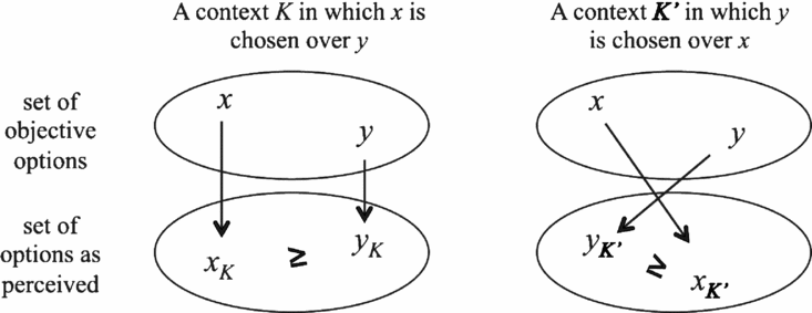
Formally, a framing effect is a special kind of choice reversal. A choice reversal occurs when there are contexts K and K′ and options x and y such that x is chosen over y in K and y is chosen over x in K′, where at least one choice is strict. Suppose  $\mathcal {R}=(M,\ge )$ is the agent’s reasons structure in our framework. Then there may be two possible sources of choice reversals (as well as mixtures of the two).
• Context-variance: Here, the two contexts K and K′ in which a choice reversal occurs induce different sets of motivationally salient properties M(K) ≠ M(K′), where both M(K) and M(K′) contain only option properties.
• Context-relatedness: Here, contexts K and K′ induce the same set of motivationally salient properties M(K) = M(K′), but this set contains some relational or context properties that distinguish between x and y in the two contexts.
In either case, the agent prefers x to y as perceived in context K, and prefers y to x as perceived in context K′, as illustrated in Figure 1.
A choice reversal

Since framing effects are usually thought to be subrational or subconscious, we may take a framing effect to involve a choice reversal whose source is context-variance, not context-relatedness. Whether a choice reversal counts as a framing effect so understood depends on the reasons structure we attribute to the agent. We may then define the frame in each context K simply as the set of context properties of K, formally  $\mathcal {P}(K)$.Footnote 15
6.2. Reference-dependent choice
A widely studied phenomenon is that of reference-dependent choice (e.g. Tversky and Kahneman Reference Tversky and Kahneman1991; Köszegi and Rabin Reference Köszegi and Rabin2006). Here, an agent maximizes an objective function that depends on some ‘reference point’, usually understood as an option that stands out in some way, such as the status quo, a previous choice, or the average among the feasible options. Formally, for each context K, let x* = x*(K) denote the ‘reference point’; this need not be among the feasible options in K. The agent then chooses an option in K which maximizes an objective function that depends on x*.
Our reason-based framework offers two ways of explaining this phenomenon. We can explain it either as involving context-related but context-invariant motivation or as involving context-variant but context-unrelated motivation. In the first case, reference-dependent choice may be interpreted as a sophisticated rational phenomenon, in the second as a subrational one.
Let us give an illustration. Suppose an agent always chooses an option that is as similar as possible to some ‘ideal’, where that ideal depends on the context: the reference point x* = x*(K). For each option x, let d(x, x*) denote its distance from that ideal. One explanation ascribes to the agent a reasons structure (M, ⩾) with context-related but context-invariant motivation. In each context K, the agent cares explicitly about each option’s distance from the context-specific ideal, i.e. M(K) = {P δ: δ ⩾ 0}, where P δ is the relational property of a distance of δ from the ideal.Footnote 16 So, each option x is perceived in context K in a reference-dependent way: xK = {P δ}, where δ = d(x, x*(K)). The agent’s fundamental preference relation then ranks property bundles of the form {P δ} and {P δ′} as follows: {P δ} ⩾ {P δ′}⇔δ ⩽ δ′.
A second explanation is subtly different. Here, in each context K, the agent cares about each option’s distance from some fixed option y. Formally, an option’s distance from some fixed option is an option property: whether x’s distance from y is, say, 10 on some scale does not depend on the context in which we are asking this question, provided y is fixed. Crucially, however, the agent now cares about different such option properties in different contexts. Thus the agent’s motivation is context-variant, but no longer context-related. Formally, for any context K, M(K) = {P δ, y: δ ⩾ 0, y = x*(K)}, where P δ, y is the option property of a distance of δ from y.Footnote 17 The fundamental preference relation then ranks property bundles of the form {P δ, y} and {P δ′, y} as follows: {P δ, y} ⩾ {P δ′, y}⇔δ ⩽ δ′. Whether this second explanation is more adequate than the first depends on the psychological question of whether the agent truly cares about relational properties such as P δ or whether reference-dependent choice happens subconsciously.
6.3. The attraction and compromise effects
We now turn to two further context effects studied in psychology and behavioural economics. They can occur when options are multidimensional objects: jobs, for instance, might have the dimensions of ‘workload’ and ‘salary’. For each dimension, there exists an objective betterness ranking (e.g. on the ‘salary’ dimension, more is better). Formally, let  $X\subseteq \mathbb {R}^{n}$, where n is the number of dimensions. Making a choice is difficult when no feasible option dominates all other feasible options, where dominating an option means being strictly better on at least one dimension and no worse on all others.
The ‘attraction effect’, first reported by Huber et al. (Reference Huber, Payne and Puto1982), ‘refers to the ability of an asymmetrically dominated or relatively inferior alternative, when added to a set, to increase the attractiveness and choice probability of the dominating alternative’ (Simonson Reference Simonson1989: 158). The ‘compromise effect’, introduced by Simonson (Reference Simonson1989: 159), is the phenemenon that an option is more likely to be chosen from a set ‘when it becomes a compromise or middle option in that set’.Footnote 18 We here adopt the following simplifying definitions. We understand the attraction effect as an agent’s tendency to choose an option that dominates as many other feasible options as possible. And we understand the compromise effect as an agent’s tendency to choose an option that is not worst among the feasible options on as many dimensions as possible.
Both effects admit a reason-based explanation, and, as in the case of reference dependence, the explanation can invoke either context-relatedness or context-variance.
The attraction effect: To explain this in a context-related but context-invariant way, let M(K) always be {P 0, P 1, . . .}, where, for each k, Pk is the relational property of dominating exactly k options among the feasible ones in K. The agent then perceives any option x as the singleton property bundle xK = {Pk}, where k is the number of feasible options dominated by x. The fundamental preference relation favours larger numbers of dominated options, i.e. {Pk} ⩾ {P k′}⇔k ⩾ k′. To explain the effect in a context-variant but context-unrelated way, let M(K) be the context-specific set {Py: y ∈ K}, where, for each y in K, Py is the option property of dominating y. Here, different contexts render different such option properties salient, thereby prompting different dominance comparisons. The relation ⩾ ranks property bundles according to the number of options dominated, i.e. S ⩾ S′⇔|S| ⩾ |S′|.
The compromise effect: To explain this in a context-related but context-invariant way, let M(K) always be {P 1, P 2, . . ., Pn}, where, for each i, Pi is the relational property of beating at least one other feasible option on dimension i. The fundamental preference relation ⩾ then ranks property bundles in terms of their size: i.e. the more properties among P 1, P 2, . . ., Pn are satisfied, the better. To explain the effect in a context-variant but context-unrelated way, let M(K) be the context-specific set {P 1, y, P 2, y, . . ., P n, y: y ∈ K}, where, for each i and each y in K, P i, y is the option property of beating y on dimension i. Here, different contexts render different such option properties salient. The relation ⩾ ranks property bundles S according to the number of dimensions i for which S contains at least one property of the form P i, y.
6.4. Checklists or ‘take-the-best’ heuristics
Choices by checklist or ‘take-the-best’ heuristics have received much attention in recent work in economics and psychology. A ‘checklist’ or ‘take-the-best’ decision-maker considers a list of criteria by which the options can be distinguished and places these criteria in some order of importance. For any set of feasible options, the agent first compares the options in terms of the first criterion; if there are ties, he or she moves on to the second criterion; if there are still ties, he or she moves on to the third; and so on. Gigerenzer et al. (Reference Gigerenzer and Todd2000) give several empirical examples of such choice procedures, and de Jongh and Liu (Reference de Jongh, Liu, Grüne-Yanoff and Hansson2009) as well as Mandler et al. (Reference Mandler, Manzini and Mariotti2012) offer relevant formal analyses.
In our framework, we can explain such choice behaviour by a reasons structure  $\mathcal {R}=(M,\ge )$ with a lexicographic fundamental preference relation ⩾ , where property bundles are ranked on the basis of some order of importance over properties. To illustrate, let P 1, P 2, P 3, . . . denote the first, second, third, . . ., properties in this order (assuming a finite
 $\mathcal {P}$). We can then define the fundamental preference relation ⩾ as follows: for any property bundles S 1 and S 2, let S 1 ⩾ S 2 if and only if either S 1 = S 2 or there is some n such that (i) Pn ∈ S 1, (ii) Pn∉S 2, and (iii) S 1∩{P 1, . . ., P n − 1} = S 2∩{P 1, . . ., P n − 1}.
A lexicographic fundamental preference relation can be combined with either context-variant or context-invariant motivation, and with either context-related or context-unrelated motivation. This opens up greater generality than usually acknowledged in discussions of checklists or ‘take-the-best’ heuristics. (For a generalization of the checklist model to variable checklists, see Manzini and Mariotti Reference Manzini and Mariotti2012.)
6.5. Non-consequentialism
A non-consequentialist agent (as discussed e.g. by Suzumura and Xu Reference Suzumura and Xu2001 and Gaertner and Xu Reference Gaertner and Xu2004) makes a choice in a given context not just on the basis of the chosen option itself (the ‘consequence’), but also on the basis of what the choice context is or how each option relates to it (the ‘act of choosing the option’). Any context-related motivation can thus be viewed as a form of non-consequentialism. Many moral theories, such as deontological ones, recommend non-consequentialist forms of choice.
More narrowly, we may describe a non-consequentialist as someone who cares about whether each option is ‘permissible’ or ‘norm-conforming’ in a given context. The relevant criterion may be, for example, politeness, legality, or moral permissibility in the context. Let us introduce a relational property P such that any option-context pair (x, K) satisfies P if and only if the choice of x is deemed permissible or norm-conforming in context K. If P is in every M(K) and the fundamental preference relation ranks property bundles that include P above bundles that do not, the agent will always choose a permissible or norm-conforming option, unless no such option is feasible. Note that this could not generally be modelled without context-related motivation.
6.6. Recent choice-theoretic work on context-dependence
Finally, let us relate our framework to some recent choice-theoretic work on context-dependence. We begin with one pair of contributions, by Salant and Rubinstein (Reference Salant and Rubinstein2008, hereafter S&R) and Bernheim and Rangel (Reference Bernheim and Rangel2009, hereafter B&R), concerning choices that are affected by some external factor. They each describe choice contexts as pairs (Y, λ) of a feasible set Y and an environmental parameter λ, which is the ‘frame’ in S&R or the ‘ancillary condition’ in B&R. In our terms, the two frameworks can be interpreted as models of context-variant rather than context-related motivation. S&R’s frame captures ‘information that is irrelevant in the rational assessment of the alternatives, but nonetheless affects choice’ (p. 1287). B&R’s ancillary condition captures normatively irrelevant features affecting choice.Footnote 19 S&R then focus on the behavioural implications of frame-dependence, B&R on choice-based welfare judgements.Footnote 20
A second pair of contributions, by Bossert and Suzumura (Reference Bossert and Suzumura2009, hereafter B&S) and Bhattacharyya, Pattanaik, and Xu (Reference Bhattacharyya, Pattanaik and Xu2011, hereafter B&P&X), concerns what we would call context-relatedness. B&S assume that, in any given context, each feasible option may or may not be compatible with certain ‘norms’. For instance, picking the last apple might violate a politeness norm. B&S characterize those choice functions which are norm-conditionally rationalizable: there exists a preference relation over options such that, in any context, the agent chooses the most preferred norm-compatible feasible option. In our terms, such a rationalization is ‘partly reason-based’. Each norm generates a context-related property: the property of conforming to it. Every such property is always motivationally salient and deemed desirable. The agent’s choice of a norm-compatible option is then explained by the fact that it has all the norm-conforming properties. However, the choice among the norm-compatible options is explained, not in terms of reasons, but in terms of a preference relation over options. B&P&X, by contrast, model the agent’s perception of the options. Unlike us, they do so, not by invoking properties, but by building some contextual information into the options. To describe Polite Pauline, the options (fruits) would have to be refined by including the information of whether the context offers another fruit of the same kind.Footnote 21 Someone whose choices among refined options are fully rational may nonetheless look irrational if his or her choice function is defined over non-refined options. In sum, we note that while each of the two forms of context-dependence has been studied separately, the previous literature does not offer a joint framework accommodating both.
7. PREDICTING CHOICES IN NOVEL CONTEXTS
Standard choice theory is limited in its ability to predict choices in novel, previously unobserved contexts (see Bermudez Reference Bermudez2009). In most empirical sciences, we make predictions about future (or otherwise unobserved) events, based on past observations. Astronomers predict future solar eclipses or paths of comets based on past trajectories of the relevant celestial bodies; epidemiologists predict future epidemics based on past epidemiological data; and econometricians use past data of the economy to predict its future. In choice theory, by contrast, observations and predictions are often taken to be the same thing: the choice function is the observed and predicted object at once.
Real predictions would have to be about choice contexts outside the observed domain, perhaps with feasible options that the agent has not previously encountered. If we rationalize choices simply by a preference relation on a given set of options, we cannot easily extrapolate this preference relation to new options (though certain extrapolations are sometimes made in consumer theory; cf. Blundell Reference Blundell2005; Varian Reference Varian, Szenberg, Ramrattan and Gottesman2006). On the classical approach, we can make only two rather limited kinds of predictions:
• Any choice function on a given set of contexts can predict choices when the same contexts recur in the future. But here the preference relation does no work, since a not-yet-rationalized choice function entails the same predictions.
• A preference relation might be used to predict choices in ‘new’ contexts when these involve only options over which the preference relation is already defined. We would then predict that the agent will maximize the same preference relation.
These limitations are a consequence of the parsimonious informational basis of classical choice theory. We now show that the additional resources of our reason-based model allow us to move beyond these limitations.Footnote 22
7.1. A framework for predictions
Suppose that we have observed the agent’s choices, not for the entire domain  $\mathcal {K}$ of contexts, but only for some subdomain
 $\mathcal {K_{\mbox{o}}}\subseteq \mathcal {K}$. We call
 $\mathcal {K_{\mbox{o}}}$ the domain of observed contexts. We then write C o to denote the agent’s choice function restricted to that subdomain and call it the observed choice function. Formally, C o is a function from
 $\mathcal {K_{\mbox{o}}}$ into 2X. The agent’s ‘full’ choice function C is an extension of C o to the domain
 $\mathcal {K}$.
The new contexts outside the observed domain (i.e. those in  $\mathcal {K}$\
 $\mathcal {K_{\mbox{o}}}$) may offer options that were not offered by any of the contexts in
 $\mathcal {K_{\mbox{o}}}$. Formally, the set X of all options can be a proper superset of the set X o of previously observed options.Footnote 23
Our goal is to predict as much of the ‘true’ choice function C as possible, on the basis of the observed choice function C o. A choice predictor is a choice function π on some domain  $\mathcal {D\subseteq K}$, where typically
 $\mathcal {\mathcal {\mathcal {K_{\mbox{o}}}\subseteq D}\subseteq K}$. For each K in
 $\mathcal {D}$, π(K) is the predicted choice in context K. The predictor is accurate if it predicts the agent’s choices correctly in all contexts in
 $\mathcal {D}$, i.e. if π(K) = C(K) for all K in
 $\mathcal {D}$.
As noted above, if we were to explain the observed choice function C o simply by attributing a preference relation to the agent, this would leave any options outside the set X o unranked and would therefore allow us to define predictors only for ‘old’ contexts  $K\in \mathcal {K_{\mbox{o}}}$ or for ‘new’ contexts
 $K\not\in \mathcal {\mathcal {K_{\mbox{o}}}}$ containing only ‘old’ options from X o. Our reason-based approach can go further. We define a choice predictor as follows:
• Start from a reasons structure
$\mathcal {R}=(M,\ge )$ for the observed domain $\mathcal {K_{\mbox{o}}}$, where $\mathcal {R}$ explains the observed choice function C o.• Extend this to a reasons structure
$\mathcal {R}^{\prime }=(M^{\prime },\ge )$ for some domain $\mathcal {D}$ with $\mathcal {\mathcal {\mathcal {K_{\mbox{o}}}\subseteq D}\subseteq K}$.• Define a choice predictor on
$\mathcal {D}$ as the choice function $\pi :=C^{\mathcal {R}^{\prime }}$ induced by this extended reasons structure.








By an extension of the reasons structure  $\mathcal {R}=(M,\ge )$ to the domain
 $\mathcal {D}\supseteq \mathcal {K_{\mbox{o}}}$ we mean a reasons structure
 $\mathcal {R}^{\prime }=(M^{\prime },\ge )$ for domain
 $\mathcal {D}$ whose restriction to
 $\mathcal {K_{\mbox{o}}}$ is
 $\mathcal {R}$, i.e. (i) the restriction of the function M′ to the subdomain
 $\mathcal {K_{\mbox{o}}}$ is M, and (ii)
 $\mathcal {R}$ and
 $\mathcal {\mathcal {R}}^{\prime }$ use the same fundamental preference relation ⩾ .Footnote 24
7.2. Cautious, semi-courageous and courageous prediction
We introduce three reason-based choice predictors. Each is based on a reasons structure  $\mathcal {R}=(M,\ge )$ on the domain
 $\mathcal {K_{\mbox{o}}}$ which explains the agent’s observed choices, i.e.
 $C_{\mbox{o}}=C^{\mathcal {R}}$.
Cautious prediction: The cautious predictor (based on  $\mathcal {R}$) is the choice function
 $\pi :=C^{\mathcal {R}^{\prime }}$ induced by the extended reasons structure
 $\mathcal {R}^{\prime }=(M^{\prime },\ge )$ whose domain
 $\mathcal {D}$ consists of every context
 $K\in \mathcal {K}$ such that K offers the same feasible property bundles as some observed context
 $K_{\mbox{o}}\in \mathcal {K}_{\mbox{o}}$:
 $$\begin{equation}
\lbrace \mathcal {P}(x,K):x\in K\rbrace =\lbrace \mathcal {P}(x,K_{\mbox{o}}):x\in K_{\mbox{o}}\rbrace \mathbf {.}
\end{equation}$$
Note that (1) implies  $\mathcal {P}(K)=\mathcal {P}(K_{\mbox{o}})$, so that M′(K) must equal M′(K o), which, in turn, must equal M(K o), because M′ coincides with M for any observed context (in
 $\mathcal {K}_{\mbox{o}}$). By implication, the extension
 $\mathcal {R}^{\prime }$ of
 $\mathcal {R}$ is uniquely defined.
The cautious predictor makes predictions only for choice contexts that offer the same feasible property bundles as some observed context. This ignores the fact that reason-based choices depend only on motivationally salient properties. If we have observed Bonnie’s choices only for some subset  $\mathcal {K}_{\mbox{o}}$ of the set
 $\mathcal {K}$ of all possible fruit baskets, the cautious predictor cannot predict her choices from a ‘new’ fruit basket (in
 $\mathcal {K}\backslash \mathcal {K}_{\mbox{o}}$) that is identical to some ‘old’ basket (in
 $\mathcal {K}_{\mbox{o}}$) in terms of the sizes of available fruit but not in terms of other, non-salient properties. We now introduce a predictor that is based not on entire property bundles but only on bundles of motivationally salient properties.
Semi-courageous prediction: The semi-courageous predictor (based on  $\mathcal {R}$) is the choice function
 $\pi :=C^{\mathcal {R}^{\prime }}$ induced by the extended reasons structure
 $\mathcal {R}^{\prime }=(M^{\prime },\ge )$ whose domain
 $\mathcal {D}$ consists of every context
 $K\in \mathcal {K}$ such that
(i) K has the same context properties as some observed context, i.e.
$\mathcal {\mathcal {P}}(K)=\mathcal {P}(K_{\mbox{o}})$ for some K o in $\mathcal {K}_{\mbox{o}}$ (so that M′(K) = M(K o)), and(ii) the set of options as perceived in K (feasible bundles of motivationally salient properties) is the same as that in some observed context, i.e. {xK: x ∈ K} = {x K′o: x ∈ K′o} for some K′o in
$\mathcal {K}_{\mbox{o}}$.



Note that K o and K′o in clauses (i) and (ii) can be distinct. Although the semi-courageous predictor can predict choices in contexts offering new feasible property bundles, it is still somewhat restrictive. Clause (i) is often unnecessarily demanding. Its role is to tell us how we must define M′(K), namely as M(K o). Sometimes, however, we can infer how to define M′(K) without clause (i). Consider, for example, an agent with context-invariant motivation, according to  $\mathcal {R}$. If we are willing to assume that his or her motivation remains context-invariant in new contexts, we can define M′(K) as unchanged outside
 $\mathcal {K}$. This suggests the following, more general predictor.
Courageous prediction:Footnote 25 We begin with a preliminary definition. In a reasons structure  $\mathcal {R}^{\prime }=(M^{\prime },\ge )$ for some domain
 $\mathcal {D}$, we call a context property P causally relevant if its presence or absence in a context can make a difference to the agent’s set of motivationally salient properties in it, i.e. if there are contexts
 $K,K^{\prime }\in \mathcal {D}$ such that
(cau1) K has property P while K′ does not (or vice versa),
(cau2) K and K′ induce different sets of motivationally salient properties, i.e. M′(K) ≠ M′(K′),
(cau3) K and K′ differ minimally, i.e. there is no context
$K^{\prime \prime }\in \mathcal {D}$ whose set of context properties $\mathcal {P}(K^{\prime \prime })$ is strictly between the sets $\mathcal {P}(K)$ and $\mathcal {P}(K^{\prime })$.Footnote 26


Let  $C\!AU^{\mathcal {R}^{\prime }}$ denote the set of causally relevant context properties in the reasons structure
 $\mathcal {R}^{\prime }$. Two things are worth noting. First, in the special case of context-invariant motivation, no context property is causally relevant. Second, the causally relevant context properties fully determine the agent’s set of motivationally salient properties. Formally:
Proposition 2 Let  $\mathcal {R}^{\prime }=(M^{\prime },\ge )$ be any reasons structure (for some domain
 $\mathcal {D}$ of contexts). Then:
(a)
$\mathcal {R}^{\prime }$ displays context-invariant motivation if and only if $C\!AU^{\mathcal {R}^{\prime }}=\varnothing$.(b) For all K, K′ in
$\mathcal {D}$, if $\mathcal {P}(K)\cap C\!AU^{\mathcal {R}^{\prime }}=\mathcal {P}(K^{\prime })\cap C\!AU^{\mathcal {R}^{\prime }}$ then M′(K) = M′(K′).




The courageous predictor (based on  $\mathcal {R}$) is the choice function
 $\pi :=C^{\mathcal {R}^{\prime }}$ induced by the extended reasons structure
 $\mathcal {R}^{\prime }=(M^{\prime },\ge )$ whose domain
 $\mathcal {D}$ consists of every context
 $K\in \mathcal {K}$ such that
(i*) K has the same causally relevant properties as some observed context, i.e.
$\mathcal {\mathcal {P}}(K)\cap C\!AU^{\mathcal {R}}=\mathcal {P}(K_{\mbox{o}})\cap C\!AU^{\mathcal {R}}$ for some K o in $\mathcal {K}_{\mbox{o}}$; we then define M′(K) as M(K o);Footnote 27 and(ii) the set of options as perceived in K is the same as that in some observed context, i.e. {xK: x ∈ K} = {x K′o: x ∈ K′o} for some K′o in
$\mathcal {K}_{\mbox{o}}$.



Our three predictors are increasingly general:
Remark 1 Given a reason-based explanation  $\mathcal {R}$ of the observed choice function C o,
(a) the cautious predictor extends the observed choice function C o;
(b) the semi-courageous predictor extends the cautious predictor; and
(c) the courageous predictor extends the semi-courageous predictor.Footnote 28
7.3. When is each choice predictor accurate?
It turns out that the accuracy of each predictor depends on whether certain observed patterns in the agent’s choices are robust, i.e. continue to hold in contexts outside  $\mathcal {K}_{\mbox{o}}$.
Theorem 2 Given a reason-based explanation  $\mathcal {R}$ of the observed choice function C o,
(a) the cautious predictor is accurate (i.e. coincides with the true choice function C on its domain) if the true choice function C can be explained by some reasons structure;
(b) the semi-courageous predictor is accurate if the true choice function C can be explained by a reasons structure that is an extension of
$\mathcal {R}$; and(c) the courageous predictor is accurate if the true choice function C can be explained by a reasons structure that is an extension of
$\mathcal {R}$ with the same causally relevant context properties.


Informally, part (a) shows that cautious predictions are accurate if the agent’s choices are robustly reason-based, i.e. reason-based not just in the observed domain  $\mathcal {K}_{\mbox{o}}$ but also in the entire domain
 $\mathcal {K}$. This seems plausible for agents with reasonably stable choice dispositions. Part (b) shows that semi-courageous predictions are accurate if the reasons structure
 $\mathcal {R}$ that explains the agent’s observed choices does so robustly: it not only fits the observed choices, but can be extended so as to explain the agent’s not-yet-observed choices too. This requires that the reasons structure for the observed domain
 $\mathcal {K}_{\mbox{o}}$ be a portion of a reasons structure for the entire domain
 $\mathcal {K}$. Part (c) shows that courageous predictions are accurate if the reasons structure
 $\mathcal {R}$ explains the agent’s choices robustly in an even stronger sense: its extension to new contexts requires no additional causally relevant context properties. So, the reasons structure for
 $\mathcal {K}_{\mbox{o}}$ must be a portion of a reasons structure for
 $\mathcal {K}$ that already identifies all causally relevant context properties.
Whether these robustness assumptions are justified depends, in part, on how rich the domain  $\mathcal {K}_{\mbox{o}}$ of observed contexts is relative to the target domain
 $\mathcal {K}$. Let us explain this in relation to our three-part theorem:
(a) If
$\mathcal {K}_{\mbox{o}}$ is small, then reason-based explicability of the agent’s choices in $\mathcal {K}_{\mbox{o}}$ is only limited evidence for reason-based explicability in $\mathcal {K}$. The smaller $\mathcal {K}_{\mbox{o}}$ is, the less demanding reason-based explicability becomes, and the less it tells us about choices in $\mathcal {K}$. By contrast, if $\mathcal {K}_{\mbox{o}}$ contains a large and representative mix of contexts – e.g. a sizeable ‘random sample’ of contexts from $\mathcal {K}$ – then reason-basedness in $\mathcal {K}_{\mbox{o}}$ may be good evidence for reason-basedness in $\mathcal {K}$.(b) Even if the agent’s choices are robustly reason-based, the reasons structure for
$\mathcal {K}_{\mbox{o}}$ need not be a portion of a reasons structure for $\mathcal {K}$. The set M(K) specified for some observed context K may leave out some property that is needed to explain the agent’s choice in some new context K′ with $\mathcal {P}(K^{\prime })=\mathcal {P}(K)$. If so, a reasons structure for $\mathcal {K}$ could not be an extension of the reasons structure for $\mathcal {K}_{\mbox{o}}$, since it would have to specify the same M(K′) = M(K) for all contexts K′ with $\mathcal {P}(K^{\prime })=\mathcal {P}(K)$. The larger and more representative $\mathcal {K}_{\mbox{o}}$ is, the less likely this problem is to occur.(c) Similar remarks apply to the question of whether the reasons structure for
$\mathcal {K}_{\mbox{o}}$ (even when extendible to one for $\mathcal {K}$) is likely to pick out all context properties that are causally relevant in $\mathcal {K}$. For example, if $\mathcal {K}_{\mbox{o}}$ contains no choice contexts offering luxury goods, then a reasons structure for $\mathcal {K}_{\mbox{o}}$ cannot identify the difference that ‘offering luxury goods’ might make to the agent’s motivation in contexts with that property. A ‘representative’ observed domain $\mathcal {K}_{\mbox{o}}$ reduces the risk of overlooking some context properties that are causally relevant in the target domain $\mathcal {K}$.








8. CONCLUDING REMARKS
Reason-based explanations can make sense of a variety of non-classical choice behaviours in a unified manner and clarify the difference between ‘bounded’ and ‘sophisticated’ deviations from classical rationality. Unlike classical rationalizations of choices by preference relations, reason-based explanations enable us to explain, not only to represent, choices, by identifying the agent’s motivating reasons. Finally, they allow us to predict an agent’s choices in genuinely novel contexts, where no observations have been made. Crucially, different reason-based explanations of the same choice behaviour are not equivalent, since some are more likely than others to extend robustly to new choice contexts and thus to lead to accurate predictions of future choices.
Such robustness is related to psychological adequacy. A psychologically ungrounded explanation of an agent’s observed choices is more likely to fail in novel contexts, because it matches the observations by coincidence rather than for systematic reasons that continue to apply in novel contexts. Psychological adequacy thus matters for the sake of predictive accuracy, regardless of whether it matters for its own sake.
Acknowledgements
This work, previously titled ‘Reason-based rationalization’, was presented many times, beginning with a workshop on ‘Rationalizability and Choice’, LSE, 7/2011. We thank the audiences, the referees, Nick Baigent, Walter Bossert, Richard Bradley, John Broome, Hervé Crès, Johannes Himmelreich, Paola Manzini, Marco Mariotti, Juan Moreno-Ternero, Samir Okasha, Wlodek Rabinowicz, Itai Sher, Kai Spiekermann, Kotaro Suzumura, Laura Valentini, John Weymark and Yongsheng Xu, for comments. Dietrich was supported by a Ludwig Lachmann Fellowship at the LSE and the French Agence Nationale de la Recherche (ANR-12-INEG-0006-01). List was supported by a Leverhulme Major Research Fellowship and the Franco-Swedish Programme in Philosophy and Economics.
A. FURTHER CHARACTERIZATION RESULTS
When does a choice function  $C:\mathcal {K}\rightarrow 2^{X}$ admit a reason-based explanation with only one, or none, of the two kinds of context-dependence? We first discuss the case of reason-based explanation without any context-dependence. We then turn to the case of possibly context-related, but not context-variant motivation. Finally, we address the case of possibly context-variant, but not context-related motivation.
A.1. Reason-based explanation without any context-dependence
To characterize all choice functions that admit a reason-based explanation without any context-dependence, we modify each of our three axioms. We replace Axioms 1 and 2 with variants referring only to option properties:
Axiom 1* For all contexts  $K\in \mathcal {K}$ and all options x, y ∈ K, if
 $\mathcal {P}(x)=\mathcal {P}(y)$, then x ∈ C(K)⇔y ∈ C(K).
Axiom 2* For all contexts  $K,K^{\prime }\in \mathcal {K}$, if
 $\lbrace \mathcal {P}(x):x\in K\rbrace =\lbrace \mathcal {P}(x):x\in K^{\prime }\rbrace$, then
 $\lbrace \mathcal {P}(x):x\in C(K)\rbrace =\lbrace \mathcal {P}(x):x\in C(K^{\prime })\rbrace$.
In our example, Bon-vivant Bonnie, who is ‘classically rational’, satisfies both of these axioms. Chocoholic Coco satisfies Axiom 1* but violates Axiom 2* (to see this, suppose K contains a chocolate-covered pear while K′ does not); and Polite Pauline and Weak-willed William violate even Axiom 1* (they care about a relational property).
We replace Axiom 3 with Richter’s (Reference Richter and Chipman1971) original axiom of Revelation Coherence (as in Section 2), extended to our framework where contexts can go beyond feasible sets.
Axiom 3* For all contexts  $K\in \mathcal {K}$ and any feasible option x ∈ K, if, for every option y ∈ K, there is a context
 $K^{\prime }\in \mathcal {K}$ in which x is chosen weakly over y, then x ∈ C(K).
To state our theorem, call the set of contexts  $\mathcal {K}$closed under cloning if
 $\mathcal {K}$ is closed under transforming any context by adding ‘clones’ of feasible options; formally, whenever a context
 $K\in \mathcal {K}$ contains an option x such that
 $\mathcal {P}(x)=\mathcal {P}(x^{\prime })$ for some other option x′ ∈ X (a clone of x), there is a context
 $K^{\prime }\in \mathcal {K}$ such that K′ = K∪{x′}.Footnote 29
Theorem 3 Given a set of contexts  $\mathcal {K}$ that is closed under cloning, a choice function C admits a reason-based explanation with context-invariant and context-unrelated motivation if and only if it satisfies Axioms 1*, 2*, and 3*.
A.2. Reason-based explanation with context-invariant motivation
We next characterize all choice functions that admit a reason-based explanation with possibly context-related, but not context-variant motivation. Surprisingly, the axioms characterizing this case are the same as those for reason-based explanation simpliciter. Nonetheless, we must not conclude that the restriction to context-invariance is choice-behaviourally irrelevant: it can still affect the prediction of choices in novel contexts.
Before stating our result formally, let us give an illustration. As noted, Chocoholic Coco can be explained – quite intuitively – by the attribution of a reasons structure with context-variant motivation. But a less intuitive explanation is also possible. It invokes a reasons structure  $\mathcal {R}=(M,\ge )$ with context-invariant motivation, at the expense of making this motivation context-related:
• M assigns to each context the same set of motivationally salient properties M = {big, medium, small, chocolate-offering}, instead of letting motivationally salient properties vary with the presence or absence of chocolate;
• ⩾ places any property bundles that do not contain the property ‘chocolate-offering’ in the same indifference class (e.g. {big} ≡ {small}), and ranks property bundles by ‘fruit size’ when they contain one of the size properties together with the property ‘chocolate-offering’ (i.e. {big, chocolate-offering} > {medium, chocolate-offering} > {small, chocolate-offering}).
Generally, two reasons structures  $\mathcal {R}$ and
 $\mathcal {R}^{\prime }$ are behaviourally equivalent if they induce the same (possibly improper) choice function, i.e. if
 $C^{\mathcal {R}}=C^{\mathcal {R}^{\prime }}$.
Proposition 3 Every reasons structure is behaviourally equivalent to one with context-invariant motivation.
Corollary 1 A choice function C admits a reason-based explanation with context-invariant motivation if and only if it admits a reason-based explanation simpliciter.
As a consequence of Proposition 3, Theorem 1 can be re-stated as a characterization of context-invariant reason-based choice:
Theorem 4 A choice function C admits a reason-based explanation with context-invariant motivation if and only if it satisfies Axioms 1 and 3 (and therefore 2).
Of course, the possibility of re-expressing any reason-based explanation in a context-invariant way disappears once we impose further requirements on the attributed reasons structure  $\mathcal {R}$, such as the requirement that motivation be context-unrelated and that it satisfy other simplicity requirements.Footnote 30
A.3. Reason-based explanation with context-unrelated motivation
We finally characterize all choice functions that admit a reason-based explanation with context-unrelated, but possibly context-variant motivation. To do so, we introduce the notion of revealed motivational salience. Informally, a property P is revealed motivationally salient for an agent in context K if its presence or absence in an option makes a difference to the agent’s choices in contexts ‘like’ K, i.e. contexts with the same context properties as K. Choices in contexts with different context properties are irrelevant, since they could stem from different motivationally salient properties. The choice of moisturizer over sunscreen in a cloudy context is no evidence for whether ‘protecting against UV radiation’ is motivationally salient in a sunny context.
Formally, for each context K, let  $\mathcal {K}_{K}$ denote the set of all contexts K′ in
 $\mathcal {K}$ such that
 $\mathcal {P}(K^{\prime })=\mathcal {P}(K)$. Property P is revealed motivationally salient in context K if there are two pairs of property bundles (S, T) and (S′, T′), where (S′, T′) arises from (S, T) by adding or removing P in one of the bundles, such that
(i) S is chosen in some context
$K^{\prime }\in \mathcal {K}_{K}$ where only the property bundles S and T are feasible, and(ii) S′ is not chosen in some context
$K^{\prime \prime }\in \mathcal {K}_{K}$ where only the property bundles S′ and T′ are feasible.


For instance, we could have S = T = S′ = {P, Q} and T′ = {Q}; here property P has been removed from T. This definition of revealed motivational salience is intended only for special domains of contexts (‘diverse’ domains, defined below). For general  $\mathcal {K}$, it is inappropriate, because a general
 $\mathcal {K}$ need not contain the sorts of contexts used in our definition, i.e. contexts with only two feasible property bundles. The general definition is beyond the scope of this paper. We now introduce a weaker version of Axiom 2*:
Axiom 2** For all contexts  $K,K^{\prime }\in \mathcal {K}$, if
 $\lbrace \mathcal {P}(x):x\in K\rbrace =\lbrace \mathcal {P}(x):x\in K^{\prime }\rbrace$and all option properties of options in K (and hence of options in K′) are revealed motivationally salient in both contexts, then
 $\lbrace \mathcal {P}(x):x\in C(K)\rbrace =\lbrace \mathcal {P}(x):x\in C(K^{\prime })\rbrace$.
Loosely speaking, this axiom says that if two contexts offer the same feasible combinations of option properties and if all those option properties are revealed motivationally salient, then the agent chooses options instantiating the same option properties. This immediately suggests context-unrelated motivation, since context-related properties are treated as irrelevant. But the agent’s motivation could still be context-variant, since different option properties might be revealed motivationally salient in different contexts.
We call the set  $\mathcal {K}$ of contexts diverse if it is closed under removing feasible property bundles or option properties: formally, whenever
 $\mathcal {K}$ contains a context in which property bundles S and T are feasible, and O is a set of option properties, then
 $\mathcal {K}$ also contains a context in which only the bundles S\O and T\O are feasible. This condition can be decomposed into the conjunction of two conditions: (i) closure under removing feasible bundles (the special case where
 $O=\varnothing$) and (ii) closure under removing option properties (the special case where the original context offers only two feasible bundles S and T).Footnote 31
Theorem 5 Suppose the set of contexts  $\mathcal {K}$ is diverse (and each option x in X has finitely many option properties). A choice function C admits a reason-based explanation with context-unrelated motivation if and only if it satisfies Axioms 1*, 2**, and 3.
Which reasons structure with context-unrelated motivation explains the agent’s choices under Axioms 1*, 2**, and 3? The most natural candidate is the revealed reasons structure. This is constructed directly from the choice function C and denoted  $\mathcal {R}^{C}=(M^{C},\ge ^{C})$. Here MC(K) is the set of revealed motivationally salient properties in context K, and S ⩾ CT holds if and only if, in some context, an option perceived as S is chosen while an option perceived as T is feasible.
B. PROOFS
This appendix contains all proofs. In Appendix B.1, we prove the results on the explanation of choices (stated in Section 5 and Appendix A). In Appendix B.2, we turn to the results on the prediction of novel choices (stated in Section 7).
Notation. Recall that a reasons structure  $\mathcal {R} =(M,\ge )$ induces, for every context K in the domain of M,
• options-as-perceived, defined by
$x_{K}=\mathcal {P}(x,K)\cap M(K)$ (for x ∈ X) and• a context-specific preference relation ≿K on X, defined by x ≿Ky⇔xK ⩾ yK.

We sometimes write  $x_{K}^{\mathcal {R}}$ for xK and
 $\succsim _{K}^{\mathcal {R}}$ for ≿K to make the reasons structure in question explicit. We also often write MK as an abbreviation for M(K). Recall further that, for property bundles
 $S,T\subseteq \mathcal {P}$, S≿CT means that S is revealed weakly preferred to T; we also write S≿≾CT to mean that S and T are revealed comparable, i.e. that S≿CT or T≿CS.
B.1. The results on reason-based explanation
Proof of Lemma 1. Assume Axiom 3. As in Axiom 2, consider contexts  $K,K^{\prime }\in \mathcal {K}$ such that (*)
 $\lbrace \mathcal {P} (y,K):y\in K\rbrace =\lbrace \mathcal {P}(y^{\prime },K^{\prime }):y^{\prime }\in K^{\prime }\rbrace$. We only show that
 $\lbrace \mathcal {P}(x,K):x\in C(K)\rbrace \subseteq \lbrace \mathcal {P}(x^{\prime },K^{\prime }):x^{\prime }\in C(K^{\prime })\rbrace$, since the converse inclusion (‘⊇’) is analogous. Suppose x ∈ C(K). The property bundle
 $\mathcal {P}(x,K)$ is feasible in context K, hence by (*) also in context K′. It is revealed weakly preferred to all feasible property bundles in context K, hence by (*) also to all feasible property bundles in context K′. So, by Axiom 3, it is chosen in context K′, i.e. belongs to
 $\lbrace \mathcal {P}(x^{\prime },K^{\prime } ):x^{\prime }\in C(K^{\prime })\rbrace$.
 $\blacksquare$
We give no separate proof of Theorem 1, since this result follows from Proposition 3 and Theorem 4, both of which we shall prove.
Proof of Theorem 3. Let  $\mathcal {K}$ be closed under cloning (which we only need in Step 2).
Step 1. Assume C is explicable by a reasons structure with context-invariant and context-unrelated motivation,  $\mathcal {R}=(M,\ge )$, where
 $M\subseteq \mathcal {P}_{\text{option}}$. We leave the proof of Axioms 1* and 2* to the reader and now prove Axiom 3*. It suffices to show that C is rationalizable in the classical sense by a binary relation on X (see Proposition 1). Since
 $\mathcal {R}$ explains C, the choice set C(K) for a context K consists of the ≿K-best option(s) in K, where ≿K is the preference relation on X induced by the reasons structure
 $\mathcal {R}$ for context K. Given the structure’s context-independence (in both senses), options as perceived do not depend on the context (see Section 2.5), and so ≿K does not depend on K; we can write it as ≿. Therefore the choice function C is rationalizable in the classical sense by a binary relation (i.e. ≿).
Step 2. Now assume Axioms 1*, 2* and 3*. Let ≿* be the classical revealed preference relation on X (so ‘x≿*y’ means x is chosen weakly over y in some context). We prove that C is reason-based explicable by (for instance) the following reasons structure with context-invariant and context-unrelated motivation  $\mathcal {R}=(M,\ge )$:
• M is the set
$\mathcal {P}_{\text{option}}$ of all option properties.• For all property bundles
$S,T\subseteq \mathcal {P}$, ‘S ⩾ T’ means that x≿*y for some options x, y ∈ X such that $\mathcal {P} (x)=S$ and $\mathcal {P}(y)=T$.


Under this reasons structure, options are perceived as follows:
 $$\begin{equation}
x_{K}=\mathcal {P}(x,K)\cap M=\mathcal {P}(x)\text{ for all }x\in X\text{ and }K\in \mathcal {K}\text{.}
\end{equation}$$
Clearly, these options-as-perceived do not depend on the context, and so the induced preference relation ≿ (= ≿K) on X also does not depend on the context K.
Let ≿** be the binary relation defined as
 $$\begin{equation*}
x\succsim ^{\ast \ast }y\Leftrightarrow [x\succsim ^{\ast }y\text{ or }\mathcal {P}(x)=\mathcal {P}(y)]\text{ for all }x,y\in X\text{.}
\end{equation*}$$
We have to prove that  $C=C^{\mathcal {R}}$. This follows from three facts:
(i)
$C^{\mathcal {R}}$ is (classically) rationalizable by ≿;(ii) C is (classically) rationalizable by ≿* and by ≿** (and thus, by any relation ≿′ such that ≿* ⊆ ≿′ ⊆ ≿**);
(iii) ≿* ⊆ ≿ ⊆≿**.

Fact (i): This holds by definition of  $C^{\mathcal {R}}$.
Fact (ii): By Proposition 1, Axiom 3* implies that C is rationalizable by some binary relation. One such relation (in fact, the minimal one) is the classical revealed preference relation ≿*, as is easily checked and well-known (see Richter Reference Richter and Chipman1971). Also, ≿** rationalizes C, which can be shown as follows. Fix a context K. We have to show that
 $$\begin{equation*}
C(K)=\lbrace x\in K:x\succsim ^{\ast \ast }y\text{ for all }y\in K\rbrace .
\end{equation*}$$
Since ≿** extends ≿*, C(K)⊆{x ∈ K: x≿**y for all y ∈ K}. Conversely, suppose x ∈ K such that x≿**y for all y ∈ K. We show that x ∈ C(K). If  $\mathcal {P}(z)=\mathcal {P}(x)$ for all z ∈ K, then C(K) = K by Axiom 1* and the fact that
 $C(K)\ne \varnothing$. Thus x ∈ C(K), as required. Now let z ∈ K such that
 $\mathcal {P}(z)\ne \mathcal {P}(x)$. Consider any y ∈ K. We have to show that x≿*y. If
 $\mathcal {P}(y)\ne \mathcal {P}(x)$, this holds by the definition of ≿** and the fact that x≿**y. Now suppose
 $\mathcal {P}(y)=\mathcal {P} (x)$. Note that x≿*z (since x≿**z and
 $\mathcal {P}(z)\ne \mathcal {P}(x)$). So, there is a context
 $\widetilde{K} \in \mathcal {K}$ such that
 $x\in C(\widetilde{K})$. Since
 $\mathcal {P} (y)=\mathcal {P}(x)$ and since
 $\mathcal {K}$ is closed under cloning, there is a context
 $K^{\prime }\in \mathcal {K}$ such that
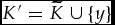 $K^{\prime }=\widetilde{K} \cup \lbrace y\rbrace$. By Axiom 2* and the fact that
 $\lbrace \mathcal {P}(v):v\in \widetilde{K}\rbrace =\lbrace \mathcal {P}(v):v\in K^{\prime }\rbrace$ and
 $x\in C(\widetilde{K})$, we have v ∈ C(K′) for some v ∈ K′ such that
 $\mathcal {P} (v)=\mathcal {P}(x)$. So, by Axiom 1*, x ∈ C(K′). As x ∈ C(K′) and y ∈ K′, we have x≿*y, as required.
Fact (iii): Consider any x, y ∈ X. We have to show that
 $$\begin{equation*}
\text{[}x\succsim ^{\ast }y\Rightarrow x\succsim y\text{] and [}x\succsim y\Rightarrow x\succsim ^{\ast \ast }y\text{].}
\end{equation*}$$
Given that the options-as-perceived take the form (2), we have  $x\succsim y\Leftrightarrow \mathcal {P}(x)\ge \mathcal {P}(y)$. Therefore, we have to prove that
 $$\begin{equation*}
\text{[}x\succsim ^{\ast }y\Rightarrow \mathcal {P}(x)\ge \mathcal {P} (y)\text{] and [}\mathcal {P}(x)\ge \mathcal {P}(y)\Rightarrow x\succsim ^{\ast \ast }y\text{].}
\end{equation*}$$
The first of these two implications holds by definition of ⩾ . As for the second implication, we suppose  $\mathcal {\mathcal {P}}(x)\ge \mathcal {P}(y)$ and claim that x≿**y. If
 $\mathcal {P}(x)=\mathcal {P}(y)$, the claim holds by definition of ≿**. From now on, suppose
 $\mathcal {P}(x)\ne \mathcal {P}(y)$. As
 $\mathcal {P}(x)\ge \mathcal {P}(y)$, there exist x′, y′ ∈ X such that
 $\mathcal {P}(x^{\prime })=\mathcal {P}(x)$,
 $\mathcal {P}(y^{\prime })=\mathcal {P}(y)$, and x′≿*y′. Since x′≿*y′, there is a context
 $K\in \mathcal {K}$ such that x′ ∈ C(K) and y′ ∈ K. Relying twice on the fact that
 $\mathcal {K}$ is closed under cloning, we can choose a context
 $K^{\prime }\in \mathcal {K}$ such that K′ = K∪{x, y}. By Axiom 2* and the fact that
 $\lbrace \mathcal {P} (z):z\in K\rbrace =\lbrace \mathcal {P}(z):z\in K^{\prime }\rbrace$ and x′ ∈ C(K), we have v ∈ C(K′) for some v ∈ K′ such that
 $\mathcal {P} (v)=\mathcal {P}(x^{\prime })$. So, by Axiom 1*, x ∈ C(K′). As x ∈ C(K′) and y ∈ K′, we have x≿*y. So x≿**y, as required.
 $\blacksquare$
Proof of Proposition 3. Consider any reasons structure  $\mathcal {R}=(M,\ge )$. Define a reasons structure with context-invariant motivation
 $\mathcal {R}^{\prime }=(M^{\prime },\ge ^{\prime })$ as follows:
• M′ is any property set such that
$M^{\prime }\supseteq \cup _{K\in \mathcal {K}}(M_{K}\cup \mathcal {P}(K))$ ($=(\cup _{K\in \mathcal {K} }M_{K})\cup \mathcal {P}_{\text{context}}$), for instance $M^{\prime }=\mathcal {P}$;• for any property bundles
$S,T\subseteq \mathcal {P}$, we take ‘S ⩾ ′T’ to mean that there exists a context $K\in \mathcal {K}$ such that $\mathcal {P}(K)=S\cap \mathcal {P}_{\text{context}}=T\cap \mathcal {P} _{\text{context}}$ and S∩MK ⩾ T∩MK.





We prove that  $C^{\mathcal {R}}=C^{\mathcal {R}^{\prime }}$. Consider an arbitrary context
 $K\in \mathcal {K}$; we have to show that
 $C^{\mathcal {R} }(K)=C^{\mathcal {R}^{\prime }}(K)$. We do so by proving that
 $\mathcal {R}$ and
 $\mathcal {R}^{\prime }$ induce the same preference relation on X in context K. Fix options x, y ∈ X. We have to show that
 $x\succsim _{K}^{\mathcal {R} }y\Leftrightarrow x\succsim _{K}^{\mathcal {R}^{\prime }}y$, i.e., writing
 $S=\mathcal {P}(x,K)$ and
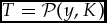 $T=\mathcal {P}(y,K)$, that
 $$\begin{equation*}
S\cap M_{K}\ge T\cap M_{K}\Leftrightarrow S\cap M^{\prime }\ge ^{\prime }T\cap M^{\prime }\text{.}
\end{equation*}$$
We will draw on the fact that (*)  $\mathcal {P}(K)=S\cap \mathcal {P} _{\text{context}}=T\cap \mathcal {P}_{\text{context}}$.
‘⇒’: If S∩MK ⩾ T∩MK, then S ⩾ ′T by (*) and the definition of ⩾ ′; and hence, S∩M′ ⩾ ′T∩M′.
‘⇐’: Now let S∩M′ ⩾ ′T∩M′. By definition of ⩾ ′, there is a context  $K^{\prime }\in \mathcal {K}$ such that
 $\mathcal {P}(K^{\prime })=S\cap \mathcal {P}_{\text{context}} =T\cap \mathcal {P}_{\text{context}}$ and (S∩M′)∩M K′ ⩾ (T∩M′)∩M K′. We deduce two facts. First,
 $\mathcal {P}(K^{\prime })=\mathcal {P}(K)$, where we use (*). Second, S∩M K′ ⩾ T∩M K′, using the fact that M K′⊆M′. The first fact implies that M K′ = MK (by definition of a reasons structure). This and the second fact jointly imply that S∩MK ⩾ T∩MK, as required.
 $\blacksquare$
Before proving Theorem 4, we first show that Axioms 1 and 3 can be jointly summarized in the following axiom:
Axiom 3 $^{\text{+}}$. For any option x in any context
 $K\in \mathcal {K}$, if the property bundle
 $\mathcal {P}(x,K)$ is revealed weakly preferred to
 $\mathcal {P}(y,K)$ for all options y in K, then x ∈ C(K).
Lemma 2 Axioms 1 and 3 are jointly equivalent to Axiom 3 $^{\text{+}}$.
Proof.‘⇐’: First assume Axioms 1 and 3. As in Axiom 3 $^{\text{+}}$, let
 $K\in \mathcal {K}$ and x ∈ K such that
 $\mathcal {P}(x,K)\succsim ^{C}\mathcal {P}(y,K)$ for all y ∈ K. By Axiom 3,
 $\mathcal {P}(x,K)$ is chosen in context K. So, C(K) contains some x′ such that
 $\mathcal {P}(x^{\prime },K)=\mathcal {P}(x,K)$. Thus x ∈ C(K) by Axiom 1.
‘⇒’: Now assume Axiom 3 $^{\text{+}}$. Axiom 3 is obvious. As for Axiom 1, let
 $K\in \mathcal {K}$ and x, y ∈ K such that
 $\mathcal {P} (x,K)=\mathcal {P}(y,K)$. We only show that x ∈ C(K)⇒y ∈ C(K); the converse implication is analogous. Let x ∈ C(K). Then the property bundle
 $\mathcal {P}(x,K)$ is revealed weakly preferred to each feasible property bundle in context K. The same is thus true of the property bundle
 $\mathcal {P}(y,K)$ (
 $=\mathcal {P}(x,K)$). So y ∈ C(K) by Axiom 3
 $^{\text{+}}$.
 $\blacksquare$
Proof of Theorem 4. Step 1. Suppose that a reasons structure with context-invariant motivation, (M, ⩾), explains C. We have to prove Axioms 1 and 3. It suffices to show Axiom 3 $^{\text{+}}$ by Lemma 2. As in Axiom 3
 $^{\text{+}}$, consider a context
 $K\in \mathcal {K}$ and an option x ∈ K such that
 $\mathcal {P}(x,K)\succsim ^{C}\mathcal {P}(y,K)$ for each y ∈ K. We must show that x ∈ C(K), i.e., since (M, ⩾) explains C, that
 $$\begin{equation}
\mathcal {P}(x,K)\cap M\ge \mathcal {P}(y,K)\cap M
\end{equation}$$
for all y ∈ K. Consider any y ∈ K. Since  $\mathcal {P}(x,K)\succsim ^{C}\mathcal {P}(y,K)$, there exist
 $K^{\prime }\in \mathcal {K}$ and x′, y′ ∈ K′ (which may depend on y) such that (i)
 $\mathcal {P}(x^{\prime },K^{\prime })=\mathcal {P}(x,K)$ and
 $\mathcal {P} (y^{\prime },K^{\prime })=\mathcal {P}(y,K)$, and (ii) C(K′) contains x′. Given (ii) and the fact that (M, ⩾) explains C, we have
 $$\begin{equation*}
\mathcal {P}(x^{\prime },K^{\prime })\cap M\ge \mathcal {P}(y^{\prime },K^{\prime })\cap M.
\end{equation*}$$
By (i), this implies (3), as required.
Step 2. Now assume Axioms 1 and 3. We show that C is explicable for instance by the (very special) reasons structure with context-invariant motivation  $(M,\ge )=(\mathcal {P},\succsim ^{C})$, for which (i) all properties are always motivationally salient, and (ii) ⩾ is the relation of revealed weak preference. To show this, let
 $K\in \mathcal {K}$ and x ∈ K. We must show that
 $$\begin{equation*}
x\in C(K)\Leftrightarrow [\mathcal {P}(x,K)\cap M\ge \mathcal {P}(y,K)\cap M\text{ for all }y\in K]\text{,}
\end{equation*}$$
or equivalently, given our special definitions of M and ⩾ , that
 $$\begin{equation*}
x\in C(K)\Leftrightarrow [\mathcal {P}(x,K)\succsim ^{C}\mathcal {P} (y,K)\text{ for all }y\in K]\text{.}
\end{equation*}$$
The right-hand side of this equivalence implies that x ∈ C(K) by Axiom 3 $^{\text{+}}$, where this axiom holds by Lemma 2. Conversely, if x ∈ C(K), then the right-hand side holds by the definition of the revealed preference relation ≿C.
 $\blacksquare$
We now prove Theorem 5.Footnote 32 The proof rests on three key lemmas. They draw on the revealed reasons structure (MC, ⩾C) defined in Appendix A.
Lemma 3 Assume  $\mathcal {K}$ is diverse. If a choice function on
 $\mathcal {K}$ is explicable by a reasons structure (M, ⩾), then MC(K)⊆M(K) for all contexts
 $K\in \mathcal {K}$.
Proof. Assume  $\mathcal {K}$ is diverse and (M, ⩾) explains C. Suppose
 $K\in \mathcal {K}$ and P ∈ MCK. We show that P ∈ MK. Since P ∈ MCK, we can pick a pair of bundles (S, T) and another pair (S′, T′) arising from (S, T) by adding or removing P in one bundle such that
• in a context
$K^{\ast }\in \mathcal {K}$ with $\mathcal {P}(K^{\ast })=\mathcal {P}(K)$, S is chosen and only S and T are feasible; hence, S∩M K* ⩾ T∩M K*;• in a context K** with
$\mathcal {P}(K^{\ast \ast } )=\mathcal {P}(K)$, S′ is not chosen and only S′ and T′ are feasible; hence, $S^{\prime }\cap M_{K^{\ast \ast }} \not\ge U\cap M_{K^{\ast \ast }}$ for some U ∈ {S′, T′}.




Further, as  $\mathcal {K}$ is diverse,
• in a context K*** with
$\mathcal {P}(K^{\ast \ast \ast })=\mathcal {P}(K)$, S′ is the only feasible bundleFootnote 33 (and is thus chosen); hence, S′∩M K*** ⩾ S′∩M K***.

Since  $\mathcal {P}(K^{\ast })=\mathcal {P}(K^{\ast \ast })=\mathcal {P} (K^{\ast \ast \ast })=\mathcal {P}(K)$, we have M K* = M K** = M K*** = MK. So the three bullet points imply that
 $$\begin{equation*}
S\cap M_{K}\ge T\cap M_{K}\text{ and }S^{\prime }\cap M_{K}\not\ge T^{\prime }\cap M_{K}.
\end{equation*}$$
This is only possible if
 $$\begin{equation*}
S\cap M_{K}\ne S^{\prime }\cap M_{K}\text{ or }T\cap M_{K}\ne T^{\prime }\cap M_{K}.
\end{equation*}$$
In each of these two cases, P must belong to MK.  $\blacksquare$
Lemma 4 Assume  $\mathcal {K}$ is diverse (and
 $\left|\mathcal {P} (x)\right|<\infty$ for all x ∈ X). If Axioms 1* and 2** hold, then
 $M_{K}^{C}\subseteq \mathcal {P}_{\text{option}}$ for all
 $K\in \mathcal {K}$, i.e., the revealed reasons structure has context-unrelated motivation.
Proof. Assume  $\mathcal {K}$ is diverse and
 $\left|\mathcal {P}(x)\right|<\infty$ for all x ∈ X. For transparency, the axioms will be added only where needed. Let
 $K\in \mathcal {K}$, and assume for a contradiction that
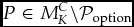 $P\in M_{K}^{C}\backslash \mathcal {P}_{\text{option}}$. As P ∈ MCK, we can choose a pair of bundles (S, T) and another pair (S′, T′) arising from (S, T) by adding or removing P in one bundle such that
(*) in a context
$K^{\ast }\in \mathcal {K}$ with $\mathcal {P}(K^{\ast })=\mathcal {P}(K)$, only S and T are feasible and S is chosen,(**) in a context K** with
$\mathcal {P}(K^{\ast \ast })=\mathcal {P}(K)$, only S′ and T′ are feasible and S′ is not chosen.



Claim 1: There exist
• a context K + in which only the bundles
$S\backslash (\mathcal {P} _{\text{option}}\backslash M_{K}^{C})$ and $T\backslash (\mathcal {P} _{\text{option}}\backslash M_{K}^{C})$ are feasible and the former bundle is chosen, and• a context K − in which only the bundles
$S^{\prime }\backslash (\mathcal {P}_{\text{option}}\backslash M_{K}^{C})$ and $T^{\prime } \backslash (\mathcal {P}_{\text{option}}\backslash M_{K}^{C})$ are feasible and the former bundle is not chosen.
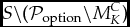
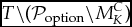


Let P 1, . . ., Pm (m ∈ {0, 1, 2, . . .}) be all the option properties in S or T which are not revealed motivationally salient. There are only finitely many such properties because the set of these option properties is  $(S\cup T)\cap \mathcal {P}_{\text{option}}\backslash M_{K}^{C}$, which is included in the union of the finite sets
 $S\cap \mathcal {P}_{\text{option}}$ and
 $T\cap \mathcal {P}_{\text{option}}$. As
 $\mathcal {K}$ is diverse, it contains a context in which only the bundles S\{P 1} and T\{P 1} are feasible; in that context S\{P 1} is chosen by (*) and the fact that
 $P_{1}\not\in M_{K}^{C}$ .Footnote 34 Next, by an analogous argument, there is a context in which only the bundles S\{P 1, P 2} and T\{P 1, P 2} are feasible and in which S\{P 1, P 2} is chosen. After m such property-removal steps, we reach a context in which only
 $S\backslash \lbrace P_{1},\ldots,P_{m}\rbrace =S\backslash (\mathcal {P}_{\text{option}}\backslash M_{K}^{C})$ and
 $T\backslash \lbrace P_{1},\ldots,P_{m}\rbrace =T\backslash (\mathcal {P} _{\text{option}}\backslash M_{K}^{C})$ are feasible and the former bundle is chosen. This proves the claim within the first bullet point. The claim within the second bullet point is proved by a similar property-removal argument, but using (**) instead of (*). This completes the proof of Claim 1.
In what follows, K + and K − are contexts as in Claim 1.
Claim 2: Under Axiom 2**,  $\lbrace \mathcal {P}(x):x\in C(K_{+} )\rbrace =\lbrace \mathcal {P}(x):x\in C(K_{-})\rbrace$.
This claim holds as the contexts K + and K − satisfy the two premises of Axiom 2**:
• Firstly,
$\lbrace \mathcal {P}(x):x\in K_{+}\rbrace =\lbrace \mathcal {P}(x):x\in K_{-}\rbrace$, because the set on the left equals $\lbrace S\cap \mathcal {P}_{\text{option}}\cap M_{K}^{C},T\cap \mathcal {P}_{\text{option}}\cap M_{K}^{C}\rbrace$ while the set on the right equals $\lbrace S^{\prime }\cap \mathcal {P}_{\text{option}}\cap M_{K} ^{C},T^{\prime }\cap \mathcal {P}_{\text{option}}\cap M_{K}^{C}\rbrace$, where these two sets are identical since by $P\not\in \mathcal {P}_{\text{option}}$ we have $S\cap \mathcal {P}_{\text{option}}=S^{\prime }\cap \mathcal {P} _{\text{option}}$ and $T\cap \mathcal {P}_{\text{option}}=T^{\prime } \cap \mathcal {P}_{\text{option}}$.• Secondly, for any option x in K + or in K −, we have
$\mathcal {P}(x)\subseteq M_{K}^{C}$ (as is clear from the previous bullet point), where we have MCK = M K +C (as $\mathcal {P} (K_{+})=\mathcal {P}(K^{\ast })=\mathcal {P}(K)$) and MCK = M K −C (as $\mathcal {P}(K_{-})=\mathcal {P}(K^{\ast \ast })=\mathcal {P}(K)$).









Claim 3: The bundle  $S\cap \mathcal {P}_{\text{option}}\cap M_{K}^{C}$ belongs to
 $\lbrace \mathcal {P}(x):x\in C(K_{+})\rbrace$, but under Axiom 1* not to
 $\lbrace \mathcal {P}(x):x\in C(K_{-})\rbrace$ (this contradicts Claim 2, completing the proof).
By Claim 1, the bundle 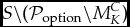 $S\backslash (\mathcal {P}_{\text{option}}\backslash M_{K}^{C})$ belongs to
 $\lbrace \mathcal {P}(x,K_{+}):x\in C(K_{+})\rbrace$, and so its intersection with
 $\mathcal {P}_{\text{option}}$ belongs to
 $\lbrace \mathcal {P} (x):x\in C(K_{+})\rbrace$. This intersection is precisely
 $S\cap \mathcal {P} _{\text{option}}\cap M_{K}^{C}$. Again by Claim 1, the bundle
 $S^{\prime }\backslash (\mathcal {P}_{\text{option}}\backslash M_{K}^{C})$ belongs to
 $\lbrace \mathcal {P}(x,K_{-}):x\in K_{-}\backslash C(K_{-})\rbrace$, and so its intersection with
 $\mathcal {P}_{\text{option}}$ belongs to
 $\lbrace \mathcal {P} (x):x\in K_{-}\backslash C(K_{-})\rbrace$, this intersection being
 $S^{\prime } \cap \mathcal {P}_{\text{option}}\cap M_{K}^{C}=S\cap \mathcal {P}_{\text{option} }\cap M_{K}^{C}$. Assuming Axiom 1*, the set
 $\lbrace \mathcal {P}(x):x\in K_{-}\backslash C(K_{-})\rbrace$ has no member in common with the set
 $\lbrace \mathcal {P}(x):x\in C(K_{-})\rbrace$, and so the latter set cannot also contain
 $S\cap \mathcal {P}_{\text{option}}\cap M_{K}^{C}$.
 $\blacksquare$
Lemma 5 Assume  $\mathcal {K}$ is diverse (and
 $\left|\mathcal {P} (x)\right|<\infty$ for all x ∈ X). Suppose Axioms 1*, 2**, and 3 hold. For all contexts
 $K,K^{\prime }\in \mathcal {K}$ and all options x, y ∈ K and x′, y′ ∈ K′, if we have xK = x′K′ and yK = y′K′ relative to the revealed reasons structure, then
 $$\begin{equation*}
\mathcal {P}(x,K)\succsim ^{C}\mathcal {\mathcal {P}}(y,K)\Leftrightarrow \mathcal {P}(x^{\prime },K^{\prime })\succsim ^{C}\mathcal {\mathcal {P}}(y^{\prime },K^{\prime }).
\end{equation*}$$
Proof. Let  $\mathcal {K}$ be diverse and
 $\left|\mathcal {P}(x)\right|<\infty$ for all x ∈ X. Consider
 $K,K^{\prime } \in \mathcal {K}$, x, y ∈ K and x′, y′ ∈ K′. For transparency, we will again add axioms only where they are needed. Consider the revealed reasons structure (M, ⩾) = (MC, ⩾C). (We do of course not assume that it explains the choice function C, although it does so under Axioms 1*, 2**, and 3 by Theorem 5, which will ultimately be proved.) Suppose xK = x′K′ and yK = y′K′. As
 $\mathcal {K}$ is diverse, it contains a context L in which only the bundles
 $\mathcal {P}(x,K)\backslash (\mathcal {P}_{\text{option}}\backslash M_{K})$ and
 $\mathcal {P}(y,K)\backslash (\mathcal {P}_{\text{option}}\backslash M_{K})$ are feasible, and a context L′ in which only the bundles
 $\mathcal {P}(x^{\prime },K^{\prime })\backslash (\mathcal {P}_{\text{option} }\backslash M_{K^{\prime }})$ and
 $\mathcal {P}(y^{\prime },K^{\prime } )\backslash (\mathcal {P}_{\text{option}}\backslash M_{K^{\prime }})$ are feasible. We now show three claims, where Claims 1 and 3 immediately imply the desired equivalence between
 $\mathcal {P}(x,K)\succsim ^{C}\mathcal {\mathcal {P} }(y,K)$ and
 $\mathcal {P}(x^{\prime },K^{\prime })\succsim ^{C} \mathcal {\mathcal {P}}(y^{\prime },K^{\prime })$.
Claim 1: Under Axiom 3,  $\mathcal {P}(x,K)\succsim ^{C}\mathcal {P}(y,K)$ if and only if
 $\mathcal {P}(x,K)\backslash (\mathcal {P}_{\text{option} }\backslash M_{K})$ is chosen in context L, and
 $\mathcal {P}(x^{\prime },K^{\prime })\succsim ^{C}\mathcal {P}(y^{\prime },K^{\prime })$ if and only if
 $\mathcal {P}(x^{\prime },K^{\prime })\backslash (\mathcal {P}_{\text{option} }\backslash M_{K^{\prime }})$ is chosen in context L′.
Suppose Axiom 3. We only show the first equivalence, as the second one holds analogously. There exist only finitely many option properties which are in  $\mathcal {P}(x,K)$ or
 $\mathcal {P}(y,K)$ but outside MK, because the set of these properties is
 $(\mathcal {P}(x)\cup \mathcal {P}(y))\backslash M_{K}$, where
 $\left|\mathcal {P}(x)\right|,\left|\mathcal {P} (y)\right|<\infty$. Let P 1, . . ., Pm (m ⩾ 0) be these properties. As
 $\mathcal {K}$ is diverse, it contains, for each t ∈ {0, 1, . . ., m}, a context Kt in which only the two bundles
 $\mathcal {P}(x,K)\backslash \lbrace P_{1},\ldots,P_{t}\rbrace$ and
 $\mathcal {P}(y,K)\backslash \lbrace P_{1},\ldots,P_{t}\rbrace$ are feasible. Since
 $$\begin{eqnarray*}
\begin{array}{l} \mathcal {P}(x,K)\backslash \lbrace P_{1},\ldots,P_{m}\rbrace =\mathcal {P}(x,K)\backslash (\mathcal {P}_{\text{option}}\backslash M_{K})\\
\mathcal {P}(y,K)\backslash \lbrace P_{1},\ldots,P_{m}\rbrace =\mathcal {P}(y,K)\backslash (\mathcal {P}_{\text{option}}\backslash M_{K}), \end{array} \ \ \ \ \
\end{eqnarray*}$$
we may assume that Km was chosen such that Km = L, and it suffices to show that  $\mathcal {P}(x,K)\succsim ^{C}\mathcal {P}(y,K)$ if and only if
 $\mathcal {P}(x,K)\backslash \lbrace P_{1},\ldots,P_{m}\rbrace$ is chosen in context Km. This is done by the following argument (which implicitly uses the fact that any context Kt has the same revealed motivationally salient properties as K, i.e. M(Kt) = MK):Footnote 35
$$\begin{eqnarray*}
\begin{array}{lll} & \mathcal {P}(x,K)\succsim ^{C}\mathcal {P}(y,K) & \\
\Leftrightarrow & \mathcal {P}(x,K)\text{ is chosen in }K_{0} & \text{ by Axiom 3}\\
\Leftrightarrow & \mathcal {P}(x,K)\backslash \lbrace P_{1}\rbrace \text{ is chosen in}\ K_{1} & \text{ as}\ P_{1} \text{ isn't revealed mot. sal. in}\ K_{1}\\
\Leftrightarrow & \mathcal {P}(x,K)\backslash \lbrace P_{1},P_{2}\rbrace \text{ is chosen in}\ K_{2} & \text{ as}\ P_{2} \text{ isn't revealed mot. sal. in}\ K_{2}\\
& \text{ etc}. & \\
\Leftrightarrow & \mathcal {P}(x,K)\backslash \lbrace P_{1},\ldots,P_{m}\rbrace \text{ is chosen in}\ K_{m} & \text{ as}\ P_{m} \text{ isn't revealed mot. sal. in}\ K_{m}. \end{array} \ \ \ \ \ \
\end{eqnarray*}$$
Claim 2: Under Axioms 2**,  $\lbrace \mathcal {P}(z):z\in C(L)\rbrace =\lbrace \mathcal {P} (z):z\in C(L^{\prime })\rbrace$.
Assume Axiom 2**. It suffices to show that both premises of the axiom (applied to the contexts L and L′) hold. Note first that the set  $\lbrace \mathcal {P}(z,L):z\in L\rbrace$ consists of the bundles
 $\mathcal {P} (x,K)\backslash (\mathcal {P}_{\text{option}}\backslash M_{K})$ and
 $\mathcal {P}(y,K)\backslash (\mathcal {P}_{\text{option}}\backslash M_{K})\rbrace$. When intersected with
 $\mathcal {P}_{\text{option}}$, these two bundles become
 $$\begin{eqnarray*}
\mathcal {P}(x,K)\cap M_{K}\cap \mathcal {P}_{\text{option}} & =&\mathcal {P} (x,K)\cap M_{K}=x_{K}\\
\text{and }\mathcal {P}(y,K)\cap M_{K}\cap \mathcal {P}_{\text{option}} & =&\mathcal {P}(y,K)\cap M_{K}=y_{K}\text{,}
\end{eqnarray*}$$
where the middle equality on both lines holds because  $M_{K}\subseteq \mathcal {P}_{\text{option}}$ by Lemma 4. Since
 $\lbrace \mathcal {P}(z):x\in L\rbrace$ consists precisely of the intersections of a bundle in
 $\lbrace \mathcal {P} (z,L):z\in L\rbrace$ with
 $\mathcal {P}_{\text{option}}$, we have
 $\lbrace \mathcal {P} (z):z\in L\rbrace =\lbrace x_{K},y_{K}\rbrace$. By an analogous argument,
 $\lbrace \mathcal {P} (z):z\in L^{\prime }\rbrace =\lbrace x_{K^{\prime }}^{\prime },y_{K^{\prime }}^{\prime }\rbrace$. Since, by assumption xK = x′K′ and yK = y′K′, it follows that
 $\lbrace \mathcal {P}(z):z\in L\rbrace =\lbrace \mathcal {P}(z):z\in L^{\prime }\rbrace$. This identity is the first premise of Axiom 2** applied to the contexts L and L′. The axiom’s second premise also holds, since
• for each z in L, any property in
$\mathcal {P}(z)$ belongs to xK or yK, so to MK = ML; and• for each z in L′, any property in
$\mathcal {P}(z)$ belongs to x′K′ or y′K′, so to M K′ = M L′.


Claim 3: Under Axioms 1* and 2**,  $\mathcal {P}(x,K)\backslash (\mathcal {P}_{\text{option}}\backslash M_{K})$ is chosen in context L if and only if
 $\mathcal {P}(x^{\prime },K^{\prime })\backslash (\mathcal {P} _{\text{option}}\backslash M_{K^{\prime }})$ is chosen in context L′.
Suppose Axioms 1* and 2** hold. We assume that  $\mathcal {P}(x,K)\backslash (\mathcal {P}_{\text{option}}\backslash M_{K})$ is chosen in context L and show that
 $\mathcal {P}(x^{\prime },K^{\prime })\backslash (\mathcal {P} _{\text{option}}\backslash M_{K^{\prime }})$ is chosen in context L′ (the converse implication has an analogous proof). Since the bundle
 $\mathcal {P}(x^{\prime },K^{\prime })\backslash (\mathcal {P}_{\text{option} }\backslash M_{K^{\prime }})$ belongs to
 $\lbrace \mathcal {P}(z,L^{\prime }):z\in L^{\prime }\rbrace$, we can pick a z′ ∈ L′ such that
 $\mathcal {P}(z^{\prime },L^{\prime })=\mathcal {P}(x^{\prime },K^{\prime })\backslash (\mathcal {P}_{\text{option}}\backslash M_{K^{\prime }})$. Note that
 $$\begin{eqnarray*}
\mathcal {P}(z^{\prime }) & =&\mathcal {P}(z^{\prime },L^{\prime })\cap \mathcal {P}_{\text{option}}=\mathcal {P}(x^{\prime },K^{\prime })\cap \mathcal {P}_{\text{option}}\cap M_{K^{\prime }}\\
& =&\mathcal {P}(x^{\prime },K^{\prime })\cap M_{K^{\prime }}=x_{K^{\prime } }^{\prime }=x_{K},
\end{eqnarray*}$$
where the third equality holds because  $M_{K^{\prime }}\subseteq \mathcal {P} _{\text{option}}$ by Lemma 4. Meanwhile, since the bundle
 $\mathcal {P}(x,K)\backslash (\mathcal {P}_{\text{option}}\backslash M_{K})$ belongs to
 $\lbrace \mathcal {P}(z,L):z\in C(L)\rbrace$, its intersection with
 $\mathcal {P}_{\text{option}}$ belongs to
 $\lbrace \mathcal {P}(z):z\in C(L)\rbrace$. By the proof of Claim 2, that intersection is xK, so that
 $x_{K} \in \lbrace \mathcal {P}(z):z\in C(L)\rbrace$. By Claim 2 and the fact that
 $x_{K} =\mathcal {P}(z^{\prime })$, it follows that
 $\mathcal {P}(z^{\prime } )\in \lbrace \mathcal {P}(z):z\in C(L^{\prime })\rbrace$. So z ∈ C(L′) for some, and hence by Axiom 1* every z ∈ L′ such that
 $\mathcal {P}(z)=\mathcal {P}(z^{\prime })$. In particular, z′ ∈ C(L′). Hence the bundle
 $\mathcal {P}(z^{\prime },L^{\prime })=\mathcal {P}(x^{\prime },K^{\prime })\backslash (\mathcal {P}_{\text{option} }\backslash M_{K^{\prime }})$ is chosen in context L′, as desired.
 $\blacksquare$
Proof of Theorem 5. Assume  $\mathcal {K}$ is diverse and
 $\left|\mathcal {P}(x)\right|<\infty$ for all x ∈ X. We prove first the axioms’ necessity (Step 1) and then their sufficiency (Step 2).
Step 1. Suppose C has a reason-based explanation with context-unrelated motivation (M, ⩾). Axiom 3 holds by Theorem 1. To see why Axioms 1* holds, note that, for all  $K\in \mathcal {K}$ and x, y ∈ K,
 $\mathcal {P}(x)=\mathcal {P}(y)\Rightarrow x_{K}=y_{K}$ because
 $M_{K} \subseteq \mathcal {P}_{\text{option}}$.
To show that Axiom 2** holds, we consider contexts  $K,K^{\prime }\in \mathcal {K}$ such that (*)
 $\lbrace \mathcal {P}(x):x\in K\rbrace =\lbrace \mathcal {P}(x):x\in K^{\prime }\rbrace$ and (**)
 $\mathcal {P}(x)\subseteq M_{K}^{C},M_{K^{\prime }}^{C}$ for all x in K or K′. We first show that
 $$\begin{equation}
x_{K}=\mathcal {P}(x)\text{ for all }x\in K \text{ and } x_{K^{\prime } }=\mathcal {P}(x) \text{\ for all }x\in K^{\prime }\text{.}
\end{equation}$$
The first part of (4) holds since, for any x ∈ K,
 $$\begin{eqnarray*}
\begin{array}{lll@{\quad}l} x_{K} & = & \mathcal {P}(x,K)\cap M_{K} & \text{by definition of }x_{K} \\
& = & \mathcal {P}(x,K)\cap \mathcal {P}_{\text{option}}\cap M_{K} & \text{as }M_{K}\subseteq \mathcal {P}_{\text{option}}\\
& = & \mathcal {P}(x)\cap M_{K} & \text{as }\mathcal {P}(x)=\mathcal {P} (x,K)\cap \mathcal {P}_{\text{option}}\\
& = & \mathcal {P}(x) & \text{as }\mathcal {P}(x)\subseteq M_{K} ^{C}\subseteq M_{K}, \end{array} \ \ \
\end{eqnarray*}$$
where the last-mentioned inclusion ‘MCK⊆MK’ holds by Lemma 3. The second part of (4) holds for analogous reasons.
It is now easy to see why  $\lbrace \mathcal {P}(y):y\in C(K)\rbrace =\lbrace \mathcal {P} (y^{\prime }):y^{\prime }\in C(K^{\prime })\rbrace$. Let us show why the left side is included in the right side (the converse inclusion is analogous). We thus consider a y ∈ C(K) and show that
 $\mathcal {P}(y)\in \lbrace \mathcal {P} (y^{\prime }):y^{\prime }\in C(K^{\prime })\rbrace$. By (*), we can pick a y′ ∈ K′ such that
 $\mathcal {P}(y)=\mathcal {P}(y^{\prime })$. It suffices to show that y′ ∈ C(K′). This follows from the fact that y ∈ C(K) and the following equivalences:
 $$\begin{eqnarray*}
\begin{array}{lll@{\quad}l} y\in C(K) & \Leftrightarrow & y_{K}\ge x_{K} \text{ for all}\ x\in K & \text{ as}\ (M,\ge ) \text{ explains}\ C\\
& \Leftrightarrow & \mathcal {P}(y)\ge \mathcal {P}(x) \text{ for all}\ x\in K & \text{ by}\ (4)\\
& \Leftrightarrow & \mathcal {P}(y^{\prime })\ge \mathcal {P}(x) \text{ for all}\ x\in K^{\prime } & \text{ by}\ \mathcal {P}(y)=\mathcal {P}(y^{\prime }) \text{ and}\ (^{*})\\
& \Leftrightarrow & y_{K^{\prime }}^{\prime }\ge x_{K^{\prime }} \text{ for all}\ x\in K^{\prime } & \text{ by}\ (4)\\
& \Leftrightarrow & y^{\prime }\in C(K^{\prime }) & \text{ as}\ (M,\ge ) \text{ explains}\ C. \end{array} \
\end{eqnarray*}$$
Step 2. Conversely, assume Axioms 1*, 2**, and 3. Let (M, ⩾) be the revealed reasons structure (MC, ⩾C) defined in Appendix A. Since this reasons structure has context-unrelated motivation by Lemma 4, it suffices to show that it explains C. We thus consider any  $K\in \mathcal {K}$ and x ∈ K and have to show that
 $$\begin{equation*}
x\in C(K)\Leftrightarrow \left[ x_{K}\ge y_{K}\text{ for all }y\in K\right] \text{.}
\end{equation*}$$
First, if x ∈ C(K), then, for all y ∈ K, we have xK ⩾ yK, by definition of ⩾ as ⩾ C and by the fact that some option perceived as xK (namely x itself) is chosen in K while some option perceived as yK (namely y itself) is feasible in K.
Conversely, assume that xK ⩾ yK for all y ∈ K. Consider any y ∈ K. By definition of ⩾ , since xK ⩾ yK, there is a context  $K^{\prime }\in \mathcal {K}$ in which some chosen option x′ ∈ C(K′) is perceived as x′K′ = xK and some feasible option y′ ∈ K′ is perceived as y′K′ = yK. Since x′ ∈ C(K′) and y′ ∈ K′, we have
 $\mathcal {P}(x^{\prime },K^{\prime })\succsim ^{C}\mathcal {\mathcal {P}}(y^{\prime },K^{\prime })$. Since x′K′ = xK and y′K′ = yK, it follows that
 $\mathcal {P}(x,K)\succsim ^{C}\mathcal {\mathcal {P}}(y,K)$ by Lemma 5. As this is true for all y ∈ K, we have x ∈ C(K), by Axiom 3
 $^{\text{+}}$ (which holds by Lemma 2).
 $\blacksquare$
B.2. The results on reason-based prediction
We now adopt our extended framework for predictions defined in Section 7. As mentioned in Section 7.2, we further assume that each context  $K\in \mathcal {K}$ has only finitely many context properties, i.e.
 $\left|\mathcal {P}(K)\right|<\infty$.
Proof of Proposition 2. Let  $\mathcal {R}^{\prime }=(M^{\prime },\ge )$ be a reasons structure for a domain
 $\mathcal {D} \subseteq \mathcal {K}$. Regarding part (a), if all M′K coincide, then obviously
 $C\!AU^{\mathcal {R}^{\prime }}=\varnothing$; and if
 $C\!AU^{\mathcal {R}^{\prime }}=\varnothing$, then part (b) will imply that all M′K coincide. It thus remains to prove part (b). We proceed by contraposition. Let
 $K,K^{\prime }\in \mathcal {D}$ satisfy M′K ≠ M K′′. Since
 $\mathcal {P}(K)$ and
 $\mathcal {P}(K^{\prime })$ are finite, the ‘disagreement set’
 $\mathcal {P}(K)\bigtriangleup \mathcal {P}(K^{\prime })$ is finite (for any two sets A and B, we define A△B as (A\B)∪(B\A)). So, as one easily checks, there is a finite sequence
 $K_{1},\ldots,K_{n}\in \mathcal {D}$ with K 1 = K, Kn = K′ such that, for each m ∈ {1, . . ., n − 1}, the contexts Km and K m + 1 differ minimally (in the sense of (cau3)). Since M′K 1 ≠ M′Kn, there is an m ∈ {1, . . ., n − 1} such that M′Km ≠ M′K m + 1. By definition of reasons structures, it follows that
 $\mathcal {P}(K_{m} )\ne \mathcal {P}(K_{m+1})$. Hence we may pick a context property
 $P\in \mathcal {P}(K_{m})\bigtriangleup \mathcal {P}(K_{m+1})$. It follows that
 $P\in \mathcal {P}(K)\bigtriangleup \mathcal {P}(K^{\prime })$. Hence, since we also have
 $P\in C\!AU^{\mathcal {R}^{\prime }}$ (because the criteria (cau1)-(cau3) hold for the contexts Km and K m + 1),
 $P\in (\mathcal {P}(K)\cap C\!AU^{\mathcal {R}^{\prime }})\bigtriangleup (\mathcal {P} (K^{\prime })\cap C\!AU^{\mathcal {R}^{\prime }})$. So
 $\mathcal {P}(K)\cap C\!AU^{\mathcal {R}^{\prime }}\ne \mathcal {P}(K^{\prime })\cap C\!AU^{\mathcal {R} ^{\prime }}$.
 $\blacksquare$
Proof of Remark 1. Consider an explanation  $\mathcal {R}=(M,\ge )$ of the observed choice function
 $C_{\text{o}}$. Let
 $\mathcal {R}^{1}=(M^{1},\ge )$,
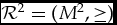 $\mathcal {R}^{2}=(M^{2},\ge )$, and
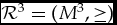 $\mathcal {R}^{3}=(M^{3},\ge )$ be the reasons structures used to define, respectively, the cautious, semi-courageous and courageous predictors, with corresponding domains
 $\mathcal {D}^{1}$,
 $\mathcal {D}^{2}$ and
 $\mathcal {D} ^{3}$.
(a)
$C^{\mathcal {R}^{1}}$ extends $C_{\text{o}}$, because $\mathcal {R}^{1}$ extends $\mathcal {R}$ (as a consequence of the definition of $\mathcal {R}^{1}$) and $C^{\mathcal {R}}=C_{\text{o}}$ (by assumption).(b) We prove that
$C^{\mathcal {R}^{2}}$ extends $C^{\mathcal {R}^{1}}$ by showing that $\mathcal {R}^{2}$ extends $\mathcal {R}^{1}$. Consider any $K\in \mathcal {D}^{1}$. We have to show that $K\in \mathcal {D}^{2}$ and M 1K = MK 2. Since $K\in \mathcal {D}^{1}$, there is an $L\in \mathcal {K}_{\text{o}}$ such that {P(x, K): x ∈ K} = {P(x, L): x ∈ L}. One easily verifies the conditions (i) (by using the same context L) and (ii) (by using the context L′ ≔ L ).(c) It suffices to show that
$\mathcal {R}^{3}$ extends $\mathcal {R}^{2}$. Let $K\in \mathcal {D}^{2}$; so conditions (i) and (ii) hold. We have to show that $K\in \mathcal {D}^{3}$ and M 2K = MK 3. The former holds because (i) immediately implies (i*) (just use the same context $L\in \mathcal {K} _{\text{o}}$). Moreover, M 2K = MK 3 because each side equals ML for L as in (i). $\blacksquare$


Proof of Theorem 2. Consider an explanation  $\mathcal {R}=(M,\ge )$ of the observed choice function
 $C_{\text{o}}$. We use the notation from our proof of Remark 1. Further, for any reasons structure
 $\mathcal {R}^{\prime }$, the set of feasible options as perceived in a context K (from the domain of
 $\mathcal {R}^{\prime }$) is denoted
 $K^{\mathcal {R}^{\prime }}:=\lbrace x_{K}^{\mathcal {R}^{\prime }}:x\in K\rbrace$.
(a) Suppose C is explicable by an arbitrary reasons structure
$\mathcal {R} ^{+}=(M^{+},\ge ^{+})$. Consider any $K\in \mathcal {D}^{1}$ and x ∈ K. We have to show that $x\in C^{\mathcal {R}^{1}}(K)\Leftrightarrow x\in C(K)$. As $K\in \mathcal {D}^{1}$ we can pick an $L\in \mathcal {K}_{\text{o}}$ such that
(5)So
$$\begin{equation}
\lbrace \mathcal {P}(y,K):y\in K\rbrace =\lbrace \mathcal {P}(y,L):y\in L\rbrace .
\end{equation}$$
$K^{\mathcal {R}^{1}}=L^{\mathcal {R}^{1}}$ and $K^{\mathcal {R}^{+} }=L^{\mathcal {R}^{+}}$ (though perhaps $K^{\mathcal {R}^{1}}\ne K^{\mathcal {R} ^{+}}$). Now pick a z ∈ L such that $\mathcal {P}(x,K)=\mathcal {P}(z,L)$ (which is possible by (5)). It follows that $x_{K}^{\mathcal {R}^{1} }=z_{L}^{\mathcal {R}^{1}}$ and $x_{K}^{\mathcal {R}^{+}}=z_{L}^{\mathcal {R} ^{+}}$. We show the claimed equivalence by proving that each side holds if and only if $z\in C_{\text{o}}(L)$:
$$\begin{eqnarray*}
\begin{array}{ll@{\quad}l} x\in C^{\mathcal {R}^{1}}(K) & \Leftrightarrow x_{K}^{\mathcal {R}^{1}}\ge S\text{ for all }S\in K^{\mathcal {R}^{1}} & \text{by definition of } C^{\mathcal {R}^{1}}\\
& \Leftrightarrow z_{L}^{\mathcal {R}^{1}}\ge S\text{ for all }S\in L^{\mathcal {R}^{1}} & \text{as }x_{K}^{\mathcal {R}^{1}}=z_{L}^{\mathcal {R} ^{1}}\text{ and } K^{\mathcal {R}^{1}}=L^{\mathcal {R}^{1}}\\
& \Leftrightarrow z\in C^{\mathcal {R}^{1}}(L) & \text{ by definition of}\ C^{\mathcal {R}^{1}}\\
& \Leftrightarrow z\in C_{\text{o}}(L) & \text{ as}\ C^{\mathcal {R}^{1} }(L)=C_{\text{o}}(L) \text{ by Remark 1},\\
x\in C(K) & \Leftrightarrow x\in C^{\mathcal {R}^{+}}(K) & \text{ as}\ C^{\mathcal {R}^{+}}=C\\
& \Leftrightarrow x_{K}^{\mathcal {R}^{+}}\ge ^{+}S\text{ for all }S\in K^{\mathcal {R}^{+}} & \text{by definition of }C^{\mathcal {R}^{+}}\\
& \Leftrightarrow z_{L}^{\mathcal {R}^{+}}\ge ^{+}S\text{ for all }S\in L^{\mathcal {R}^{+}} & \text{as }x_{K}^{\mathcal {R}^{+}}=z_{L}^{\mathcal {R} ^{+}}\text{ and }K^{\mathcal {R}^{+}}=L^{\mathcal {R}^{+}}\\
& \Leftrightarrow z\in C^{\mathcal {R}^{+}}(L) & \text{ by definition of}\ C^{\mathcal {R}^{+}}\\
& \Leftrightarrow z\in C_{\text{o}}(L) & \text{ as}\ C^{\mathcal {R}^{+} }(L)=C(L)=C_{\text{o}}(L). \end{array}
\end{eqnarray*}$$
(b) Now let C be explicable by an extension
$\mathcal {R}^{+}=(M^{+},\ge )$ of $\mathcal {R}$. Let $K\in \mathcal {D}^{2}$ and x ∈ K. We show that $x\in C^{\mathcal {R}^{2}}(K)\Leftrightarrow x\in C(K)$. As $K\in \mathcal {D}^{2}$ we can pick $L,L^{\prime }\in \mathcal {K}_{\text{o}}$ such that $\mathcal {P} (L)=\mathcal {P}(K)$ and (*) $K^{\mathcal {R}^{2}}=(L^{\prime })^{\mathcal {R} ^{2}}$. By (*), we can choose a z ∈ L′ such that (**) $x_{K}^{\mathcal {R}^{2}}=z_{L^{\prime }}^{\mathcal {R}^{2}}$. Since M +L′ = M L′2 (= M L′),
(6)Since M +L = ML 2 (= ML) and
$$\begin{equation}
(L^{\prime })^{\mathcal {R}^{+}}=(L^{\prime })^{\mathcal {R}^{2}}\quad \text{ and }\quad z_{L^{\prime }}^{\mathcal {R}^{+}}=z_{L^{\prime }}^{\mathcal {R}^{2}}.
\end{equation}$$
$\mathcal {P}(L)=\mathcal {P}(K)$, we have M +K = MK 2, and thus
(7)By (*), (**), (6), and (7), we have (***)
$$\begin{equation}
K^{\mathcal {R}^{+}}=K^{\mathcal {R}^{2}}\quad\text{ and }\quad x_{K}^{\mathcal {R}^{+} }=x_{K}^{\mathcal {R}^{2}}.
\end{equation}$$
$K^{\mathcal {R}^{+} }=(L^{\prime })^{\mathcal {R}^{+}}$ and (****) $x_{K}^{\mathcal {R}^{+} }=z_{L^{\prime }}^{\mathcal {R}^{+}}$.One can prove the claimed equivalence by proving that each side holds if and only if
$z\in C_{\text{o}}(L)$. One should follow the steps taken similarly in the proof of part (a): it suffices to replace L by L′ and $\mathcal {R}^{1}$ by $\mathcal {R}^{2}$, and to apply the identities (*)-(****).(c) Finally, let C be explicable by an extension
$\mathcal {R}^{+} =(M^{+},\ge )$ of $\mathcal {R}$ with $C\!AU^{\mathcal {R}^{+}}=C\!AU^{\mathcal {R}}$. Let $K\in \mathcal {D}^{3}$ and x ∈ K. We prove $x\in C^{\mathcal {R}^{3} }(K)\Leftrightarrow x\in C(K)$. Since $K\in \mathcal {D}^{3}$, we can pick $L,L^{\prime }\in \mathcal {K}_{\text{o}}$ such that $\mathcal {P}(L)\cap C\!AU^{\mathcal {R}}=\mathcal {P}(K)\cap C\!AU^{\mathcal {R}}$, M 3K = ML 3, and ($^{\text{+}}$) $K^{\mathcal {R}^{3}}=(L^{\prime })^{\mathcal {R}^{3}}$. Since $C\!AU^{\mathcal {R}^{+}}=C\!AU^{\mathcal {R}}$ and $\mathcal {P}(L)\cap C\!AU^{\mathcal {R}}=\mathcal {P}(K)\cap C\!AU^{\mathcal {R}}$, we have $\mathcal {P}(L)\cap C\!AU^{\mathcal {R}^{+}}=\mathcal {P}(K)\cap C\!AU^{\mathcal {R} ^{+}}$, and thus, by Proposition 2, M +L = MK +. By ($^{\text{+}}$), there is a z ∈ L′ such that ($^{\text{++}}$) $x_{K}^{\mathcal {R}^{3}}=z_{L^{\prime }}^{\mathcal {R}^{3}}$. Since M +L′ = M L′3 (= M L′), we have
(8)Since M +L = ML 3 (= ML), M +L = MK +, and M 3L = MK 3, we have M +K = MK 3, and thus
$$\begin{equation}
(L^{\prime })^{\mathcal {R}^{+}}=(L^{\prime })^{\mathcal {R}^{3}}\quad \text{ and }\quad z_{L^{\prime }}^{\mathcal {R}^{+}}=z_{L^{\prime }}^{\mathcal {R}^{3}}.
\end{equation}$$
(9)By (
$$\begin{equation}
K^{\mathcal {R}^{+}}=K^{\mathcal {R}^{3}}\quad\text{ and }\quad x_{K}^{\mathcal {R}^{+} }=x_{K}^{\mathcal {R}^{3}}.
\end{equation}$$
$^{\text{+}}$), ($^{\text{++}}$), (8), and (9), we have ($^{\text{+++}}$) $K^{\mathcal {R}^{+}}=(L^{\prime })^{\mathcal {R}^{+}}$ and ($^{\text{++++}}$) $x_{K}^{\mathcal {R}^{+}}=z_{L^{\prime }}^{\mathcal {R}^{+}}$. The claimed equivalence can once again be proved by establishing that each side holds if and only if $z\in C_{\text{o}}(L)$; one should use the same argument as for part (a), replacing L by L′ and $\mathcal {R}^{1}$ by $\mathcal {R}^{3}$, and drawing on the identities ($^{\text{+}}$)-($^{\text{++++}}$). $\blacksquare$